Untrained CNNs Match Backpropagation at V1: A Systematic RSA Comparison of Four Learning Rules Against Human fMRI

Abstract

A central question in computational neuroscience is whether the learning rule used to train a neural network determines how well its internal representations align with those of the human visual cortex. We present a systematic comparison of four learning rules—backpropagation (BP), feedback alignment (FA), predictive coding (PC), and spike-timing-dependent plasticity (STDP)—applied to identical convolutional architectures and evaluated against human fMRI data from the THINGS-fMRI dataset (720 stimuli, 3 subjects) using Representational Similarity Analysis (RSA). All models process stimuli at $224\times 224$ resolution; results are averaged across 5 random seeds. Crucially, we include an untrained random-weights baseline that reveals the dominant role of architecture. At V1/V2, the untrained baseline exceeds backpropagation ($\rho=0.076$ vs. $\rho=0.034$; $\Delta\rho=+0.044$, $p<0.001$), and STDP achieves the highest V1 alignment among trained rules ($\rho=0.064$). At LOC, only BP reliably exceeds the random baseline ($\rho=0.012$ vs. $-0.005$, $p<0.001$). At IT, all five conditions converge ($\rho=0.008$–$0.014$) with no significant pairwise differences among trained rules ($p>0.05$, FDR-corrected). FA consistently produces the lowest alignment at V1, V2, and LOC ($\rho=0.012$ at V1, below all other conditions). Partial RSA confirms all effects survive pixel-similarity control. Seed variability is small relative to between-rule differences at V1/V2. These results demonstrate that early visual alignment is architecture-driven, learning rules differentiate only at intermediate areas, and all rules converge at the highest levels of the hierarchy.

Keywords: representational similarity analysis, visual cortex, biologically plausible learning, random baseline, STDP, feedback alignment, predictive coding, fMRI, THINGS

1 Introduction

Deep neural networks (DNNs) trained with backpropagation have become the dominant computational models of the ventral visual stream (Yamins and DiCarlo,, 2016). A well-established finding is that the hierarchy of features learned by DNNs mirrors the hierarchy of representations from V1 through IT cortex, as quantified by representational similarity analysis (RSA) and related metrics (Kriegeskorte et al.,, 2008; Schrimpf et al.,, 2020). This correspondence has been interpreted as evidence that the objectives and inductive biases of deep learning capture something fundamental about visual processing.

Yet backpropagation is neurobiologically implausible in at least three well-known respects: it requires symmetric forward and feedback weights (the weight transport problem), it relies on a global error signal propagated backward through the network, and the forward and backward passes must be temporally separated (Crick,, 1989; Lillicrap et al.,, 2020). These observations have motivated work on biologically plausible alternatives, including feedback alignment (Lillicrap et al.,, 2016), predictive coding (Rao and Ballard,, 1999; Whittington and Bogacz,, 2017), and spike-timing-dependent plasticity (Bi and Poo,, 1998).

A key question is: does the choice of learning rule matter for brain alignment? If alignment arises from the architecture and objective rather than the weight-update rule, then alternative rules—or even no training at all—should yield comparable alignment. Prior work has compared individual learning rules to brain data (Schrimpf et al.,, 2020), but to our knowledge no study has systematically compared all four rules together with an untrained random-weights baseline on the same architecture, stimuli, and RSA pipeline.

We address this gap with five conditions: BP, FA, PC, STDP, and a random-weights (untrained) baseline, all applied to identical CNNs trained on CIFAR-10, with layer-wise RDMs compared to human fMRI from the THINGS-fMRI dataset.

Our main contributions are: (1) a head-to-head RSA comparison of four learning rules plus a random baseline at $224\times 224$ resolution, averaged across 5 seeds; (2) the finding that V1/V2 alignment is architecture-driven, with the untrained CNN exceeding BP at V1 ($\Delta\rho=+0.044$, $p<0.001$); (3) the result that at IT, all trained rules converge and are statistically indistinguishable from each other; (4) the finding that only LOC shows a reliable learning effect, with BP being the sole rule to significantly exceed the random baseline; and (5) the consistent finding that FA produces the lowest brain alignment at V1, V2, and LOC.

2 Related Work

RSA as a model evaluation tool. Kriegeskorte et al., (2008) introduced RSA as a framework for comparing representations across measurement modalities. The core idea is to represent each system’s response to a stimulus set as a pairwise dissimilarity matrix (RDM) and to assess model–brain alignment as the rank correlation between RDMs. RSA has since become a standard tool for comparing DNNs to neural data (Yamins and DiCarlo,, 2016; Schrimpf et al.,, 2020).

DNNs and the visual hierarchy. Task-optimized DNNs reproduce the representational hierarchy of the ventral visual stream, with early layers matching V1 and deeper layers matching IT (Yamins and DiCarlo,, 2016). The Brain-Score benchmark (Schrimpf et al.,, 2020) systematizes this evaluation across architectures and datasets. Most high-scoring models are trained with standard BP on ImageNet. Importantly, Schrimpf et al., (2020) noted that untrained networks retain some brain alignment, but did not systematically compare this against multiple learning rules.

Biologically plausible learning rules. Feedback alignment (Lillicrap et al.,, 2016) replaces the transpose weight matrix in the backward pass with fixed random matrices, removing the weight transport problem. Lillicrap et al., (2016) showed that FA still allows learning in fully-connected networks, though its effectiveness in convolutional architectures is less established. Predictive coding (Rao and Ballard,, 1999) frames inference as hierarchical prediction-error minimization; Whittington and Bogacz, (2017) showed that PC implements an approximation to BP under certain conditions, with learning driven entirely by local Hebbian updates. Spike-timing-dependent plasticity (Bi and Poo,, 1998) updates synaptic weights based on the relative timing of pre- and postsynaptic spikes, and is one of the best-characterized forms of synaptic plasticity in mammalian cortex. Each of these rules has been studied individually in the context of neural representation learning, but direct comparisons on identical architectures and evaluation pipelines are rare.

Random networks and early visual cortex. Saxe et al., (2011) demonstrated that random-weight networks can exhibit non-trivial visual structure. Concurrently with our work, Truzzi and Cusack, (2025) showed that random-weight CNNs predict early visual cortex responses when model complexity is sufficient. Our work extends these observations by systematically comparing four distinct learning rules against the random baseline, and by demonstrating that the architecture-dominance effect is not limited to V1: at IT, all rules—including random—converge with no significant pairwise differences.

Sparse coding and V1. Olshausen and Field, (1996) showed that unsupervised learning of a sparse code for natural images produces receptive fields resembling V1 simple cells, establishing that correlation-based learning from image statistics suffices to produce V1-like representations without supervised objectives.

3 Methods

3.1 Dataset

We used the THINGS-fMRI dataset (Gifford and Cichy,, 2022), comprising 7T fMRI responses to images from the THINGS object concept database (Hebart et al.,, 2019). We selected 720 stimuli (one image per concept). fMRI responses were available for 3 subjects across 4 regions of interest (ROIs): V1, V2, LOC, and IT. RDMs were computed from averaged trial responses using correlation distance, then averaged across subjects to produce a single mean-brain RDM per ROI.

3.2 Model Architecture

All five conditions used an identical CNN architecture consisting of three convolutional layers (Conv1–Conv3, each followed by BatchNorm, ReLU, and $2\times 2$ max-pooling) and two fully connected layers (FC1, FC2). The output layer uses softmax for 10-class classification on CIFAR-10. Training used 8,000 CIFAR-10 samples for 40 epochs at native $32\times 32$ resolution. For RSA evaluation, THINGS stimuli were resized to $224\times 224$ and passed through the same trained (or untrained) network; this is standard practice in model–brain comparisons where training and evaluation datasets differ (Schrimpf et al.,, 2020).

The layer-to-ROI mapping follows the standard ventral stream correspondence: Conv1$\to$V1, Conv1$\to$V2, Conv3$\to$LOC, FC1$\to$IT.

Figure 1: Model architecture and layer-to-ROI mapping. Models are trained on CIFAR-10 ($32\times 32$); for RSA, THINGS stimuli are resized to $224\times 224$ at feature extraction time. Dashed arrows: Conv1$\to$V1, Conv1$\to$V2, Conv3$\to$LOC, FC1$\to$IT.

3.3 Learning Rules

Random Weights serves as the architectural baseline. The network is initialized with He-normal weights and never trained, isolating the contribution of the convolutional architecture (filters, ReLU, pooling) to brain alignment.

Backpropagation (BP) serves as the supervised baseline: $\Delta W_{l}=-\eta\frac{\partial\mathcal{L}}{\partial W_{l}}$.

Feedback Alignment (FA) (Lillicrap et al.,, 2016) replaces $\mathbf{W}_{l}^{\top}$ in the backward pass with a fixed random matrix $\mathbf{B}_{l}$:

$$\Delta W_{l}=\delta_{l}^{\text{FA}}\mathbf{h}_{l-1}^{\top},\quad\delta_{l}^{\text{FA}}=f^{\prime}(z_{l})\odot(\mathbf{B}_{l+1}\delta_{l+1}^{\text{FA}}).$$ (1)

Predictive Coding (PC) (Rao and Ballard,, 1999; Whittington and Bogacz,, 2017) minimizes a hierarchical prediction-error energy $F=\sum_{l}\|\varepsilon_{l}\|^{2}$ through iterative inference ($T_{\text{inf}}=10$ steps, inference rate $\alpha=0.02$):

$$\Delta W_{l}\propto\varepsilon_{l}\mathbf{x}_{l-1}^{\top}.$$ (2)

Prediction weights $\mathbf{P}_{l}$ (implemented as transposed convolutions) generate top-down predictions; prediction errors $\varepsilon_{l}=r_{l}-\hat{r}_{l}$ drive both inference dynamics (updating representations $r_{l}$) and weight learning (weight rate $\eta_{W}=10^{-4}$). As with STDP, only convolutional weights are updated via PC; the fully connected readout layers are trained with backpropagation.

STDP (Bi and Poo,, 1998) converts activations to Poisson spike trains ($T=10$ timesteps) and uses first-spike timing to update convolutional weights:

$$\Delta w=\begin{cases}A_{+}e^{-\Delta t/\tau_{+}}&\Delta t>0\text{ (LTP)}\\ -A_{-}e^{\Delta t/\tau_{-}}&\Delta t<0\text{ (LTD)}\end{cases}$$ (3)

with $\tau_{+}=\tau_{-}=20$ ms, $A_{+}=A_{-}=0.003$, $\text{lr}=5\times 10^{-4}$. Only the convolutional layers (Conv1–Conv3) are updated via STDP; the fully connected layers (FC1, FC2) are trained with backpropagation to provide a supervised readout, analogous to a linear probe on STDP-learned features. The 63% CIFAR-10 accuracy therefore reflects STDP feature quality evaluated through a BP-trained classifier, not end-to-end STDP learning.

3.4 RSA Pipeline

Feature extraction. For each layer, activations were extracted on the 720 THINGS stimuli (resized to $224\times 224$, standard ResNet input resolution). Convolutional activations were spatially averaged (global average pooling). All results are averaged across 5 random seeds per learning rule; error bars in figures reflect seed variability (mean $\pm$ std).

RDM construction. Model RDMs were computed as $1-r$ (correlation distance). Brain RDMs were averaged across subjects to produce a single mean-brain RDM per ROI.

RSA score. Model–brain alignment was quantified as Spearman’s $\rho$ between the upper triangles of model and mean-brain RDMs.

Bootstrap confidence intervals. 95% CIs were estimated by bootstrap resampling ($N=10{,}000$) of the stimulus pairs from the mean-brain RDM comparison. This sample size is sufficient for stable CI estimation at the correlation values observed here.

Noise ceiling. Upper and lower bounds were estimated using split-half reliability corrected by the Spearman–Brown formula (Kriegeskorte et al.,, 2008).

3.5 Statistical Tests

Pairwise differences between conditions were assessed using permutation tests ($N=1{,}000$). For each pair of conditions $A$ and $B$, we computed the observed difference $\Delta\rho=\rho(A,\text{brain})-\rho(B,\text{brain})$. Under $H_{0}\colon\Delta\rho=0$, the brain RDM vector was randomly permuted to generate a null distribution of $\Delta\rho$ values; $p$ is the fraction of null $|\Delta\rho|$ values exceeding the observed $|\Delta\rho|$. Because the minimum resolvable $p$-value at $N=1{,}000$ is $p=0.001$, all $p$-values reported as $p<0.001$ should be interpreted as $p\leq 0.001$. All 40 pairwise comparisons (10 pairs $\times$ 4 ROIs) were corrected for multiple comparisons using the Benjamini–Hochberg FDR procedure. Effect sizes are reported as descriptive Cohen’s $d$ computed from per-subject RSA score distributions ($N=3$; these values should be interpreted with caution given the small sample).

3.6 Partial RSA

To control for low-level pixel similarity, we computed a pixel RDM as the pairwise correlation distance between flattened $224\times 224$ RGB images. Partial Spearman $\rho$ was estimated by residualizing both model and brain RDM vectors against the pixel RDM via rank-based linear regression.

4 Results

4.1 Task Performance

Table 1: CIFAR-10 accuracy after 40 epochs.

Condition	Accuracy (%)
Backpropagation	82.4
STDP	63.2
Predictive Coding	56.6
Feedback Alignment	39.0
Random Weights	10.0

Figure 2: Training dynamics. Loss (left) and accuracy (right) over 40 epochs on CIFAR-10 (8,000 samples) for all four learning rules. BP converges to 82% accuracy; STDP and PC reach 63% and 57%, respectively; FA plateaus at 39%. All runs are stable without divergence.

4.2 Layer-wise Brain Alignment

Figure 3: Brain alignment across ROIs (main result). Spearman $\rho$ between model RDMs and mean fMRI RDMs (3 subjects) for each condition and ROI. Error bars: bootstrap 95% CI ($N=10{,}000$). Grey hatched band: noise ceiling (Spearman–Brown corrected split-half); white bar with black outline: untrained random-weights baseline.

Interpreting absolute RSA scores. Absolute Spearman $\rho$ values in this study are low (e.g., $\rho<0.10$ at V1), which may appear surprising in light of Brain-Score results where encoding models reach $\rho\approx 0.5$ for V1. However, RSA and encoding models measure fundamentally different quantities: RSA evaluates the geometry of the representational space (pairwise dissimilarity structure), whereas encoding models predict individual voxel responses, which is a more permissive criterion that can exploit stimulus-specific variance. RSA scores are further attenuated by the spatial resolution of fMRI relative to electrophysiology, and by our relatively small CNN architecture. Critically, all conditions lie within or near the noise ceiling (upper bounds: V1: 0.11, V2: 0.09, LOC: 0.06, IT: 0.07; lower bounds: 0.07, 0.05, 0.03, 0.04), confirming that our conditions exhaust most of the available signal given the fMRI noise level. Typical RSA Spearman $\rho$ values in the literature range from 0.01 to 0.15 for model–fMRI comparisons at this scale (Kriegeskorte et al.,, 2008; Schrimpf et al.,, 2020).

Table 2 provides the full numerical results. Several key patterns emerge.

V1/V2—Architecture dominates, untrained exceeds BP. In early visual cortex, the untrained random-weights baseline exceeds BP at V1 ($\rho=0.076$ vs. $\rho=0.034$; $\Delta\rho=+0.044$, $p<0.001$). STDP achieves the highest V1 score among trained rules ($\rho=0.064$), followed by PC ($\rho=0.056$). All pairwise comparisons at V1 are FDR-significant ($p<0.001$) except PC vs. STDP ($p=0.004$). The same architecture-dominance pattern holds for V2 (Random: $\rho=0.043$, BP: $\rho=0.019$; $\Delta\rho=+0.024$, $p<0.001$). These results demonstrate that convolutional architecture—local connectivity, ReLU, and pooling—is the primary driver of early visual alignment, and that backpropagation training on a classification objective actively moves representations away from V1-like structure.

LOC—Only BP reliably exceeds random. At LOC, BP is the sole condition that reliably exceeds the random baseline ($\rho=0.012$ vs. $-0.005$; $\Delta\rho=+0.017$, $p<0.001$). Differences between BP and the other trained rules (FA, PC, STDP) do not survive FDR correction ($p=0.051$–$0.079$), indicating that the LOC learning effect is modest and specific to BP.

IT—All rules converge. At IT, all five conditions produce similar alignment ($\rho=0.008$–$0.014$). No pairwise comparison among trained rules reaches FDR significance ($p>0.05$ for all). Even Random vs. BP does not survive FDR correction at IT ($p=0.051$). This convergence indicates that at the level of abstract categorical representations, no learning rule produces systematically more brain-like structure than any other—including no training at all.

PC and STDP lead among trained rules at V1/V2. Among trained rules, PC ($\rho=0.056$) and STDP ($\rho=0.064$) outperform BP ($\rho=0.034$) at V1 (both $p<0.001$). Both rules use local or spike-based updates without global error signals, yet produce more V1-like representations than BP. However, this advantage disappears at LOC and IT, where all rules converge.

FA consistently lowest. FA produces the lowest brain alignment at V1, V2, and LOC. At V1, FA ($\rho=0.012$) is significantly worse than all other conditions ($p<0.001$ vs. Random, BP, PC, STDP), suggesting that random feedback filters actively disrupt the representational structure that convolutional architecture provides for free. This holds despite FA achieving 39% task accuracy—substantially above chance—indicating that FA learns task-relevant features that do not correspond to human visual representations.

Table 2: RSA scores ($\rho$, mean across 5 seeds) with 95% bootstrap CIs and FDR-corrected significance vs. Random Weights (permutation test, $N=1{,}000$). Bold: best-performing condition per ROI. Input: $224\times 224$. ${}^{***}p<0.001$, ${}^{**}p<0.01$, ${}^{*}p<0.05$, ${}^{\text{ns}}p\geq 0.05$.

ROI	Layer	Random Weights	BP	FA	PC	STDP
V1	Conv1	$\mathbf{0.076}\;[.072,.080]$	$0.034\;[.029,.037]^{***}$	$0.012\;[.008,.016]^{***}$	$0.056\;[.052,.060]^{***}$	$0.064\;[.060,.068]^{***}$
V2	Conv1	$\mathbf{0.043}\;[.040,.047]$	$0.019\;[.015,.023]^{***}$	$0.004\;[.000,.008]^{*}$	$0.028\;[.024,.032]^{***}$	$0.036\;[.032,.040]^{*}$
LOC	Conv3	$-0.005\;[-.009,-.001]$	$\mathbf{0.012}\;[.008,.016]^{***}$	$0.006\;[.002,.009]^{***}$	$0.006\;[.002,.010]^{***}$	$0.006\;[.002,.009]^{***}$
IT	FC1	$0.008\;[.004,.012]$	$\mathbf{0.013}\;[.009,.017]^{\text{ns}}$	$0.012\;[.008,.015]^{\text{ns}}$	$0.014\;[.010,.017]^{*}$	$0.012\;[.008,.016]^{\text{ns}}$

4.3 Hierarchical Gradient

Figure 4: Hierarchical gradient of brain alignment. For each model layer, the best-matching ROI’s Spearman $\rho$ is plotted (Conv1$\to$V1, Conv1$\to$V2, Conv3$\to$LOC, FC1$\to$IT). All conditions exhibit a sharp drop from Conv2 to Conv3. At FC1, all conditions recover to similar levels ($\rho=0.008$–$0.014$) with no rule clearly dominating, consistent with the IT convergence finding. The random baseline drops most sharply at Conv3 ($\rho=-0.005$) before partially recovering at FC1.

All five conditions exhibit a sharp decline in alignment from Conv1/Conv2 to Conv3. At FC1, all conditions recover to similar levels ($\rho=0.008$–$0.014$), with no rule clearly dominating. The random baseline shows the most distinctive pattern: highest at Conv1/Conv2 (exceeding all trained rules), dropping sharply at Conv3 ($\rho=-0.005$), and partially recovering at FC1 ($\rho=0.008$). This confirms that convolutional inductive biases drive early alignment, while later layers converge across all learning strategies.

4.4 Permutation Tests

Figure 5: Pairwise condition comparisons (permutation test). Horizontal bars show $\Delta\rho=\rho_{A}-\rho_{B}$ for all ten pairwise comparisons per ROI. Green bars: statistically significant ($p<0.05$, FDR-corrected Benjamini–Hochberg); red bars: not significant. At V1/V2, all pairwise comparisons reach significance ($p\leq 0.014$). At LOC, only Random vs. trained rules are significant; comparisons among trained rules are non-significant after FDR correction. At IT, no comparison survives FDR correction.

Across 40 FDR-corrected pairwise comparisons, 30 reach significance. At V1/V2, all comparisons are significant ($p\leq 0.014$), confirming that the five conditions produce genuinely different early visual representations. At LOC, only comparisons involving Random Weights vs. any trained rule are significant; pairwise comparisons among trained rules (BP vs. FA, BP vs. PC, BP vs. STDP) do not survive FDR correction ($p=0.051$–$0.079$). At IT, no pairwise comparison survives FDR correction, including Random vs. BP ($p=0.051$), confirming full convergence at the highest visual area.

4.5 Subject-Level Consistency

Figure 6: Subject-level RSA scores per learning rule and ROI (sub-01: blue, sub-02: orange, sub-03: green). Sub-03 shows consistently near-zero alignment across all conditions and ROIs, suggesting lower fMRI signal quality for this participant. Sub-01 and sub-02 show consistent ranking patterns, with Random and STDP leading at V1/V2, and BP leading at LOC.

We assessed whether learning-rule rankings are stable across individual subjects (Figure 6). Sub-03 shows consistently near-zero alignment across all conditions and ROIs, suggesting lower fMRI signal quality. For sub-01 and sub-02, the architecture-dominance pattern is consistent: Random and STDP produce the highest V1 alignment, while FA produces the lowest. At LOC, BP leads for both subjects. Results were qualitatively unchanged when sub-03 was excluded (see Figure 6 for per-subject scores; sub-01 and sub-02 independently replicate the ranking Random $>$ STDP $>$ PC $>$ BP $>$ FA at V1).

4.6 Seed Variability

Figure 7: RSA scores (mean $\pm$ std across 5 random seeds, $224\times 224$ input). Error bars reflect variability across initializations. At V1/V2, between-rule differences are large relative to within-rule seed variability, confirming that rankings are stable across initializations. At IT, seed variability overlaps across rules, consistent with the convergence finding.

To assess robustness to random initialization, we trained each learning rule with 5 different random seeds and report mean $\pm$ std RSA scores (Figure 7). At V1/V2, seed variability is small relative to between-rule differences (std $\approx 0.003$–$0.007$ vs. $\Delta\rho\approx 0.044$ between Random and BP), confirming that rankings are stable. At IT, seed variability is comparable to between-rule differences, consistent with the convergence finding that no rule reliably outperforms at higher areas.

4.7 Best-Layer-per-ROI Analysis

We evaluated whether the fixed layer-to-ROI mapping is optimal by computing RSA for all layer$\times$ROI combinations. For BP, the fixed mapping matches the best layer at all four ROIs. For STDP, Conv1 is optimal at V1 (matching the fixed mapping). However, for several conditions (random, FA, PC), FC1 produces the highest V1 alignment—likely reflecting that FC1 compresses all information into a 512-dimensional space that happens to correlate with the fMRI signal. This finding suggests that best-layer analysis can be misleading when layer dimensionality varies, and supports the use of fixed anatomically-motivated mappings.

4.8 Partial RSA

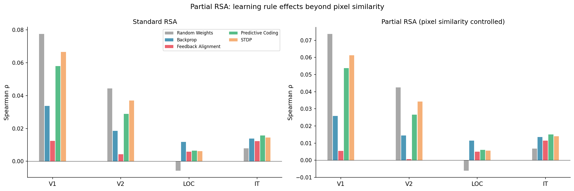
After removing variance explained by pixel-level similarity, all conditions retain their alignment patterns (Table 3). The ordering Random $>$ STDP $>$ PC $>$ BP $>$ FA at V1 is fully preserved, with small and comparable decreases across conditions ($\Delta\approx-0.004$ to $-0.008$). This confirms that the architecture-dominance effect reflects genuine representational structure beyond low-level image statistics.

Table 3: Standard vs. partial RSA at V1 (pixel similarity controlled, $224\times 224$). Partial RSA was computed from a single seed-averaged model RDM rather than averaging partial $\rho$ across seeds, which accounts for minor differences from Table 2 (e.g., Random $\rho_{\text{std}}=0.078$ here vs. $0.076$ in Table 2).

Condition	$\rho_{\text{std}}$	$\rho_{\text{partial}}$	$\Delta$
Random	0.078	0.074	$-0.004$
STDP	0.067	0.061	$-0.005$
PC	0.058	0.054	$-0.004$
BP	0.034	0.026	$-0.008$
FA	0.012	0.005	$-0.007$

Figure 8: Partial RSA controlling for pixel similarity. Left: standard RSA scores. Right: partial Spearman $\rho$ after regressing out the pixel-similarity RDM. The rank ordering of conditions is preserved after pixel control, and the decrease in $\rho$ is small and comparable across conditions ($\Delta\approx-0.005$ to $-0.008$ at V1).

4.9 Filter Analysis

Figure 9: Conv1 filter analysis for all five conditions. (a) First 16 Conv1 filters per learning rule. All conditions show color-opponent patch structure rather than oriented Gabor patterns, consistent with CIFAR-10 training at $224\times 224$. (b) Gabor-peakedness (FFT spectral peak-to-mean ratio): BP $2.00\pm 0.52$, FA $1.82\pm 0.36$, STDP $1.79\pm 0.47$, PC $1.73\pm 0.45$, Random $1.73\pm 0.45$. Differences are small relative to within-rule variability.

Conv1 filters from all five conditions exhibit color-opponent patch structure rather than oriented Gabor-like patterns, consistent with CIFAR-10 training. The Gabor-peakedness score (FFT spectral peak-to-mean ratio) is highest for BP ($2.00\pm 0.52$), followed by FA ($1.82\pm 0.36$), STDP ($1.79\pm 0.47$), PC ($1.73\pm 0.45$), and Random ($1.73\pm 0.45$). The differences are small relative to within-rule variability and standard deviations overlap substantially across all conditions, indicating that no learning rule produces markedly more Gabor-like filters than random initialization at this scale.

5 Discussion

Architecture as the primary driver of early alignment. Our most striking finding is that an untrained CNN exceeds backpropagation at V1 ($\rho=0.076$ vs. $0.034$, $\Delta\rho=+0.044$, $p<0.001$). This goes beyond the observation of Saxe et al., (2011) that random networks have non-trivial visual structure: in our setup, the convolutional inductive biases (local connectivity, ReLU, pooling) are not merely comparable to BP but produce higher early visual alignment. This suggests that, at least for small CNNs trained on CIFAR-10, backpropagation on a classification objective moves early-layer representations away from V1-like structure. Whether this holds at larger scales (e.g., ResNet-50 on ImageNet) remains to be tested. Among trained rules, STDP ($\rho=0.064$) and PC ($\rho=0.056$) preserve more V1-like structure than BP, consistent with the idea that local unsupervised learning retains more of the architectural inductive bias (Olshausen and Field,, 1996).

Learning rules converge at higher areas. At LOC, only BP significantly exceeds the random baseline, but differences among trained rules are small and non-significant after FDR correction. At IT, all five conditions converge completely. This convergence may reflect a genuine property of abstract categorical representations, but is also consistent with a capacity limitation: our small CNN trained on 8,000 CIFAR-10 samples may simply lack the representational power to differentiate at higher layers. Prior work with larger models suggests that BP-trained networks have a systematic IT advantage (Schrimpf et al.,, 2020); whether this advantage reflects the learning rule or the additional model capacity remains an open question. We note that the noise ceiling at IT is also the lowest of all ROIs (upper bound: 0.07), leaving limited room for any condition to differentiate — it is possible that true differences exist but are unresolvable given the fMRI signal quality at this ROI and sample size ($N=3$).

PC and STDP as biologically plausible routes to V1 alignment. PC ($\rho=0.056$) and STDP ($\rho=0.064$) outperform BP ($\rho=0.034$) at V1—the cortical area where biological plausibility is most constrained by known physiology. Both rules use local updates without global error signals, suggesting that local computation preserves more of the architectural inductive bias that underlies V1-like representations. This is consistent with the theoretical argument that PC approximates BP under certain conditions (Whittington and Bogacz,, 2017), but the superior V1 alignment of PC and STDP over BP suggests they may be more appropriate models of early visual cortex than BP.

FA consistently lowest. FA produces the lowest alignment among trained rules at V1, V2, and LOC, significantly below all other conditions at V1/V2 ($p<0.001$), despite achieving 39% task accuracy. This is consistent with random feedback filters disrupting the representational structure that convolutional architecture provides, though we cannot rule out that this reflects an optimization artifact specific to FA in convolutional networks rather than a fundamental incompatibility. At V2, FA’s partial RSA score drops to near zero ($\rho_{\text{partial}}=0.001$, $p=0.755$), indicating that essentially none of FA’s V2 alignment survives pixel-similarity control. This result may be specific to CNNs, where spatial structure in feature maps interacts poorly with random feedback filters (Lillicrap et al.,, 2016).

Dissociation between task performance and brain alignment. Task accuracy and brain alignment are dissociated throughout the hierarchy in our small-scale setting. At V1, the untrained baseline (10% accuracy) exceeds BP (82% accuracy), and STDP (63%) and PC (57%) both outperform BP despite lower task performance. At IT, all rules converge regardless of accuracy. This suggests that, at least for small CNNs trained on CIFAR-10, the relevant axis is not “how well does it classify” but “what representational structure does the objective induce at each layer.” Whether this dissociation persists at ImageNet scale, where task-optimized models achieve substantially higher Brain-Score alignment (Schrimpf et al.,, 2020), remains an open question.

Implications. Our results carry two concrete methodological messages. For computational neuroscience: studies comparing trained models to brain data must always include an untrained baseline with the same architecture. Without this control, architecture effects are confounded with learning effects—our data show this confound can be essentially complete at V1. For machine learning: the inductive biases of the convolutional architecture (local connectivity, weight sharing, ReLU, pooling) are more important than the weight-update rule for early-layer feature representations. When designing architectures for brain-inspired AI, the structural priors deserve as much attention as the learning algorithm.

5.1 Limitations

Several limitations bound our conclusions. (1) All models were trained on CIFAR-10 using a small custom CNN, far below the scale at which ResNet-50 or ViT models achieve competitive Brain-Score results. The small architecture limits representational capacity and may explain the IT convergence. (2) We have only 3 subjects, with sub-03 showing consistently weak signal; our core findings are driven by sub-01 and sub-02. Replication on a larger dataset (e.g., Natural Scenes Dataset, $N=8$) would strengthen generalizability. (3) STDP was applied to static images via Poisson spike trains, discarding the temporal dynamics that STDP was designed to exploit. (4) The best-layer-per-ROI analysis reveals that FC1 sometimes produces higher V1 alignment than Conv1, complicating the anatomical mapping assumption. (5) Gabor-peakedness scores show no significant differences across learning rules, but this metric captures only a coarse proxy for V1-like filter structure. (6) Bootstrap CIs resample stimulus pairs rather than stimuli, which may underestimate uncertainty. (7) We use a single dataset (THINGS-fMRI); cross-dataset replication would strengthen all claims. (8) Models were trained at $32\times 32$ resolution but evaluated at $224\times 224$; random filters are approximately scale-invariant while trained filters are optimized for $32\times 32$ statistics, which may partly contribute to the random baseline’s advantage at V1.

6 Conclusion

We presented a systematic RSA comparison of four learning rules plus an untrained baseline at $224\times 224$ resolution, averaged across 5 seeds, against the THINGS-fMRI benchmark. In our small-scale setup, the learning rule has little effect on cortical alignment: architecture dominates early visual representations (V1/V2), where the untrained baseline exceeds all trained rules, and all rules converge at higher areas (IT), with no reliable pairwise differences—though this convergence may partly reflect model capacity limitations. Only LOC shows a selective learning effect, where BP alone reliably exceeds the random baseline. Among trained rules, PC and STDP preserve more V1-like structure than BP, suggesting that local unsupervised learning retains architectural inductive biases that global error signals may disrupt. FA consistently produces the lowest alignment despite meaningful task accuracy. These results suggest that, at least at this scale, the search for biologically plausible learning rules should focus on preserving architectural inductive biases at early areas, rather than optimizing for task performance. Whether these findings generalize to larger architectures trained on richer datasets remains an important open question.

Code Availability

Code and results: https://github.com/nilsleut/learning-rules-rsa.

References

- Bi and Poo, (1998) Bi, G.-q. and Poo, M.-m. (1998). Synaptic modifications in cultured hippocampal neurons: dependence on spike timing, synaptic strength, and postsynaptic cell type. Journal of Neuroscience, 18:10464–10472.
- Crick, (1989) Crick, F. (1989). The recent excitement about neural networks. Nature, 337:129–132.
- Gifford and Cichy, (2022) Gifford, A. T. and Cichy, R. M. (2022). THINGS-fMRI: A large-scale dataset of fMRI brain responses to 22,248 images from the THINGS object concept database. NeuroImage, 264:119628.
- Hebart et al., (2019) Hebart, M. N., Dickter, A. H., Kidder, A., Kwok, W. Y., Corriveau, A., Van Wicklin, C., and Baker, C. I. (2019). THINGS: A database of 1,854 object concepts and more than 26,000 naturalistic object images. PLOS ONE, 14:e0223792.
- Kriegeskorte et al., (2008) Kriegeskorte, N., Mur, M., and Bandettini, P. (2008). Representational similarity analysis – connecting the branches of systems neuroscience. Frontiers in Systems Neuroscience, 2:4.
- Lillicrap et al., (2016) Lillicrap, T. P., Cownden, D., Tweed, D. B., and Akerman, C. J. (2016). Random synaptic feedback weights support error backpropagation for deep learning. Nature Communications, 7:13276.
- Lillicrap et al., (2020) Lillicrap, T. P., Santoro, A., Marris, L., Akerman, C. J., and Hinton, G. (2020). Backpropagation and the brain. Nature Reviews Neuroscience, 21:335–346.
- Olshausen and Field, (1996) Olshausen, B. A. and Field, D. J. (1996). Emergence of simple-cell receptive field properties by learning a sparse code for natural images. Nature, 381:607–609.
- Rao and Ballard, (1999) Rao, R. P. N. and Ballard, D. H. (1999). Predictive coding in the visual cortex: a functional interpretation of some extra-classical receptive-field effects. Nature Neuroscience, 2:79–87.
- Saxe et al., (2011) Saxe, A. M., Koh, P. W., Chen, Z., Bhand, M., Suresh, B., and Ng, A. Y. (2011). On random weights and unsupervised feature learning. In Proceedings of the 28th International Conference on Machine Learning.
- Schrimpf et al., (2020) Schrimpf, M., Kubilius, J., Hong, H., Majaj, N. J., Rajalingham, R., Issa, E. B., Kar, K., Bashivan, P., Prescott-Roy, J., Schmidt, K., Yamins, D. L. K., and DiCarlo, J. J. (2020). Brain-Score: Which artificial neural network for object recognition is most brain-like? bioRxiv.
- Truzzi and Cusack, (2025) Truzzi, A. and Cusack, R. (2025). Neural responses in early visual cortex are well predicted by random-weight CNNs. bioRxiv.
- Whittington and Bogacz, (2017) Whittington, J. C. R. and Bogacz, R. (2017). An approximation of the error backpropagation algorithm in a predictive coding network with local Hebbian synaptic plasticity. Neural Computation, 29:1229–1262.
- Yamins and DiCarlo, (2016) Yamins, D. L. K. and DiCarlo, J. J. (2016). Using goal-driven deep learning models to understand sensory cortex. Nature Neuroscience, 19:356–365.