Single-Satellite Quantum Repeater Performance Analysis

Abstract

Space-based entanglement distribution has the potential to extend the range of quantum communication beyond that achievable through optical fibres that are constrained by exponential losses. Quantum repeaters have been proposed to mitigate the effects of channel losses for both fibre and satellite networks. Although quantum repeaters can improve entanglement distribution efficiency, the rate is constrained by classical communication latency in the entanglement swapping process. Direct dual downlink entangled pair distribution does not suffer such a latency restriction, hence can “brute force” the problem of high dual channel loss through increased source rate. Hence, the comparative requirements of direct pair distribution versus quantum repeater satellites are important for the design and deployment of space-based entanglement distribution systems. Here, we consider the simplest case of a single satellite establishing entanglement between two ground stations, comparing the performance of direct dual downlink to that of a space-based quantum repeater for general overpass geometries. We also study the long-term entanglement distribution performance for different ground station pairs and determine altitudinal dependence. Finally, we study the fidelity distribution of a satellite repeater system through Monte Carlo modelling of waiting times and rate statistics, exploring the effect of quantum memory capacity, decoherence rates, and operational policies. These results will inform mission design for future space-borne quantum repeater nodes, as well as requirements on space-based memory platforms.

1 Introduction

Emerging quantum technologies offer the ability to establish provably secure cryptographic keys BennettQuantumCryptography ; ShorPreskillSecurityProof ; ScaraniSecuirty.81.1301 , improve sensing capabilities GiovannettiMetrology ; DegenQuantumSensing , enable precise clock synchronisation ShiClockSynchronisation , and computational speed-up for certain problems ShorFactoring . Robust and reliable distribution of quantum entanglement is essential for the implemention of many of these technologies. Optical fibre is limited by exponential photonic loss scaling with distance PirandolaAdvancesInQuantumCryptography , limiting their viability for direct entanglement distribution to a few hundred kilometres. This range can be extended using quantum repeaters BriegelQRs , but long-range fibre links still face implementational challenges due to the requirements for close spacing, number, and placement of repeater stations between end-nodes.

Following landmark experiments by the Micius mission miciusExperiemntsInSpace there has been much interest in space quantum communications to extend the range of entanglement distribution Sidhu_2021AdvancsIn ; belenchia2022quantum ; koudia2024spacebasedquantuminternetentanglement . Satellite links exploit the more benign inverse square diffraction loss scaling and vacuum propagation for the majority of a space-Earth link and have advantages of access to moving platforms and remote areas where fibre links may be impractical. Micius was successful in distributing entanglement between ground stations over 1000 km apart, though direct pair distribution losses led to a received rate of $\sim 1$ pairs s^-1 from $5.9\times 10^{6}$ pairs s^-1 sent.

Satellite quantum repeaters with quantum memories, are a promising platform for distributing entanglement at large scales gundoganProposalSpaceMemories2020 ; fittipaldiEntSwappingInOrbit2024 ; LiorniQRsInSapce ; gundoganJasBeyondLOS . Quantum repeaters greatly increase the efficiency of distributing entanglement at the cost of introducing communication latency which impacts the distribution rate. Direct transmission does not incur such latencies, hence their overall entanglement distribution rate can be increased through “brute-force” by simply using a higher source rate. Single-satellite direct dual-downlink (DDDL) entanglement distribution (a la Micius) is the most feasible to implement in the near term, but there are growing efforts to develop space quantum memories and repeaters as a path to a longer-term solution. Thus it is important to understand their respective resource requirements, performance characteristics, and the cross-over point between the two approaches. In this work, we focus on a link consisting of a single satellite and two optical ground stations (OGSs), providing a systematic exploration of the performance of these dual downlinks for general overpass geometries. We also develop a Monte Carlo model of satellite repeater memory allocation and entanglement swapping policies and fidelities.

We organise this work as follows. In Section 2 we: provide background and context to our work; describe our dual-downlink channel model and the the entanglement distribution protocols that we consider; and outline the Monte Carlo simulation method of quantum memory/repeater operation for determining entanglement fidelity statistics. In Section 3 we present our results of: the per-overpass entanglement distribution volume of a satellite operating with and without quantum memories, comparing the performance of each under varying overpass geometry; the estimate of the average total number of entangled pairs distributed over the course of a year; waiting times and distributed entanglement fidelities for a selection of overpasses from the Monte Carlo analysis. We conclude in Section 4 by identifying avenues of future research that would build on this work.

Figure 1: Single Satellite – Two OGS Overpass Geometry. A single satellite simultaneously communicates with Alice ($\text{OGS}_{\text{A}}$ ) and Bob ($\text{OGS}_{\text{B}}$ ) in a single satellite quantum repeater (SSQR) configuration. We consider a satellite in a circular orbit of altitude $h$. The great-circle separating A and B of arc-length $d$ is denoted the OGS baseline. We choose to parameterise the overpass geometry by the intersection of the satellite ground track with the OGS baseline, defined by the crossing angle ($\phi$) and offset ($\Delta$) relative to the midpoint position (an alternative choice would be to parameterise each single downlink by the minimum ground track offset to each OGS, $\{d_{min}^{A},d_{min}^{B}\}$). The slant distances to the OGS’s $\{L_{A}(t),L_{B}(t)\}$, and the local elevations $\{\theta_{A}(t),\theta_{B}(t)\}$ vary during the overpass. Entanglement distribution is possible when the satellite is above the minimum elevation $\theta_{\text{min}}$ for both A and B at the same time. An overpass is defined as the period for which this dual-visibility criterion is met. In the direct dual downlink (DDDL) configuration, the satellite transmits pairs of entangled photons simultaneously, one photon to each OGS. For a single satellite repeater (SSQR), the satellite has two independent sets of an entanglement source and quantum memory to establish an entangled link with each OGS, together with an entanglement swapping mechanism.

2 Preliminaries and Methods

In this section we describe the methodology and protocols employed. We describe the situation of a single satellite communicating with 2 OGSs through quantum optical channels and define a parameterisation of general overpass geometries. The two methods of entanglement distribution studied are introduced, together with the estimation procedure of the short and long-term performance. We finally cover the modelling and entanglement fidelity estimation of the quantum repeater protocol under a memory and swapping policy. In this preliminary investigation, we will not consider weather effects or time varying background light alongside other simplifications of the problem such as identical OGSs and night operations.

2.1 Dual-Downlink Overpass Channel Loss

The single-satellite 2-OGS configuration is the simplest space-based entanglement distribution topology. The most general dual-downlink overpass geometry is shown in Fig. 1 and can be parameterised by the pair of variables $\{\Delta,\phi\}$ sidhu2026operational . We are interested in determining the effect of overpass geometry on the ability of the satellite to distribute entanglement to better understand future mission and constellation performance and design considerations. The entanglement distribution performance will be determined by the optical losses in each satellite-OGS channel. We model each link as for a single-satellite one OGS configuration sidhu2021finitekeyeffectssatellite ; sidhuFiniteResource (See Appendix A). The slant distances $\{L_{A}(t),L_{B}(t)\}$ and elevations $\{\theta_{A}(t),\theta_{B}(t)\}$ determine the transmittances $\eta_{A}(t)$ and $\eta_{B}(t)$ of the $\text{OGS}_{\text{A}}$ and $\text{OGS}_{\text{B}}$ downlinks, respectively (see Appendix B4 for details). For the DDDL configuration, the effective dual channel transmittance is $\eta_{AB}=\eta_{A}\eta_{B}$, whereas for SSQR it scales as $\sim\min\{\eta_{A},\eta_{B}\}$.

2.2 Satellite Entanglement Distribution

We describe the two entanglement distribution protocols that we consider corresponding to: direct dual downlink (DDDL) in which the satellite is equipped only with an entangled pair source (EPS) and no quantum memory; a single satellite repeater (SSQR) using the Sender-Receiver protocol Jones_2016 . Other quantum repeater protocols, for example All-photonic azuma2015all , but we relegate their treatment to future work.

2.2.1 Direct Dual-Downlink.

In DDDL, the satellite is only equipped with an onboard entangled photon source (EPS). The satellite generates entangled photon pairs and sends one photon of each pair to Alice and Bob. If the EPS produces entangled photons at a rate $R_{\text{EPS}}$, then the instantaneous pair distribution rate (PDR) is given by

$$R^{\text{DDDL}}(t)=\eta_{A}(t)\eta_{B}(t)R_{\text{EPS}}^{DDDL}.$$ (1)

For simplicity, we consider a deterministic source pan2026quantum . In practice, EPSs for satellite deployment (e.g. villar2020entanglement ; mccarthy2025compact ) are currently based on spontaneous parametric down conversion (SPDC), either pulsed or continuously pumped, where the production of entangled pairs becomes probabilistic and the performance is inferior to a deterministic source of the same average pair production rate. Hence our model provides an upper bound to the performance of DDDL. The pair distribution volume (PDV) for DDDL can be calculated by integrating Eq. 1 over the duration of the overpass, similarly for SSQR. DDDL quantum key distribution has been studied in wang2026scalability ; sidhu2026operational .

2.2.2 Satellite Quantum Repeater Entanglement Distribution.

Figure 2: Single Satellite Quantum Repeater. 1) Each downlink independently establishes an entangled pair the satellite quantum memory and an OGS: 1a) An EPS generates an entangled pair of photons, one photon is in a satellite quantum memory mode slot (alternatively, a DLCZ-type-entanglement source duan2001long can be used); 1b) The other photon is sent to the OGS with time-of-flight $\tau_{A,B}$; 1c) The OGS notifies the satellite of transmission success/failure, with return signal time-of-flight $\tau_{A,B}$; 1d) In the case of transmission failure, the memory is reset and a new entanglement distribution attempt is made. If the photon was received by the OGS, the protocol proceeds to the next stage. 2) Once a link has been successful in establishing an entangled pair, it either waits for the other link to succeed, if it has not already been successful. 3) Once both links are ready, the satellite performs entanglement swapping to link the two OGSs. We assume a success probability of 50% for a linear optical Bell State Measurement (BSM). 4) The swap result is conveyed to the OGSs allowing them to perform corrective operations or discard the attempt in the case of failure. The latency of this stage has no impact upon the operational rate. Each link can be parallelised using multiply memory mode slots, providing a linear increase in the PDR.

Quantum repeaters have been proposed to address the challenge of distributing entanglement over high loss channels typical of long distance links BriegelQRs . This is achieved by splitting a large link into multiple smaller sublinks over which quantum transmission is possible and connecting them using quantum memories, classical communications and entanglement swapping azumaRepeatersReview2023 ; munroInsideRepeaters2015 in order to overcome the direct transmission limit. Satellite links, although possessing a much more favourable loss scaling than fibre links, can still suffer high losses. For example, the Micius dual-downlink experiments reported losses of the order of $27\ \text{dB}$ or greater per downlink, or of the order of $>55\text{dB}$ for the combined DDDL link loss. Satellite quantum memory repeaters have been proposed to improve the performance of the satellite for quantum communications gundoganProposalSpaceMemories2020 .

The basic operation of a repeater satellite is shown in Fig. 2. Repeater protocols require classical communication between the satellite and each OGS, introducing an unavoidable communication latency leading to two important practical considerations. First, there is an immediate constraint on the minimum lifetime of a candidate memory platform. These latency times are determined by the two-way photon transit times which are on the order of ms for satellite in low Earth orbit (LEO). Second, the latency also imposes a bottleneck on the rate at which entanglement distribution can be attempted. This reduction to the PDR is compounded by the fact that the Bell state measurement (BSM) that performs entanglement swapping will typically only succeed with a probability $p_{\text{BSM}}$ BSMRefdoi:10.1126/sciadv.adf4080 . Although future technology may allow for deterministic BSMs, here we assume a conventional BSM and success probability of $50\%$.

2.2.3 Initial Comparison of DDDL and SSQR.

To illustrate the potential benefit a quantum memory could offer entanglement distribution, consider the case of static symmetric links with transmittance $\eta=10^{-3}$ to each of Alice and Bob. If the satellite has an onboard entangled pair source (EPS) with the Micius source rate of $5.9\times 10^{6}\ \text{ pairs s}^{-1}$, the DDDL distribution rate to Alice and Bob is, $10^{-3}\cdot 10^{-3}\cdot 5.9\times 10^{6}=5.9\ \text{pairs s}^{-1}$. With an unconstrained number of memory slots and using the same entanglement source rate, the satellite establishes pairs with Alice and Bob individually at a rate, $R_{\text{A,B}}=10^{-3}\cdot 5.9\times 10^{6}=5900\ \text{pairs s}^{-1}$. If the BSM succeeds with probability $p_{\text{BSM}}$, then the SSQR rate is, $p_{\text{BSM}}\times 5900\ \text{pairs s}^{-1}$, which is $3$ orders of magnitude higher than the rate without memories, up to $p_{\text{BSM}}$. This advantage arises because having memories on board removes the need for simultaneous success in dual-downlink transmission, i.e. splitting the simultaneous dual downlink into two independent single downlinks, leading to the distribution rate scaling as $\eta$ for SSQR compared with $\eta^{2}$ for DDDL.

2.2.4 Memory Capacity Impact on SSQR Rate.

The above assumes that the memory was not subject to any constraints in terms of its capacity and lifetime. In practice, quantum memories are limited in the total number of memory modes or slots. This affects the rate at which entanglement distribution can be attempted. For a single mode, since distribution can only be reattempted following classical signalling from the ground stations, the rate at which entanglement distribution can be attempted is,

$$R_{\text{EPS}}^{\text{SSQR}}=\frac{1}{2\tau_{A,B}}=\frac{c}{2L_{A,B}}.$$ (2)

For a low-Earth orbit (LEO) altitude $h=500\ \text{km}$, this round trip time has a minimum value of $\sim 3.3\ \text{ms}$ when the satellite is at zenith (i.e. directly above an OGS), leading to a maximum attempt rate of $R_{\text{EPS}}^{\text{SSQR}}\lesssim 300\ \text{s}^{-1}$. For $\eta=10^{-3}$, the rate at which entanglement can be established on a single link would then only be $0.3\text{ pairs s}^{-1}$. However, this process can by multiplexed with multiple satellite memory modes leading to a linear rate scaling. Going forward, we no longer assume that the satellite has an unconstrained number of memory slots but impose a finite capacity $N_{\text{sat}}$, we do not impose any limit on the OGSs. We note that the EPS rate only needs to be the same as the satellite-OGS link attempt rate, potentially relaxing the requirements for photon and quantum memory bandwidth by a considerable amount.

We consider the Sender-Receiver protocol Jones_2016 where the satellite assigns $N_{A}$ and $N_{B}$ modes of its memory to each of Alice and Bob ($N_{A}+N_{B}=N_{\text{sat}}$), respectively. The average rate ($R_{A,B}$) of entanglement generation to each OGS and the overall entanglement distribution rate after entanglement swapping ($R^{\text{SSQR}}$) are,

$$R_{A,B}=\frac{1}{2\tau_{A,B}}\sum_{k=1}^{N_{A,B}}\binom{N_{A,B}}{k}\eta_{A,B}^{k}(1-\eta_{A,B})^{N_{A,B}-k}k,\quad R^{\text{SSQR}}=p_{\text{BSM}}\text{ min}\{R_{A},R_{B}\}.$$ (3)

Note that we do not include the effect of any processing time required on the satellite or ground station in Eq. 3, including the time to latch photons into the ground station memory and perform the BSM, valid in the limit that the photon transit times are dominant.

From the instantaneous PDR, the single overpass pair distribution volume (PDV) is,

$$N_{\text{PDV}}^{\text{DDDL,SSQR}}=\int_{t_{\text{start}}}^{t_{\text{end}}}\ R^{\text{DDDL,SSQR}}(t)\ dt,$$ (4)

where $t_{\text{start}}$ and $t_{\text{end}}$ denote the times between which the satellite is in simultaneous view above the minimum elevation at each OGS. In principle, a SSQR could begin to load up the memory slots of the first OGS in view prior to simultaneous visibility, but we neglect this possibility to simplify the model. The extreme case would be the use of long-duration quantum memories to courier entanglement between distant OGSs in a time-delayed quantum repeater protocol gundoganJasBeyondLOS .

A natural question would be how best to assign the memory slots to each of the Alice and Bob downlinks. The most general scheme would be where these allocations dynamically vary with time during an overpass and are adjusted based on link parameters, i.e. $N_{A}=N_{A}(t)$ and $N_{B}(t)=N_{\text{tot}}-N_{A}(t)$, as considered in fittipaldiEntSwappingInOrbit2024 . Since dynamical memory allocation between downlinks may introduce experimental complexity, and to simplify the analysis, we consider a static memory allocation for the duration of an overpass, though this can vary on an overpass to overpass basis. The simplest choice is $N_{A}=N_{B}=N_{\text{tot}}/2$, though this may not be optimal for a given overpass geometry. For example, if an overpass passes directly overhead Alice and not Bob, meaning that $\eta_{A}(t)>\eta_{B}(t)$ throughout, then the PDV can be improved by assigning the $OGS_{B}$ link more onboard memory to compensate for its higher link loss. This can be understood from Eq. 3 where the overall $R^{\text{SSQR}}$ is maximised when the individual satellite-Alice $R_{A}$ and satellite-Bob $R_{B}$ rates are equalised . We therefore consider the case where the satellite employs an optimal static allocation of its memory, chosen to maximise the per-pass PDV. This would offer a balance between improving the distribution rates compared to an equal split without introducing extra experimental complexity.

The communications latency that repeater protocols suffer from is reflected in the $1/2\tau$ term in Eq. 2 which DDDL does not suffer. A memory equipped satellite will therefore only outperform DDDL when there is sufficiently high memory capacity to compensate for this latency. We define the crossover capacity, $N_{c}$, as the memory capacity required for SSQR to match DDDL performance. One could consider the instantaneous $N_{c}(t)$ corresponding to setting $R_{\text{DDDL}}(t)=R_{\text{SSQR}}(t)$, though here we consider $N_{c}$ on a per-overpass basis where $N_{\text{PDV}}^{\text{DDDL}}=N_{\text{PDV}}^{\text{SSQR}}$. The crossover capacity has direct relevance for requirements on space-borne memory platforms and gauging the feasibility of candidate platforms.

2.3 Long-term PDV

The per-overpass PDV can depend on the overpass geometry that varies from overpass to overpass. Long-term term entanglement distribution performance is a more representative metric. We consider the expected annual PDV for a Noon-Midnight Sun synchronous orbit (SSO), assuming night-time only operation. We will approximate an SSO by a polar orbit, valid for OGS locations away from the North and South poles sidhu2021finitekeyeffectssatellite . For a circular polar satellite (Fig. 3), overpasses occur along a meridian of fixed longitude $\gamma$. The prime meridian can be taken as the OGS baseline midpoint. The crossing point of the satellite ground track will define an overpass geometry $\Delta_{\gamma}$ and $\phi_{\gamma}$, and a corresponding per-pass PDV, $N_{PDV}(\Delta_{\gamma},\phi_{\gamma})=N_{PDV}(\gamma)$ pairs.

Over the course of the year, the set of $\gamma$ for each orbit can considered to be uniformly and randomly distributed, assuming that there is no Earth synchronism (some constellation designs do employ simultaneous Sun and Earth synchronism mazzarella2020quarc ). We note that many orbits with longitude $\gamma$ will result in $N_{PDV}(\gamma)=0$ if the ground track does not approach close enough to both OGSs simultaneously. The average PDV per orbit, $\bar{N}_{\gamma}$, can be found by averaging over $\gamma$,

$$\bar{N}_{\gamma}=\frac{1}{2\pi}\int_{0}^{2\pi}N_{PDV}(\gamma)\ d\gamma.$$ (5)

Scaling $\bar{N}_{\gamma}$ by the number of overpasses in a year ($N_{\text{annual-orbits}}$) then gives an estimate of the total average annual PDV, $\bar{N}_{\text{year}}$. As illustrated in Fig. 3, overpasses can be characterised as having either a North-South or South-North trajectory. For an SSO satellite, which can be approximated as being polar, only one of these will occur at night. The assumption that entangled pair distribution only occurs on the midnight overpass of a Noon-Midnight SSO can be incorporated into the model by only considering overpasses with $0\leq\phi_{\gamma}\leq\pi$, for example. This restriction enforces that only either North-South or South-North overpasses are counted.

Figure 3: Expected Annual PDV. A polar orbit satellite, in the absence of Earth synchronism, will cross the OGS baseline great circle at randomly distributed longitudes. We only consider the North to South crossings, assuming these occur at local midnight for a noon-midnight SSO for which the polar orbit approximates. For convenience, we can take the prime meridian to be the longitude of the OGS baseline midpoint, the orbital angle is denote $\gamma$. At each crossing point, the overpass geometry is $\{\Delta_{\gamma},\phi_{\gamma}\}$, hence PDV is then a function of $\gamma$. Over the course of year, the expected average can be determined from the integral of $N_{PDV}(\gamma)$ with respect to $\gamma$, suitably normalised and proportional to the number of orbits. Note that $N_{PDV}$ can be positive for crossing points outside of the OGS baseline (e.g. left most crossing point) if there is sufficient line of sight.

2.4 Fidelity of Distributed Entanglement

In addition to the number of entangled pairs is it also important to consider the quality of the distributed entanglement, for example as quantified by entanglement measures 10.5555/2011706.2011707 ; Horodecki_2009QuantumEntanglement . Entanglement measures are typically defined in the asymptotic limit and quantify how well a state can be used for a certain operational task. However, measures defined in this way are typically computationally intractable and are less useful for the characterisation of a small numbers of states that will be typical for near-term satellite quantum networks.

To quantify the quality of the entangled pairs distributed by the satellite we choose the single-copy entanglement fidelity of a 2-qubit state $\hat{\rho}_{AB}$,

$$F=_{AB}\bra{\Phi}\hat{\rho}_{AB}\ket{\Phi}_{AB},$$ (6)

where $\ket{\Phi}_{AB}$ is a maximally entangled state of 2 qubits. Without loss of generality, we choose the maximum overlap over all maximally entangled states, else we can perform a local unitary to maximise the overlap of $\hat{\rho}_{AB}$ with a fixed Bell state $\ket{\Phi^{+}}_{AB}=\frac{1}{\sqrt{2}}\left(\ket{00}+\ket{11}\right)_{AB}$. The fidelity is a suitable metric to use in the context of finite block sizes. It allows us to evaluate the quality of the distributed pairs individually without appealing to an asymptotic limit. A fidelity of $1$ represents perfect entanglement with no noise, and it can be shown that if a two-qubit state has $F>1/2$ then this implies that it is entangled horoSingleFractionReference . Furthermore, different quantum technology applications typically have fidelity thresholds (see e.g. de_Forges_de_Parny_2023 Table $1$).

To simplify the analysis, we assume that the satellite produces perfect Bell pairs on board and that any fidelity loss due to transmission through the atmosphere and subsequent reception and storage on the ground is negligible (ignoring background light). Under these assumptions the only source of fidelity degradation is decoherence of photon stored in the satellite quantum memory whilst awaiting the “success” signal from the OGSs. Different quantum memory types have varying storage and retrieval characteristics, here we will assume that storage and retrieval efficiency is ideal but introduce a non-zero dephasing rate of a stored qubit state $\hat{\varrho}$ modelled as Walln_fer_2022 ,

$$\hat{\varrho}\mapsto(1-\lambda(t))\hat{\varrho}+\lambda(t)\hat{Z}\hat{\varrho}\hat{Z},\qquad\lambda(t)=\frac{1-\exp(-t/\tau_{\text{mem}})}{2}$$ (7)

after storage time $t$, $\tau_{mem}$ is the $1/e$ dephasing time of the memory, and $\hat{Z}$ is the Pauli Z-operator acting the stored qubit.

The repeater satellite performs entanglement swapping on qubits stored in its memory after Alice and Bob each confirm successful photon transmission. If the satellite-Alice and satellite-Bob memory qubits have been stored for times $t_{A}$ and $t_{B}$ respectively, then the Alice-Bob pair after swapping can be shown (Appendix D) to be a Bell-diagonal state with fidelity

$$F(t_{A},t_{B})=\lambda(t_{A})\lambda(t_{B})+(1-\lambda(t_{A}))(1-\lambda(t_{B})).$$ (8)

The development of memories that combine long lifetimes with on-demand photon emission and high levels of multimodality is of critical importance for the development of scalable repeater applications. Storage times on the order of microseconds have been reported mustafaMicrosecondLifetime , as well as times of $1\ \text{ms}$, through the use of clock states robust against decoherence caused by residual magnetic fields ZhaoClockStates . Dynamical decoupling techniques have allowed for storage times of six hours in rare-earth memories ZhongSixHourCoherence . Storage of $50$ and $100$ simultaneous modes has been demonstrated in atomic frequency comb memories AFC50100Modes , with capacities of $59$ RE59cap and $1650$ AFC1650 demonstrated in rare-earth memories. However, no platform that combines on-demand emission, long storage times, high degrees of multiplexing and the low size, weight, and power (SWaP) requirements that would be necessary for satellite deployment have yet been demonstrated.

2.5 Monte Carlo Model of Quantum Repeater Operation

The fidelity in Eq. 8 is non-linear in the waiting times hence it is therefore not sufficient to just calculate average waiting times to establish the mean fidelity. We are also interested in the statistical distribution of fidelities as this will inform future work on purification and swapping strategies. A complete characterisation requires accessing the waiting time statistics, motivating our use of Monte Carlo (MC) methods. Although computationally expensive, MC methods are well suited to modelling complex probabilistic systems. They are a natural choice for modelling quantum repeaters and have been used in previous research (see e.g. Walln_fer_2024 ; niu2023all ).

In the MC model, we keep track of the internal state of the satellite’s onboard quantum memory throughout the overpass. The loading and swapping time stamps of each of the stored photons on board the satellite are recorded, from the waiting time the final fidelity of the distributed pairs between Alice and Bob are calculated from Eq. 8.

2.5.1 Memory Management and Swapping Policies.

(a) At the start of a round, the satellite may have memory qubits leftover from a previous time step. For this example, these are in the Alice register with current waiting time $\tau_{1}$.

(b) Entanglement distribution is attempted and after successful transmission is confirmed, fresh memory qubits have waiting times equal to the round-trip delay. The youngest qubits are used for swapping.

(c) Following the swapping the satellite trims the memory by discarding the oldest qubits down to the buffer size (2 in this example).

(d) Following swapping and trimming this process is repeater, with the buffer having been replenished with fresh pairs.

Figure 4: Memory management strategy. The satellite memory is split into separate registers for Alice (Red) and Bob (Blue). The horizontal axis indicates the current waiting of memory qubits and increases moving away from the centre.

There is freedom in how to manage the memory slots on the satellite, namely what to do with excess unpaired stored photons, and the choice of which photons to swap once both links have successes. If a qubit has been stored for too long and has its entanglement with the OGS has degraded, it may be preferable to discard it and attempt to refresh it. If the satellite has multiple qubits that are candidates for swapping, it must decide on which are the most appropriate to use.

To address these considerations, we assume that the satellite swaps pairs as soon as possible and always chooses the youngest (i.e. most recently confirmed) memory qubits to use in a swapping operation. This choice is motivated by the fact that the fidelity of the post-swapping pair decreases as both the Alice and Bob storage times increase. Choosing the most recent memory qubits to use in swapping therefore maximises the fidelity of the resulting pair. After swapping, the satellite trims its memory by discarding qubits in the Alice and Bob registers down to a predetermined buffer size. This memory management strategy is illustrated in Fig. 4.

Instead of a fixed buffer size, the trimming of excess stored qubits could be determined by a cut-off time cutoffs_I_esta_2023 ; Walln_fer_2022 ; cutoff_Rozpedek_2018 , which is a maximum storage time for a state in a quantum memory. Introducing a buffer or a cut-off time serves the same purpose of discarding qubits that have become severely degraded. This frees up memory resources to reattempt entanglement distribution with fresh qubits.

3 Results and Discussion

The effect of a changing overpass on the satellite’s performance is a central consideration of this work. We calculate the per-pass PDV (Section 3.1) of a satellite for different overpass geometries, which allows for an estimation of the memory resources required for a repeater satellite to match DDDL. Different optimal overpass geometries for DDDL and repeater satellites are established. The effect of changing baseline system loss values is also considered, as well as a comparison of a repeater satellite adopting an optimal static and equal split of its memory.

The long-term performance of the satellite is evaluate in terms of the average annual PDV (Section 3.2). This is done for a DDDL satellite with Micius source rate and a repeater satellite with $N_{\text{sat}}=200$, with a baseline system loss of $\eta_{\text{loss}}^{\text{sys}}=25.9\ \text{dB}$. Higher optimal altitudes for the repeater satellite compared to DDDL are shown. The relative benefit of adopting an optimal static memory allocation compared to an equal one is shown to depend on the inclination of the OGS baseline with respect to the equator.

Although the PDV is a useful metric it does not quantify the quality of the distributed pairs. To address this, we impose finite memory lifetimes on the satellite and consider dephasing noise in the quantum memory. Evaluating the quality of the pairs then requires accessing the waiting time statistics of the qubits for which we use a round-based MC model of the repeater satellite. The waiting times for different overpasses and their dependence on $N_{\text{sat}}$ are investigated. We then give the fidelities of the distributed pairs as a function of overpass time, as well as their distribution in the final ensemble held by the OGSs at the end of the overpass, for $\tau_{\text{mem}}=100$ ms. Finally, we evaluate the median fidelity of all distributed pairs for varying $\tau_{\text{mem}}$.

3.1 Per-Overpass PDV

Figure 5: Representative overpass geometries. The dashed circles centred on Alice and Bob show their individual visibility regions. Their overlap defines the dual-visibility region, in which the satellite can attempt to distribute entanglement to the ground stations. The dashed arrows show the ground tracks of the satellite trajectories. Bolded segments are where dual-visibility is satisfied and it is the time intervals corresponding to these that defines an overpass.

(a) Zenith-zenith ($\Delta=0\ \text{km},\phi=0^{\circ}$).

(b) Symmetric ($\Delta=0\ \text{ km},\phi=90^{\circ}$).

(c) Zenith A $90^{\circ}$ ($\Delta=500\text{ km},\phi=90^{\circ}$).

(d) Zenith A $45^{\circ}$ ($\Delta=500\text{ km},\phi=45^{\circ}$).

Figure 6: Individual channel losses for the representative overpasses: (a) Zenith-zenith, (b) Symmetric, (c) Zenith A $90^{\circ}$ and (d) Zenith A $45^{\circ}$. The $t=0$ s point is when the satellite’s ground track intersects the OGS baseline or the mid-point for the Zenith-zenith overpass. The dotted line indicates $\eta^{\text{sys}}_{\text{loss}}$ where the single-OGS link loss is at its minimum possible value.

Description	Parameter	Value
OGS baseline length	$d$	$1000$ km
Orbital altitude	$h$	$500$ km
Lifetime of satellite memories	$\tau^{\text{sat}}_{\text{mem}}$	$\infty$
Minimum elevation angle for visibility	$\theta_{\text{min}}$	$10^{\circ}$
Bell state measurement success probability	$p_{\text{BSM}}$	$\frac{1}{2}$
DDDL entangled pair source rate	$R_{\text{EPS}}^{\text{DDDL}}$	$5.9\times 10^{6}$ pairs s-1
Source wavelength	$\lambda$	$780$ nm
Atmospheric transmittance at zenith	$\eta_{atm}$	0.79
Transmitter Aperture diameter $T_{X}$	$D_{t}$	$100\ \text{mm}$
Transmitter Gaussian beam waist	$w_{0}$	$45\ \text{mm}$
Receiver aperture diameter $R_{X}$	$D_{r}$	$1000\ \text{mm}$
Intrinsic loss	$\eta_{int}^{\text{dB}}$	$10\ \text{dB}$
System loss metric	$\eta^{\text{sys}}_{\text{loss}}$	$25.9\ \text{dB}$

Table 1: Baseline system parameters. The $R_{\text{EPS}}^{\text{DDDL}}$ rate matches Micius, the source rate for SSQR varies depending on the time-of-flight latency and $N_{A,B}$. The intrinsic loss incorporates imperfect beam quality, beam wander, and internal transmitter and receiver losses. Beam truncation (clipping) of the Gaussian beam has been included in the diffraction loss. Deterministic entangled photon pair sources and perfect photon detection at the OGSs are assumed.

To evaluate the effect of overpass geometry on the PDV, we begin by examining four representative overpass geometries (Fig. 5): Zenith-Zenith; Symmetric; Zenith A $90^{\circ}$; and Zenith A $45^{\circ}$. Their corresponding downlink losses are shown in Fig. 6 with the system parameters as in Table 1. For each overpass we choose the $t=0$ point to correspond to the intersection of the satellite ground track and OGS baseline, or the midpoint for the zenith-zenith overpass. The per-pass PDV as a function of $N_{\text{sat}}$ and the effect of changing channel efficiencies are also considered.

(a) Zenith-zenith ($\Delta=0\ \text{km},\phi=0^{\circ}$).

(b) Symmetric ($\Delta=0\ \text{ km},\phi=90^{\circ}$).

(c) Zenith A $90^{\circ}$ ($\Delta=500\text{ km},\phi=90^{\circ}$).

(d) Zenith A $45^{\circ}$ ($\Delta=500\text{ km},\phi=45^{\circ}$).

Figure 7: $R^{\text{DDDL,SSQR}}$ for (a) Zenith-zenith, (b) Symmetric, (c) Zenith A $90^{\circ}$ and (d) Zenith a $45^{\circ}$ overpasses. $N_{\text{sat}}=200$ and $R_{\text{EPS}}^{\text{DDDL}}=5.9\times 10^{6}\ \text{s}^{-1}$. The discontinuities in the gradient of $R^{SSQR}$ correspond to times where the rates to each OGS crossover.

We see in Figs. 7 and 8 a clear dependence of protocol performance on the overpass geometry. A DDDL satellite performs best for zenith-zenith overpass whereas the repeater satellite performs best for the symmetric overpass. Appendix C provides an explanation for this behaviour. This is reflected in the values of $N_{c}$ for each overpass, which can be seen as $N_{\text{sat}}=270\text{ modes}$ and $N_{\text{sat}}=100\text{ modes}$ for the zenith-zenith and symmetric overpasses, respectively. For the Zenith A $90^{\circ}$ and Zenith A $45^{\circ}$ overpasses, $N_{c}$ was found to be $170\text{ modes}$ and $196\text{ modes}$, respectively.

	$N_{\text{sat}}=200$		$N_{\text{sat}}=2000$
Overpass	$N_{A}$	$N_{B}$	$N_{A}$	$N_{B}$
Zenith-zenith	$100$	$100$	$1000$	$1000$
Symmetric	$100$	$100$	$1000$	$1000$
Zenith A $90^{\circ}$	$32$	$168$	$323$	$1677$
Zenith A $45^{\circ}$	$71$	$129$	$709$	$1291$

Table 2: Optimal static memory allocations for the representative overpasses for $N_{\text{sat}}=200,2000$. $N_{A}$ ($N_{B}$) denotes the memory slots assigned to Alice (Bob). In each case the allocations were chosen to maximise the per-overpass PDV and were found via brute force.

Figure 8: Per-overpass PDV for varying $N_{\text{sat}}$. The horizontal dashed-dotted lines show the DDDL PDV corresponding to the Micius source rate and vertical dashed lines indicated $N_{C}$ values for each overpass.. The value $N_{\text{sat}}$ for which the repeater PDV is equal to DDDL defines $N_{c}$. The DDDL and repeater satellite performed best for the zenith-zenith and symmetric overpasses, respectively.

These values of $N_{c}$ were obtained for a satellite adopting an optimised static memory allocation. For a given overpass geometry and $N_{\text{sat}}$ the optimal allocation was found via brute force. These allocations are given in Table 2 for $N_{\text{sat}}=200,2000$. $N_{c}$ naturally depends on the DDDL source rate, but the linear nature of this scaling means that we can normalise the $N_{c}$ values to $R_{\text{EPS}}^{\text{DDDL}}$. We estimate this by calculating the quantity

$$\nu_{c}=\left\lceil\frac{\text{PDV}_{\text{DDDL}}}{\text{PDV}_{\text{Repeater}}}\cdot\frac{N_{\text{sat}}}{R_{\text{EPS}}^{DDDL}/10^{6}}\right\rceil$$ (9)

and rounding up to the next even integer, noting that $\nu_{c}$ has the dimensions of time. For the Zenith-Zenith, Symmetric, Zenith A $90^{\circ}$, and Zenith A $45^{\circ}$ overpasses, $\nu_{c}^{\text{Z-Z}}=46\text{ modes}\text{ MHz}^{-1}$, $\nu_{c}^{\text{Sym}}=18\text{ modes}\text{ MHz}^{-1}$, $\nu_{c}^{\text{Z-A}90^{\circ}}=30\text{ modes}\text{ MHz}^{-1}$ and $\nu_{c}^{\text{Z-A}45^{\circ}}=34\text{ modes}\text{ MHz}^{-1}$, respectively. $\nu_{c}$ provides a compact benchmark for the memory capacity of candidate platforms. It also captures the competition between $R_{\text{EPS}}^{\text{DDDL}}$ and $N_{\text{sat}}$ values: increases to $R_{\text{EPS}}^{\text{DDDL}}$ means a higher $N_{\text{sat}}$ is required for PDV parity.

(a) Zenith-zenith ($\Delta=0\ \text{km},\phi=0^{\circ}$).

(b) Symmetric ($\Delta=0\ \text{ km},\phi=90^{\circ}$).

(c) Zenith A $90^{\circ}$ ($\Delta=500\text{ km},\phi=90^{\circ}$).

(d) Zenith A $45^{\circ}$ ($\Delta=500\text{ km},\phi=45^{\circ}$).

Figure 9: Per-overpass PDV against $\eta^{\text{sys}}_{\text{loss}}$ for the (a) Zenith-zenith, (b) Symmetric, (c) Zenith A $90^{\circ}$ and (d) Zenith A $45^{\circ}$ overpasses. Dashed red line show the baseline $\eta^{\text{sys}}_{\text{loss}}=25.9$ dB. $R_{\text{EPS}}^{\text{DDDL}}=5.9\times 10^{6}\text{ pairs s}^{-1}$ and the repeater satellite has $N_{\text{sat}}=200$. There is a value of $\eta^{\text{sys}}_{\text{loss}}$ below which DDDL outperforms the repeater satellite in each case, indicating that the benefit of memories to the PDV may only be realised when channel efficiencies are low.

Satellite performance is influenced by factors such as source and memory metrics, as well as system link efficiencies characterised by $\eta^{\text{sys}}_{\text{loss}}$. Transmitter and receiver aperture sizes together with internal optical losses are major contributors to link efficiency and these can vary greatly depending on the satellite-OGS system. The improved Micius apparatus at the Delingha ground station has achieved a system loss of $27\ \text{dB}$, for example miciusEntQKD2020 , whereas a CubeSat platform and medium sized OGS may have $\eta_{\text{loss}}^{sys}\sim 40\ \text{dB}$ sagar2023design . To incorporate the effects of changing $\eta^{\text{sys}}_{\text{loss}}$ in our analysis, we investigate the PDV and $\nu_{c}$ values for $\eta^{\text{sys}}_{\text{loss}}$ values between $20\ \text{dB}$ and $40\ \text{dB}$. This range encapsulates optimistic near-term high-performance OGS and the higher loss regimes associated with small satellite implementations. In Fig. 9, for each overpass we observe distinct ‘crossover’ values of $\eta^{\text{sys}}_{\text{loss}}$ below which DDDL outperforms the repeater PDV, for a fixed $N_{\text{sat}}$. For the zenith-zenith and symmetric overpasses, the crossover $\eta^{\text{sys}}_{\text{loss}}$ were estimated as $28\ \text{dB}$ and $23\ \text{dB}$, respectively, for $N_{\text{sat}}=200$. For the zenith A $90^{\circ}$ and zenith A $45^{\circ}$, the estimated value was $26\ \text{dB}$.

Figure 10: Normalised crossover capacity $\nu_{c}$ dependence on $\eta_{\text{sys}}^{\text{loss}}$. We plot the rate-normalised crossover capacity for the representative overpass geometries as a function of increasing system loss. Decreasing $N_{c}$ with improved $\eta^{\text{sys}}_{\text{loss}}$ shows that memories lose their advantage when it comes to the PDV when the $\eta_{\text{sys}}^{\text{loss}}$ improves.

This dependence on the channel losses of whether memories should be employed has practical implications. For example, larger receiver apertures on the ground tend to lead to lower a $\eta^{\text{sys}}_{\text{loss}}$, so quantum memories on the satellite may not benefit the PDV. On the other, if receiver apertures are small - such as in the case of a portable OGS - then the high $\eta_{\text{loss}}^{\text{sys}}$ may result in memories being of substantial advantage to the PDV. The advantage of memories in high loss environments is further reflected in the behaviour of $\nu_{c}$ with increasing $\eta^{\text{sys}}_{\text{loss}}$ (Fig. 10).

(a) DDDL PDV.

(b) SSQR PDV.

(c) Normalised crossover capacity $\nu_{c}$.

(d) PDV ratio of optimatl to static split

Figure 11: General Overpass Geometry Performance. Baseline system parameters as per Table 1 . (a) DDDL with $R_{\text{ESP}}^{\text{DDDL}}=5.9\times 10^{6}\text{ pairs s}^{-1}$, (b) SSQR with $N_{\text{sat}}=200$ adopting an optimal static memory split. DDDL performs best for overpass geometries with $\phi\sim 0^{\circ}$ and SSQR performing best when $\Delta\sim 0$ km and $\phi\sim 90^{\circ}$. These respective optimal regions are in (c), with $\nu_{c}$ highest for $\phi\sim 0^{\circ}$ and lower for overpasses with large $\phi$. (d) The PDV ratio for SSQR with optimised vs static memory split shows that for $\phi\gtrsim 45^{\circ}$ optimising the memory split is beneficial. These correspond to overpasses with highly asymmetric loss profiles, where the benefits of assigning more memory to the downlink with higher losses can greatly improve the PDV. For symmetric link loss efficiencies, the plots are symmetric around $\Delta=0$ km and $\phi=0^{\circ}$, and periodic around the region $[-90^{\circ},90^{\circ}]$.

These examples establish that the performance of an entanglement distribution protocol is strongly dependent on the overpass geometry. We now extend the above analysis, calculating the per-overpass PDV’s in the full $\Delta-\phi$ space. Different regions of optimality are observed for the DDDL and repeater satellite (Fig. 11(a),(b)). DDDL performs best for $\phi\sim 0^{\circ}$ and the repeater satellite for overpasses with $\Delta\sim 0\ \text{km}$ and $\phi\sim 90^{\circ}$, which is consistent with previous results. This is reflected in the $\nu_{c}$ values (Fig. 11(c)) which are highest for overpasses with low $\phi$ values.

The PDVs in Fig. 11(b) were calculated for optimal static memory splitting. We compare this to the case where the satellite adopts an equal split of the onboard memory, calculating of their PDV ratios in Fig. 11(d). The benefits of adopting an optimal static split become significant for $\phi\gtrsim 45^{\circ}$ which correspond to overpass geometries with highly asymmetric loss profiles. The optimal static split allows a more equal link generation rate with the two OGSs throughout the overpass.

3.2 Average Annual PDV

Figure 12: Links considered in the annual PDV analysis: (a) Paris-Nice, (b) London-Berlin, (c) Seoul-Tokyo and (d) Madrid-Brussels. The ground track crossing angles at the OGS baseline midpoint $\phi_{\Delta=0}$ and OGS baseline lengths are indicated. We have used the convention that Alice is to the West of Bob, and that the crossing angle is clockwise from the Alice-to-Bob OGS line and the North-South ground-track direction.

Since the PDVs vary significantly with overpass geometry, the long-term average over different overpasses provides a more complete characterisation of the system performance. We choose to determine the expected annual PDV for pairs of OGSs, nominally for a satellite in a Noon-Midnight SSO (downlink only on Midnight overpasses) which we will approximate as a polar orbit. Such an approximation is sufficient for OGS locations situated away from the polar regions. The annual PDV analysis is performed for a selection of OGS pairs located in major cities (Fig.  12). Each of these links are characterised by the OGS baseline distance and the $\phi$ value for a polar orbit overpass with $\Delta=0$ km, denoted $\phi_{\Delta=0}$. We compare DDDL with SSQR adopting either an equal memory split of an optimal static memory split. This allows for an evaluation of the benefit that optimising the memory allocation in this way could potentially offer over long time scales.

The annual PDV analysis is performed for the same values of $R_{\text{EPS-DDDL}}=5.9\times 10^{6}$ pairs s^-1 and $\eta^{\text{sys}}_{\text{loss}}=25.9\ \text{dB}$ as in Table 1, and the number of memory modes is $N_{\text{sat}}=200$. We first examine the altitudinal dependence of the annual PDV (Fig. 13 and Table 3) and the optimal altitudes for both protocols. In each case, SSQR has an optimal altitude higher than that of the DDDL. Increasing altitude leads to longer dual-visibility windows, but at the cost of increasing channel losses. Without memories, the increased losses quickly negate any benefit of longer overpasses. This is evident in Fig. 13 where the DDDL PDVs decrease sharply when moving beyond the optimal altitude. As the link loss scaling for SSQR is milder, the repeater satellite can therefore better buffer the increasing losses that come with increasing orbital altitudes and exploit the longer overpass times. For the Paris-Nice and London-Berlin links, SSQR with the optimal static split outperformed DDDL for $h$ greater than $450$ km and $310$ km, respectively. For the Seoul-Tokyo and Madrid-Brussels links, SSQR was superior to DDDL at all altitudes considered. This is consistent with previous observations that the advantage of repeater satellites becomes more pronounced in high loss environments (Fig. 10).

(a) Paris-Nice ($d=691$km, $\phi_{\Delta=0}=33.3^{\circ}$).

(b) London-Berlin ($d=932$km, $\phi_{\Delta=0}=97.0^{\circ}$).

(c) Seoul-Tokyo ($d=1163$km, $\phi_{\Delta=0}=79.6^{\circ}$).

(d) Madrid-Brussels ($d=1318$km, $\phi_{\Delta=0}=152.0^{\circ}$).

Figure 13: Altitudinal PDV dependence. (a) Paris-Nice, (b) London-Berlin, (c) Seoul-Tokyo and (d) Madrid-Brussels links. Assumed system parameters $N_{\text{sat}}=200$ and $\eta_{loss}^{sys}=25.9$ dB. There are distinct optimal altitudes of operations for DDDL and SSQR, with the latter having higher optimal altitudes. The optimal altitudes are higher for OGS pairs with longer link distances. For orbits $h\gtrsim 500$ km SSQR was superior to DDDL in each case, an important consideration if orbital lifetime at lower altitudes is a concern. The Micius and International Space Station (ISS) orbital altitudes are indicated for comparison.

A difference in the relative benefit of adopting an optimal static memory split versus an equal split was established. The London-Berlin and Seoul-Tokyo links saw the greatest benefits, with the optimal static memory splits improving the average annual PDV by $31\%$ and $29\%$ compared to the equal split, respectively. This is substantially greater than the benefit seen to the Paris-Nice and Madrid-Brussels links of $4\%$ and $2\%$, respectively. This difference in relative benefit can be explained in terms of the $\phi_{\Delta=0}$. For each OGS pair, the dual-visibility criterion can only be met for a range of $\Delta$ values $[\Delta_{-},\Delta_{+}]$, for a polar satellite this is met for overpass longitudes in an approximately symmetric interval either side of the OGS baseline midpoint longitude wang2026scalability . For OGSs at moderate latitudes, the overpass $\phi$ values will be similar to $\phi_{\Delta=0}$. If $\phi_{\Delta=0}$ is close to $90^{\circ}$, then the $\phi$ values for visible overpasses will also be close to $90^{\circ}$ and there is a substantial benefit for adopting an optimal static memory allocation (Fig. 11d). For $\phi_{\Delta=0}$ close to $0^{\circ}$ or $180^{\circ}$, there is little benefit of static memory optimisation since the link-loss balance with each OGS swings between one and the other so that a static split cannot make much of a difference.

Fig. 14 makes this notion concrete for the OGS pairs considered here. For the Paris-Nice and Madrid-Brussels OGS pairs with low $\phi_{\Delta=0}$ of $33.3^{\circ}$ and $152.0^{\circ}$ respectively, the dual-visibility overpasses are approximately aligned with the OGS baseline, leading to a minimal benefit when the memory allocation is statically optimised. For London-Berlin ($\phi_{\Delta=0}=97.0^{\circ}$) and Seoul-Tokyo ($\phi_{\Delta=0}=79.6^{\circ}$), the greater perpendicularity of the overpasses with respect to the OGS baseline translates to a significant benefit when an optimal static memory split is adopted.

OGS Pair	Protocol	Max $\bar{N}_{\text{year}}$	$h_{\text{opt}}$
Paris-Nice	DDDL	$596\times 10^{3}$	$240$ km
$d=691$ km, $\phi_{\Delta=0}=33.3^{\circ}$	SSQR - Equal Split	$387\times 10^{3}$	$380$ km
	SSQR - Optimum Static	$401\times 10^{3}$	$380$ km
London-Berlin	DDDL	$330\times 10^{3}$	$340$ km
$d=932$ km, $\phi_{\Delta=0}=97.0^{\circ}$	SSQR - Equal Split	$294\times 10^{3}$	$520$ km
	SSQR - Optimum Static	$386\times 10^{3}$	$490$ km
Seoul-Tokyo	DDDL	$144\times 10^{3}$	$440$ km
$d=1163$ km, $\phi_{\Delta=0}=79.6^{\circ}$	SSQR - Equal Split	$163\times 10^{3}$	$650$ km
	SSQR - Optimum Static	$209\times 10^{3}$	$630$ km
Madrid-Brussels	DDDL	$120\times 10^{3}$	$510$ km
$d=1318$ km, $\phi_{\Delta=0}=152.0^{\circ}$	SSQR - Equal Split	$154\times 10^{3}$	$730$ km
	SSQR - Optimum Static	$158\times 10^{3}$	$740$ km

Table 3: Summary of altitudinal dependence. For each of the OGS pairs, the maximum average annual PDVs and respective optimum altitude for the different protocols are listed. As OGS baselines increase, so does the optimum altitude. The benefit of the SSQR per-pass memory split is more noticeable for the lower inclination OGS baselines. Only for Paris-Nice does DDDL outperform SSQR with an optimised split. The SSQR optimum altitudes for the 3 longer baselines are above the ISS altitude and benefit from reduced residual drag and longer orbital durations without reboosting Oi_2017CubeSat .

(a) Visible $\{\Delta,\phi\}$ for OGS Pairs

(b) $\{\Delta,\phi\}$ values in (a) overlaid on Fig. 11 (d).

Figure 14: (a) $\{\Delta,\phi\}$ values whose corresponding overpasses satisfy the dual-visibility criterion. The $\phi$ values depend the OGS baseline inclination and are low for the OGS pairs with a high baseline inclination (Paris-Nice, Madrid-Brussels) and high $\phi$ values for lower inclinations (London-Berlin, Seoul-Tokyo). (b) $\{\Delta,\phi\}$ values in (a) overlaid on Fig. 11 (d), showing the ratio of the optimal static split to equal split PDV. The symmetric of $\{\Delta,\phi\}$ about $\{0,90^{\circ}\}$ was used to extend the heat map. For Paris-Nice and Madrid-Brussels, the lower $\phi$ values translate to a small benefit in adopting an optimal static memory split. Conversely, London-Berlin and Seoul-Tokyo receive a significant benefit when optimising memory allocation in this way. Note that Fig. 11 (d) assumes $d=1000\ \text{km}$ - the overlay is illustrative.

3.3 Fidelity of the Distributed Pairs

The SSQR results in Sections 3.1 and 3.2 looked at PDV under the constraint of onboard memory capacity. We now consider the effect of memory dephasing and the effect on the fidelity of the distributed pairs between the OGSs (see Section 2.4). Evaluating the fidelity requires accessing the waiting time statics of the qubits for which we employ an round-based MC model of the repeater satellite (Section 2.5). The waiting-time analysis is performed for the 4 representative overpasses (Fig. 5), each repeated 1000 times to obtain statistics for the average and variation. A repeater satellite with $N_{\text{sat}}=200,\ 2000$ and a buffer size of $5$ is considered, with all other model parameters kept as in Table 1. The memory efficiency, i.e. the probability that a transmitted photon is successfully stored and later retrieved, is taken to be $\eta_{\text{mem}}=1$.

(a) Zenith-zenith. Total PDV: $900\pm 20$.

(b) Symmetric overpass. Total PDV: $1632\pm 22$.

(c) Zenith A $90^{\circ}$. Total PDV: $661\pm 18$.

(d) Zenith A $45^{\circ}$. Total PDV: $749\pm 18$.

Figure 15: Median waiting times and interquartile ranges with $N_{\text{sat}}=200$. (a) Zenith-zenith, (b) Symmetric, (c) Zenith A $90^{\circ}$ and (d) Zenith A $45^{\circ}$ overpasses. The average per-overpass PDV and standard deviation are indicated in the individual captions. For the symmetric overpass (b) the waiting times are random scatter about the round trip time, due to the equal rates on each individual downlink at all times, but with a large interquartile range. The waiting times for $N_{\text{sat}}=200$ indicate that a cut-off time policy may improve the long-tail distribution of waiting times, though at the potential cost of reduced PDV. We can observed the effect of link loss asymmetry on the waiting times for each memory bank, partially ameliorated by the optimised static memory split.

(a) Zenith-zenith. Total PDV: $8896\pm 68$.

(b) Symmetric overpass. Total PDV: $16459\pm 70$.

(c) Zenith A $90^{\circ}$. Total PDV: $6619\pm 55$.

(d) Zenith A $45^{\circ}$. Total PDV: $7485\pm 59$.

Figure 16: Median waiting times and interquartile ranges with $N_{\text{sat}}=2000$. (a) Zenith-zenith, (b) Symmetric, (c) Zenith A $90^{\circ}$ and (d) Zenith A $45^{\circ}$ overpasses. For the symmetric overpass, the waiting times are close to the round trip time but exhibit lower interquartile ranges vs the $N_{\text{sat}}=200$ case. The waiting times are lower bounded by the round trip latency, hence the overall improvement is modest. We note that there are abrupt spikes and dips in (a) and (d). This is due to the round-based scheduling running at different rates on each downlink depending on the round-trips times, as they approach a rational ratio, a beating or moiré effect can occur.

Fig. 15 shows the median waiting times for memory qubits as a function of time during the overpass, with bars showing the interquartile ranges, for $N_{\text{sat}}=200$. We see that the satellite only accumulates pairs with one OGS at a time, where the accumulation of pairs is associated with waiting times in excess of the round trip time. This stems from the fact that the distribution rates on the two independent downlinks are generally different and the OGS will the higher rate will accumulate surplus pairs on the satellite. The OGS with the lower rate will never accumulate pairs as any qubits successfully transmitted through that link will immediately be used in swapping.

The accumulation of un-swapped stored qubits and associated long waiting times is an inefficiency. Qubits sitting in memory take up resources that could be used in fresh entanglement generation attempts. The stored qubits also decohere, comprising the quality of the entanglement. Since the accumulation of pairs is fundamentally caused by unequal rates on each downlink, the memory would ideally be allocated to equalise these at all times. Doing so is not possible for the optimal static allocation and would require a dynamic allocation fittipaldiEntSwappingInOrbit2024 .

For $N_{\text{sat}}=200$, the waiting times for all $4$ representative overpasses were high. For the zenith-zenith overpass median waiting typically exceeding $20$ ms. For the symmetric overpass the median wait times were observed to be close to the round trip times the interquartile ranges were large due to high channel losses and low success probabilities. For the Zenith A $90^{\circ}$ and Zenith A $45^{\circ}$ overpasses, waiting times as high as $\sim 500$ ms and $\sim 200$ ms were observed. For near-term quantum memory platforms these waiting times would likely prove prohibitive.

The waiting times can be improved by increasing $N_{\text{sat}}$ to allow a higher downlink entanglement rate, and reducing the buffer length. Fig. 16 shows the waiting times for $N_{\text{sat}}=2000$, showing a decrease compared with the $N_{\text{sat}}=200$ case. For the Zenith-zenith and Symmetric orbits, the median times with $N_{\text{sat}}=200$ for Alice and Bob links were $2.1$ and $1.4$ higher compared with $N_{\text{sat}}=2000$. This modest improvement, given that factor of $10$ in memory capacity, is due to the unavoidable round trip times. For the Zenith A $90^{\circ}$ overpass, the Alice and Bob link waiting time improvements were $4.1$ and $3.4$, and for the Zenith A $45^{\circ}$ overpass these were $2.8$ and $3.2$ respectively. While increasing the memory can reducing waiting times and ease memory lifetime requirements, it is important to improve memory lifetimes and capacity in tandem to optimise both the entanglement distribution rate and the fidelities.

We can translate the waiting times into the fidelity of the final pairs. We take a baseline representative value $\tau_{\text{mem}}=100\ \text{ms}$ indicative of near-term space quantum memory performance and look at how the fidelity varies throughout the overpass and the overall statistical distribution of fidelity. We see in Fig. 17 a large fidelity variation throughout the overpass. Since having fidelities above a certain threshold is important for a variety of applications, it may be best for Alice and Bob to only keep pairs established during time windows where fidelity is sufficiently high. Doing so would reduce the total number of pairs, although the resulting average higher fidelity could potentially compensate for this. The fidelity histograms, shown in Fig. 18, display different behaviour for the representative overpass geometries, reflecting the time-dependent variations in Fig. 17. Note that a fidelity of $1$ is never achieved due to the unavoidable round trip time. Beyond increases to $\tau_{\text{mem}}$, the fidelities could be improved by adopting a dynamic memory allocation. This would improve fidelities by equalising the rates on each downlink at all times and minimising the waiting times (except for the symmetric overpass for which the rates are already equal). The cumulative distributions in fidelity is shown in Fig. 19.

(a) Zenith-zenith

(b) Symmetric overpass

(c) Zenith A $90^{\circ}$

(d) Zenith A $45^{\circ}$

Figure 17: Median fidelities and interquartile ranges as a function of overpass times for (a) Zenith-zenith, (b) Symmetric, (c) Zenith A $90^{\circ}$ and (d) Zenith A $45^{\circ}$, for $N_{\text{sat}}=2000$ and $\tau_{\text{mem}}=100$ ms. The mean SSQR count rate with error bars indicating standard deviation are also shown.

(a) Zenith-zenith

(b) Symmetric overpass

(c) Zenith A $90^{\circ}$

(d) Zenith A $45^{\circ}$

Figure 18: Fidelity histograms for the (a) Zenith-zenith, (b) Symmetric, (c) Zenith A $90^{\circ}$ and (d) Zenith A $45^{\circ}$ overpasses, for $N_{\text{sat}}=2000$ and $\tau_{\text{mem}}=100$ ms. The red dashed vertical lins indicate the median fidelity. A perfect fidelity of $1$ is never achieved due to the unavoidable round trip time. For a satellite with altitude $500$ km, this is around $3.3$ ms at zenith.

Finally, we examine the effect of $\tau_{\text{mem}}$ on the median fidelity of distributed pairs, shown in Fig. 20. For all overpasses, this tends to $1$ as $\tau_{\text{mem}}$ increases, as expected. The convergence rates differ for each overpass, however. It is zenith-zenith that shows the fastest convergence, which seems surprising given that the repeater satellite performed optimally for the symmetric overpass in terms of PDV. The slower convergence of the symmetric overpass is likely explained by the larger variability in its waiting times, as evident in the large interquartile ranges (Fig. 16(b)).

Figure 19: Cumulative total number pairs vs infidelity. $N_{\text{sat}}=2000$ and $\tau_{\text{mem}}=100$ ms. We have plotted on the X-axis the infidelity $(1-F)$ to provide an indication of the Quantity vs Quality trade-off of the pair-distribution process for the difference overpass geometries. We can see that the Symmetric overpass always provides more pairs for a give threshold (in)fidelity.

Figure 20: Median fidelity of all distributed for each of the representative overpasses as a function of $\tau_{\text{mem}}$. In each case, the fidelities slowly asymptote towards $1$ as the memory lifetime increases, with Zenith-zenith showing the fastest convergence.

4 Conclusion

The impact of time-of-flight latencies on SSQR performance necessitates high values of $N_{\text{sat}}$. The results indicate a modestly-sized quantum memory equipped ($N_{\text{sat}}=200$) quantum repeater satellite is a viable alternative to direct distribution of entanglement over international scales of $\sim 1000$ km. The advantage of SSQR grows when considering smaller OGSs and higher link losses where the repeater-scaling benefits are more apparent. The scaling of a SSQR memory capacity compared with a given DDDL EPS rate provides a basis of comparison. The different behaviour of the pair distribution volume with overpass geometry has implications for the design of satellite constellations goswami2025satellites based on direct pair downlink versus repeater satellites. To achieve high fidelities of the distributed pairs, memory lifetimes of several $100$ ms will be required for the $N_{\text{sat}}$ and $\eta_{\text{loss}}^{\text{sys}}$ considered. Different memory management fittipaldiEntSwappingInOrbit2024 and swapping policies may provide a relaxation in these requirements, along with trading the quantity of pairs against their quality. A particular feature of satellite quantum repeaters, compared with fibre links, is the influence of the time-dependent losses and range/latencies that complicates the synchronisation and optimisation of the 2 downlinks and their memory subsystems.

We note several limitations and key assumptions of this study. We have simplified the background light and atmospheric channel/weather model to concentrate on the particular characteristics of satellite repeaters. Near-deterministic entanglement generation is a key factor in the operation and efficiency of quantum repeater links, probabilistic sources based on spontaneous parametric downconversion anwar2021entangled are non-ideal in this regard. Practical considerations such as memory bandwidths, preparation, write/read latencies, and mode addressability have not been incorporated into this study. We have not considered storage of entangled states at the OGSs, e.g. they could be measured immediately. Should entanglement need to be preserved, then quantum non-demolition measurement of the received photons, or a heralded memory storage mechanism, will be required and the efficiency of this process will further impact upon the performance of SSQR. A comparison of DDDL and SSQR performance could be made on the basis of the equivalent secure key length that could be generated from the distributed entanglement (e.g. as in sidhu2026operational for DDDL alone). More general measures of entanglement distribution quantity and quality could be used, depending on the envisaged application.

Future work should incorporate more detailed quantum memory models, taking into account write and read efficiencies, more general decoherence channels, and system-level latencies. For given pairs of OGS links, optimised orbital and constellation design would augment the investigations of the city pairs considered here. The architecture and operation of the satellite quantum memory is open to extensive exploration, such as going beyond a round-based schedule and towards independent operation of each slot, dynamic allocation (e.g. using a unified pool of memory slots), time-based optimisation of the heap buffer, and swap-pairing optimisation in the long $\tau_{\text{mem}}$ scenario. More extensive Monte Carlo simulations will provide better estimates of performance variation, especially in the context of service level guarantees for particular application.

We have provided an analysis of the first step of satellite quantum repeater entanglement distribution which forms a starting point for informing quantum repeater design of multi-satellite configurations. With increased numbers of links, the effects of rate asymmetry and variable time-of-flight delays will exacerbate synchronisation, memory management, and swapping policy optimisation. Determining the memory capacity requirements to achieve useful distribution rates for intercontinental and global spanning nested repeater links dawar2026feasibility will be important for platform and payload design, especially the choice of memory platform and the critical supporting technologies that will be required to make them compatible with satellite deployment. In the long-term, satellite relay nodes will need to incorporate entanglement purification and quantum error correction pathumsoot2024boosting to establish the high fidelities required for advanced applications such as networking quantum computers, further increasing the requirements of the quantum memory and repeater subsystem performance.

We acknowledge: the UK National Quantum Technology Programme EPSRC Quantum Technology Hubs in Quantum Communications (EP/T001011/1) and Integrated Quantum Networks (EP/Z533208/1); EPSRC International Network in Space Quantum Technologies (EP/W027011/1); Horizon Marie Skłodowska-Curie Fellowship (101211639); UK Space Agency (NSTP3-FT-063, NSTP3-FT2-065, NSIP ROKS Payload Flight Model); Innovate UK projects ReFQ (78161), AirQKD (45364), and ViSatQT (43037); Fraunhofer UK Research Ltd. studentship support; EPSRC Research Excellence Award studentship; and ESA contracts 4000142084/23/UK/AL, 4000148330/25/NL/FGL/lf, and 4000147561/25/NL/FGL/ss.

Appendices

Appendix A Single OGS Links

The simplest kind of space quantum links are those that consist of a single optical ground station (OGS) communicating with a satellite (Fig. A1). A dual-downlink can be considered as the combination of 2 independent single downlink channels. At any time, a channel is described by the link length, $L(t)$ and the elevation of the satellite relative to the OGS, $\theta(t)$. These are used in the calculation of the transmittance of the satellite-ground channel $\eta(t)$, which is the probability that a photon sent from the satellite is successfully transmitted to the OGS. These links are restricted to be above a minimum elevation $\theta_{\text{min}}$. The times for which this visibility criterion is satisfied defines an overpass.

Figure A1: Single OGS links are the simplest kind of space quantum links. We consider satellites in circular orbits of altitude $h$. The projection of the satellite’s motion onto the Earth’s surface deins the ground track. At any point in time, the link is characterised by the link length, $L(t)$, elevation angle, $\theta(t)$, and transmittance $\eta(t)$. The satellite and OGS only communicate when the satellite is above a minimum $\theta_{\text{min}}$. The ground track offset, $d_{\text{min}}$, is defined as the minimum distance from the OGS to the ground track and is the most important parameter for describing the overpass geometry of these links. At this point, the satellite achieves the minimum link length, $L_{\text{min}}$ and maximum elevation $\theta_{\text{max}}$.

The most important parameter when describing the overpass geometry of a single OGS link is the ground track offset $d_{\text{min}}$. This is the minimum distance between the OGS and the satellite’s ground track. At this point, the satellite achieves a maximum elevation and minimum distance with respect to the ground station.

Single OGS links have been the focus of previous research in the context of QKD [19]. The performance of the satellite have been given in terms of the per-pass secret key length (SKL) (Fig. A2 (a)). This can be seen as quantifying the effect that a changing overpass geometry has on the satellite’s performance.

The per-overpass SKL is highly variable and depends strongly on the specific $d_{\text{min}}$ value of an overpass. The long-term performance of the satellite is potentially a more meaningful metric of system performance. This has previously been evaluated by the average SKL for a satellite in a sun synchronous orbit (SSO). It was found that the location of the OGS on the Earth had implications for this. OGS’s at higher latitudes have higher average annual SKL due to a higher density of overpasses.

(a) Single-overpass SKL dependence on Ground Track Offset. Efficient (solid) and standard (dashed) BB84 are compared for different values of zenith losses. This analysis can be seen as capturing the effect that a changing overpass geometry has on the system performance.

(b) Averaging of Overpass SKL. It is important to characterise satellite QKD performance over long time scales. For SSO/polar orbits, the average annual SKL depends on OGS latitude due to overpasses density.

Figure A2: Figures taken from [19], showing examples of previous research on single-OGS links. (a) per-overpass SKL for efficient and standard BB84 under different values of zenith loss as a function of $d_{\text{min}}$. (b) The long-term SKL was estimated by considering the average annual SKL for a satellite in a SSO.

Appendix B Link Budget

When calculating the entanglement distribution rates of the satellite it is necessary to calculate the instantaneous transmittances, $\eta$, on each of the individual Alice- Bob- downlinks as a function of time. We denote the loss in decibels as $\eta^{(\text{dB})}=(-10)\cdot\log_{10}(\eta)$. Our convention is that higher positive dB loss equates to lower transmittance. The channel transmittances are determined by the slant distances $\{L_{A}(t)$, $L_{B}(t)\}$ from the satellite to the OGS’s and the elevations $\{\theta_{A}(t),\theta_{B}(t)\}$. We consider three sources of loss in our modelling due to diffraction, atmospheric scattering & absorption, and optical inefficiencies in the transmitter, receiver, and pointing.

B.1 Diffraction Losses

Unavoidable beam broadening due to diffraction is a dominant loss mechanism in satellite links. A common treatment is to use the Gaussian beam approximation with a beam waist $\omega_{0}$ at the transmitter aperture and the beam width at distance $L$,

$$\omega_{L}^{2}=\omega_{0}^{2}\left(1+\left(\frac{\lambda L}{\pi\omega_{0}^{2}}\right)^{2}\right),$$ (B1)

where $\lambda$ is the wavelength of the source. The diffraction transmittance is then given by

$$\eta_{\text{dif}}=1-\exp\left(-\frac{D_{r}^{2}}{2\omega_{L}^{2}}\right).$$ (B2)

To obtain a more accurate diffraction loss, the effect of a finite aperture and beam clipping (truncation of the wings of the Gaussian beam) can be included. The far field diffraction pattern is given by the Fourier transform of the field distribution across the transmitter aperture, the received intensity is then the integral of the far field pattern at the slant range of the collection aperture. The optimum beam waist can be found and is typically $w_{0}\approx 0.45D_{t}$ for a clear aperture [55]. For a transmission telescope with a secondary obscuration, the optimum beam waist will depend on the ratio of primary to secondary mirror diameters.

B.2 Atmospheric Losses

As the beam propagates through the atmosphere, it is attenuated by absorption in aerosols and other atmospheric components. This absorption is elevation and wavelength dependent. We model atmospheric attenuation using a slab atmosphere approximation. If the transmittance at zenith is given by $\eta_{\text{zen}}$ then the transmittance at elevation $\theta$ is given by

$$\eta_{\text{atm}}=\left(\eta_{\text{zen}}\right)^{\csc(\theta)}.$$ (B3)

The value of $\eta_{\text{zen}}$ can be found, for example, using dedicated software such as MODTRAN [56]. For the $\lambda=780$nm we considered in this work, $\eta_{\text{zen}}=0.79$ was assumed [14].

B.3 Intrinsic and System Loss Metric

The final source of loss that we consider is the intrinsic system loss. This is a fixed loss that we introduced to account for several sources of loss that affect satellite links. We list these sources and the conservative corresponding values of loss as

• Internal loss in the transmitter optics ($3$ dB),

• Internal loss in the receiver optics ($3$ dB),

• Beam wader and excessive broadening ($3$ dB),

• Detector inefficiency ($1$ dB),

for a total intrinsic loss $\eta^{(\text{dB})}_{\text{int}}=10\ \text{dB}$.

The time-dependent downlink efficiency is,

$$\eta^{(\text{dB})}(t)=\eta^{(\text{dB})}_{\text{diff}}(t)+\eta^{(\text{dB})}_{\text{atm}}(t)+\eta^{(\text{dB})}_{\text{int}}.$$ (B4)

The satellite link optoelectronic efficiency is well characterised by the loss at zenith, termed the system loss metric $\eta^{\text{sys}}_{\text{loss}}$. For $D_{t}=100\ \text{mm}$, $D_{r}=1000\ \text{mm}$, and $w_{0}=45\ \text{mm}$, there is a clipping loss of $0.4\ \text{dB}$ giving a diffraction loss of $\eta_{diff}^{(dB)}=14.9\ \text{dB}$, leading to a baseline of $\eta_{\text{loss}}^{\text{sys}}=25.9\ \text{dB}$ assumed for this work.

Appendix C DDDL and Repeater Satellite Optimal Overpass Geometries

In Section 3.1 the DDDL and repeater satellites performed best for zenith-zenith and symmetric overpasses, respectively. The optimal performance of the different protocols with varying overpass geometry is a key result of this work with important implications for the design of satellite quantum links. Here, we present the geometric factors that underpin this behaviour.

From Eq. 1 in the main text, it can be seen that the instantaneous DDDL pair distribution rate behaves as

$$R^{\text{DDDL}}\sim\frac{1}{L^{2}_{A}L^{2}_{B}},$$ (C1)

with the inverse square scaling arising from diffraction-dominated in the far-field. This scaling is illustrated in Fig. C1(a) for the zenith-zenith and symmetric overpasses. The comparatively flatter distribution in the zenith-zenith case leads to a greater per-overpass PDV (found by integration). Furthermore, any deviation from the zenith-zenith would lead to a sharper distribution and a reduced PDV.

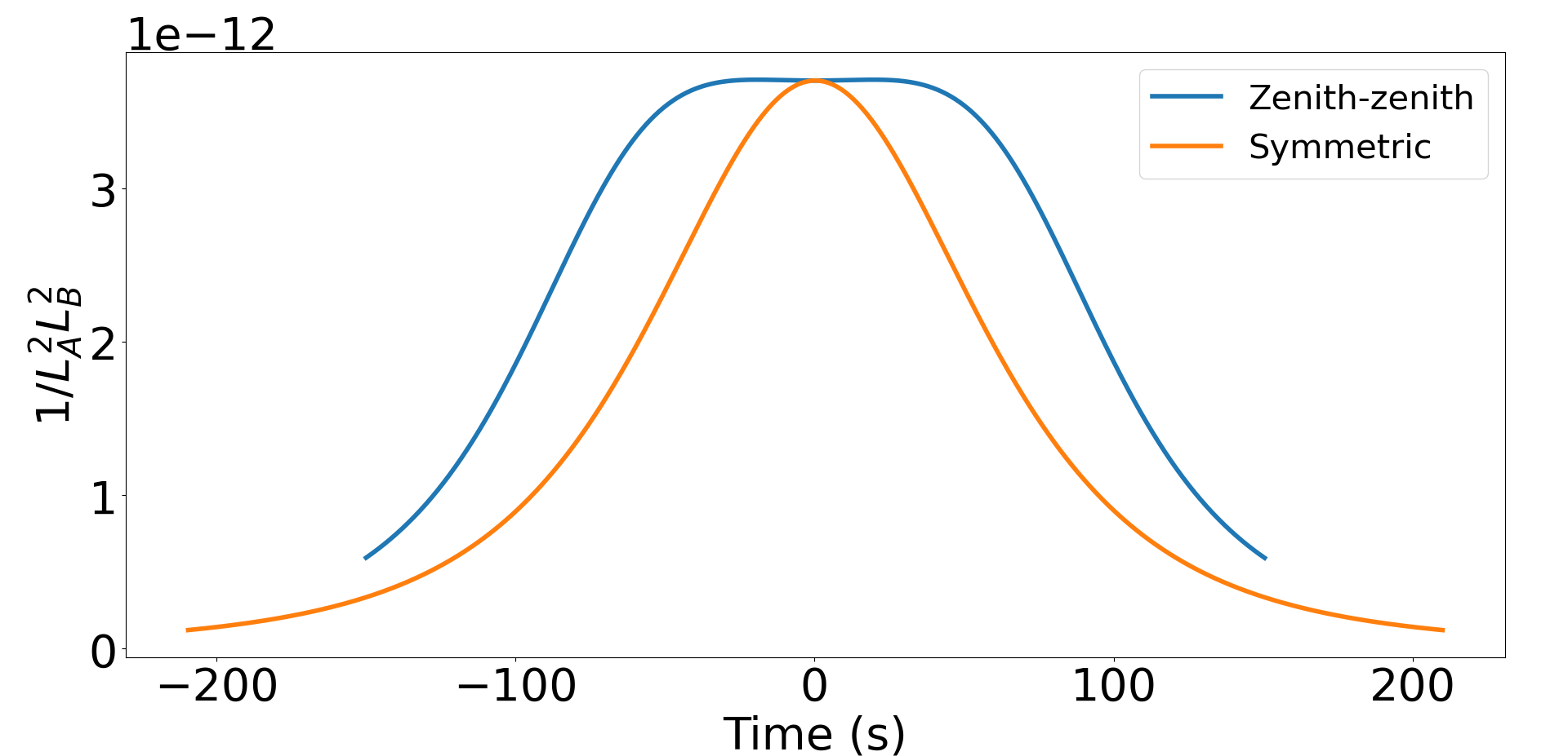
For the repeater satellite, the instantaneous PDR behaves as,(Eq. 2)

$$R^{\text{SSQR}}\sim\min\{1/L^{3}_{A},1/L^{3}_{B}\},$$ (C2)

due to channel loss $\sim\frac{1}{L_{A,B}^{2}}$ and the attempt rate $\sim\frac{1}{L_{A,B}}$. Fig. C1(b) illustrates this scaling for the zenith-zenith and symmetric overpasses. In this case the symmetric overpass yields a flatter rate distribution than zenith-zenith, with a corresponding higher per-overpass PDV after integration. The higher PDV in this case can also be seen directly from Eq. C2, where the rate is maximised when $L_{A}=L_{B}$, which is satisfied for all points in a symmetric overpass.

(a) DDDL scaling (Eq. C1)

(b) SSQR scaling (Eq. C2)

Figure C1: Scaling of the instantaneous pair distributions for the zenith-zenith and symmetric overpasses. The $t=0$ point here corresponds to where the satellite is equidistant from Alice and Bob ($\sim 720$km for $d=1000$km and $h=500$km). Since the per-overpass PDV is found by integrating the instantaneous pair distribution rates, a broader distribution leads to superior performance. Thus zenith-zenith is optimal for DDDL and symmetric is optimal for SSQR.

Appendix D Memory Noise Model

Here, we detailed our calculations for the fidelity of the pair that Alice and Bob having in hand after the satellite performs entanglement swapping. We assume that the satellite produces perfect entanglement pairs of fidelity $1$. Under this assumptions, the only fidelity losses in the system are due to memory imperfections. We denote the memory lifetimes $\tau_{\text{mem}}$, which is assumed to be equal across all memory slots on board the satellite. The pairs that the satellite generates on board of the form

$$\rho_{AS_{1}BS_{2}}=\ket{\Phi^{+}}\bra{\Phi^{+}}_{AS_{1}}\otimes\ket{\Phi^{+}}\bra{\Phi^{+}}_{BS_{2},}$$ (D1)

where A and Bob are Alice and Bob, respectively, and $S_{1}$, $S_{2}$ are internal states of the satellite memory. While the states are held in memory waiting for confirmation of successful transmission, they are subject to dephasing noise, a common model of memory noise that is present in the literature [38]. The qubit held in memory undergoes dephasing noise according to

$$D(t)\rho:\rho\mapsto(1-\lambda(t))\rho\otimes\lambda(t)Z\rho Z,$$ (D2)

where

$$\lambda(t)=\frac{1-\exp(-t/\tau_{\text{mem}})}{2},$$ (D3)

and $t$ is the time the qubit has been waiting in memory. In our model, it is only qubits on the satellite that are subject to dephasing noise. One can easily see that

$$(I\otimes D(t))\ket{\Phi^{+}}\bra{\Phi^{+}}=(1-\lambda(t))\ket{\Phi^{+}}\bra{\Phi^{+}}+\lambda(t)\ket{\Phi^{-}}\bra{\Phi^{-}}.$$ (D4)

The state of the two qubit pairs on-board the satellite just performed swapping is performed is given by

$$\rho_{AS_{1}BS_{2}}(t_{A},t_{B})=(I_{A}\otimes D(t_{A})_{S_{1}})\otimes(I_{B}\otimes D(t_{B})_{S_{2}})\rho_{AS_{1}BS_{2}},$$ (D5)

where $t_{A}$ and $t_{B}$ are the total times that each pair has been sitting in memory. The satellite then performs entanglement swapping on this pair, in order to establish direct entanglement between Alice and Bob. This consists of performing a Bell state measurement on the $S_{1}S_{2}$ pair, and classically communicating the results to the ground stations. One can show that under the above memory noise model, the state that the ground stations have in their possession is given by

$$\rho_{AB}= \left[\lambda\left(t_{A}\right)\lambda\left(t_{B}\right)+\left(1-\lambda\left(t_{A}\right)\right)\left(1-\lambda\left(t_{B}\right)\right)\right]\ket{\Phi^{+}}\bra{\Phi^{+}}$$ (D6)

$$+\left[\lambda\left(t_{A}\right)\left(1-\lambda\left(t_{B}\right)\right)+\lambda\left(t_{A}\right)(1-\lambda\left(t_{B}\right))\right]\ket{\Phi^{-}}\bra{\Phi^{-}}.$$ (D7)

The fidelity can be easily read off the above equation as coefficient in front of $\ket{\Phi^{+}}\bra{\Phi^{+}}$.

Appendix E Monte Carlo Methods

In Sec. 3.3 we employ a MC model to assess the waiting time statistics of memory qubits. This allowed us to evaluate the effects that a finite memory lifetime has on the fidelity of the distributed entanglement. In this section we provide some details on the MC methods. A list of variables used in the MC processes presented in Tab. 4

Variable	Description
$M_{A(B)}$	Arrays that track the state of the Alice (Bob) memory register: $0$ indicates no confirmation from OGS, $1$ indicates successful transmission confirmed.
$T_{A(B)}$	Arrays recording memory qubit loading times: updated upon confirmation of transmission, set to $0$ otherwise.
$W_{A(B)}$	Lists recording waiting time of Alice (Bob) memory qubits consumed in swapping operations, updated when qubit is swapped.
$\tau_{A(B)}$	One-way photon transit time to Alice (Bob).
$\eta_{A(B)}$	Alice (Bob) channel transmissivities.
$t_{0}$	Time at beginning of current time step.
$b$	Buffer size, memory registers are trimmed to this size before next entanglement generation attempt.
$N_{\text{SSQR}}$	Number of successfully swapped pairs in this time step, incremented when a qubit pairs is swapped.

Table 4: Description of key variables used in the MC process.

In the model the satellite is propagated in time steps of dt, with channel parameters updated at the beginning of each time step. Within each time step, starting at $t_{0}$, the process of SSQR entanglement distribution is simulated until a time $t_{0}+\text{dt}$ is reached. This involved updated the states of memories, recording storage times, and overall SSQR counts. The state of the memories at the end of one time step is used to initialise the next time step, until a full overpass has been simulated.

Pseudocode for the MC process within a time step is shown in Algor. 1. $N_{\text{SSQR}}$, $W_{A}$, $W_{B}$ and an internal time tracker are initialised. The satellite then repeats the process of performing entanglement swapping (Algor. 2), trimming the registers to the buffer size (Algor. 3) and attempting to generate entanglement (Algor. 4) with the OGSs until a time dt has elapsed. At the end of the time step the outputs $N_{\text{SSQR}}$, $W_{A}$ and $W_{B}$ are used to build the statistical sample that was used to produce the results in Sec 3.3.

We refer to the MC model as round-based in the main text because the memory and storage time arrays are updated only at times when classical signals arrive from the ground stations. This means that the $M_{A(B)}$, $T_{A(B)}$ arrays are updated in steps of $2\tau_{A(B)}$. It is this round-based approach that leads to the beats in the waiting times seen in the main text (e.g. Fig 16(a) at $t\sim-50s$. When

$$n\tau_{A}=m\tau_{B}$$ (E1)

is satisfied for $n,m\in\mathbb{Z}$ classical signals arrive from Alice and Bob arrive simultaneously. These qubits are available to use in swapping with the minimum possible waiting times (the round-trip time) which has the effect of reducing the median waiting time.

1

2SSQR_MonteCarlo$\big(M_{A},M_{B},T_{A},T_{B},\tau_{A},\tau_{B},\eta_{A},\eta_{B},t_{0},\text{b}\big)$

; Input : memory arrays, storage time arrays, photon transit times, channel transmissivities, start time and buffer size.

Output : updated memory arrays, updated time arrays, waiting times, SSQR counts, Alice counts, Bob counts, final time.

3 $N_{\text{SSQR}}\leftarrow 0$

4 $W_{A}\leftarrow[]$, $W_{B}\leftarrow[]$

5 $t_{\text{internal}}\leftarrow 0$

6 timeA $\leftarrow$ $2\tau_{A}$, timeB $\leftarrow 2\tau_{B}$

7 while $t_{\text{internal}}\leq$dt do

8    $M_{A}$, $M_{B}$, $T_{A}$,$T_{B}\leftarrow$entanglementSwapping($M_{A}$, $M_{B}$, $T_{A}$, $T_{B}$)

9    $M_{A}$, $T_{A}$ $\leftarrow$ TrimToBuffer($M_{A}$, $T_{A}$, b)

10    $M_{B}$, $T_{B}$ $\leftarrow$ TrimToBuffer($M_{B}$, $T_{B}$, b)

11    $M_{A},M_{B},T_{A},T_{B}\leftarrow$ EntanglementGeneration($M_{A},M_{B},T_{A},T_{B}$)

12 end while

return $M_{A},M_{B},T_{A},T_{B},W_{A},W_{B},N_{\text{SSQR}},N_{\text{Alice}},N_{\text{Bob}}$, $t_{0}+t_{\text{internal}}$

Algorithm 1 Pseudocode for the Monte Carlo process. The satellite performs the processed of entanglement swapping, trimming the registers to the buffer size and attempting to generate entanglement within the current time step. The $M_{A(B)}$ and $T_{A(B)}$ arrays are outputted to initialise the next time step. The waiting times lists $W_{A}(B)$ are recorded to built statistics for the full overpass.

1EntanglementSwapping$\big(M_{A},M_{B},T_{A},T_{B}\big)$

; Input : memory arrays, storage time arrays.

Output : updated memory arrays, storage time array.

2 GLOBAL $N_{\text{SSQR}}$, $W_{A},W_{B}$

3 while sum($M_{A}$) $>0$ AND sum($M_{B}$) $>0$ do

4    $N_{\text{SSQR}}$ += 1

5    readyAlice $\leftarrow$ [], readyBob $\leftarrow$ []

6    readyAliceTimes $\leftarrow[]$, readyBobTimes $\leftarrow[]$

7    for i in 1 to length($M_{B}$) do

8       if $M_{A}[i]>0$ then

9          append i to readyAlice

10          append $T_{A}$[i] to readyAliceTimes

11         

12       end if

13      

14    end for

15   for i in 1 to length($M_{B}$) do

16       if $M_{B}[i]>0$ then

17          append i to readyBob

18          append $T_{A}$[i] to readyBobTimes

19         

20       end if

21      

22    end for

   // choose youngest pairs to swap

23    aliceSlot $\leftarrow$ max(readyAliceTimes)

24    bobSlot $\leftarrow$ max(readyBobTimes)

25    append ($t_{0}+t_{\text{internal}}$ - $T_{A}$[aliceSlot]) to $W_{A}$

26    append ($t_{0}+t_{\text{internal}}$ - $T_{B}$[bobSlot]) to $W_{B}$

27    $M_{A}$[aliceSlot] $\leftarrow 0$, $T_{A}$[aliceSlot] $\leftarrow 0$

28    $M_{B}$[bobSlot] $\leftarrow 0$, $T_{B}$[bobSlot] $\leftarrow 0$

29   

30 end while

31

return $M_{A}$, $M_{B}$, $T_{A}$, $T_{B}$

Algorithm 2 Entanglement swapping. While there is one or more successfully transmitted qubits in each of the Alice and Bob registers the satellite performs swapping. $N_{\text{SSQR}}$ is incremented and the youngest pairs (picked by argmax) are chosen for swapping. The $M_{A(B)}$ and $T_{A(B)}$ arrays are updated to reflect the qubits being consumed.

1TrimToBuffer$\big(M,T,b\big)$

; Input : memory array, storage time array, buffer size.

Output : updated memory and storage time arrays

2 while $sum(M)>b$ do

3    listMems $\leftarrow$ []

4    timesList $\leftarrow$ []

5    for $i\leftarrow 1$ to $\text{length}(M)$ do

6       if $M[i]>0$ then

7          append i to listMems

8          append $T[i]$ to timesList

9         

10       end if

11      

12    end for

   // discard oldest pairs

13    $M[listMems[argmin(listTimes)]]\leftarrow 0$

14    $T[listMems[argmin(listTimes)]]\leftarrow 0$

15 end while

16

return M, T

Algorithm 3 Trim to buffer size. If the current number of held (successfully transmitted) pairs is greater than the buffer size then qubits are discarded until $b$ remain. The oldest pairs, chosen by argmin, are chosen for to be discarded.

1EntanglementGeneration$\big(M_{A},M_{B},T_{A},T_{B}\big)$

; Input : memory arrays, storage time arrays.

Output : updated memory and storage time arrays.

2 if $timeA=timeB$ then

3    event $\leftarrow[^{\prime}Alice^{\prime},^{\prime}Bob^{\prime}]$

4    $t_{\text{internal}}\leftarrow timeA$

5   

6 end if

7else if $timeA<timeB$ then

8    event $\leftarrow[^{\prime}Alice^{\prime}]$

9    $t_{\text{internal}}\leftarrow timeA$

10   

11 end if

12else if $timeB<timeA$ then

13    event $\leftarrow[^{\prime}Bob^{\prime}]$

14    $t_{\text{internal}}\leftarrow timeB$

15 end if

16for x in event do

17    if x = Alice then

18       sample $\leftarrow$ sampleBinomial(length($M_{A}$) - sum($M_{A}$), $\eta_{A}$)

19       if sample $>0$ then

20          slots $\leftarrow[]$

21          counter $\leftarrow$ 0

22          for i in 1 to length($M_{A}$) do

23             if $M_{A}[i]$ AND counter $<=$ sample then

24                append i to slots

25             end if

26            

27          end for

28         for i in 1 to sample do

29             $M_{A}[slots[i]\leftarrow 1$

30             $T_{A}[i]\leftarrow t_{0}+t_{\text{internal}}-2\tau_{A}$

31          end for

32         

33       end if

34      timeA += $2\tau_{A}$

35    end if

36   if x = Bob then

37       sample $\leftarrow$ sampleBinomial(length($M_{B}$) - sum($M_{B}$), $\eta_{B}$)

38       if sample $>0$ then

39          slots $\leftarrow[]$

40          counter $\leftarrow$ 0

41          for i in 1 to length($M_{B}$) do

42             if $M_{B}[i]>0$ AND counter $<=$ sample then

43                append i to slots

44               

45             end if

46            

47          end for

48         for i in 1 to sample do

49             $M_{B}[slots[i]\leftarrow 1$

50            

51          end for

52         for i in 1 to sample do

53             $M_{B}[slots[i]\leftarrow 1$

54             $T_{B}[i]\leftarrow t_{0}+t_{\text{internal}}-2\tau_{B}$

55            

56          end for

57         

58       end if

59      timeB += $2\tau_{B}$

60    end if

61   

62 end for

return $M_{A},M_{B},T_{A},T_{B}$

Algorithm 4 Entanglement generation algorithm. The OGS from which the next confirmation signal is expected is first identified. The number of successfully transmitted photons are then determined by sampling from a binomial distribution and the internal time is updated accordingly. The memory and loading time arrays are updated conditioned on successful transmission. with the $-2\tau$ terms (e.g. line 24) reflecting the fact that the qubits were transmitted at an earlier time.

References

- [1] Charles H. Bennett and Gilles Brassard. Quantum cryptography: Public key distribution and coin tossing. Theoretical Computer Science, 560:7–11, 2014.
- [2] Peter W. Shor and John Preskill. Simple proof of security of the bb84 quantum key distribution protocol. Physical Review Letters, 85(2):441–444, July 2000.
- [3] Valerio Scarani, Helle Bechmann-Pasquinucci, Nicolas J. Cerf, Miloslav Dušek, Norbert Lütkenhaus, and Momtchil Peev. The security of practical quantum key distribution. Reviews of Modern Physics, 81(3):1301–1350, September 2009.
- [4] Vittorio Giovannetti, Seth Lloyd, and Lorenzo Maccone. Quantum metrology. Physical review letters, 96(1):010401, 2006.
- [5] Christian L Degen, Friedemann Reinhard, and Paola Cappellaro. Quantum sensing. Reviews of modern physics, 89(3):035002, 2017.
- [6] Jianxin Shi and Shanshan Shen. A clock synchronization method based on quantum entanglement. Scientific Reports, 12:10185, 06 2022.
- [7] Peter W. Shor. Polynomial-time algorithms for prime factorization and discrete logarithms on a quantum computer. SIAM Journal on Computing, 26(5):1484–1509, October 1997.
- [8] S. Pirandola, U. L. Andersen, L. Banchi, M. Berta, D. Bunandar, R. Colbeck, D. Englund, T. Gehring, C. Lupo, C. Ottaviani, J. L. Pereira, M. Razavi, J. Shamsul Shaari, M. Tomamichel, V. C. Usenko, G. Vallone, P. Villoresi, and P. Wallden. Advances in quantum cryptography. Advances in Optics and Photonics, 12(4):1012, December 2020.
- [9] H.-J. Briegel, W. Dür, J. I. Cirac, and P. Zoller. Quantum repeaters: The role of imperfect local operations in quantum communication. Phys. Rev. Lett., 81:5932–5935, Dec 1998.
- [10] Chao-Yang Lu, Yuan Cao, Cheng-Zhi Peng, and Jian-Wei Pan. Micius quantum experiments in space. Rev. Mod. Phys., 94:035001, Jul 2022.
- [11] Jasminder S. Sidhu, Siddarth K. Joshi, Mustafa Gündoğan, Thomas Brougham, David Lowndes, Luca Mazzarella, Markus Krutzik, Sonali Mohapatra, Daniele Dequal, Giuseppe Vallone, Paolo Villoresi, Alexander Ling, Thomas Jennewein, Makan Mohageg, John G. Rarity, Ivette Fuentes, Stefano Pirandola, and Daniel K. L. Oi. Advances in space quantum communications. IET Quantum Communication, 2(4):182–217, July 2021.
- [12] Alessio Belenchia, Matteo Carlesso, Ömer Bayraktar, Daniele Dequal, Ivan Derkach, Giulio Gasbarri, Waldemar Herr, Ying Lia Li, Markus Rademacher, Jasminder Sidhu, et al. Quantum physics in space. Physics Reports, 951:1–70, 2022.
- [13] Seid Koudia, Junaid ur Rehman, and Symeon Chatzinotas. Space-based quantum internet: Entanglement distribution in time-varying leo constellations. arXiv:2409.17032, 2024.
- [14] Mustafa Gündogan, Jasminder S. Sidhu, Victoria Henderson, Luca Mazzarella, Janik Wolters, Daniel K. L. Oi, and Marcus Krutzik. Proposal for space-borne quantum memories for global quantum networking. npj Quantum Information, 7, August 2021.
- [15] Paolo Fittipaldi, Kentaro Teramoto, Naphan Benchasattabuse, Michal Hajdušek, Rodney Van Meter, and Frédéric Grosshans. Entanglement swapping in orbit: a satellite quantum link case study. In 2024 IEEE International Conference on Quantum Computing and Engineering (QCE), page 1924–1930. IEEE, September 2024.
- [16] Carlo Liorni, Hermann Kampermann, and Dagmar Bruß. Quantum repeaters in space. New Journal of Physics, 23(5):053021, May 2021.
- [17] Mustafa Gündoǧan, Jasminder S Sidhu, Markus Krutzik, and Daniel KL Oi. Time-delayed single satellite quantum repeater node for global quantum communications. Optica Quantum, 2(3):140–147, 2024.
- [18] Jasminder S Sidhu, Sarah E McCarthy, Cameron Paterson, and Daniel KL Oi. Operational limits to entanglement-based satellite quantum key distribution. arXiv preprint arXiv:2602.11833, 2026.
- [19] Jasminder S Sidhu, Thomas Brougham, Duncan McArthur, Roberto G Pousa, and Daniel KL Oi. Finite key effects in satellite quantum key distribution. npj Quantum Information, 8(1):18, 2022.
- [20] Tanvirul Islam, Jasminder S. Sidhu, Brendon L. Higgins, Thomas Brougham, Tom Vergoossen, Daniel K.L. Oi, Thomas Jennewein, and Alexander Ling. Finite-resource performance of small-satellite-based quantum-key-distribution missions. PRX Quantum, 5:030101, Jul 2024.
- [21] Cody Jones, Danny Kim, Matthew T Rakher, Paul G Kwiat, and Thaddeus D Ladd. Design and analysis of communication protocols for quantum repeater networks. New Journal of Physics, 18(8):083015, August 2016.
- [22] Koji Azuma, Kiyoshi Tamaki, and Hoi-Kwong Lo. All-photonic quantum repeaters. Nature communications, 6(1):6787, 2015.
- [23] Xingling Pan, Zhiming Chen, Yingtao Ding, Weibo Gao, Fei Ding, and Zhaogang Dong. Quantum dots as solid-state sources of entangled photon pairs. arXiv preprint arXiv:2602.05245, 2026.
- [24] Aitor Villar, Alexander Lohrmann, Xueliang Bai, Tom Vergoossen, Robert Bedington, Chithrabhanu Perumangatt, Huai Ying Lim, Tanvirul Islam, Ayesha Reezwana, Zhongkan Tang, et al. Entanglement demonstration on board a nano-satellite. Optica, 7(7):734–737, 2020.
- [25] Sarah E McCarthy, Ali Anwar, Daniel KL Oi, and Loyd J McKnight. Compact and stable source of polarization-entangled photon-pairs based on a folded linear displacement interferometer. Optics Express, 33(18):38657–38668, 2025.
- [26] Xingyu Wang, Jiahao Li, Bolong Wang, Yuexiang Cao, Yonghui Li, Haoran Hu, Qian Li, Nan Xiao, Chen Dong, Kai Guo, and Lei Shi. Scalability bottlenecks in entanglement-based satellite quantum key distribution: downlink asymmetry, orbit dependence and finite-key effects. preprint https://doi.org/10.21203/rs.3.rs-8708341/v1, 2026.
- [27] L-M Duan, Mikhail D Lukin, J Ignacio Cirac, and Peter Zoller. Long-distance quantum communication with atomic ensembles and linear optics. Nature, 414(6862):413–418, 2001.
- [28] Koji Azuma, Sophia E Economou, David Elkouss, Paul Hilaire, Liang Jiang, Hoi-Kwong Lo, and Ilan Tzitrin. Quantum repeaters: From quantum networks to the quantum internet. Reviews of Modern Physics, 95(4):045006, 2023.
- [29] William J. Munro, Koji Azuma, Kiyoshi Tamaki, and Kae Nemoto. Inside quantum repeaters. IEEE Journal of Selected Topics in Quantum Electronics, 21(3):78–90, 2015.
- [30] K Boone, J-P Bourgoin, E Meyer-Scott, K Heshami, T Jennewein, and C Simon. Entanglement over global distances via quantum repeaters with satellite links. Physical Review A, 91(5):052325, 2015.
- [31] Manik Dawar, Clement Paillet, Nilesh Vyas, Andrew Thain, Rodrigo Henriques Guilherme, and Ralf Riedinger. Feasibility of satellite-augmented global quantum repeater networks. arXiv preprint arXiv:2603.11127, 2026.
- [32] Matthias J. Bayerbach, Simone E. D’Aurelio, Peter van Loock, and Stefanie Barz. Bell-state measurement exceeding 50% success probability with linear optics. Science Advances, 9(32):eadf4080, 2023.
- [33] Luca Mazzarella, Christopher Lowe, David Lowndes, Siddarth Koduru Joshi, Steve Greenland, Doug McNeil, Cassandra Mercury, Malcolm Macdonald, John Rarity, and Daniel Kuan Li Oi. Quarc: Quantum research cubesat—a constellation for quantum communication. Cryptography, 4(1):7, 2020.
- [34] Martin B. Plenio and Shashank Virmani. An introduction to entanglement measures. Quantum Info. Comput., 7(1):1–51, January 2007.
- [35] Ryszard Horodecki, Paweł Horodecki, Michał Horodecki, and Karol Horodecki. Quantum entanglement. Reviews of Modern Physics, 81(2):865–942, June 2009.
- [36] Michał Horodecki, Paweł Horodecki, and Ryszard Horodecki. General teleportation channel, singlet fraction, and quasidistillation. Phys. Rev. A, 60:1888–1898, Sep 1999.
- [37] Laurent de Forges de Parny, Olivier Alibart, Julien Debaud, Sacha Gressani, Alek Lagarrigue, Anthony Martin, Alexandre Metrat, Matteo Schiavon, Tess Troisi, Eleni Diamanti, et al. Satellite-based quantum information networks: use cases, architecture, and roadmap. Communications Physics, 6(1):12, 2023.
- [38] Julius Wallnöfer, Frederik Hahn, Mustafa Gündoğan, Jasminder S Sidhu, Fabian Wiesner, Nathan Walk, Jens Eisert, and Janik Wolters. Simulating quantum repeater strategies for multiple satellites. Communications Physics, 5(1):169, 2022.
- [39] Mustafa Gündoğan, Patrick M. Ledingham, Kutlu Kutluer, Margherita Mazzera, and Hugues de Riedmatten. Solid state spin-wave quantum memory for time-bin qubits. Phys. Rev. Lett., 114:230501, Jun 2015.
- [40] Bo Zhao, Yu-Ao Chen, Xiao-Hui Bao, Thorsten Strassel, Chih-Sung Chuu, Xian-Min Jin, Jörg Schmiedmayer, Zhen-Sheng Yuan, Shuai Chen, and Jian-Wei Pan. A millisecond quantum memory for scalable quantum networks. Nature Physics, 5(2):95–99, 2009.
- [41] Manjin Zhong, Morgan P Hedges, Rose L Ahlefeldt, John G Bartholomew, Sarah E Beavan, Sven M Wittig, Jevon J Longdell, and Matthew J Sellars. Optically addressable nuclear spins in a solid with a six-hour coherence time. Nature, 517(7533):177–180, 2015.
- [42] Pierre Jobez, Nuala Timoney, Cyril Laplane, Jean Etesse, Alban Ferrier, Philippe Goldner, Nicolas Gisin, and Mikael Afzelius. Towards highly multimode optical quantum memory for quantum repeaters. Phys. Rev. A, 93:032327, Mar 2016.
- [43] Nasser Gohari Kamel, Arsalan Mansourzadeh, Ujjwal Gautam, Vinaya Kumar Kavatamane, Ashutosh Singh, Edith Yeung, David B Northeast, Paul Barclay, Philip J Poole, Dan Dalacu, et al. Erbium-doped fibre quantum memory for chip-integrated quantum-dot single photons at 980 nm. arXiv preprint arXiv:2508.01416, 2025.
- [44] Shi-Hai Wei, Bo Jing, Xue-Ying Zhang, Jin-Yu Liao, Hao Li, Li-Xing You, Zhen Wang, You Wang, Guang-Wei Deng, Hai-Zhi Song, et al. Quantum storage of 1650 modes of single photons at telecom wavelength. npj Quantum Information, 10(1):19, 2024.
- [45] Julius Wallnöfer, Frederik Hahn, Fabian Wiesner, Nathan Walk, and Jens Eisert. Faithfully simulating near-term quantum repeaters. PRX Quantum, 5(1), March 2024.
- [46] Daoheng Niu, Yuxuan Zhang, Alireza Shabani, and Hassan Shapourian. All-photonic one-way quantum repeaters with measurement-based error correction. npj Quantum Information, 9(1):106, 2023.
- [47] Álvaro G Iñesta, Gayane Vardoyan, Lara Scavuzzo, and Stephanie Wehner. Optimal entanglement distribution policies in homogeneous repeater chains with cutoffs. npj Quantum Information, 9(1):46, 2023.
- [48] F Rozpȩdek, K Goodenough, J Ribeiro, N Kalb, V Caprara Vivoli, A Reiserer, R Hanson, S Wehner, and D Elkouss. Parameter regimes for a single sequential quantum repeater. Quantum Science and Technology, 3(3):034002, apr 2018.
- [49] J Yin, Y-H Li, S-K Liao, M Yang, Y Cao, L Zhang, J-G Ren, W-Q Cai, W-Y Liu, S-L Li, R Shu, Y-M Huang, L Deng, L Li, Q Zhang, N-L Liu, Y-A Chen, C-Y Lu, X-B Wang, F Xu, X-B Wang, C-Z Peng, AK Ekert, and J-W Pan. Entanglement-based secure quantum cryptography over 1,120 kilometres. Nature, 582:501–505, 2020.
- [50] Jaya Sagar, Elliott Hastings, Peide Zhang, Milan Stefko, David Lowndes, Daniel Oi, John Rarity, and Siddarth K Joshi. Design and test of optical payload for polarization encoded qkd for nanosatellites. In Quantum Technology: Driving Commercialisation of an Enabling Science III, volume 12335, pages 64–70. SPIE, 2023.
- [51] Daniel KL Oi, Alex Ling, Giuseppe Vallone, Paolo Villoresi, Steve Greenland, Emma Kerr, Malcolm Macdonald, Harald Weinfurter, Hans Kuiper, Edoardo Charbon, and Rupert Ursin. Cubesat quantum communications mission. EPJ Quantum Technology, 4(1), April 2017.
- [52] Sumit Goswami, Sayandip Dhara, Neil Sinclair, Makan Mohageg, Jasminder S Sidhu, Sabyasachi Mukhopadhyay, Markus Krutzik, John R Lowell, Daniel KL Oi, Mustafa Gündoğan, et al. Satellites promise global-scale quantum networks. Optica Quantum, 3(6):590–605, 2025.
- [53] Ali Anwar, Chithrabhanu Perumangatt, Fabian Steinlechner, Thomas Jennewein, and Alexander Ling. Entangled photon-pair sources based on three-wave mixing in bulk crystals. Review of Scientific Instruments, 92(4), 2021.
- [54] Poramet Pathumsoot, Theerapat Tansuwannont, Naphan Benchasattabuse, Ryosuke Satoh, Michal Hajdušek, Poompong Chaiwongkhot, Sujin Suwanna, and Rodney Van Meter. Boosting end-to-end entanglement fidelity in quantum repeater networks via hybridized strategies. In 2024 International Conference on Quantum Communications, Networking, and Computing (QCNC), pages 49–56. IEEE, 2024.
- [55] Jean-Philippe Bourgoin, Evan Meyer-Scott, Brendon L Higgins, B Helou, Chris Erven, Hannes Huebel, B Kumar, D Hudson, Ian D’Souza, Ralph Girard, et al. A comprehensive design and performance analysis of low earth orbit satellite quantum communication. New Journal of Physics, 15(2):023006, 2013.
- [56] A. Berk, P. Conforti, R. Kennett, T. Perkins, F. Hawes, and J. van den Bosch. Modtran® 6: A major upgrade of the modtran® radiative transfer code. In 2014 6th Workshop on Hyperspectral Image and Signal Processing: Evolution in Remote Sensing (WHISPERS), pages 1–4, 2014.