DeferredSeg: A Multi-Expert Deferral Framework for Trustworthy Medical Image Segmentation

Abstract

Segmentation models based on deep neural networks demonstrate strong generalization for medical image segmentation. However, they often exhibit overconfidence or underconfidence, leading to unreliable confidence scores for segmentation masks, especially in ambiguous regions. This undermines the trustworthiness required for clinical deployment. Motivated by the learning-to-defer (L2D) paradigm, we introduce DeferredSeg, a deferral-aware segmentation framework, i.e., a Human–AI collaboration system that determines whether to defer predictions to human experts in specific regions.

DeferredSeg extends the base segmentor with an aggregated deferral predictor and additional routing channels that dynamically route each pixel to either the base segmentor or a human expert. To train this routing efficiently, we introduce a pixel-wise surrogate collaboration loss that supervises deferral decisions. In addition, to preserve spatial coherence within deferral regions, we propose a spatial-coherence loss that enforces smooth deferral masks, thereby enhancing reliability.

Beyond single-expert deferral, we further extend the framework to a multi-expert setting by introducing multiple discrepancy experts for collaborative decision-making. To prevent overloading or underutilizing individual experts, we further design a load-balancing penalty that evenly distributes workload across expert branches. We evaluate DeferredSeg on three challenging medical datasets using MedSAM and CENet as the base segmentor for fair comparison. Experimental results show that DeferredSeg consistently outperforms the baseline, demonstrating its effectiveness for trustworthy dense medical segmentation. Moreover, the proposed framework is model-agnostic and can be readily applied to other segmentation architectures.

[inst1] organization=School of Software, Shandong University, city=Jinan, postcode=250101, country=China

[inst2] organization=Department of Clinical Laboratory, Shandong Provincial Hospital Affiliated to Shandong First Medical University, city=Jinan, postcode=250021, country=China

[inst3] organization=School of Computer Science and Technology, Nanjing University, city=Nanjing, postcode=210023, country=China

1 Introduction

Medical image segmentation is a fundamental task in medical data analysis, aiming to assign a semantic label to every pixel or voxel in an image. Accurate delineation of anatomical structures or pathological regions is crucial for a broad range of downstream applications, including computer-aided diagnosis, treatment planning, and intraoperative navigation [25, 51]. Compared to natural image segmentation, medical segmentation is inherently more challenging due to heterogeneous imaging modalities, low-contrast boundaries, irregular shapes, and the scarcity of high-quality annotations [6]. Traditional approaches such as graph-based [46] and energy-based [5] methods have demonstrated effectiveness, but deep neural networks now dominate medical image segmentation. Skip-connection architectures, notably U-Net [44] and its variants [42, 37, 20], remain strong clinical baselines. Recent Transformer-based designs, including H2Former [14], UNETR [13], and Swin-UNet [4], further enhance performance by modeling long-range dependencies. Although these models have demonstrated remarkable generalization ability, recent studies report that these deep models often produce overconfident or underconfident predictions [23, 24]. This tendency is particularly evident in ambiguous or low-contrast regions, such as fuzzy boundaries, small lesions, and distribution shifts [36]. In high-stakes medical segmentation, such issues pose a critical risk: incorrect predictions delivered with high certainty may mislead clinicians and cause severe consequences.

Therefore, relying solely on automated outputs is unsafe; incorporating Human–AI collaboration that integrates clinical expertise into the decision-making process for high-risk cases is essential. Several interactive segmentation methods have been proposed, such as MIDeepSeg [31] and TIS [28], which reduce the amount of user interaction required. However, these methods still require the user to make decisions on the entire image, rather than focusing on smaller, more ambiguous regions.

The learning-to-defer paradigm addresses this issue by allowing a model to either make its own prediction or defer to an expert when confidence is low [33, 38, 49, 52]. Unlike conventional uncertainty-estimation approaches, which are typically used only for post-hoc calibration or as auxiliary training signals [39, 12], L2D treats uncertainty as an explicit, actionable decision variable, enabling dynamic, task-adaptive routing to experts. Recent studies have demonstrated the effectiveness of L2D in classification tasks [10] and explored its role in safety-critical domains such as medical decision-making [48] and content moderation systems [41]. However, existing L2D methods operate at the instance level, making them unsuitable for dense prediction tasks where uncertainty varies spatially at the pixel level. In medical segmentation, such instance-wise deferral cannot resolve localized ambiguities, including unclear tissue boundaries and heterogeneous lesion textures. This motivates a region-selective collaboration strategy for dense prediction, where only ambiguous regions are referred for expert review instead of requiring full-image correction.

Figure 1: Overview of DeferredSeg. A deferral predictor produces a pixel-wise deferral map that triages image regions between a human expert and the base segmentation model, enabling spatially adaptive Human–AI collaboration for reliable medical segmentation.

In this paper, we propose the first pixel-wise deferral-aware segmentation framework, named DeferredSeg, for trustworthy dense medical image segmentation. The core of our framework is a Human-AI collaboration system featuring a novel deferral predictor and a deferral function. These components dynamically route pixel-wise predictions, determining whether to accept the base segmentation model’s prediction or to defer ambiguous regions to a human expert for review, as illustrated in Fig. 1. To achieve this, we introduce several key innovations. For efficient training, we design a pixel-wise deferral collaboration loss to support deferral decisions while accounting for expert errors. To ensure the deferred regions are contiguous and interpretable, we propose a spatial-coherence loss that promotes spatially smooth deferral masks [30], enhancing reliability.

Furthermore, to prevent any single expert from being overloaded or underutilized, we introduce a load-balancing penalty that evenly distributes the workload. DeferredSeg is designed as a plug-and-play framework that can be incorporated into most modern segmentation models. We evaluate our method on diverse public benchmarks, demonstrating consistent improvements over a strong MedSAM baseline, particularly in challenging anatomical regions.

Our main contributions are:

1. A Novel Deferral-Aware Segmentation Framework. We introduce DeferredSeg, the first framework for Human-AI collaboration in segmentation. It features a dynamic deferral predictor that intelligently routes pixel-wise decisions to either the base model or a human expert. This is enabled by two tailored loss functions: a surrogate deferral collaboration loss for efficient training and a spatial-coherence loss to ensure deferred regions are spatially coherent and reliable.

2. A Multi-Expert Setting for Balanced Collaboration. Our method introduces multiple experts to facilitate collaborative decision-making. This includes a load-balancing penalty to distribute workload evenly across different expert branches, preventing overload or underutilization.

3. Seamless Integration with State-of-the-Art Models. We demonstrate the practicality of DeferredSeg by integrating it with the MedSAM model. Our approach adapts the model’s Transformer features and decoder outputs to add a collaborative decision-making capability without compromising its powerful generalization performance.

4. Comprehensive Evaluation and Superior Performance. We conduct extensive experiments on three challenging medical datasets, benchmarking against strong baselines like nnU-Net v2 and CENet. Our results show that DeferredSeg consistently achieves superior performance and produces more trustworthy segmentation, with significant gains in ambiguous regions.

2 Related Work

2.1 Image Segmentation

2.1.1 Classical Methods

Early medical image segmentation primarily relied on handcrafted algorithms such as energy-based models [5],threshold-based methods [45],and graph-based methods [46]. Although they performed well on high-contrast structures with clear boundaries, their reliance on low-level image cues made them highly sensitive to noise, imaging artifacts, and parameter tuning. Moreover, they often required extensive user interaction for initialization (e.g., seed points, contour placement) and lacked robustness when faced with anatomical variability, heterogeneous textures, or overlapping intensity distributions. Another inherent limitation was the poor scalability of handcrafted approaches: adapting them to new organs, modalities, or disease types usually demanded significant redesign of feature extractors or segmentation rules. As datasets grew in size and diversity, these methods were progressively replaced by data-driven learning approaches that automatically learn hierarchical representations from raw images [54].

2.1.2 Deep Learning Architectures

Building on the limitations of classical methods, learning-based approaches—particularly convolutional neural networks (CNNs)—have enabled data-driven solutions for segmentation [29]. Representative architectures include U-Net [44], which introduced an encoder–decoder design with skip connections and demonstrated effectiveness even with limited training data; V-Net [37], which extended encoder–decoder structures to volumetric 3D segmentation; and DeepMedic [20], which utilized multi-scale 3D CNNs with patch-based training. The nnU-Net framework [16] further standardized segmentation by providing a self-configuring pipeline that automates preprocessing, architecture selection, and training. Subsequent variants such as U-Net++ [55] and Attention U-Net [42] introduced nested architectures and attention mechanisms to refine boundary delineation. More recently, Transformer-based models have been explored within this paradigm. For example, MISSFormer [15] redesigns Transformer blocks to mix global attention with local context; Swin-UNet [4] replaces convolutional layers with Swin Transformer layers; and UNETR [13] employs a Transformer encoder with a U-Net decoder for 3D volumes. Although these models have improved segmentation performance, they continue to face challenges in handling low-contrast tissues, irregular boundaries, and rare anatomical structures, and they often require large curated datasets to achieve robust generalization [25]. In the context of interactive segmentation, several methods have been proposed, such as MIDeepSeg [31], which leverages user-provided clicks to refine segmentation and generalizes well to previously unseen objects, and TIS [28], which uses user clicks or annotations. However, despite reducing user interaction, these methods still require experts to make decisions across the entire image. Similarly, Patch-based Error Correction [22] focuses on correcting high-uncertainty regions through manual review. While this approach reduces manual review time by selecting patches that require attention, it still necessitates expert intervention for the selected regions.

2.1.3 Foundation Models for Image Segmentation

Foundation models have recently attracted increasing attention in image segmentation due to their strong generalization capabilities. They also promise zero-shot or few-shot performance across diverse modalities and anatomical structures in medical image segmentation. Among them, the Segment Anything Model (SAM) [21] is a large-scale segmentation framework trained on over 11 million images and 1 billion masks. It leverages spatial prompts—such as points, bounding boxes, and prior masks—to guide segmentation outputs, enabling flexible, prompt-based mask generation suitable for interactive and open-vocabulary settings. Unlike vision–language models such as CLIP [43] and ALIGN [19], which learn transferable visual representations from image–text pairs, SAM is optimized directly for segmentation via prompt-conditioned supervision. Inspired by SAM’s success in natural image segmentation, several works have adapted this paradigm to the medical domain. MedSAM [32] fine-tunes SAM on a large corpus of medical images, while preserving its prompt-based architecture, thereby establishing a strong baseline for generalizable segmentation. MA-SAM [53] further enhances spine segmentation through multi-atlas–guided pseudo-mask prompts and SAM adaptation with lightweight adapters. SAM-Adapter [7] introduces a plug-and-play approach by adding lightweight, domain-specific adapters to SAM’s backbone, improving performance in underrepresented modalities without retraining the full model. Despite these advances, prompt-based foundation models still face challenges in clinically critical scenarios, such as low-contrast regions, irregular boundaries, small lesions, and ambiguous structures, where precise delineation is essential for downstream decision-making.

2.2 Learning to Defer

L2D integrates algorithmic or human expertise into automated decision systems by learning a deferral policy: for each input, the system either issues an automated prediction or routes the example to one or more experts based on a learned deferral score that balances model risk and expert competence. This extends the classic learning to reject [1] by introducing a learned triage policy that weighs model confidence against expert competence [33, 41, 9, 10], making it particularly relevant to high-stakes domains such as healthcare [11], content moderation [41]. Direct optimization of the discontinuous deferral objective is intractable, so L2D research has focused on designing consistent, differentiable surrogates. A cost-sensitive, consistent surrogate loss using a softmax-based formulation was first proposed in [38]. A calibrated one-vs-all objective was introduced in [50], and underfitting in consistent loss optimization was addressed in [27]. For multi-expert scenarios, a consistent and calibrated surrogate was developed in [49], and a two-stage approach with a matching consistent loss was proposed in [34]. Other works have considered constraints such as sparse expert availability and probabilistic workload allocation [40]. The L2D framework has been extended beyond classification, including regression with expert deferral [35], sequential decision-making in healthcare [48], reinforcement learning with human-in-the-loop triage [47], and semi-supervised learning [40]. These demonstrate the generality of L2D as a mechanism for Human–AI collaboration across tasks and modalities.

2.3 Gap and Our Positioning

Most existing L2D approaches make routing decisions at the instance level, which is appropriate for classification or detection but ill-suited to dense segmentation where uncertainty varies spatially and errors concentrate along fine anatomical boundaries (e.g., fuzzy borders, low-contrast tissues, small lesions). To address this gap, we propose DeferredSeg, the first framework to bring pixel-wise learning-to-defer to dense medical image segmentation. At its core, DeferredSeg applies pixel-wise learning-to-defer: an L2D mechanism estimates deferral scores per pixel and performs learned routing to either the automated model or specialized expert branches.

3 Preliminaries

We begin by formalizing the general learning-to-defer problem with multiple experts, and then provide the formulation of the true risk for the 0–1 loss and its surrogates for optimization.

3.1 Data and Model

Suppose there are $J$ human experts involved in L2D tasks. For a $K$-class classification problem, each training example in L2D is represented as a triplet $(\mathbf{x},y,\mathbf{m})\sim\mathcal{D}$, where $\mathbf{x}\in\mathcal{X}$ is the input, $y\in\{1,\dots,K\}$ is the ground-truth label, and $\mathbf{m}\in\mathbb{R}^{J}$ is the vector of expert predictions with element $\mathbf{m}_{i}\in\{1,\dots,K\}$. In addition to a classifier $h:\mathcal{X}\rightarrow\mathbb{R}$, a deferral function $r:\mathcal{X}\rightarrow\{0,1,\dots,J\}$ determines whether to defer and, if so, to which expert. Specifically, when $r(\mathbf{x})=0$, the classifier makes the prediction; when $r(\mathbf{x})=j$, the classifier abstains and defers the decision to the $j$-th expert.

3.2 The True Risk of the 0–1 Loss

The true risk $\mathcal{L}$ of L2D is extended from a generalization of learning with rejection, as proposed in [8], which can be formalized as a 0–1 loss as follows:

$$\mathcal{L}_{0-1}(h,r)=\mathop{\mathbb{E}}\limits_{\mathbf{x},y,\mathbf{m}}\!\Big[\mathop{\mathbb{I}}\limits_{r(\mathbf{x})=0}~\mathop{\mathbb{I}}\limits_{h(\mathbf{x})\neq y}\;+\;\sum_{j=1}^{J}\mathop{\mathbb{I}}\limits_{r(\mathbf{x})=j}~\mathop{\mathbb{I}}\limits_{\mathbf{m}_{j}\neq y}\Big].$$ (1)

The estimated classifier and deferring function pair $(\hat{h},\hat{r})$ can be obtained by minimizing Eq. (1) on the training set $\mathcal{D}$. However, since $\mathcal{L}_{0\text{-}1}$ is discontinuous and non-convex, making direct minimization is impractical; we therefore adopt differentiable and consistent surrogates are adopted for optimization.

3.3 The Softmax-Based (SM) Surrogate Loss

The softmax-based loss is commonly used in L2D. We augment the label space as $\mathcal{Y}^{\perp}=\mathcal{Y}\cup\{\perp_{1},\dots,\perp_{J}\}$, where $\perp_{j}$ represents the option to defer to the $j$-th expert. We build a predictor $f:\mathcal{X}\rightarrow\mathbb{R}^{K+J}$, composed of the classifier $h$ and deferral function $r$. $f$ can also be decomposed into $K+J$ functions: $f_{k}:\mathcal{X}\rightarrow\mathbb{R}$ for $k\in\{1,\dots,K\}$, and $f_{\perp,j}:\mathcal{X}\rightarrow\mathbb{R}$ for $j\in\{1,\dots,J\}$, where $k,j$ denote the class and expert indexes, respectively. These $K+J$ functions are combined using a softmax-parameterized surrogate loss:

$$\mathcal{L}_{SM}^{J} (f_{1},\dots,f_{K},f_{\perp,1},\dots,f_{\perp,J};\mathbf{x},y,\mathbf{m})=$$

$$-\sum_{j=1}^{J}\mathbb{I}[\mathbf{m}_{j}=y]\log\left(\frac{\exp f_{\perp,j}(\mathbf{x})}{\sum_{y^{\prime}\in\mathcal{Y}^{\perp}}\exp f_{y^{\prime}}(\mathbf{x})}\right)-\log\left(\frac{\exp f_{y}(\mathbf{x})}{\sum_{y^{\prime}\in\mathcal{Y}^{\perp}}\exp f_{y^{\prime}}(\mathbf{x})}\right).$$ (2)

The first term maximizes the deferral function $f_{\perp,j}$ if the $j$-th expert’s prediction is correct. The second term ensures that the function $f_{k}$ is maximized for the true label. At test time the classifier prediction is obtained by selecting the largest score among the first $K$ outputs, and deferral is decided as follows:

$$r(\mathbf{x})=\begin{cases}0,&\text{if }f_{h}(\mathbf{x})>\max_{j\in\{1,\dots,J\}}f_{\perp,j}(\mathbf{x}),\\ \arg\max_{j\in\{1,\dots,J\}}f_{\perp,j}(\mathbf{x}),&\text{otherwise.}\end{cases}$$ (3)

4 Method

Our methodology builds on the L2D paradigm and extends it to the pixel level for dense medical image segmentation. We present DeferredSeg, a framework that introduces pixel-wise routing with multiple experts via an output-channel extension, enabling fine-grained deferral decisions across spatial regions. To train the model effectively, we design several key components: a pixel-wise surrogate collaboration loss to guide joint learning between the segmentor and experts, a spatial-coherence loss to encourage smooth and reliable deferral maps, and a load-balancing penalty to ensure fair utilization of multiple experts. These components are integrated into a unified optimization framework. Finally, we incorporate DeferredSeg into the MedSAM architecture to leverage strong pretrained representations while enabling deferral-aware medical segmentation.

4.1 Overall Framework

DeferredSeg is a pixel-wise deferral framework with multi-expert collaboration, designed to work with any base segmentation model. We augment the model’s output channels by adding multiple routing channels, where one corresponds to the base model and the remaining correspond to specialized expert branches. Additionally, we introduce a aggregated deferral predictor module, which is added to the base model to estimate pixel-wise deferral scores, thereby guiding the routing decisions.

Unlike traditional segmentation pipelines that assign each pixel to a single output, our framework dynamically routes pixel-wise predictions to either the primary model or one of the domain-specialized experts based on learned deferral scores. This confidence-driven routing enables adaptive segmentation by referring ambiguous or difficult pixels for expert review. By referring only selected regions rather than the full image, the framework is intended to concentrate expert effort on difficult areas and reduce unnecessary review on easier regions.

The system operates as follows. First, the input image is processed by the base segmentor to produce intermediate representations. These intermediate representations are fed into the aggregated deferral predictor and deferral function, which together estimate pixel-wise deferral scores. Using the deferral scores, each pixel is dynamically routed to either the base model or one of the expert branches. The final segmentation mask is generated by combining the outputs from all branches. This workflow allows DeferredSeg to leverage the generalization ability of the base segmentor while adaptively delegating uncertain or challenging pixels to specialized experts.

4.2 Pixel-Wise L2D with Multiple Experts

We describe a general case of pixel-wise dense segmentation with multiple experts. The goal is to enable each pixel to be routed either to the base segmentor or to one of the experts based on learned deferral scores.

4.2.1 Output Channel Extension and Pixel-wise Routing

Let $\mathbf{x}\in\mathcal{X}$ be an image of size $H\times W$, and let $i\in\{1,\dots,HW\}$ index pixels; $\mathbf{x}^{i}$ denotes the value at the $i$-th pixel. The ground-truth label of $\mathbf{x}^{i}$ is $y^{i}\in\{0,1\}$ for a binary segmentation task. To enable pixel-wise L2D with $J$ experts, we extend the base segmentor by adding $J{+}1$ routing channels. The original segmentation output channels remain unchanged. Therefore, the label space is defined $\mathcal{Y}^{\perp}=\mathcal{Y}\cup\{\perp_{0},\perp_{1},\cdots,\perp_{J}\}$, where the labels from $\perp_{0}$ to $\perp_{J}$ correspond to the additional routing channels. Unlike the classification setting in Sec. 3, in our segmentation setting, the predictor is composed of the base segmentor $f_{\text{seg}}:\mathcal{X}\to\mathbb{R}^{H\times W}$ and the deferral function $f_{\perp}:\mathcal{X}\to\mathbb{R}^{(J+1)\times H\times W}$. In practice, the base segmentor produces a probability prediction $\hat{y}^{i}\in[0,1]$ for the foreground class at each pixel $\mathbf{x}^{i}$. The deferral function outputs per-pixel logits $f_{\perp,j}(\mathbf{x}^{i})$ with $j\in\{0,\dots,J\}$. A larger $f_{\perp,0}(\mathbf{x}^{i})$ indicates a stronger preference to route pixel $i$ to channel $0$ (the base segmentor), while a larger $f_{\perp,j}(\mathbf{x}^{i})$ ($j>0$) indicates a stronger preference to route it to channel $j$ (the $j$-th expert). For the $j$-th expert branch, $\mathbf{m}_{j}^{i}\in\{0,1\}$ denotes the $j$-th expert’s binarized prediction at pixel $\mathbf{x}^{i}$.

4.2.2 The Deferral Collaboration Loss

To enable pixel-wise L2D, we adapt the softmax surrogate introduced in Sec. 3 (Eq. (3.3)) and generalize it as the Deferral Collaboration (DC) Loss for dense segmentation, which is defined as:

$$\mathcal{L}_{\text{DC}} (f_{seg},f_{\perp,0},\dots,f_{\perp,J};\mathbf{x}^{i},y^{i},\mathbf{m}^{i})=\frac{1}{HW}\sum_{i=1}^{HW}\Big[\sum_{j=1}^{J}\big(1-2\,\mathbb{I}[\mathbf{m}_{j}^{i}=y^{i}]\big)\log\left(\frac{\exp f_{\perp,j}(\mathbf{x}^{i})}{\sum_{t=0}^{J}\exp f_{\perp,t}(\mathbf{x}^{i})}\right)$$

$$-\mathbb{I}[\tilde{y}^{i}=y^{i}]\log\left(\frac{\exp f_{\perp,0}(\mathbf{x}^{i})}{\sum_{t=0}^{J}\exp f_{\perp,t}(\mathbf{x}^{i})}\right)-\Big(y^{i}\log\hat{y}^{i}+\big(1-y^{i}\big)\log\big(1-\hat{y}^{i}\big)\Big)\Big],$$ (4)

where $\mathbb{I}[\cdot]$ denotes the indicator function, $\tilde{y}^{i}=\mathbb{I}[\hat{y}^{i}\geq 0.5]$ denotes binarized segmentor prediction. Specifically:

• The first term increases the routing score $f_{\perp,j}(\mathbf{x}^{i})$ when the $j$-th expert binarized prediction matches the ground truth, and suppresses it otherwise.

• The second term maximizes the segmentor branch deferral score $f_{\perp,0}(\mathbf{x}^{i})$ if the segmentor prediction $\tilde{y}^{i}$ matches the ground truth.

• The third term is the pixel-wise binary cross-entropy (BCE) on the segmentor output $\hat{y}^{i}$, which supervises the foreground prediction itself.

The loss encourages each pixel to select the branch with the more reliable prediction. The thresholded prediction $\tilde{y}^{i}$ is used only to construct routing supervision, whereas the segmentation branch itself is optimized through the soft probability $\hat{y}^{i}$ in the BCE term.

During inference, the routing probability map $\mathcal{M}$ of the $j$-th expert at pixel $i$ is defined as:

$$\mathcal{M}_{j}^{\,i}\;=\;\frac{\exp\!\big(f_{\perp,j}(\mathbf{x}^{i})\big)}{\sum_{j=0}^{J}\exp\!\big(f_{\perp,j}(\mathbf{x}^{i})\big)}.$$ (5)

At test time, the deferral decision is made by comparing the routing logits, e.g., a pixel is assigned to the base segmentor if $f_{\perp,0}(\mathbf{x}^{i})$ is the largest among all $f_{\perp,j}(\mathbf{x}^{i})$.

4.2.3 Spatial-Coherence Loss

To generate a smooth deferral map and ensure that deferred regions are spatially coherent and reliable, we introduce an additional aggregated deferral predictor built with two convolutional layers and enforce consistency between its predictions and those of the deferral function score $f_{\perp,j}(\cdot)$ using a spatial coherence (SC) loss.

Motivation.: State-of-the-art medical image segmentation models often employ Vision Transformer (ViT)-based decoders. However, these architectures can be less effective for data-efficient deferral learning on small datasets, as ViTs exhibit weak inductive bias for spatial relevance due to their emphasis on long-range interactions [30]. To address this, we introduce a CNN-based predictor to complement the ViT by providing intra-patch locality, enabling the capture of fine structures within patches and improving the spatial smoothness of deferral maps.

Let $\tilde{\mathcal{M}}\in\mathbb{R}^{H\times W}$ denote the output deferral probability map of the aggregated deferral predictor. Given the per-pixel routing probabilities $\mathcal{M}_{j}^{\,i}$, the pixel of the binary supervision mask $\bar{\mathcal{M}}$ is computed as

$$\bar{\mathcal{M}}^{\,i}\;=\;\begin{cases}0,&\text{if}\;\;\operatorname*{arg\,max}_{j\in\{0,\dots,J\}}\mathcal{M}_{j}^{\,i}=0\\ 1,&\text{otherwise.}\end{cases}$$ (6)

Here, $\bar{\mathcal{M}}$ is not a ground-truth segmentation mask; instead, it serves as a pseudo supervision signal indicating whether a pixel is routed to the model branch or to any expert branch according to the current routing logits. The role of the SC loss is therefore not to recover semantic labels, but to encourage spatial consistency in the referral pattern.The goal of the spatial coherence (SC) loss is to minimize the discrepancy between $\tilde{\mathcal{M}}$ and $\bar{\mathcal{M}}$:

$$\mathcal{L}_{\text{SC}}=\frac{1}{HW}\sum_{i=1}^{HW}\Big[\,\underbrace{-\left(\bar{\mathcal{M}}^{\,i}\log\tilde{\mathcal{M}}^{\,i}+(1-\bar{\mathcal{M}}^{\,i})\log(1-\tilde{\mathcal{M}}^{\,i})\right)}_{\text{BCE}}+\beta_{1}\underbrace{\left(\tilde{\mathcal{M}}^{\,i}-\sum_{j=1}^{J}\mathcal{M}_{j}^{\,i}\right)^{2}}_{\text{MSE}}\;+\;\beta_{2}\,\tilde{\mathcal{M}}^{\,i}\Big].$$ (7)

We adopt two commonly used losses with different properties. The first term is the pixel-wise binary cross-entropy (BCE). The second term is the mean squared error (MSE) aligning $\tilde{\mathcal{M}^{i}}$ with the sum of all expert routing probability $\mathcal{M}_{j}^{\,i}$. Additionally, the last term regularizes the deferral rate to avoid trivial all-defer or none-defer solutions. $\beta_{1}$ and $\beta_{2}$ are two weighting hyperparameters.

4.2.4 Load-Balancing Penalty

In multi-expert settings, routing collapse may occur if the deferral function over-relies on a subset of experts, leading to underuse or overload. To prevent this and encourage fair utilization, we introduce a Load-Balancing (LB) Penalty that regulates the average pixel-wise workload for each expert branch in a batch of samples. For each expert branch $j\in\{1,\dots,J\}$, let the average routing ratio be

$$\rho_{j}=\frac{1}{BHW}\sum_{b=1}^{B}\sum_{i=1}^{HW}\mathcal{M}_{j}^{(b,i)},$$ (8)

where $B$ is the batch size, and $\mathcal{M}_{j}^{(b,i)}$ is the routing probability of expert $j$ for pixel $i$ in the $b$-th image.

We impose lower and upper bounds $\mathbf{l}=[l_{1},\dots,l_{J}]$ and $\mathbf{u}=[u_{1},\dots,u_{J}]$ on the routing ratios—both treated as configurable hyperparameters—to avoid expert underuse or overload. The penalty is defined as:

$$\mathcal{L}_{\text{LB}}=\sum_{j=1}^{J}\left[\max(\rho_{j}-u_{j},0)+\max(l_{j}-\rho_{j},0)\right].$$ (9)

This penalty discourages experts from being over- or under-utilized, encouraging equitable pixel assignment across all experts and stabilizing training in the presence of confidence imbalance.

4.2.5 The Learning Objective

In the multi-expert setting, the training objective is:

$$\mathcal{L}\;=\;\mathcal{L}_{\text{DC}}+\lambda_{1}\,\mathcal{L}_{\text{SC}}+\lambda_{2}\,\mathcal{L}_{\text{LB}},$$ (10)

where $\lambda_{1}$ and $\lambda_{2}$ are scalar weights that control the relative importance of spatial coherence and load balancing. For the setting of one expert, we can omit the $\mathcal{L}_{\text{LB}}$.

Figure 2: Overall pipeline of the proposed DeferredSeg framework based on MedSAM.

4.3 Integration with MedSAM

DeferredSeg is designed to work with any base segmentor, and it can be instantiated with MedSAM to leverage its strong cross-domain generalization for medical images, as illustrated in Fig. 2. Concretely, we keep the MedSAM encoder intact and extend the decoder by adding a deferral function and an aggregated deferral predictor, enabling pixel-wise routing to the base or expert branches without altering MedSAM’s native mask outputs.This integration preserves compatibility with MedSAM while adding minimal overhead to support multi-expert collaboration.

MedSAM Encoder: The encoder of MedSAM remains frozen during training, ensuring that the model retains its cross-domain generalization ability. This frozen encoder processes input images to generate high-level feature representations that are then passed to the modified decoder.

Modified Decoder: To enable routing without altering MedSAM’s native outputs, we augment its mask decoder with an additional deferral function. Concretely, MedSAM uses three learnable mask tokens and the same number of MLPs to produce native mask logits. We extend this design by adding $(J{+}1)$ routing tokens: the first corresponds to the segmentor branch and the remaining $J$ correspond to the expert branches ($j{=}1,\dots,J$). In parallel, we expand the number of MLPs from size $3$ to $3+(J{+}1)$, where the first three MLPs are initialized from MedSAM’s pretrained weights and fine-tuned during training, whereas the newly added $(J{+}1)$ heads are randomly initialized to produce per-pixel routing logits.

Aggregated Deferral Predictor: To integrate it into MedSAM, we extend the mask decoder with an additional CNN-based aggregated deferral predictor. Concretely, given the decoder features $U\in\mathbb{R}^{C\times H\times W}$, the predictor applies a $3\times 3$ convolution, ReLU activation, and a $1\times 1$ convolution to produce a single-channel deferral map: $\tilde{\mathcal{M}}\in[0,1]^{H\times W}$. This predictor runs in parallel with the existing routing logits $\{f_{\perp,j}\}_{j=0}^{J}$. While the routing logits are used for softmax-based deferral, the CNN predictor provides an explicit, spatially-smooth deferral map. During training, both outputs are supervised jointly by the spatial-coherence loss in Eq. (7). At inference time, the predictor is used only as an auxiliary guide and does not alter MedSAM’s native segmentation heads, ensuring compatibility with the original model.

By incorporating MedSAM, we leverage its ability to process complex medical images while adapting the model to dynamically delegate uncertain or challenging pixels to more expert branches. This synergy allows robust segmentation across diverse and difficult medical image regions, such as small or low-contrast lesions.

5 Experiments

We conduct extensive experiments to evaluate the effectiveness and generalization capability of the proposed method. Our study is designed to answer the following questions:

• Can pixel-wise deferral improve collaborative segmentation performance over strong baselines like MedSAM?

• How does expert collaboration affect different organs and modalities?

• What is the impact of the number of experts and loss components on final performance?

5.1 Datasets & Metrics

We evaluate the proposed method under two expert settings, as summarized in Tab. 1: (1) synthetic-expert benchmarks, including PROMISE12, LiTS, and AMOS22, where expert annotations are simulated to study controllable collaboration patterns; and (2) a real-expert benchmark, Chaksu, which provides multiple real doctor annotations for retinal disc/cup segmentation. For Chaksu, we use the consensus annotation (e.g., STAPLE) as the reference label and the individual doctor annotations as experts. We report DSC, Jaccard, and Sensitivity in all experiments.

Table 1: Summary of the datasets.

Dataset	Modality	#Volumes / Images	ROI
PROMISE12 [26]	MRI	80	Prostate
LiTS [2]	CT	201	Liver / Tumor
AMOS22 [18]	CT / MRI	600	15 organs
Chaksu [<your_chaksu_bibkey>]	Fundus	1345 images	OD / OC

5.2 Implementation Details

5.2.1 Preprocessing

Each 2D slice is resized to $1024\times 1024$ before model input. For CT scans, voxel intensities are clipped to $[-250,250]$ HU and normalized to the $[0,1]$ range. For MRI scans, min–max normalisation is applied per volume. To increase robustness, random horizontal/vertical flips and $90^{\circ}$ rotations are employed during training.

5.2.2 Expert Sources

Synthetic experts

To reduce reliance on costly manual annotations or external experts, we propose the SynthExpertSeg function, which dynamically instantiates $J$ synthetic experts during training. Each expert $j\in\{1,\dots,J\}$ is defined by an accuracy triplet ($[\mathrm{FG}_{j},\ \mathrm{BG}_{j},\ \mathrm{BD}_{j}]$), specifying its performance on foreground (FG), background (BG), and boundary (BD) regions. The standard expert types and their accuracy settings used in our comparative experiments (SubSec. 5.3) are summarised in Tab. 2. Unless otherwise stated, we instantiate either one or three experts.

Table 2: Accuracy (%) of synthetic expert settings used in comparative experiments.

# Expert	FG	BG	BD
1	92	98	98
2	85	99	94
3	75	95	90

Real experts on Chaksu

Unlike the above synthetic settings, Chaksu provides real doctor annotations. For each image, we use the consensus mask (STAPLE by default) as the reference label, and use three individual doctor annotations as experts. This setting allows us to evaluate whether the proposed deferral mechanism remains effective in a realistic human–AI collaboration scenario.

5.2.3 Training

The encoder and prompt modules of MedSAM are frozen. Only the reconfigured decoder, routing branches, and deferral predictor are trained. Details are as follows: Optimizer: AdamW with learning rate $1\times 10^{-4}$, weight decay 0.01; Scheduler: StepLR with decay factor $\gamma=0.8$ every 2 epochs; Batch size: 2 (per GPU), with gradient accumulation of 4 (effective batch size $8$); Epochs: 200, with early stopping (patience: 50 epochs for DSC, 50 for deferral ratio ($\rho$)); Precision: Mixed precision with gradient scaling.

5.2.4 Hyperparameter Configuration

The overall training objective is defined in Eq. (10), with loss weights set to $\lambda_{1}=1.0$ and $\lambda_{2}=5.0$. Components are configured as: SC Loss: $\beta_{1}=0.5$ and $\beta_{2}=0.1$; LB Penalty: Upper and lower workload bounds for $J{=}3$ experts are $\mathbf{u}=[0.35,0.25,0.30]$, $\mathbf{l}=[0.15,0.10,0.10]$.

5.2.5 Hardware and Software Environment

All experiments are conducted on a workstation with 8$\times$NVIDIA RTX 4090 GPUs (24 GB), CUDA 12.0, and cuDNN 8.9. Unless specified otherwise, a single GPU is used for training. The software stack includes Python 3.10, PyTorch 2.1, and MONAI 1.3.

5.3 Comparative Results

5.3.1 Quantitative Results

We evaluate DeferredSeg against strong baselines including nnU-Net v2 [17], CENet [3], zero-shot MedSAM, and supervised fine-tuned MedSAM, thereby providing a fair basis for isolating the contribution of pixel-wise deferral and expert collaboration. For DeferredSeg, we report three complementary perspectives: System performance (full deferral framework), Expert-only performance (regions routed to experts), and Model-only performance (regions retained by the segmentation branch). Tab. 3 summarises quantitative results under MedSAM-based deferral.

Table 3: Comparison of different methods across multiple datasets, organs, and evaluation metric (%). Row-wise best values are bold.

Dataset	Metric	nnUNet v2	CENet	MedSAM	MedSAM	Ours (1 expert)			Ours (3 experts)
		(MICCAI 2024)	(MICCAI 2025)	(NC 2024)	(Fine-tuned)	System	Expert	Model	System	Expert	Model
Prostate (PROMISE12)	DSC	90.49 $\pm$ 0.12	68.96 $\pm$ 0.16	84.16	86.17 $\pm$ 1.53	97.06 $\pm$ 0.05	97.88 $\pm$ 0.01	82.80 $\pm$ 2.75	96.00 $\pm$ 0.14	95.09 $\pm$ 0.19	87.17 $\pm$ 1.99
	Jaccard	82.70 $\pm$ 0.20	54.62 $\pm$ 0.13	73.01	76.08 $\pm$ 2.32	94.38 $\pm$ 0.08	95.85 $\pm$ 0.01	79.56 $\pm$ 2.68	92.46 $\pm$ 0.24	90.80 $\pm$ 0.32	86.80 $\pm$ 1.91
	Sens.	91.78 $\pm$ 0.53	75.20 $\pm$ 0.10	76.70	84.97 $\pm$ 6.97	95.33 $\pm$ 0.09	97.01 $\pm$ 0.00	83.55 $\pm$ 1.37	96.42 $\pm$ 0.04	95.57 $\pm$ 0.04	99.05 $\pm$ 0.64
Liver (LiTS)	DSC	96.62 $\pm$ 0.05	93.61 $\pm$ 0.10	91.64	91.69 $\pm$ 0.06	97.96 $\pm$ 0.15	95.38 $\pm$ 0.09	95.07 $\pm$ 0.14	96.15 $\pm$ 0.51	97.17 $\pm$ 0.31	93.69 $\pm$ 0.98
	Jaccard	93.48 $\pm$ 0.10	89.52 $\pm$ 0.07	86.43	86.49 $\pm$ 0.07	96.30 $\pm$ 0.16	91.34 $\pm$ 0.07	94.13 $\pm$ 0.13	93.70 $\pm$ 0.64	95.16 $\pm$ 0.35	91.01 $\pm$ 1.04
	Sens.	98.37 $\pm$ 0.11	93.85 $\pm$ 0.14	93.98	94.06 $\pm$ 0.04	96.83 $\pm$ 0.23	92.02 $\pm$ 0.01	95.57 $\pm$ 0.60	95.47 $\pm$ 0.60	97.03 $\pm$ 0.03	93.16 $\pm$ 0.65
Tumor (LiTS)	DSC	62.56 $\pm$ 1.88	75.35 $\pm$ 0.52	59.62	59.20 $\pm$ 0.26	91.01 $\pm$ 4.30	93.88 $\pm$ 3.16	67.34 $\pm$ 25.33	81.82 $\pm$ 12.90	83.51 $\pm$ 9.61	68.52 $\pm$ 5.86
	Jaccard	52.72 $\pm$ 1.10	64.91 $\pm$ 0.36	47.83	47.55 $\pm$ 0.14	85.81 $\pm$ 6.60	89.64 $\pm$ 5.36	64.03 $\pm$ 26.14	74.59 $\pm$ 15.04	78.52 $\pm$ 6.72	63.42 $\pm$ 11.30
	Sens.	84.99 $\pm$ 0.52	76.38 $\pm$ 0.65	76.18	75.97 $\pm$ 0.62	88.99 $\pm$ 6.67	93.81 $\pm$ 2.80	73.00 $\pm$ 24.24	84.39 $\pm$ 16.40	95.65 $\pm$ 3.31	80.04 $\pm$ 16.58
Spleen	DSC	94.29 $\pm$ 0.07	89.62 $\pm$ 0.25	89.21	94.57 $\pm$ 0.39	97.75 $\pm$ 0.46	95.52 $\pm$ 2.59	97.69 $\pm$ 0.06	98.14 $\pm$ 0.49	95.74 $\pm$ 2.47	98.28 $\pm$ 0.11
	Jaccard	90.83 $\pm$ 0.11	84.79 $\pm$ 0.26	81.74	90.77 $\pm$ 0.50	95.86 $\pm$ 0.85	91.64 $\pm$ 4.74	96.52 $\pm$ 0.06	96.59 $\pm$ 0.93	92.06 $\pm$ 4.57	97.59 $\pm$ 0.11
	Sens.	95.21 $\pm$ 0.53	89.41 $\pm$ 0.28	90.78	95.02 $\pm$ 0.37	98.06 $\pm$ 0.87	95.50 $\pm$ 4.95	99.00 $\pm$ 0.01	98.34 $\pm$ 0.94	95.34 $\pm$ 4.72	99.61 $\pm$ 0.01
Right Kidney	DSC	90.26 $\pm$ 0.74	91.34 $\pm$ 0.86	89.39	94.83 $\pm$ 0.07	98.34 $\pm$ 0.68	95.88 $\pm$ 2.60	98.22 $\pm$ 0.02	98.34 $\pm$ 0.51	96.08 $\pm$ 2.56	98.30 $\pm$ 0.00
	Jaccard	85.99 $\pm$ 0.72	86.47 $\pm$ 0.93	81.98	90.85 $\pm$ 0.08	96.85 $\pm$ 1.30	92.23 $\pm$ 4.80	97.55 $\pm$ 0.04	96.84 $\pm$ 0.97	92.61 $\pm$ 4.74	97.66 $\pm$ 0.01
	Sens.	85.86 $\pm$ 0.51	91.27 $\pm$ 1.16	91.70	95.25 $\pm$ 0.04	98.69 $\pm$ 1.31	95.51 $\pm$ 4.94	99.67 $\pm$ 0.01	98.49 $\pm$ 0.96	95.42 $\pm$ 4.84	99.80 $\pm$ 0.02
Left kidney	DSC	93.67 $\pm$ 0.29	91.61 $\pm$ 1.36	89.63	94.74 $\pm$ 0.09	98.14 $\pm$ 0.63	95.68 $\pm$ 2.60	97.91 $\pm$ 0.04	98.16 $\pm$ 0.56	96.12 $\pm$ 2.51	98.34 $\pm$ 0.01
	Jaccard	88.99 $\pm$ 0.37	86.92 $\pm$ 1.48	82.33	90.86 $\pm$ 0.12	96.60 $\pm$ 1.18	91.94 $\pm$ 4.78	97.13 $\pm$ 0.04	96.63 $\pm$ 1.09	92.72 $\pm$ 4.68	97.85 $\pm$ 0.01
	Sens.	93.21 $\pm$ 1.31	91.39 $\pm$ 1.81	93.11	94.67 $\pm$ 0.29	98.72 $\pm$ 1.23	95.50 $\pm$ 4.95	99.53 $\pm$ 0.04	98.25 $\pm$ 1.12	95.42 $\pm$ 4.84	99.74 $\pm$ 0.07
Gallbladder	DSC	76.73 $\pm$ 0.21	52.58 $\pm$ 3.72	79.60	86.69 $\pm$ 0.67	96.57 $\pm$ 1.42	95.19 $\pm$ 2.56	90.84 $\pm$ 0.25	95.27 $\pm$ 1.17	93.75 $\pm$ 2.55	92.22 $\pm$ 0.67
	Jaccard	68.31 $\pm$ 0.28	45.66 $\pm$ 3.39	68.58	78.77 $\pm$ 0.79	93.88 $\pm$ 2.65	91.29 $\pm$ 4.70	90.05 $\pm$ 0.22	91.82 $\pm$ 2.17	89.19 $\pm$ 4.59	91.40 $\pm$ 0.70
	Sens.	81.95 $\pm$ 0.52	50.48 $\pm$ 4.23	79.56	88.46 $\pm$ 1.66	97.27 $\pm$ 2.90	95.48 $\pm$ 5.00	99.19 $\pm$ 0.01	96.62 $\pm$ 2.24	95.40 $\pm$ 4.78	99.56 $\pm$ 0.17
Esophagus	DSC	82.71 $\pm$ 0.05	66.44 $\pm$ 0.54	65.72	79.67 $\pm$ 0.51	96.14 $\pm$ 1.81	95.62 $\pm$ 2.59	89.05 $\pm$ 0.31	96.44 $\pm$ 1.78	95.82 $\pm$ 2.48	89.44 $\pm$ 0.01
	Jaccard	72.07 $\pm$ 0.05	55.24 $\pm$ 0.59	51.50	68.37 $\pm$ 0.09	92.78 $\pm$ 3.36	91.76 $\pm$ 4.78	87.19 $\pm$ 0.30	93.28 $\pm$ 3.33	92.14 $\pm$ 4.60	87.96 $\pm$ 0.01
	Sens.	84.43 $\pm$ 0.15	65.63 $\pm$ 0.73	67.36	78.58 $\pm$ 0.31	96.50 $\pm$ 3.48	95.50 $\pm$ 4.95	96.98 $\pm$ 0.17	96.43 $\pm$ 3.46	95.36 $\pm$ 4.75	98.25 $\pm$ 0.16
Liver (AMOS22)	DSC	97.17 $\pm$ 0.05	90.90 $\pm$ 0.43	86.78	95.15 $\pm$ 0.52	97.54 $\pm$ 0.49	95.40 $\pm$ 2.56	96.93 $\pm$ 0.02	97.87 $\pm$ 0.45	95.65 $\pm$ 2.47	97.15 $\pm$ 0.07
	Jaccard	94.57 $\pm$ 0.09	86.80 $\pm$ 0.44	78.67	91.82 $\pm$ 0.11	95.48 $\pm$ 0.93	91.42 $\pm$ 4.71	95.40 $\pm$ 0.01	96.07 $\pm$ 0.86	91.85 $\pm$ 4.52	95.87 $\pm$ 0.06
	Sens.	97.37 $\pm$ 0.05	90.64 $\pm$ 0.73	91.25	95.44 $\pm$ 0.84	98.44 $\pm$ 0.96	95.50 $\pm$ 4.95	98.92 $\pm$ 0.03	98.70 $\pm$ 0.87	96.26 $\pm$ 4.70	99.20 $\pm$ 0.07
Stomach	DSC	87.27 $\pm$ 0.30	77.07 $\pm$ 0.60	81.56	90.69 $\pm$ 0.41	96.70 $\pm$ 0.72	95.54 $\pm$ 2.56	95.97 $\pm$ 0.06	96.67 $\pm$ 0.57	95.62 $\pm$ 2.36	95.73 $\pm$ 0.04
	Jaccard	80.14 $\pm$ 0.36	70.37 $\pm$ 0.50	70.82	84.98 $\pm$ 0.28	94.03 $\pm$ 1.36	91.73 $\pm$ 4.72	94.27 $\pm$ 0.06	93.98 $\pm$ 1.08	91.85 $\pm$ 4.36	93.73 $\pm$ 0.01
	Sens.	89.78 $\pm$ 0.43	76.35 $\pm$ 0.81	81.04	90.46 $\pm$ 0.07	97.62 $\pm$ 1.41	95.51 $\pm$ 4.94	99.02 $\pm$ 0.11	97.62 $\pm$ 1.15	95.12 $\pm$ 4.49	98.71 $\pm$ 0.03
Aorta	DSC	94.85 $\pm$ 0.06	86.35 $\pm$ 3.42	86.45	94.61 $\pm$ 0.87	98.00 $\pm$ 0.50	95.95 $\pm$ 2.57	98.72 $\pm$ 0.02	98.20 $\pm$ 0.42	95.97 $\pm$ 2.52	98.72 $\pm$ 0.01
	Jaccard	90.40 $\pm$ 0.09	80.95 $\pm$ 3.51	78.02	90.36 $\pm$ 1.02	96.34 $\pm$ 0.98	92.38 $\pm$ 4.78	97.96 $\pm$ 0.03	96.68 $\pm$ 0.82	92.46 $\pm$ 4.68	97.91 $\pm$ 0.02
	Sens.	93.75 $\pm$ 0.22	85.29 $\pm$ 4.15	87.59	94.35 $\pm$ 0.71	98.11 $\pm$ 1.02	95.49 $\pm$ 4.94	99.33 $\pm$ 0.02	98.47 $\pm$ 0.88	95.40 $\pm$ 4.82	99.57 $\pm$ 0.03
Inferior vena cava	DSC	87.84 $\pm$ 0.03	75.42 $\pm$ 1.07	77.59	85.42 $\pm$ 0.40	97.02 $\pm$ 0.93	95.96 $\pm$ 2.57	97.30 $\pm$ 0.05	97.01 $\pm$ 0.81	96.04 $\pm$ 2.48	97.10 $\pm$ 0.07
	Jaccard	78.84 $\pm$ 0.07	66.16 $\pm$ 1.15	65.58	76.61 $\pm$ 0.19	94.39 $\pm$ 1.78	92.38 $\pm$ 4.77	95.95 $\pm$ 0.04	94.38 $\pm$ 1.54	92.50 $\pm$ 4.60	95.47 $\pm$ 0.06
	Sens.	88.42 $\pm$ 0.17	74.20 $\pm$ 1.17	75.48	83.88 $\pm$ 0.62	97.17 $\pm$ 1.82	95.51 $\pm$ 4.94	99.26 $\pm$ 0.02	97.23 $\pm$ 1.59	95.30 $\pm$ 4.72	99.00 $\pm$ 0.02
Pancreas	DSC	82.06 $\pm$ 0.23	58.16 $\pm$ 1.21	69.30	83.90 $\pm$ 0.09	95.68 $\pm$ 1.62	95.50 $\pm$ 2.57	90.58 $\pm$ 0.56	95.39 $\pm$ 1.25	95.57 $\pm$ 2.43	91.02 $\pm$ 0.40
	Jaccard	71.11 $\pm$ 0.30	47.18 $\pm$ 1.67	56.06	74.11 $\pm$ 0.58	92.19 $\pm$ 3.01	91.72 $\pm$ 4.74	87.93 $\pm$ 0.52	91.67 $\pm$ 2.32	91.86 $\pm$ 4.50	88.38 $\pm$ 0.43
	Sens.	85.44 $\pm$ 0.38	56.61 $\pm$ 0.35	77.23	86.92 $\pm$ 0.53	96.54 $\pm$ 3.17	95.51 $\pm$ 4.95	96.42 $\pm$ 0.01	95.82 $\pm$ 2.41	95.26 $\pm$ 4.63	97.02 $\pm$ 0.04
Duodenum	DSC	74.75 $\pm$ 0.10	34.64 $\pm$ 9.32	62.14	79.83 $\pm$ 0.85	94.63 $\pm$ 1.76	95.44 $\pm$ 2.56	86.81 $\pm$ 0.11	94.86 $\pm$ 1.56	95.64 $\pm$ 2.38	88.07 $\pm$ 0.09
	Jaccard	62.07 $\pm$ 0.13	25.74 $\pm$ 7.95	48.34	68.50 $\pm$ 0.32	90.38 $\pm$ 3.21	91.47 $\pm$ 4.71	83.03 $\pm$ 0.08	90.72 $\pm$ 2.84	91.81 $\pm$ 4.40	84.27 $\pm$ 0.08
	Sens.	74.59 $\pm$ 0.15	30.89 $\pm$ 8.65	69.37	81.53 $\pm$ 0.62	95.40 $\pm$ 3.37	95.49 $\pm$ 4.96	93.16 $\pm$ 0.09	95.38 $\pm$ 3.03	95.18 $\pm$ 4.55	93.58 $\pm$ 0.01
Bladder	DSC	87.11 $\pm$ 0.54	69.48 $\pm$ 13.87	81.64	89.17 $\pm$ 0.57	95.99 $\pm$ 1.18	95.65 $\pm$ 2.58	92.98 $\pm$ 0.11	95.99 $\pm$ 1.10	95.46 $\pm$ 2.48	92.45 $\pm$ 0.04
	Jaccard	80.74 $\pm$ 0.41	61.78 $\pm$ 16.36	71.80	82.72 $\pm$ 0.89	93.27 $\pm$ 2.15	91.98 $\pm$ 4.76	91.42 $\pm$ 0.12	93.29 $\pm$ 2.02	91.75 $\pm$ 4.54	90.90 $\pm$ 0.03
	Sens.	94.39 $\pm$ 0.35	69.68 $\pm$ 15.57	81.94	92.45 $\pm$ 0.26	97.68 $\pm$ 2.26	95.50 $\pm$ 4.95	98.61 $\pm$ 0.31	97.62 $\pm$ 2.18	95.32 $\pm$ 4.78	98.62 $\pm$ 0.07
Prostate /Uterus	DSC	85.40 $\pm$ 0.23	38.92 $\pm$ 14.05	81.11	88.73 $\pm$ 0.15	97.09 $\pm$ 0.98	95.69 $\pm$ 1.82	97.74 $\pm$ 0.03	97.19 $\pm$ 0.90	95.72 $\pm$ 2.50	97.32 $\pm$ 0.15
	Jaccard	75.83 $\pm$ 0.31	29.57 $\pm$ 12.14	69.65	80.77 $\pm$ 0.61	94.58 $\pm$ 1.83	91.90 $\pm$ 3.35	96.89 $\pm$ 0.09	94.78 $\pm$ 1.72	92.02 $\pm$ 4.62	96.52 $\pm$ 0.15
	Sens.	88.46 $\pm$ 0.16	36.72 $\pm$ 15.53	76.65	91.44 $\pm$ 0.08	97.21 $\pm$ 1.85	95.50 $\pm$ 3.50	99.42 $\pm$ 0.06	97.26 $\pm$ 1.80	95.42 $\pm$ 4.82	99.39 $\pm$ 0.06

Prostate (PROMISE12). This dataset focuses on a single, mid-sized organ with ambiguous gland boundaries. Zero-shot MedSAM achieves 84.16% DSC, which increases to 86.17$\pm$1.53% after supervised fine-tuning. Under the same backbone, our MedSAM-based deferral framework reaches 97.06$\pm$0.05% DSC (94.38$\pm$0.08% Jaccard) in the System configuration with one expert, and 96.00$\pm$0.14% DSC with three experts. These gains are concentrated around gland interfaces, where routing boundary pixels to experts yields consistent improvements in both overlap and sensitivity.

Liver and Tumor (LiTS). LiTS combines large, homogeneous liver regions with small, low–contrast tumors. For liver, zero-shot MedSAM obtains 91.64% DSC, and fine-tuning yields 91.69$\pm$0.06%. Our System achieves 97.96$\pm$0.15% DSC and 96.30$\pm$0.16% Jaccard (one expert), while still maintaining competitive sensitivity (96.83$\pm$0.23%). For tumors, MedSAM stays around 59.6% DSC (59.20$\pm$0.26% after fine-tuning), whereas DeferredSeg pushes the System to 91.01$\pm$4.30% DSC and 85.81$\pm$6.60% Jaccard under the one-expert setting, with the three-expert variant remaining substantially stronger than all baselines.

Multi-Organ (AMOS22). AMOS22 covers multiple abdominal organs of varying size and contrast. Across 13 organs, DeferredSeg consistently outperforms nnU-Net v2, CENet and MedSAM. On large, high–contrast structures such as the right kidney, the System attains 98.34$\pm$0.51% DSC and up to 96.85$\pm$1.30% Jaccard, while also improving sensitivity to 98.49$\pm$0.96%. On smaller or low–contrast targets such as the duodenum, DSC rises from 79.83$\pm$0.85% (fine-tuned MedSAM) to 94.63$\pm$1.76% and 94.86$\pm$1.56% for the one- and three-expert System configurations, respectively.

Table 4: Real-expert evaluation on Chaksu with retinal fundus images (mean $\pm$ std, %). Row-wise best values are bold.

Dataset	Metric	nnUNet v2	CENet	MedSAM	MedSAM	Ours (1 expert)			Ours (3 experts)
		(MICCAI 2024)	(MICCAI 2025)	(NC 2024)	(Fine-tuned)	System	Expert	Model	System	Expert	Model
Chaksu (Disc)	DSC	95.91 $\pm$ 0.38	97.20 $\pm$ 0.06	94.97	96.76 $\pm$ 0.08	97.36 $\pm$ 0.05	97.37 $\pm$ 0.04	96.50 $\pm$ 0.10	97.29 $\pm$ 0.12	97.27 $\pm$ 0.05	96.98 $\pm$ 0.60
	Jaccard	92.43 $\pm$ 0.60	94.64 $\pm$ 0.08	90.68	93.89 $\pm$ 0.13	93.22 $\pm$ 0.01	91.23 $\pm$ 0.03	92.56 $\pm$ 0.08	94.78 $\pm$ 0.22	94.74 $\pm$ 0.11	94.49 $\pm$ 0.94
	Sens.	97.63 $\pm$ 0.14	96.67 $\pm$ 0.15	91.51	96.69 $\pm$ 0.11	96.30 $\pm$ 0.04	91.32 $\pm$ 0.04	94.55 $\pm$ 0.05	95.74 $\pm$ 0.25	95.72 $\pm$ 0.10	96.84 $\pm$ 1.29

Real-expert benchmark on Chaksu (Tab. 4). To move beyond simulated collaboration, we further evaluate the MedSAM-based variant of DeferredSeg on Chaksu, which provides real doctor annotations for retinal fundus images. This benchmark enables us to assess whether pixel-wise deferral remains beneficial in a realistic human–AI collaboration setting with natural inter-expert variability. On Chaksu, the proposed deferral framework remains highly competitive relative to strong baselines and provides additional gains under real-expert collaboration. Specifically, the one-expert setting achieves the highest DSC of 97.36$\pm$0.05%, whereas the three-expert setting attains the best Jaccard of 94.78$\pm$0.22%. In terms of Sensitivity, nnUNet v2 remains the strongest baseline at 97.63$\pm$0.14%.

Across both synthetic-expert and real-expert settings on challenging medical benchmarks, DeferredSeg consistently outperforms strong baselines, with notable gains in small, low-contrast, and boundary regions. In several cases, the single-expert setting is competitive with or even slightly better than the multi-expert setting, which is reasonable under our protocol because the single-expert variant uses the strongest specialist drawn from the expert pool. On the real-expert benchmark Chaksu, the same trend generally holds, although the gains become more modest and different configurations show slightly different trade-offs across DSC, Jaccard, and Sensitivity. This suggests that the benefit of adding experts does not necessarily grow monotonically with expert number, but depends on expert diversity, routing quality, and the difficulty of the underlying dataset.

Transferability to fully supervised CENet (Tab. 5). To verify that our deferral mechanism is not tied to the pretrained MedSAM backbone, we further plug DeferredSeg into a fully supervised segmentor (CENet). Without deferral, CENet already provides a strong baseline, yet introducing our pixel-wise deferral and aggregated deferral predictor brings substantial additional gains on several synthetic-expert benchmarks. For example, on PROMISE12 the System DSC improves by nearly 20 percentage points, while on LiTS liver and tumor and two AMOS22 organs (spleen and right kidney), DSC typically increases by 1–4 points. On the real-expert Chaksu benchmark, the CENet-based variant also remains competitive, showing that the proposed framework is not restricted to MedSAM and can generalize across different segmentation backbones.

Table 5: CENet baseline vs. CENet with L2D under 3 experts (mean $\pm$ std, %). Row-wise best values are bold.

Dataset	Metric	CENet	Ours (3 experts)
		(Fine-tuned)	System	Expert	Model
Prostate (PROMISE12)	DSC	68.96 $\pm$ 0.16	88.85 $\pm$ 0.07	89.80 $\pm$ 0.82	71.98 $\pm$ 6.69
	Jaccard	54.62 $\pm$ 0.13	80.47 $\pm$ 0.03	82.01 $\pm$ 1.22	59.89 $\pm$ 3.87
	Sens.	75.20 $\pm$ 0.10	92.79 $\pm$ 2.38	94.24 $\pm$ 0.87	72.41 $\pm$ 7.32
Liver (LiTS)	DSC	93.61 $\pm$ 0.10	95.16 $\pm$ 0.48	90.75 $\pm$ 1.00	94.75 $\pm$ 1.86
	Jaccard	89.52 $\pm$ 0.07	91.73 $\pm$ 0.71	89.04 $\pm$ 0.97	91.95 $\pm$ 2.70
	Sens.	93.85 $\pm$ 0.14	94.03 $\pm$ 0.71	95.67 $\pm$ 0.71	95.57 $\pm$ 1.44
Tumor (LiTS)	DSC	75.35 $\pm$ 0.52	79.06 $\pm$ 0.14	78.32 $\pm$ 0.22	60.14 $\pm$ 0.31
	Jaccard	64.91 $\pm$ 0.36	72.97 $\pm$ 0.17	76.08 $\pm$ 0.25	53.24 $\pm$ 0.29
	Sens.	76.38 $\pm$ 0.65	78.57 $\pm$ 0.11	79.03 $\pm$ 0.19	59.62 $\pm$ 0.27
Spleen	DSC	89.62 $\pm$ 0.25	93.94 $\pm$ 0.09	85.38 $\pm$ 0.05	89.52 $\pm$ 2.46
	Jaccard	84.79 $\pm$ 0.26	88.58 $\pm$ 0.16	82.55 $\pm$ 0.08	85.56 $\pm$ 1.20
	Sens.	89.41 $\pm$ 0.28	90.89 $\pm$ 0.01	85.96 $\pm$ 0.10	88.60 $\pm$ 3.11
Right Kidney	DSC	91.34 $\pm$ 0.86	95.35 $\pm$ 0.12	81.38 $\pm$ 0.05	91.67 $\pm$ 0.15
	Jaccard	86.47 $\pm$ 0.93	91.11 $\pm$ 0.08	79.26 $\pm$ 0.08	87.65 $\pm$ 0.08
	Sens.	91.27 $\pm$ 1.16	94.00 $\pm$ 0.06	81.20 $\pm$ 0.01	91.31 $\pm$ 0.97
Chaksu	DSC	97.20 $\pm$ 0.06	97.27 $\pm$ 0.17	97.32 $\pm$ 0.15	97.19 $\pm$ 0.21
	Jaccard	94.64 $\pm$ 0.08	94.74 $\pm$ 0.30	94.84 $\pm$ 0.27	94.60 $\pm$ 0.39
	Sens.	96.67 $\pm$ 0.15	95.87 $\pm$ 0.52	95.94 $\pm$ 0.51	95.82 $\pm$ 0.52

5.3.2 Qualitative Results

To further demonstrate the effectiveness of our expert-deferred segmentation framework, we present two sets of qualitative visualizations: (i) detailed per-slice comparisons, and (ii) analysis of deferral maps highlighting ambiguous regions.

Expert Routing and System Predictions. We show per-slice comparisons for the two configurations. Fig. 3(a) shows slices under the 1-expert and 3-expert settings, compared against three strong baselines (MedSAM, nnU-Net v2, and CENet). DeferredSeg produces sharper contours and fewer false positives by deferring ambiguous pixels—especially at organ boundaries and in small, low-contrast regions. In the single-expert setting, routing mainly focuses on the most difficult pixels in these regions. Under the multi-expert setting, deferral still concentrates on boundary regions, but the routing pattern becomes more fine-grained, allowing different experts to handle different types of difficult boundary pixels. The visualizations suggest that deferral is concentrated on selected ambiguous regions rather than being uniformly spread across the image.

(a)

(b)

(c)

Figure 3: (a) Qualitative results under the 1-expert (top) and 3-expert (bottom) settings. (b) Deferral maps where brighter regions indicate higher deferral probability. (c) Heatmap of System Jaccard over coherence ($\lambda_{1}$) and balance ($\lambda_{2}$), with optimal $\lambda_{1}{=}1$, $\lambda_{2}{=}5$.

Deferral Heatmap Visualisation. To inspect where deferral tends to occur, we visualize the deferral heatmap $G$ together with the ground truth (GT) mask in Fig. 3(c). Brighter regions indicate a stronger propensity of deferral to expert branches, typically concentrating around boundary areas or low-contrast regions. In summary, these visual results demonstrate the interpretability and robustness of DeferredSeg.

5.4 Ablation Study and Analysis

5.4.1 Selection of Hyperparameters $(\lambda_{1},\lambda_{2})$

A grid search is conducted on PROMISE12 over $\lambda_{1},\lambda_{2}\!\in\!\{0.1,1,5,10\}$, resulting in 16 configurations. For brevity, the main text visualises only the System performance heatmap based on the Jaccard index (Fig. 3(c)). The complete numerical results covering all three branches (System / Expert / Model) and metrics (Jaccard / DSC / Sensitivity) are reported in C (Tab. 8), together with the full set of nine heatmaps (Fig. 6). Across all configurations, the performance consistently peaks at $\lambda_{1}{=}1$ and $\lambda_{2}{=}5$, which are therefore adopted in the main experiments.

5.4.2 Effect of Loss Components

We conduct ablation experiments on PROMISE12 to examine the contribution of each loss component under both single-expert ($J{=}1$) and multi-expert ($J{=}3$) settings. Results are summarised in Tab. 6.

Single-expert. With only the DC Loss, the system achieves 96.86$\pm$0.92 DSC. Adding the SC Loss further improves System performance to 97.17$\pm$0.63 DSC and brings consistent gains in Jaccard and Sensitivity. This shows that explicit supervision on the deferral map helps refine routing decisions even when only one expert is available.

Multi-expert. With three experts and only DC Loss, the system obtains 95.39$\pm$1.64 DSC, noticeably lower than the single-expert case. This confirms that simply adding more experts without regulation can dilute routing and reduce system overlap. Introducing the SC Loss provides small but consistent improvements (+0.40% DSC; +0.63% Jaccard), showing that spatial coherence remains helpful in the multi-expert setting. Adding the LB Penalty brings a larger performance jump, raising DSC to 96.59$\pm$1.46 and Jaccard to 93.52$\pm$2.69, demonstrating that preventing expert domination is crucial for multi-expert collaboration. Finally, combining SC and LB yields the highest System Jaccard and Sensitivity, while keeping System DSC on par with the best configuration that uses LB alone.

For the objective (DC + SC), one expert outperforms three experts, indicating that adding experts without workload control can disperse pixel routing. This drop suggests that simply increasing the number of experts may lead to imbalance. Introducing the LB Penalty in the three‐expert setup not only recovers this gap but surpasses the single‐expert case, confirming that fair expert utilization is crucial. With all terms, the framework achieves its strongest performance.

Figure 4: Expert scalability. System DSC and Jaccard reach their highest values at $J{=}1$, drop at $J{=}2$, and partially recover for $J\!\geq\!3$, remaining within a narrow band for $J{=}3$–$5$. System Sensitivity varies slightly across settings but attains its maximum at $J{=}5$.

Table 6: Analysis of each loss component through ablation. These components are mutually complementary and indispensable.

J	Loss	DSC			Jaccard			Sens.
		System	Expert	Model	System	Expert	Model	System	Expert	Model
1	DC	96.86$\pm$0.92	95.67$\pm$1.48	94.55$\pm$0.89	94.00$\pm$1.73	91.78$\pm$2.72	93.67$\pm$1.01	96.80$\pm$1.89	95.32$\pm$2.90	96.49$\pm$1.71
	+ SC	97.17$\pm$0.63	96.09$\pm$0.88	96.08$\pm$0.52	94.57$\pm$1.17	92.55$\pm$1.62	95.14$\pm$0.54	97.29$\pm$1.24	96.01$\pm$1.76	97.41$\pm$1.32
3	DC	95.39$\pm$1.64	93.49$\pm$2.63	94.35$\pm$1.41	91.51$\pm$2.95	88.23$\pm$4.57	93.58$\pm$1.46	97.13$\pm$2.23	95.76$\pm$3.51	98.42$\pm$1.84
	+ SC	95.79$\pm$1.71	93.98$\pm$2.58	94.16$\pm$0.76	92.14$\pm$3.07	88.98$\pm$4.51	93.38$\pm$0.70	97.18$\pm$2.31	95.79$\pm$3.55	97.39$\pm$3.01
	+ LB	96.59$\pm$1.46	95.06$\pm$2.49	95.72$\pm$0.84	93.52$\pm$2.69	90.78$\pm$4.45	94.70$\pm$0.89	97.16$\pm$2.19	95.78$\pm$3.52	97.94$\pm$1.55
	+ SC, LB	96.58$\pm$1.04	95.08$\pm$1.78	96.19$\pm$0.55	93.56$\pm$1.87	90.85$\pm$3.08	95.25$\pm$0.56	98.34$\pm$0.47	97.61$\pm$0.68	98.39$\pm$1.03

Table 7: System performance improves with an increasing number of complementary experts. Symbols: $\uparrow$ = increase; $\downarrow$ = decrease; $\uparrow\uparrow$ = further increase.

J	System	Expert	Model
1	baseline	baseline	baseline
2–3	$\uparrow$	$\uparrow$	$\uparrow$
4–5	$\uparrow\uparrow$	$\uparrow\uparrow$	$\downarrow$

5.4.3 Expert Scalability Analysis

To assess scalability, we evaluate DeferredSeg on PROMISE12 with $J\!\in\!\{1,2,3,4,5\}$ synthetic experts under identical training settings. The expert sets are drawn from a fixed pool with comparable FG/BG accuracy (see D, Tab. 9), so performance differences primarily reflect how well the deferral mechanism fuses multiple experts.

From the quantitative results in D (Tab. 10), the System achieves its highest overlap with a single expert ($J{=}1$), reaching 97.06$\pm$0.05 DSC and 94.38$\pm$0.08 Jaccard, with 95.33$\pm$0.09 Sensitivity. When increasing the number of experts to $J{=}2$, System DSC and Jaccard drop noticeably, showing that naïvely adding experts can hurt precision. At $J{=}3$, performance partially recovers and approaches the single-expert case (96.00$\pm$0.14 DSC, 92.46$\pm$0.24 Jaccard, 96.42$\pm$0.04 Sensitivity). For $J{=}4$ and $J{=}5$, System DSC/Jaccard stabilise within a narrow band around 94–96%, while Sensitivity continues to increase and peaks at 96.64$\pm$0.11 for $J{=}5$.

Overall, Fig. 4 and Tab. 10 jointly reveal a clear precision–recall trade-off: adding more experts improves Sensitivity but slightly reduces overlap due to increased routing dispersion. Nevertheless, the System maintains strong DSC/Jaccard even at $J{=}5$, indicating that our pixel-wise deferral mechanism scales robustly with the number of experts on the MedSAM backbone.

Complementary Experts. We further study scalability under complementary expert configurations. Seven synthetic experts with distinct accuracy profiles on FG, BG, and BD regions are defined (E, Tab. 11); by selecting different subsets of these experts, we emulate varying levels of complementarity and specialisation.

From the quantitative results in E (Tab. 12), a single complementary expert ($J{=}1$) already provides a strong System baseline (about 95% DSC and 91% Jaccard). Adding two experts ($J{=}2$) leads to a noticeable drop in System overlap, indicating that naively combining heterogeneous experts can hurt precision. With three complementary experts ($J{=}3$), System Jaccard and DSC recover and surpass the single-expert baseline, and further increasing to four or five experts ($J{=}4$–$5$) yields the strongest System performance, with the best scores observed at $J{=}5$ (around 96.9% DSC and 94.4% Jaccard). The Expert branch generally benefits from more complementary experts, whereas the Model branch peaks around $J{=}3$ and then degrades as more pixels are deferred to experts. Overall, these results show that complementary expertise can substantially enhance System accuracy, and that our deferral mechanism is able to exploit this complementarity effectively when a sufficient number of experts is available.

6 Conclusion

We propose DeferredSeg, the first segmentation framework to integrate pixel-wise L2D for dynamic collaboration between a foundation model and multiple experts. The framework introduces additional routing channels, trained with objectives that promote collaboration, spatial coherence, and balanced expert utilization. Across both synthetic-expert and real-expert settings on challenging medical benchmarks, DeferredSeg consistently outperforms strong baselines, with notable gains in small, low-contrast, and boundary regions.Ablation studies further confirm the contribution of each component and the scalability of the framework across different expert configurations. Overall, DeferredSeg demonstrates that deferral mechanisms can be effectively embedded into dense prediction pipelines, offering a practical path toward risk-aware, expert-guided medical image segmentation.

Declaration of Generative AI and AI-assisted technologies in the writing process

During the preparation of this work, the authors used generative AI and AI-assisted technologies to improve grammar, formatting, and spelling. After using these tools, the authors carefully reviewed and edited the manuscript as needed and take full responsibility for the content of the published article.

Appendix A Interactive Expert Annotation Interface

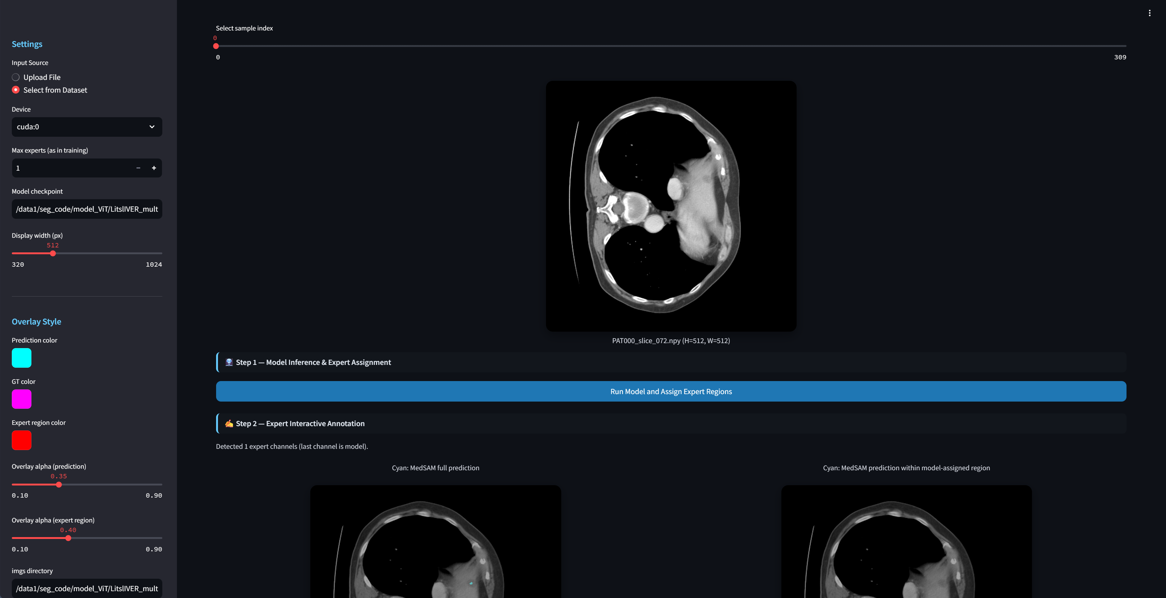
To demonstrate how DeferredSeg supports real expert collaboration, we implement a Streamlit-based interactive interface that replaces the synthetic experts in SynthExpertSeg with human experts at inference time. The interface is organised into three stages (see Fig. 5):

• Step 1 – Model inference & expert assignment. The user uploads a slice (or selects one from the built-in dataset browser). DeferredSeg runs the MedSAM-based segmentor and aggregated deferral predictor to obtain the base prediction and pixel-wise routing scores, and automatically partitions the image into $J$ expert regions plus a model-only region.

• Step 2 – Expert interactive annotation. For each expert region, the interface creates a dedicated canvas that only highlights pixels assigned to that expert. The human expert draws corrections within their own assigned region using freehand tools, providing refined labels exactly where their expertise is requested, while non-assigned areas remain untouched in that canvas.

• Step 3 – Fusion & comparison. The corrected expert masks are fused with the model branch via the same deferral rule as in the main framework, producing a final segmentation mask. The interface visualises the fused result and, when available, overlays the ground-truth mask for qualitative comparison.

A screen-capture video demonstrating the full workflow of this interface (including loading data, assigning expert regions, annotating, and fusing the final result) is provided in the supplementary material.

Figure 5: DeferredSeg interactive expert-annotation interface. The page shows (top) model prediction and routing results, (middle) per-expert canvases for interactive corrections, and (bottom) the fused segmentation and ground-truth comparison.

Appendix B Dataset Details

PROMISE12 The PROMISE12 challenge provides 50 T2-weighted MRI volumes for training and 30 hidden test cases, each annotated with a whole-prostate mask. We resample all volumes to $1\,\text{mm}^{3}$ isotropic voxel spacing. This dataset targets single-organ segmentation in MRI and serves as a testbed for assessing deferral sensitivity near ambiguous prostate boundaries.

LiTS The LiTS challenge offers 201 abdominal CT scans, with 131 publicly labeled volumes containing both liver and tumour masks, and 70 held-out cases for blind testing. We clip CT intensities to $[-200,250]$ Hounsfield units(HU) and apply zero-mean, unit-variance normalisation. This dataset tests the model’s ability to balance large-organ and small-lesion segmentation under significant scale disparity.

AMOS22 AMOS22 contains 500 CT and 100 MRI scans, each annotated for 15 abdominal organs. We follow the official split, resample all volumes to $1\,\text{mm}$ isotropic spacing, and clip CT intensities to $[-250,250]$ HU, and normalise MRI volumes via whole-volume min–max scaling. This multi-organ dataset provides a comprehensive setting for evaluating scalability and expert routing in complex anatomical contexts.

Appendix C Full Results of Coherence–Balance grid search

Table 8 reports the complete numerical results for all branches (System / Expert / Model) and metrics (Jaccard / DSC / Sensitivity) across all $\lambda_{1},\lambda_{2}$ combinations.

Table 8: Effect of varying coherence ($\lambda_{1}$) and balance ($\lambda_{2}$) weights on System / Expert / Model performance (%).

Group	$\lambda_{1}$	$\lambda_{2}$	System			Expert			Model
			Jaccard	DSC	Sens.	Jaccard	DSC	Sens.	Jaccard	DSC	Sens.
A	0.10	0.10	91.26	95.35	94.74	87.45	93.21	91.99	92.71	93.32	98.55
B	0.10	1.00	91.12	95.25	94.73	87.51	93.25	92.00	93.80	94.43	99.90
C	0.10	5.00	91.04	95.11	94.76	87.42	93.09	91.99	93.66	94.47	95.20
D	0.10	10.00	91.36	95.43	94.67	87.89	93.50	92.02	93.12	93.95	99.23
E	1.00	0.10	91.37	95.44	94.66	87.96	93.54	91.99	93.02	93.84	99.39
F	1.00	1.00	90.74	95.02	94.66	87.08	92.97	91.97	93.85	94.59	99.45
G	1.00	5.00	91.90	95.63	96.13	88.48	93.73	93.98	93.20	94.32	94.86
H	1.00	10.00	91.03	95.21	94.70	87.27	93.09	92.01	93.47	94.21	98.91
I	5.00	0.10	90.28	94.61	94.77	86.43	92.41	92.00	93.70	94.44	99.59
J	5.00	1.00	91.63	95.58	94.83	87.90	93.50	92.01	92.57	93.30	99.09
K	5.00	5.00	91.12	95.22	94.66	87.71	93.33	91.99	93.71	94.51	95.02
L	5.00	10.00	91.64	95.59	94.60	88.22	93.69	92.01	91.76	92.42	99.24
M	10.00	0.10	91.30	95.36	94.64	87.88	93.45	92.01	92.14	92.94	98.18
N	10.00	1.00	91.13	95.28	94.62	87.65	93.35	91.98	92.20	93.19	98.39
O	10.00	5.00	91.22	95.34	94.68	87.64	93.32	92.01	94.06	94.88	99.49
P	10.00	10.00	90.53	94.87	94.68	86.91	92.84	92.00	90.66	91.32	99.55

Full Heatmaps: For completeness, Fig. 6 shows the nine heatmaps spanning all branches (System / Expert / Model) and metrics (Jaccard / DSC / Sensitivity).

Figure 6: Complete set of heatmaps for all branches and metrics.

Appendix D Expert Scalability Analysis

For the scalability experiments, each expert set is drawn from a fixed pool of five synthetic experts (E1–E5), respectively (see Tab. 9), while keeping the overall FG/BG accuracy approximately constant across groups. Specifically:

• 1 expert uses E1.

• 2 experts use E2, E3.

• 3 experts use E1, E2, E3.

• 4 experts use E2, E3, E4, E5.

• 5 experts use E1, E2, E3, E4, E5.

And the complete System/Expert/Model scores are provided in Tab. 10

Table 9: Settings of standard synthetic experts used in the scalability experiment (FG, BG, BD).

Expert	FG	BG	BD (edge boost)
E1	0.92	0.98	0.05
E2	0.91	0.99	0.05
E3	0.93	0.97	0.05
E4	0.90	0.97	0.10
E5	0.94	0.99	0.06

Table 10: Performance on PROMISE12 under different numbers of experts (%). Single expert yields peak overlap (DSC/Jaccard), whereas multiple experts raise Sensitivity. (mean $\pm$ std; row-wise best in bold, second best in italics)

Metric	Predictor	J = 1	J = 2	J = 3	J = 4	J = 5
DSC	System	97.06 $\pm$ 0.05	94.48 $\pm$ 0.49	96.00 $\pm$ 0.14	94.43 $\pm$ 0.52	95.45 $\pm$ 0.31
	Expert	97.88 $\pm$ 0.01	92.08 $\pm$ 0.72	95.09 $\pm$ 0.19	93.05 $\pm$ 0.57	93.48 $\pm$ 0.27
	Model	82.80 $\pm$ 2.75	92.14 $\pm$ 2.60	87.17 $\pm$ 1.99	82.44 $\pm$ 0.61	91.45 $\pm$ 1.84
Jaccard	System	94.38 $\pm$ 0.08	89.65 $\pm$ 0.83	92.46 $\pm$ 0.24	89.63 $\pm$ 0.89	91.44 $\pm$ 0.64
	Expert	95.85 $\pm$ 0.01	85.42 $\pm$ 1.20	90.80 $\pm$ 0.32	87.16 $\pm$ 0.96	87.94 $\pm$ 0.94
	Model	79.56 $\pm$ 2.68	91.05 $\pm$ 2.30	86.80 $\pm$ 1.91	82.24 $\pm$ 0.61	90.71 $\pm$ 1.62
Sens.	System	95.33 $\pm$ 0.09	94.08 $\pm$ 0.13	96.42 $\pm$ 0.04	94.76 $\pm$ 0.06	96.64 $\pm$ 0.11
	Expert	97.01 $\pm$ 0.00	91.07 $\pm$ 0.01	95.57 $\pm$ 0.04	93.29 $\pm$ 0.08	95.00 $\pm$ 0.06
	Model	83.55 $\pm$ 1.37	99.21 $\pm$ 0.43	99.05 $\pm$ 0.64	99.75 $\pm$ 0.25	91.95 $\pm$ 0.19

Appendix E Complementary Expert Settings and Detailed Results

To analyze the impact of complementary expert configurations, we define seven synthetic experts with distinct accuracy profiles on FG, BG, and BD regions (Tab. 11). By selecting different subsets of these experts, we emulate varying levels of complementarity and specialization.

Table 11: Accuracy profiles of complementary experts.

Expert Type	FG	BG	BD
(E1) FG strong	0.97	0.90	0.08
(E2) BG strong	0.88	0.99	0.08
(E3) BD strong	0.88	0.90	0.12
(E4) FG+BG strong	0.97	0.99	0.03
(E5) FG+BD strong	0.97	0.90	0.10
(E6) BG+BD strong	0.88	0.99	0.12
(E7) FG+BG+BD strong	0.97	0.99	0.03

Table 12 presents the detailed performance of System / Expert / Model branches as the number of complementary experts increases. A single complementary expert (J=1) already achieves high System performance. Adding three or more complementary experts (J=3–5) further improves System Jaccard and DSC, with the strongest results obtained at J=5 (Tab. 12).

Table 12: System / Expert / Model performance with increasing number of complementary experts (mean $\pm$ std, %).

J	Experts	System			Expert			Model
		Jaccard	DSC	Sens.	Jaccard	DSC	Sens.	Jaccard	DSC	Sens.
1	E1	91.04 $\pm$ 0.16	95.24 $\pm$ 0.10	95.54 $\pm$ 0.06	91.00 $\pm$ 0.19	95.21 $\pm$ 0.10	97.01 $\pm$ 0.02	80.81 $\pm$ 2.70	83.94 $\pm$ 2.84	85.12 $\pm$ 1.20
2	E1, E6	89.03 $\pm$ 0.72	94.10 $\pm$ 0.42	93.58 $\pm$ 0.81	91.91 $\pm$ 0.09	95.73 $\pm$ 0.05	97.04 $\pm$ 0.00	84.07 $\pm$ 5.16	80.63 $\pm$ 5.01	91.85 $\pm$ 2.05
3	E1, E2, E3	92.45 $\pm$ 0.21	95.99 $\pm$ 0.13	96.38 $\pm$ 0.05	90.73 $\pm$ 0.26	95.05 $\pm$ 0.15	95.51 $\pm$ 0.01	85.21 $\pm$ 2.68	85.59 $\pm$ 2.66	98.76 $\pm$ 0.97
4	E1, E2, E3, E4	94.06 $\pm$ 0.46	96.83 $\pm$ 0.18	97.43 $\pm$ 0.04	92.02 $\pm$ 0.18	95.50 $\pm$ 0.12	96.94 $\pm$ 0.01	74.45 $\pm$ 3.00	74.62 $\pm$ 2.98	99.50 $\pm$ 0.44
5	E1, E2, E3, E4, E5	94.40 $\pm$ 0.45	96.88 $\pm$ 0.26	97.46 $\pm$ 0.07	93.13 $\pm$ 0.36	96.39 $\pm$ 0.21	96.92 $\pm$ 1.42	78.31 $\pm$ 78.58	14.99 $\pm$ 23.13	98.48 $\pm$ 0.03

References

- [1] (2008) Classification with a reject option using a hinge loss.. JMLR. Cited by: §2.2.
- [2] (2023) The liver tumor segmentation benchmark (lits). MedIA. Cited by: Table 1.
- [3] (2025) CENet: context enhancement network for medical image segmentation. MICCAI. Cited by: §5.3.1.
- [4] (2022) Swin-unet: unet-like pure transformer for medical image segmentation. In ECCV, Cited by: §1, §2.1.2.
- [5] (2001) Active contours without edges. IEEE TIP. Cited by: §1, §2.1.1.
- [6] (2024) Learning robust shape regularization for generalizable medical image segmentation. IEEE TMI. Cited by: §1.
- [7] (2023) Sam-adapter: adapting segment anything in underperformed scenes. In ICCV, Cited by: §2.1.3.
- [8] (2016) Learning with rejection. In ALT, Cited by: §3.2.
- [9] (2020) Regression under human assistance. In AAAI, Cited by: §2.2.
- [10] (2021) Classification under human assistance. In AAAI, Cited by: §1, §2.2.
- [11] (2025) Confounding-robust deferral policy learning. In AAAI, Cited by: §2.2.
- [12] (2025) Survey on leveraging uncertainty estimation towards trustworthy deep neural networks: the case of reject option and post-training processing. ACM COMPUT SURV. Cited by: §1.
- [13] (2022) Unetr: transformers for 3d medical image segmentation. In WACV, Cited by: §1, §2.1.2.
- [14] (2023) H2former: an efficient hierarchical hybrid transformer for medical image segmentation. IEEE TMI. Cited by: §1.
- [15] (2022) Missformer: an effective transformer for 2d medical image segmentation. IEEE TMI. Cited by: §2.1.2.
- [16] (2021) NnU-net: a self-configuring method for deep learning-based biomedical image segmentation. Nature methods. Cited by: §2.1.2.
- [17] (2024) Nnu-net revisited: a call for rigorous validation in 3d medical image segmentation. In MICCAI, Cited by: §5.3.1.
- [18] (2022) Amos: a large-scale abdominal multi-organ benchmark for versatile medical image segmentation. NeurIPS. Cited by: Table 1.
- [19] (2021) Scaling up visual and vision-language representation learning with noisy text supervision. In ICML, Cited by: §2.1.3.
- [20] (2017) Efficient multi-scale 3d cnn with fully connected crf for accurate brain lesion segmentation. MedIA. Cited by: §1, §2.1.2.
- [21] (2023) Segment anything. In ICCV, Cited by: §2.1.3.
- [22] (2024) Efficiently correcting patch-based segmentation errors to control image-level performance in retinal images. In MIDL, Cited by: §2.1.2.
- [23] (2024) Confidence calibration of classifiers with many classes. NeurIPS. Cited by: §1.
- [24] (2025) Uncertainty weighted gradients for model calibration. In CVPR, Cited by: §1.
- [25] (2017) A survey on deep learning in medical image analysis. MedIA. Cited by: §1, §2.1.2.
- [26] (2014) Evaluation of prostate segmentation algorithms for mri: the promise12 challenge. MedIA. Cited by: Table 1.
- [27] (2024) Mitigating underfitting in learning to defer with consistent losses. In AISTATS, Cited by: §2.2.
- [28] (2022) Transforming the interactive segmentation for medical imaging. In MICCAI, Cited by: §1, §2.1.2.
- [29] (2015) Fully convolutional networks for semantic segmentation. In CVPR, Cited by: §2.1.2.
- [30] (2022) Bridging the gap between vision transformers and convolutional neural networks on small datasets. NeurIPS. Cited by: §1, §4.2.3.
- [31] (2021) MIDeepSeg: minimally interactive segmentation of unseen objects from medical images using deep learning. MIA 72, pp. 102102. Cited by: §1, §2.1.2.
- [32] (2024) Segment anything in medical images. Nature Communications. Cited by: §2.1.3.
- [33] (2018) Predict responsibly: improving fairness and accuracy by learning to defer. NeurIPS. Cited by: §1, §2.2.
- [34] (2023) Two-stage learning to defer with multiple experts. NeurIPS. Cited by: §2.2.
- [35] (2024) Regression with multi-expert deferral. ICML. Cited by: §2.2.
- [36] (2020) Confidence calibration and predictive uncertainty estimation for deep medical image segmentation. IEEE TMI. Cited by: §1.
- [37] (2016) V-net: fully convolutional neural networks for volumetric medical image segmentation. In 3DV, Cited by: §1, §2.1.2.
- [38] (2020) Consistent estimators for learning to defer to an expert. In ICML, Cited by: §1, §2.2.
- [39] (2024) Benchmarking uncertainty disentanglement: specialized uncertainties for specialized tasks. NeurIPS. Cited by: §1.
- [40] (2025) Probabilistic learning to defer: handling missing expert annotations and controlling workload distribution. In ICLR, Cited by: §2.2.
- [41] (2021) Differentiable learning under triage. NeurIPS. Cited by: §1, §2.2.
- [42] (2018) Attention u-net: learning where to look for the pancreas. MIDL. Cited by: §1, §2.1.2.
- [43] (2021) Learning transferable visual models from natural language supervision. In ICML, Cited by: §2.1.3.
- [44] (2015) U-net: convolutional networks for biomedical image segmentation. In MICCAI, Cited by: §1, §2.1.2.
- [45] (2004) Survey over image thresholding techniques and quantitative performance evaluation. J. Electron. Imaging. Cited by: §2.1.1.
- [46] (2000) Normalized cuts and image segmentation. IEEE TPAMI. Cited by: §1, §2.1.1.
- [47] (2021) Reinforcement learning under algorithmic triage. arXiv preprint arXiv:2109.11328. Cited by: §2.2.
- [48] (2024) Towards human-ai collaboration in healthcare: guided deferral systems with large language models. In ICML, Cited by: §1, §2.2.
- [49] (2023) Learning to defer to multiple experts: consistent surrogate losses, confidence calibration, and conformal ensembles. In AISTATS, pp. 11415–11434. Cited by: §1, §2.2.
- [50] (2022) Calibrated learning to defer with one-vs-all classifiers. In ICML, Cited by: §2.2.
- [51] (2022) Medical image segmentation using deep learning: a survey. IET image processing. Cited by: §1.
- [52] (2024) Exploiting human-ai dependence for learning to defer. In ICML, Cited by: §1.
- [53] (2022) SAM: self-supervised learning of pixel-wise anatomical embeddings in radiological images. IEEE TMI. Cited by: §2.1.3.
- [54] (2025) Segment together: a versatile paradigm for semi-supervised medical image segmentation. IEEE TMI. Cited by: §2.1.1.
- [55] (2018) Unet++: a nested u-net architecture for medical image segmentation. In DLMIA/ML-CDS 2018 @ MICCAI, Cited by: §2.1.2.