TRACE: Capability-Targeted Agentic Training

Abstract

Models fail to complete agentic tasks often due to missing core capabilities. However, mainstream approaches for addressing these failures often rely on fine-tuning directly on the target environments or generating synthetic data that is not targeted to the model’s actual capability deficits, resulting in low sample efficiency and limited generalizability. We introduce TRACE (Turning Recurrent Agent failures into Capability-targeted training Environments), an end-to-end system for environment-specific agent self-improvement. TRACE contrasts successful and failed trajectories to automatically identify lacking capabilities, synthesizes a targeted training environment for each that rewards whether the capability was exercised, trains a LoRA adapter via RL on each synthetic environment, and then trains a mixture-of-experts (MoE) model over the capability adapters. TRACE can be effectively applied across different environments, improving over the base agent by +15.3 points on $\tau^{2}$-Bench (customer service) and +15 points Pass@1 on SWE-bench Verified (software engineering), outperforming the strongest external baselines, GEPA and SWE-RL, by +8.6 points and +8.4 points, respectively. In addition, TRACE is more sample-efficient than strong finetuning baselines: using less than one-fourth the number of rollouts, TRACE outperforms the best-performing baselines, GRPO and GEPA, and achieves higher final accuracy by +10.4 and +8.6 points on $\tau^{2}$-Bench. The code is available at https://github.com/ScalingIntelligence/TRACE.git.

1 Introduction

(a) Qwen3-30B-A3B-Instruct

(b) Qwen3.6-27B

Figure 1: TRACE outperforms the base agent and all baselines on both $\tau^{2}$-Bench (overall pass rate) and SWE-bench Verified Verified (Pass@1), across two agent backbones.

Large Language Models (LLMs) are increasingly deployed in agentic environments, such as customer-service workflows (Yao et al., 2024) and coding platforms (Jimenez et al., 2024; Xu et al., 2025), where they must complete multi-step tasks through tool use, reasoning, and interaction with an environment. When models fail in these settings, their failures are often not isolated to a single task instance. Instead, they frequently reflect missing core capabilities that are required across many different tasks. We define a capability as performing one or more actions in a trajectory that are necessary for successfully solving some subset of task instances in the target environment. For example, in a customer-service environment, retrieving the correct customer record is a capability necessary for tasks such as canceling a flight, changing a seat, or verifying a reservation.

A natural approach to improving an LLM in a target agentic environment is to finetune it directly on that environment using Reinforcement Learning (RL) or Supervised Fine-Tuning (SFT). However, direct training on the target environment often provides supervision only at the level of task outcomes or task-specific trajectories. This training signal does not explicitly reveal which underlying capabilities the agent lacks. As a result, the model must implicitly infer shared capabilities from sparse and heterogeneous task-level feedback, making learning sample-inefficient and limiting generalization across task instances.

Another line of work scales synthetic RL environments and training data (Sullivan et al., 2025; Wang et al., 2026a; Fang et al., 2025a; Tu et al., 2026; Song et al., 2026a). While these approaches increase the amount and diversity of training data, the generated data is often not targeted to the model’s actual capability deficits in the target environment. Consequently, training may spend substantial compute on behaviors the model already performs well or on capabilities that are irrelevant to the target failures, yielding limited sample efficiency and weak environment-specific improvement.

Figure 2: Overview of TRACE, an end-to-end system for automated environment-specific agent self-improvement. TRACE automatically identifies the specific capabilities that an agent lacks and synthesizes targeted training environments for each capability.

In this work, we introduce TRACE (Turning Recurrent Agent failures into Capability-targeted training Environments), an end-to-end system for environment-specific agent self-improvement. Rather than training directly on the target environment or relying on untargeted synthetic data, TRACE uses the agent’s own successful and failed trajectories to identify the capabilities whose absence explains recurring failures. It then synthesizes capability-targeted training environments that isolate and reward exercising each missing capability, trains a LoRA adapter via RL on each synthetic environment, and composes the resulting adapters through a Mixture-of-Experts (MoE) model.

TRACE is designed around three objectives:

1. Identifying high-impact capability deficits. The agent may fail for many reasons, so it is important to automatically determine which missing capabilities most clearly distinguish failed trajectories from successful ones and prioritize those that account for the largest number of failures.

2. Synthesizing capability-targeted training environments. For each identified deficit, the agent needs a training environment that directly isolates and rewards exercising the missing capability while preserving the target environment’s interface.

3. Learning and composing multiple capabilities. The agent must acquire multiple identified capabilities from their respective synthetic environments and apply the appropriate capabilities to each task instance in the target environment.

Figure 2 shows an overview of TRACE, which consists of four steps. In step 1, the base agent generates rollouts in the target environment, and an LLM-based analysis agent contrasts successful and failed trajectories to identify capabilities that meaningfully distinguish the two, ranking them by failure coverage. In step 2, for each retained capability, an LLM-based generation agent uses the capability description and corresponding failed trajectories to construct a synthetic environment that isolates the missing capability while preserving the target environment’s interface, such as its tool schemas, interaction protocol, and output format. Task instances are procedurally generated from random seeds, and whether the capability is exercised is verified automatically from tool arguments, state changes, or final outputs. In step 3, we train a LoRA adapter on each capability-specific synthetic environment using RL. In step 4, we train a Mixture-of-Experts (MoE) (Shazeer et al., 2017) model over the capability adapters.

Our contributions are as follows:

• We propose TRACE, an end-to-end system for environment-specific agent self-improvement. TRACE contrasts successful and failed trajectories from the target environment to automatically identify the specific capabilities the agent lacks, then synthesizes targeted training environments that teach the agent to exercise those capabilities.

• We show that TRACE can be effectively applied across different agentic environments. On $\tau^{2}$-Bench (Barres et al., 2025), a customer-service benchmark, TRACE achieves a 48.2% overall pass rate, improving over the base agent by +15.3 points and outperforming the strongest external baseline, GEPA, by +8.6 points (Table 1). On SWE-bench Verified (Jimenez et al., 2024), a software-engineering benchmark, TRACE reaches 41% Pass@1, improving over the base agent by +15 points and outperforming the strongest external baseline, SWE-RL, by +8.4 points (Table 2). Moreover, with Qwen3.6-27B, TRACE attains 73.2% Pass@1 on SWE-bench Verified Verified, outperforming much larger frontier models, including GPT-5.2-Codex (72.8%), GLM 5, and Claude 4.5 Sonnet, on the public SWE-bench leaderboard, despite using a substantially smaller open-weight model.

• We demonstrate that TRACE is more sample-efficient than strong finetuning baselines. With Qwen3-30B-A3B-Instruct, TRACE uses only 2–4 capability-specific LoRA adapters, each updating only 5.3% of the model parameters, yet improves performance on $\tau^{2}$-Bench by +15.3 points and Pass@1 on SWE-bench Verified by +15 points. In addition, using less than one-fourth the number of rollouts, TRACE outperforms the best-performing baselines, GRPO (Shao et al., 2024) and GEPA (Agrawal et al., 2026), and achieves higher final accuracy by +10.4 and +8.6 points on $\tau^{2}$-Bench, respectively.

• We show that training on capability-targeted environments outperforms only adding capabilities to the prompt. With Qwen3-30B-A3B-Instruct, training on capability-targeted environments yields a +8.6 point improvement on $\tau^{2}$-Bench and +10 point improvement in Pass@1 on SWE-bench Verified over prompt-based optimization (Figure 4(a)).

2 Related Work

LLM Agents and Interactive Environments. Autonomous LLM agents are increasingly deployed in complex, multi-turn environments. Rigorous evaluation requires mastering specific tool interfaces and interaction protocols, driving the adoption of benchmarks like $\tau^{2}$-Bench, SWE-bench (Jimenez et al., 2024), WebArena (Zhou et al., 2024), WorkArena (Drouin et al., 2024), WorkArena++ (Boisvert et al., 2024), Terminal-Bench (Merrill et al., 2026) and TheAgentCompany (Xu et al., 2024).

Agentic Reinforcement Learning and Synthetic Data. Recent alignment methods utilize in-the-wild device control (Bai et al., 2024), implicit step rewards (Liu et al., 2025), or verifiable multi-turn RL (Gao et al., 2026; Zhang et al., 2025). A common capability-acquisition strategy scales training through procedurally synthesized environments (Sullivan et al., 2025) (e.g., AWM (Wang et al., 2026b), EnvScaler (Song et al., 2026a), ScaleEnv (Tu et al., 2026)) or unified public trajectories(e.g. ADP (Song et al., 2026b)). While effective for general capabilities (Yang et al., 2025; Fang et al., 2025b), these approaches overlook model-specific failures. TRACE diverges by using contrastive analysis to identify missing capabilities, synthesizing training environments to isolate and reward correct execution of each capability.

LoRA Merging and Routing. Recent work on model merging has established general techniques for composing task-specific adaptations (Ilharco et al., 2023a; Yadav et al., 2023b; Panariello et al., 2025a). A complementary direction avoids collapsing everything into one checkpoint and instead uses mixtures of LoRA experts, where routing dynamically selects or softly combines experts such as  (Luo et al., 2024; Cao et al., 2026), including foundational LoRA-MoE methods such as LoRAMoE (Dou et al., 2024), MoLE (Wu et al., 2024), and MoV/MoLORA (Zadouri et al., 2024), as well as variants exploring different routing granularities and mergeability (Gao et al., 2024; Zhao et al., 2025). Unlike methods where experts emerge implicitly from multi-task data, TRACE’s adapters are independently trained on synthetic environments that each isolate a single, contrastively identified capability, yielding an interpretable set of experts. Advances in adapter architectures and MoE training schemes are orthogonal to TRACE and can be incorporated into our pipeline for further gains.

3 Method

3.1 Preliminaries

Agentic environment.

We represent an agentic environment as a tuple $\mathcal{E}=(\mathcal{X}_{\mathcal{E}},P_{\mathcal{E}},R_{\mathcal{E}},y_{\mathcal{E}})$, where $\mathcal{X}_{\mathcal{E}}$ is the set of task instances, $P_{\mathcal{E}}$ defines the interaction dynamics, $R_{\mathcal{E}}(x,\tau)$ is a trajectory-level reward and can either be discrete or continuous, and $y_{\mathcal{E}}(x,\tau)\in\{0,1\}$ is a binary label indicating whether $\tau$ succeeded or not.

A task instance $x\sim\mathcal{X}_{\mathcal{E}}$ determines the initial observation $o_{1}$ presented to the agent. An LLM policy $\pi_{\theta}$ then selects actions conditioned on the interaction history $h_{t}=(o_{1},a_{1},\dots,o_{t})$ via $a_{t}\sim\pi_{\theta}(\cdot\mid h_{t})$, where each action is a variable-length token sequence that may include natural-language reasoning and tool calls. The environment returns an observation $o_{t+1}$ after each action, and the episode continues for at most $T$ steps, producing a trajectory $\tau=(o_{1},a_{1},\dots,o_{T},a_{T},o_{T+1})$. At episode end, the environment assigns reward $R_{\mathcal{E}}(x,\tau)$ and success label $y_{\mathcal{E}}(x,\tau)$. We denote by $\mathcal{D}=\{(x_{i},\tau_{i},r_{i},y_{i})\}_{i=1}^{N}$ a dataset of $N$ collected episodes.

Synthetic environment.

A synthetic verifiable environment is an agentic environment $\mathcal{E}_{s}=(G_{\mathcal{E}_{s}},P_{\mathcal{E}_{s}},R_{\mathcal{E}_{s}},y_{\mathcal{E}_{s}})$ whose task instances are produced by an explicit generator $G_{\mathcal{E}_{s}}$ and whose reward and success label can be evaluated automatically from the task instance and trajectory. Concretely, given a random seed $z$, the generator produces a task instance $x_{s}=G_{\mathcal{E}_{s}}(z)$ together with the associated environment configuration, such as the initial state, transition logic, and evaluation criteria. Interaction with $\mathcal{E}_{s}$ then produces a trajectory $\tau_{s}$ with reward $R_{\mathcal{E}_{s}}(x_{s},\tau_{s})$ and success label $y_{\mathcal{E}_{s}}(x_{s},\tau_{s})$. Because both generation and verification are algorithmic, synthetic verifiable environments can be scaled to produce large numbers of training instances with verifiable reward signal.

3.2 Problem Formulation

Our goal is to learn an LLM policy $\pi_{\theta}$ for a target agentic environment $\mathcal{E}$ that maximizes expected return:

$$J(\pi_{\theta};\mathcal{E})\;=\;\mathbb{E}_{x\sim\mathcal{X}_{\mathcal{E}},\,\tau\sim p_{\pi_{\theta}}(\cdot\mid x,\mathcal{E})}\bigl[R_{\mathcal{E}}(x,\tau)\bigr],$$

Here, $x$ is a task instance, $\tau$ is a corresponding trajectory induced by executing $\pi_{\theta}$ in $\mathcal{E}$ on $x$, and $R_{\mathcal{E}}(x,\tau)$ is the trajectory-level reward.

A central challenge is that optimization in the target environment provides limited failure attribution. The policy must infer what is necessary for success across task instances only indirectly from the training signal, making optimization inefficient. We formalize such underlying necessities as capabilities.

Definition 1 (Capability).

A capability consists of performing one or more actions in a trajectory that are necessary for successfully solving some subset of task instances in the environment. For $X_{c}\subseteq X_{\mathcal{E}}$, let $\nu_{c}(x,\tau)=1$ indicate that capability $c$ is exercised in trajectory $\tau$ for task instance $x$. Then, for every $x\in X_{c}$ and a corresponding trajectory $\tau$, $y_{\mathcal{E}}(x,\tau)=1\;\Rightarrow\;\nu_{c}(x,\tau)=1.$

Examples.

1. In a customer-service environment, retrieving the correct customer record is a capability, since it is necessary for tasks such as canceling a flight, changing a seat, or verifying a reservation.

2. In a coding environment, correctly locating the relevant function or file is a capability, since it is necessary for tasks such as fixing a bug, adding a feature, or updating an API call.

However, in $\mathcal{E}$, $R_{\mathcal{E}}(x,\tau)$ does not generally provide an explicit signal of whether $\nu_{c}(x,\tau)=1$ for each capability $c$, making it difficult to isolate and train any single capability directly. To address this, we introduce:

Definition 2 (Capability-targeted synthetic environment).

For a capability $c$, a capability-targeted synthetic environment is a synthetic verifiable environment $\mathcal{E}_{s}^{c}=(G_{c},P_{c},R_{c},y_{c})$ constructed to satisfy three properties:

1. Every task instance $x_{c}$ generated by $G_{c}$ ensures that exercising $c$ is necessary for success.

2. $P_{c}$ preserves the aspects of $P_{\mathcal{E}}$ that are relevant to exercising $c$, such as tool schemas, state representation, and policy constraints.

3. For any $x_{c}$ and a corresponding trajectory $\tau_{c}$, the reward $R_{c}(x_{c},\tau_{c})$ and success label $y_{c}(x_{c},\tau_{c})$ are automatically computable from $(x_{c},\tau_{c})$. Higher reward and success depend primarily on whether $c$ is exercised in $\tau_{c}$.

Because each $\mathcal{E}_{s}^{c}$ isolates a single capability, its reward signal is generally denser and more attributable than that of $\mathcal{E}$. This decomposition reduces the problem of optimizing $J(\pi_{\theta};\mathcal{E})$ to three tractable subproblems: (1) identifying the capabilities that $\pi_{\theta}$ lacks in $\mathcal{E}$, i.e., those for which $\nu_{c}(x,\tau)=0$ across many task instances; (2) synthesizing a capability-targeted environment $\mathcal{E}_{s}^{c}$ for each identified capability; and (3) training $\pi_{\theta}$ on each $\mathcal{E}_{s}^{c}$ to improve performance back in $\mathcal{E}$. In the following subsections, we describe TRACE, an end-to-end self-improving system that tackles each of these subproblems.

3.3 Automated Capability-Targeted Synthetic Environment Generation Pipeline

Given a representative dataset $\mathcal{D}=\{(x_{i},\tau_{i},r_{i},y_{i})\}_{i=1}^{N}$ collected by rolling out $\pi_{\theta}$ in the target environment $\mathcal{E}$, TRACE introduces an agentic pipeline that automatically: (i) identifies capabilities that distinguish failed trajectories from successful ones and (ii) constructs a capability-targeted synthetic environment for each.

Contrastive capability identification. Given $\mathcal{D}$, our goal is to identify capabilities that $\pi_{\theta}$ lacks and prioritize those responsible for a substantial fraction of failures, so that they can be targeted for training. We first split $\mathcal{D}$ into successful and failed subsets according to the success label $y_{i}$: $\mathcal{D}^{+}=\{(x_{i},\tau_{i},r_{i},y_{i})\in\mathcal{D}\mid y_{i}=1\}$ and $\mathcal{D}^{-}=\{(x_{i},\tau_{i},r_{i},y_{i})\in\mathcal{D}\mid y_{i}=0\}$.

Then, to ensure capability definitions remain consistent across multiple independent analysis runs, we structure the identification process into two phases: discovery and labeling. First, in the discovery phase, an LLM-based analysis agent examines the tool calls, tool results, and final responses across the trajectories to induce a canonical dictionary of candidate recurring capabilities $\mathcal{C}$. Each capability $c\in\mathcal{C}$ is assigned a fixed name and natural-language description. Second, in the labeling phase, the analysis agent uses this fixed dictionary to systematically evaluate the dataset. For each trajectory $\tau_{i}$ and capability $c\in\mathcal{C}$, the agent predicts a label $\ell_{c}(x_{i},\tau_{i})\in\{\texttt{NA},\texttt{PRESENT},\texttt{LACKING}\}$. Here, NA means the analysis agent predicts $x_{i}\notin X_{c}$ ($c$ is not necessary for $x_{i}$), PRESENT means the analysis agent predicts $x_{i}\in X_{c}$ and $\nu_{c}(x_{i},\tau_{i})=1$ ($c$ is necessary for $x_{i}$ and exercised in $\tau_{i}$), and LACKING means the analysis agent predicts $x_{i}\in X_{c}$ and $\nu_{c}(x_{i},\tau_{i})=0$ ($c$ is necessary for $x_{i}$ but not exercised in $\tau_{i}$). For each capability $c\in\mathcal{C}$, we estimate its error rate on successful and failed trajectories:

Let $\ell_{i}^{c}:=\ell_{c}(x_{i},\tau_{i})$. Then

$$\widehat{\mathrm{ER}}^{+}(c) =\frac{\sum_{i}\mathbf{1}\!\left[\ell_{i}^{c}=\textsc{Lacking},\,y_{i}=1\right]}{\sum_{i}\mathbf{1}\!\left[\ell_{i}^{c}\neq\textsc{NA},\,y_{i}=1\right]},$$

$$\widehat{\mathrm{ER}}^{-}(c) =\frac{\sum_{i}\mathbf{1}\!\left[\ell_{i}^{c}=\textsc{Lacking},\,y_{i}=0\right]}{\sum_{i}\mathbf{1}\!\left[\ell_{i}^{c}\neq\textsc{NA},\,y_{i}=0\right]}.$$

We then define the contrastive gap as $\widehat{\Delta}(c)=\widehat{\mathrm{ER}}^{-}(c)-\widehat{\mathrm{ER}}^{+}(c).$ which measures how much more often $c$ is lacking in failed trajectories than in successful ones. This contrastive criterion is more robust than analyzing failures alone: it filters out capabilities with uniformly low success rates, which often reflect task ambiguity or annotation noise rather than a trainable deficit, and it excludes capabilities that occasionally fail but do not meaningfully distinguish successful from unsuccessful trajectories.

We also compute the coverage of each capability over failed trajectories $\widehat{\mathrm{Cov}}(c)=1/|\mathcal{D}^{-}|\sum_{i=1}^{N}\mathbf{1}[\ell_{c}(x_{i},\tau_{i})=\textsc{Lacking}\wedge y_{i}=0]$ and retain $\mathcal{C}^{*}=\{c\in\mathcal{C}\mid\widehat{\Delta}(c)\geq\delta,\widehat{\mathrm{Cov}}(c)\geq\rho\}$, representing capabilities that are both strongly contrastive and cover a substantial fraction of failures.

To improve robustness, we repeat the analysis except the discovery step multiple times and retain only capabilities selected consistently across runs. In our experiments, one analysis pass takes approximately $5$ minutes, which is marginal compared to training overhead. We set $\rho=0.10$ (a retained capability must account for at least $10\%$ of failed trajectories) and $\delta=0.20$ (its error rate must be at least $20$ percentage points higher on failed than on successful trajectories). We analyze and provide examples of the identified capabilities in Section 4.3 and Appendix J.

Environment synthesis. For each retained capability $c\in\mathcal{C}^{*}$, an LLM-based generation agent synthesizes a complete training environment $\mathcal{E}_{s}^{c}$. The agent receives the description of $c$ together with the failure patterns identified during contrastive analysis, and produces a seeded task generator $G_{c}$, transition logic, and evaluation criteria that together define $\mathcal{E}_{s}^{c}$ while preserving the target environment’s tool schemas, state representation, and policy constraints. Given a random seed $z$, the generator deterministically constructs a task instance $x=G_{c}(z)$, including synthetic user profiles, database records, and task-specific parameters, so that each seed yields a distinct scenario, preventing memorization and enabling diversity.

By construction, task success in $\mathcal{E}_{s}^{c}$ depends primarily on exercising $c$, which is verified automatically from tool arguments, state changes, or final outputs. For example, if $c$ is structured data reasoning, the environment generates scenarios requiring the agent to search, filter, and cross-reference specific records within complex JSON databases (such as locating a specific flight routing or matching a retail item variant). For each seeded instance, the environment also generates a corresponding ground-truth solution. For that instance, the agent interacts in a multi-turn setting, using tools to query records, modify the database, and converse with a simulated user. The reward is computed by comparing the final database state against the ground truth using hash-based consistency checks and by verifying that the agent communicates the correct final result. Because each environment isolates a single capability, the reward $R_{\mathcal{E}_{s}^{c}}$ is denser and more attributable than that of the original environment, where success may depend on many capabilities at once. Examples of synthesized environments and the generation prompt are in Appendix E and Appendix K.

3.4 Acquiring Capabilities via Reinforcement Learning

Given the family of synthetic environments $\{\mathcal{E}_{s}^{c}\}_{c\in\mathcal{C}^{*}}$ produced by the generation pipeline (§3.3), we train a separate low-rank adapter $\Delta_{c}$  (Hu et al., 2021) for each capability $c\in\mathcal{C}^{*}$ while keeping the base policy $\pi_{\theta}$ frozen.

We optimize each adapter with GRPO, a value-free on-policy algorithm. At each iteration, $\pi_{\theta+\Delta_{c}}$ generates $G$ groups of rollouts in $\mathcal{E}_{s}^{c}$. Within each group $g$, $K$ trajectories $\{\tau_{g,1},\dots,\tau_{g,K}\}$ are sampled from the same seed $z_{g}$, so all rollouts share an identical initial state and differ only through stochastic decoding. Let $r_{g,k}=R_{c}(x_{g},\tau_{g,k})$ denote the reward function, where $x_{g}=G_{c}(z_{g})$. GRPO normalizes rewards within each group to obtain a trajectory-level advantage: $\hat{A}_{g,k}=\frac{r_{g,k}-\bar{r}_{g}}{\sigma_{g}+\epsilon}$, where $\bar{r}_{g}$ and $\sigma_{g}$ are the within-group mean and standard deviation and $\epsilon$ is a small constant for numerical stability. This normalization makes the training signal invariant to reward scale across environments. Because reward is assigned at the trajectory level, all tokens in a rollout share the same advantage; groups in which all rollouts receive identical rewards are discarded, as they carry no learning signal. The adapter is then updated via the standard clipped surrogate objective (Schulman et al., 2017); full details are provided in Appendix A.

3.5 Composing Acquired Capabilities

The target environment $\mathcal{E}$ may require different capabilities across task instances. We consequently train a Mixture-of-Experts (MoE) model over the capability adapters.

We construct the MoE by composing the capability-specific adapters $\{\Delta_{c}\}_{c\in\mathcal{C}^{*}}$ at each adapted transformer block using token-level routing  Dou et al. (2024); Wu et al. (2024); Shazeer et al. (2017). At each adapted block $\ell$, we stack the LoRA factors $\{(A_{c},B_{c})\}_{c\in\mathcal{C}^{*}}$ into a shared adapter bank and introduce a lightweight linear gate $g_{\ell}$. For capability $c$, let $\Delta W_{c}=B_{c}A_{c}$ denote its low-rank weight update. Given hidden state $h$ at block $\ell$, the gate produces capability weights $p_{\ell,c}(h)=\mathrm{softmax}(g_{\ell}(h))_{c}$. For an adapted projection with frozen base weight $W$, the token-dependent update is

$$\Delta W_{\ell}(h)=\sum_{c\in\mathcal{C}^{*}}p_{\ell,c}(h)\,\Delta W_{c},$$

and the projection output is $(W+\Delta W_{\ell}(h))h$. The base policy $\pi_{\theta}$ and all adapters are frozen; only the gates $\{g_{\ell}\}$ are trained. We train the gates with the objective

$$\mathcal{L}=\mathcal{L}_{\mathrm{CE}}+\lambda_{\mathrm{LB}}\,\mathcal{L}_{\mathrm{LB}},$$

where $\mathcal{L}_{\mathrm{CE}}$ is the token-level cross-entropy on the agent’s response tokens and $\mathcal{L}_{\mathrm{LB}}=|\mathcal{C}^{*}|\sum_{c\in\mathcal{C}^{*}}f_{c}\,P_{c}$ is a load-balancing penalty that discourages expert collapse. Here, $f_{c}$ is the fraction of batch tokens for which $c$ has the largest gate probability, $P_{c}$ is the average gate probability assigned to $c$, and $\lambda_{\mathrm{LB}}$ controls the strength of the regularizer. At inference, each token uses the single capability with the largest gate probability. We empirically compare this MoE composition against alternative consolidation strategies (adapter merging, multi-capability GRPO, SFT, and on-policy distillation) in Appendix C.

4 Experiments

4.1 Experimental Setup

Benchmarks & Evaluation. We evaluate on $\tau^{2}$-Bench (Barres et al., 2025) (using the 50 Airline and 114 Retail domains) to test policy-sensitive customer-service workflows, and SWE-bench Verified (Jimenez et al., 2024) (500 instances) to test software-engineering tasks that require resolving real GitHub issues. On $\tau^{2}$-Bench, we report pass rate, the fraction of tasks satisfying the benchmark’s binary success criterion (correct task execution and correct user communication), broken out by the Airline and Retail domains and aggregated over the union of both. On SWE-bench Verified, we report Pass@1, the fraction of instances whose generated patch resolves the issue and passes the held-out tests; all methods, including TRACE’s capability discovery and synthetic environment generation, train on the disjoint SWE-smith (Yang et al., 2025) split. Formal metric definitions are in Appendix F. We additionally evaluate on ToolSandBox (Lu et al., 2025), a stateful tool-use benchmark, in Appendix B. Unless specified otherwise, we evaluate all models with greedy decoding (temperature $0.0$) for deterministic head-to-head comparison, a maximum context length of 32,000 tokens, and a maximum of 50 interaction steps per episode.

Training Hyperparameters. We evaluate with two agent backbones, Qwen3-30B-A3B-Instruct-2507 (Team, 2025) and Qwen3.6-27B (Qwen Team, 2026) (Table 1), optimizing with LoRA and GRPO. On $\tau^{2}$-Bench, the 4 capabilities trained are structured data reasoning, multi-step task completion, precondition verification, and tool calling precision. On SWE-bench Verified, we train 3 capability-targeted synthetic environments. We optimize with AdamW ($\text{lr}=10^{-5}$) for up to 40 iterations per capability, using a sampling temperature of $1.0$ for rollouts. Training utilizes gradient checkpointing and distributed data parallelism across 4–8 A100-80GB GPUs. MoE training uses a load balancing loss coefficient $\lambda_{\mathrm{LB}}=0.05$. As detailed in Appendix D, each LoRA adapter introduces $\sim\!1.6$ B trainable parameters ($5.3\%$ of the backbone), and the trained MoE gate adds $491{,}760$ parameters in total.

Baselines. We compare against direct GRPO training on the target environment, Agent World Model (AWM), which performs RL in benchmark-independent synthetic environments for broad tool-use training, and Agent Data Protocol (ADP), which performs supervised fine-tuning on diverse public agent trajectories in a unified representation. On SWE-bench Verified, we additionally compare against SWE-RL (Wei et al., 2025), a reinforcement learning method specialized for software-engineering agents.

To test whether dedicated training on the identified capabilities is necessary, we compare against the inference-time evolutionary prompt optimization method GEPA. We provide the capabilities identified by TRACE to GEPA and allow it to refine their natural-language descriptions, which are then added to the agent’s system prompt. GEPA optimizes these descriptions for the agent’s pass rate in the target environment. All training baselines and GEPA are run under matched training budgets to ensure fair comparison with TRACE.

Table 1: Pass rate on $\tau^{2}$-Bench with two agent backbones. TRACE outperforms all baselines under both Qwen3-30B-A3B and Qwen3.6-27B.

Model	Method	Airline (%)	Retail (%)	Overall (%)
Qwen3-30B-A3B	Base	24.0	36.8	32.9
	GRPO on Target	32.0	40.4	37.8
	ADP	28.0	34.2	32.3
	AWM	32.0	41.2	38.4
	GEPA	38.0	40.4	39.6
	Single Capability GRPO (Ours)	34.0	43.0	40.3
	TRACE (Ours)	44.0	50.0	48.2
Qwen3.6-27B	Base	60.0	45.6	50.0
	GRPO on Target	66.0	48.2	53.7
	ADP	56.0	49.1	51.2
	GEPA	66.0	47.4	53.0
	Single Capability GRPO (Ours)	66.0	50.8	55.4
	TRACE (Ours)	74.0	52.6	59.1

Table 2: Pass@1 on SWE-bench Verified (500 instances) with two agent backbones.

Model	Method	Pass@1 (%)
Qwen3-30B-A3B	Base	26.0
	ADP	30.2
	GEPA	31.0
	SWE-RL	32.6
	Single Capability GRPO (Ours)	36.6
	TRACE (Ours)	41.0
Qwen3.6-27B	Base	68.0
	ADP	68.4
	GEPA	69.6
	SWE-RL	70.4
	Single Capability GRPO (Ours)	71.0
	TRACE (Ours)	73.2

(a) Capability selection frequency across 10 independent runs. The analysis agent consistently recovers the same top four deficits (green) for targeted training.

(b) Median task failure coverage across runs (error bars denote IQR). Coverage is not mutually exclusive, as a single failed task may lack multiple capabilities.

Figure 3: Stability and coverage of identified capabilities. Repeated contrastive analysis consistently identifies a small, stable set of capability deficits (a) that account for a heavily concentrated proportion of benchmark failures (b). This skewed distribution demonstrates that a few high-impact capabilities drive most errors, validating our use of targeted synthetic environments.

4.2 Effectiveness of Method

Tables 1 and 2 summarize the main experimental results. TRACE consistently outperforms baselines across both evaluated benchmarks, notably improving upon the base model by +15.3 points on $\tau^{2}$-Bench and +15 points Pass@1 on SWE-bench Verified, while beating the strongest external baselines by +8.6 points and +8.4 points, respectively. The same pattern holds with a stronger Qwen3.6-27B backbone on $\tau^{2}$-Bench (Table 1): TRACE reaches a 59.1% overall pass rate, +9.1 points over the base model and +5.4 points over the strongest baseline. On SWE-bench Verified Verified, the Qwen3.6-27B variant of TRACE reaches 73.2% Pass@1 (Table 2), outperforming much larger frontier models, including GPT-5.2-Codex, GLM 5, and Claude 4.5 Sonnet on the public SWE-bench leaderboard.

Targeted vs. General-Purpose Training Environments. A single adapter trained on one synthesized capability environment achieves 40.3% on $\tau^{2}$-Bench and 36.6% Pass@1 on SWE-bench Verified. This surpasses large-scale general-purpose methods such as AWM (38.4% on $\tau^{2}$-Bench) and ADP (32.3% on $\tau^{2}$-Bench, 30.2% on SWE-bench Verified). Notably, ADP’s performance in the $\tau^{2}$-Bench Retail domain is lower than the base model (34.2% vs. 36.8%). These results suggest that diagnosing specific missing capabilities and training on targeted synthetic environments yields higher performance than general-purpose training data.

Capability Training vs. Prompt Optimization. We evaluate the need for dedicated training versus injecting capability descriptions into the prompt optimized with GEPA. As shown in Tables 1 and 2, GEPA improves over the base model on both $\tau^{2}$-Bench (overall pass rate) and SWE-bench Verified (Pass@1). However, it underperforms compared to training a single capability and TRACE with all capabilities on both benchmarks. This demonstrates that while prompting capability instructions is helpful, explicitly training the model to exercise those capabilities is necessary for stronger performance.

4.3 Analysis of Synthesized Environments

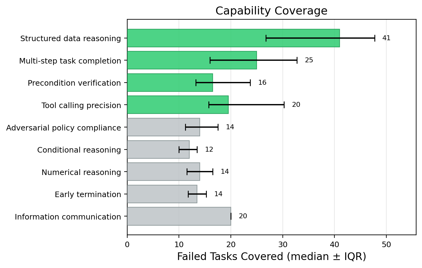
We analyze the capabilities identified by repeated contrastive analysis across 10 independent runs (Figure 3a). The pipeline consistently converges on a small set of lacking capabilities: structured data reasoning, multi-step task completion, and precondition verification are recovered in all 10 runs, while tool-calling precision appears in 8 of 10.

Beyond selection frequency, failure coverage is heavily concentrated within these specific capabilities (Figure 3b). Structured data reasoning accounts for the largest share of failed benchmark tasks, followed closely by multi-step task completion. This skewed distribution empirically validates our approach of explicitly isolating and targeting the lacking capabilities responsible for a significant proportion of failures, which maximizes data efficiency. More detailed analysis is provided in Appendix I.

(a) Scaling the number of capabilities (TRACE vs. GEPA).

(b) Scaling the number of rollouts.

Figure 4: Method scaling on $\tau^{2}$-Bench. (a) TRACE overall pass rate as the number of trained capabilities increases, compared to GEPA prompt optimization. (b) Pass rate as the number of rollouts increases for TRACE, GEPA, and GRPO on the target environment.

4.4 Method Scaling

Figure 4(a) shows how TRACE’s overall pass rate scales with the number of trained capabilities. In contrast, GEPA, which optimizes capability descriptions in the prompt, plateaus after 4 capabilities. Figure 4(b) illustrates how performance on $\tau^{2}$-Bench scales with the number of rollouts for TRACE, GEPA, and running GRPO on the target environment. TRACE demonstrates consistent, monotonic improvement, scaling from a base pass rate of 32.9% up to 48.2% at 5,120 rollouts. In contrast, GEPA plateaus early, reaching only 39.6%, while GRPO exhibits instability, dropping to 35.4% at 3,840 rollouts, and ultimately stalls at 37.8%. A consistent trend appears on ToolSandBox (Appendix B).

5 Conclusion

In this work, we propose TRACE, an end-to-end system for environment-specific agent self-improvement that automatically identifies lacking capabilities from the agent’s trajectories, synthesizes targeted training environments for each capability, trains capability-specific LoRA adapters via RL, and then trains a Mixture-of-Experts (MoE) model over the capability adapters. TRACE can be effectively applied across different environments, improving over the base agent by +15.3 points on $\tau^{2}$-Bench (customer service) and +15 points Pass@1 on SWE-bench Verified (software engineering), outperforming the strongest external baseline by +8.6 points and +9 points, respectively. Given the same number of rollouts, TRACE scales more efficiently than baselines, outperforming GRPO and GEPA by +10.4 and +8.6 points on $\tau^{2}$-Bench, respectively.

Appendix A GRPO Details

Given the family of synthetic environments $\{\mathcal{E}_{s}^{c}\}_{c\in\mathcal{C}^{*}}$ produced by the environment generation pipeline (§3.3), we train a separate low-rank adapter (Hu et al., 2021) $\Delta_{c}$ for each capability $c\in\mathcal{C}^{*}$ while keeping the base model $\pi_{\theta}$ frozen.

GRPO training. We train with Group Relative Policy Optimization, an on-policy reinforcement learning algorithm that avoids learning an explicit value function. For each capability $c$, the adapted policy $\pi_{\theta+\Delta_{c}}$ interacts with the corresponding synthetic environment $\mathcal{E}_{s}^{c}$. At each training iteration, the policy generates $G$ groups of rollouts. Within each group $g$, $K$ trajectories $\{\tau_{g,1},\dots,\tau_{g,K}\}$ are sampled from the same environment seed $z_{g}$, so that all $K$ rollouts begin from an identical initial state and differ only through stochastic decoding. Let $r_{g,k}=R_{\mathcal{E}_{s}^{c}}(x_{g},\tau_{g,k})$ denote the reward assigned by the programmatic verifier of $\mathcal{E}_{s}^{c}$, where $x_{g}=G_{\mathcal{E}_{s}^{c}}(z_{g})$. GRPO computes a group-relative normalized advantage for each trajectory,

$$\hat{A}_{g,k}=\frac{r_{g,k}-\bar{r}_{g}}{\sigma_{g}+\epsilon},\qquad\bar{r}_{g}=\frac{1}{K}\sum_{j=1}^{K}r_{g,j},\qquad\sigma_{g}=\sqrt{\frac{1}{K}\sum_{j=1}^{K}(r_{g,j}-\bar{r}_{g})^{2}},$$ (1)

where $\bar{r}_{g}$ and $\sigma_{g}$ are the within-group mean and standard deviation. This normalization makes the training signal invariant to reward scale across capabilities and synthetic environments. Because reward is assigned at the trajectory level, all action tokens in a rollout receive the same advantage. Groups in which all $K$ rollouts receive identical rewards are discarded, since they provide no learning signal.

The adapter parameters are updated using the clipped GRPO surrogate objective

$$\mathcal{L}_{\mathrm{GRPO}}=-\frac{1}{|\mathcal{B}|}\sum_{(g,k)\in\mathcal{B}}\frac{1}{T_{g,k}}\sum_{t=1}^{T_{g,k}}\min\!\Bigl(\rho_{t}\hat{A}_{g,k},\mathrm{clip}(\rho_{t},1-\epsilon,1+\epsilon)\hat{A}_{g,k}\Bigr),$$ (2)

where

$$\rho_{t}=\frac{\pi_{\theta+\Delta_{c}}(a_{t}\mid x,a_{<t})}{\pi_{\theta+\Delta_{c}}^{\mathrm{old}}(a_{t}\mid x,a_{<t})}$$

is the per-token importance ratio between the current and rollout policies, $a_{t}$ denotes the $t$-th token in the trajectory, $T_{g,k}$ is the number of tokens in trajectory $\tau_{g,k}$, $\mathcal{B}$ denotes the minibatch, and $\epsilon$ is the clipping threshold. As in PPO-style methods, clipping prevents excessively large policy updates when the estimated advantage is high.

On-policy rollout collection. At each iteration, we synchronize the current adapter $\Delta_{c}$ to a separate inference worker and collect rollouts on-policy from $\pi_{\theta+\Delta_{c}}$. The policy interacts with the task generator $G_{\mathcal{E}_{s}^{c}}$, receives observations, invokes tools, and continues until the episode terminates, after which the reward function $R_{\mathcal{E}_{s}^{c}}$ assigns the terminal reward. Because rollouts are collected on-policy, the importance ratio $\rho_{t}$ remains close to $1$ at the beginning of each update, which improves optimization stability.

Appendix B ToolSandbox Evaluation

We additionally evaluate TRACE on ToolSandBox (Lu et al., 2025) (129 base scenarios), a stateful, conversational tool-use benchmark. We report mean similarity, the average $[0,1]$ trajectory score from the benchmark’s milestone-based evaluator, and perfect rate, the fraction of scenarios scoring exactly $1.0$ (formal definitions in Appendix F). For TRACE, the two capabilities trained are permission error recovery and datetime reasoning (Appendix J). As in the main paper, all baselines are run under matched training budgets and evaluated with greedy decoding.

Table 3: Perfect Score (similarity $=1.0$) and Mean Similarity on ToolSandBox

Model	Perfect	Mean Sim.
Base	19/129	0.411
ADP	19/129	0.422
GRPO on Target	22/129	0.519
AWM	20/129	0.504
GEPA	22/129	0.520
Single Capability GRPO (Ours)	22/129	0.514
TRACE (Ours)	26 / 129	0.560

Table 3 summarizes the results. TRACE achieves a mean similarity of $0.560$ with $26$ perfect scores, improving over the base model by $+0.149$ mean similarity and $7$ additional perfect scores, and over the strongest external baseline by $+0.040$ mean similarity and $4$ additional perfect scores. A single adapter trained on one synthesized capability environment already reaches $0.514$, surpassing the general-purpose AWM ($0.504$) and ADP ($0.422$) baselines, while prompt optimization with GEPA reaches $0.520$. These trends mirror those on $\tau^{2}$-Bench and SWE-bench Verified: diagnosing and training the specific missing capabilities outperforms both general-purpose training data and prompt optimization.

Figure 5: Mean similarity on ToolSandBox as the number of rollouts is scaled. As on $\tau^{2}$-Bench, TRACE improves steadily to a $0.560$ mean similarity score, outperforming both GEPA ($0.520$) and GRPO ($0.519$).

Appendix C Capability Consolidation

Table 4: Single Model Consolidation Approaches on $\tau^{2}$-Bench

Approach	Airline (%)	Retail (%)	Overall (%)
Base	24.0	36.8	32.9
Single Capability GRPO	34.0	43.0	40.3
CORE-TSV	36.0	41.2	39.6
On Policy Distillation	28.0	42.1	37.8
SFT Synthetic	36.0	38.6	37.8
Multi Capability GRPO	38.0	42.1	40.9
TRACE	44.0	50.0	48.2

In Table 4, we compare TRACE MoE against alternatives to consolidate capabilities into one model. CORE-TSV merge (Panariello et al., 2025b; Ilharco et al., 2023b; Yadav et al., 2023a) combines independently trained, capability-specific adapters in a shared low-rank space using Core Space merging, task-vector composition, and TIES-style sign resolution. Multi-Capability GRPO trains a single LoRA adapter on a uniform mixture of all synthesized capability environments. SFT Synthetic trains a single LoRA adapter on successful trajectories collected from all the synthesized capability environments. On-Policy Distillation trains a LoRA teacher for each synthetic capability environment, then trains one student LoRA on a uniform mix by having the student generate on-policy rollouts and match the relevant teacher’s token-level distributions (Lu and Lab, 2025). All consolidation approaches are trained under matched budgets. Only Multi-Capability GRPO (40.9%) marginally outperforms the best single adapter (40.3%), whereas MoE significantly outperforms it.

Appendix D Parameter Counts

Table 5: Parameter counts for TRACE Model.

Component	Number of Parameters
Qwen3-30B-A3B backbone (frozen)	$\sim\!30.5$ B
Capability LoRA adapter (each)	$\sim\!1.6$ B
MoE gate (Linear $d{\to}|\mathcal{C}^{*}|$, one per block)	491,760

Table 5 breaks down the parameters of each TRACE component. The Qwen3-30B-A3B backbone ($\sim\!30.5$ B parameters) remains frozen throughout the entire pipeline. Each capability-specific LoRA adapter introduces $\sim\!1.6$ B trainable parameters (corresponding to $5.3\%$ of the backbone) and is optimized independently on its respective synthetic environment during the RL stage (§3.4). At the composition stage (§3.5), the backbone and all $|\mathcal{C}^{*}|$ capability adapters are frozen, and the only trainable parameters are the MoE gates: one linear map from the block’s hidden dimension $d$ to the $|\mathcal{C}^{*}|$ capability logits per adapted transformer block, totaling $491{,}760$ parameters across all blocks.

Although TRACE stores all $|\mathcal{C}^{*}|$ adapters, inference is sparse: at each token, the MoE gate selects the top-$k$ capabilities, so only $k$ of the adapters are active. In our experiments we find $k{=}1$ works well, holding the per-token active parameter count to the backbone’s active footprint plus a single adapter.

Appendix E Environment Generation Prompt

Appendix F Metrics Detail

The overall pass rate for $\tau^{2}$-Bench is defined as:

$$\mathrm{PassRate}_{\mathrm{overall}}=\frac{S_{\mathrm{Airline}}+S_{\mathrm{Retail}}}{N_{\mathrm{Airline}}+N_{\mathrm{Retail}}},$$

where $S_{\mathrm{Airline}}$ and $S_{\mathrm{Retail}}$ denote the numbers of solved tasks in the two domains, and $N_{\mathrm{Airline}}$ and $N_{\mathrm{Retail}}$ denote the corresponding numbers of benchmark tasks.

The Pass@1 for SWE-bench Verified is defined as:

$$\mathrm{Pass@1}=\frac{1}{N_{\mathrm{SWE}}}\sum_{i=1}^{N_{\mathrm{SWE}}}\mathbf{1}\!\left[\text{patch}_{i}\text{ resolves issue }i\right],$$

where the indicator is $1$ if and only if the single patch generated for instance $i$ applies cleanly and passes all of that instance’s held-out tests, and $N_{\mathrm{SWE}}=500$ is the number of SWE-bench Verified instances.

The mean similarity and the perfect score for ToolSandBox is defined as:

$$\mathrm{MeanSimilarity} =\frac{1}{N_{\mathrm{TS}}}\sum_{i=1}^{N_{\mathrm{TS}}}\mathrm{Sim}_{i},$$ (3)

$$\mathrm{PerfectRate} =\frac{1}{N_{\mathrm{TS}}}\sum_{i=1}^{N_{\mathrm{TS}}}\mathbf{1}\!\left[\mathrm{Sim}_{i}=1\right].$$ (4)

where $\mathrm{Sim}_{i}$ denotes the final ToolSandbox similarity score for trajectory $\tau_{i}$, and $N_{\mathrm{TS}}$ is the number of evaluated ToolSandbox scenarios.

Appendix G Results with Stochastic Decoding

The main paper uses greedy decoding (temperature $T=0$, seed $42$) for deterministic reproducibility, which yields a single sample per task. We re-ran all baselines and TRACE at temperature $0.7$ with $3$ seeds and report the mean $\pm$ 95% confidence interval (CI) in Tables 6 and 7. As shown in the tables, TRACE consistently outperforms all baselines on both benchmarks, with non-overlapping CIs.

Table 6: Pass rate on $\tau^{2}$-Bench under stochastic decoding (temperature $0.7$, $3$ seeds). We report mean $\pm$ 95% CI.

Approach	Airline (%)	Retail (%)	Overall (%)
Base	$21.3\pm 2.9$	$36.3\pm 2.5$	$32.1\pm 1.8$
GRPO	$30.7\pm 5.7$	$38.9\pm 3.3$	$36.4\pm 3.2$
GEPA	$36.7\pm 2.9$	$38.6\pm 2.2$	$38.0\pm 1.7$
TRACE	$\mathbf{44.0\pm 5.0}$	$\mathbf{47.1\pm 2.5}$	$\mathbf{46.1\pm 3.2}$

Table 7: Pass rate and mean similarity on ToolSandBox under stochastic decoding (temperature $0.7$, $3$ seeds). We report mean $\pm$ 95% CI.

Model	Pass Rate (%)	Mean Sim.
Base	$14.2\pm 2.2$	$0.40\pm 0.03$
GRPO	$16.3\pm 1.9$	$0.51\pm 0.02$
GEPA	$16.8\pm 1.1$	$0.52\pm 0.01$
TRACE	$\mathbf{21.2\pm 2.2}$	$\mathbf{0.56\pm 0.02}$

Appendix H Cross-Environment Transfer

We furthermore evaluate cross-environment transfer in Table 8. A model trained with TRACE or GRPO on $\tau^{2}$-Bench is evaluated on a second tool-calling benchmark, ToolSandBox, without re-training. The TRACE-trained agent still transfers more effectively than the GRPO-trained one ($+1$ perfect score and $+0.052$ mean similarity), indicating that TRACE’s targeted training yields capabilities that carry over to a new environment rather than merely overfitting to the training benchmark.

Table 8: Cross-environment transfer evaluated on ToolSandBox. Agents trained with GRPO or TRACE on $\tau^{2}$-Bench are evaluated on ToolSandBox without re-training; the bottom block reports in-domain ToolSandBox training for reference. We report perfect score (similarity $=1.0$) out of $129$ scenarios and mean similarity.

Method	Trained on	Perfect	Mean Sim.
Base	—	19/129	0.411
GRPO	$\tau^{2}$-Bench	19/129	0.430
TRACE	$\tau^{2}$-Bench	20/129	0.482
GRPO	ToolSandBox	22/129	0.519
TRACE	ToolSandBox	26/129	0.552

Appendix I Extended Capability Analysis

While the analysis agent consistently selects the top five capabilities (as discussed in Section 4.3), it frequently discards competing categories. Candidates such as conditional reasoning, numerical reasoning, early termination, and information communication appeared much less frequently across the 10 independent runs. This long-tail distribution confirms that the target benchmark’s failure modes are concentrated rather than uniform.

Additionally, we note that the coverage counts reported in Figure 3(b) are not mutually exclusive. A single failed benchmark trajectory often involves multiple missing capabilities—for example, an agent might fail to verify a precondition before executing a multi-step task. The contrastive analysis successfully disentangles these overlapping failures, allowing the framework to synthesize isolated micro-environments for each distinct deficit.

Appendix J Capability Details

J.1 Training Capabilities and Trajectory Examples

We identify four primary capability gaps through contrastive analysis of failed baseline trajectories on $\tau^{2}$-Bench. Each capability targets a distinct failure mode.

C1: Structured Data Reasoning. The agent fails to parse or cross-reference structured records returned by tools. Example: A user requests an economy flight departing after 11 AM. The search tool returns flights with nested price arrays per cabin class. The base model misreads which price corresponds to economy, computes the wrong total, and the booking fails with repeated payment errors.

C2: Tool Calling Precision. The agent identifies the correct tool but passes wrong arguments. Example: A user requests a refund to their original payment method (credit card). The agent retrieves the order (showing credit_card_3892 as payment) and the user profile (containing both credit_card_3892 and gift_card_1234). When calling return_delivered_order_items, it passes gift_card_1234 instead of the correct credit_card_3892.

C3: Multi-Step Task Completion. The agent completes the first sub-task of a compound request then stops. Example: A user asks to cancel two reservations and modify a third. The agent successfully cancels the first reservation, generates a closing statement ("If you need any further assistance…"), and never attempts the remaining two operations—entering a sycophancy loop with the user simulator until timeout.

C4: Precondition Verification. The agent executes state-changing actions without checking policy eligibility. Example: A user requests cancellation of a basic economy flight booked 14 days ago with no insurance. The policy requires at least one of: booked within 24 hours, airline-cancelled flight, business class, or covered insurance. None apply, but the agent calls cancel_reservation without checking any condition. The API does not enforce policy—the agent must independently verify eligibility.

J.2 ToolSandbox Training Capabilities and Trajectory Examples

We identify two primary capability gaps through analysis of base model trajectories on ToolSandbox:

C1: Permission Error Recovery. When a tool call returns a PermissionError due to a device setting conflict, the base model stops and reports the error to the user instead of resolving the underlying issue. Example: The user asks “Turn on wifi.” The agent calls set_wifi_status(on=True), which returns PermissionError: Wifi cannot be turned on in low battery mode. The base model halts—the conversation ends with only 2 messages. The correct behavior is to diagnose the blocker by calling get_low_battery_mode_status (returns True), disable it with set_low_battery_mode_status(on=False), retry the original set_wifi_status(on=True), and communicate success to the user.

C2: Datetime Reasoning. The base model skips the timestamp_to_datetime_info tool and instead attempts to mentally decode Unix timestamps, consistently hallucinating the wrong date. Example 1: The user asks “Remind me to buy chocolate milk tomorrow 5PM.” The agent calls get_current_timestamp (returns 1774511873), then directly calls datetime_info_to_timestamp(year=2026, month=3, day=25, …)—guessing the current date from the raw timestamp and getting the day wrong (March 25 instead of March 26), setting the reminder in the past. The correct behavior is to first call timestamp_to_datetime_info(1774511873) which returns the exact date {year: 2026, month: 3, day: 26, …}, then compute tomorrow as March 27. Example 2: The user asks “How many days till Christmas Day?” The base model calls search_holiday("Christmas Day", year=2023)—defaulting to a training-data year—and computes -823 days (past). The correct behavior is to first determine the current year via get_current_timestamp followed by timestamp_to_datetime_info, then search for the holiday in the correct year (2026), yielding 273 days.

Appendix K Synthetic Environment Example

K.1 Structured Data Reasoning ($\tau^{2}$-Bench)

K.2 Error Recovery (ToolSandBox)