MI-Pruner: Crossmodal Mutual Information-guided Token Pruner
for Efficient MLLMs

Abstract

For multimodal large language models (MLLMs), visual information is relatively sparse compared with text. As a result, research on visual pruning emerges for efficient inference. Current approaches typically measure token importance based on the attention scores in the visual encoder or in the LLM decoder, then select visual tokens with high attention scores while pruning others. In this paper, we pursue a different and more surgical approach. Instead of relying on mechanism-specific signals, we directly compute Mutual Information (MI) between visual and textual features themselves, prior to their interaction. This allows us to explicitly measure crossmodal dependency at the feature levels. Our MI-Pruner is simple, efficient and non-intrusive, requiring no access to internal attention maps or architectural modifications. Experimental results demonstrate that our approach outperforms previous attention-based pruning methods with minimal latency.

Figure 1: Pruning visualization on LLaVA1.5-7B with different budgets. Our MI-Pruner consistently identifies and preserves the queried regions, whereas other methods partially miss relevant information. Tokens from top to bottom: 64, 128, 256.

1 Introduction

“Tell the whole story from just one clue.” — A principle

Modern multimodal models have rapidly grown in scale and capability (Bai et al., 2025; Chen et al., 2024c; Liu et al., 2024b), but this progress comes with a substantial computational cost. In particular, the quadratic complexity of self-attention makes inference increasingly expensive as the number of tokens grows, especially for high-resolution visual inputs (Li et al., 2024). Therefore, token pruning has emerged as a critical mechanism for efficient inference, aiming to retain only the most informative tokens while discarding redundant ones (Ye et al., 2025; Cao et al., 2024). By reducing sequence length in the forward pass, the pruning not only alleviates computation and memory consumption, but also enables scalable deployment of large multimodal models in latency- and resource-constrained settings.

The token pruning task is grounded in information quantities (Iyer et al., 2021; Spadaro et al., 2023; Gao et al., 2020; Potkins et al., 2024), such as entropy and Mutual Information. Yet, most methods (Yang et al., 2025a; Zhao et al., 2025; Yin et al., 2025) merely consider the ”visual dilution” after shallow layers in the LLM decoder, and conduct pruning according to internal salience, e.g., attention scores. This design choice is not arbitrary, since studies on MLLM information flow (Zhang et al., 2025f, d) suggest a functional hierarchy across layers: shallow layers predominantly capture perceptual cues (the ”eye”), while deeper layers are responsible for high-level semantic reasoning and crossmodal fusion (the ”brain”). Consequently, attention in early decoder layers holds fine-grained perceptual saliency to be a reasonable proxy for identifying redundant tokens. Recent work (Zhang et al., 2025b; Yang et al., 2025a; Cai et al., 2025) points out that the entangled multimodal semantics in LLM bring noise into visual pruning, and proposes to leverage visual cues extracted by the vision encoder, at an even earlier stage before projection layers.

Despite the progress, several issues remain in attention-based pruning. (i) Crude manipulation with less interpretability: Attention scores don’t equal information importance due to the positional bias (Wen et al., 2025a), attention sinks (Xiao et al., 2024; Yang et al., 2025c) and multi-head diversity (Zhang et al., 2025d; Kang et al., 2025a). Several works (Darcet et al., 2024; Laurençon et al., 2024; Yan et al., 2025) indicate that attention maps have outliers incongruous with local semantics, and the multi-head average obliterates the head-specific roles (Yang et al., 2025c; Kang et al., 2025a). (ii) Implementation bottlenecks: LLM internal operations are incompatible with FlashAttention (Dao et al., 2022; Dao, 2024; Chen et al., 2024a), while extracting attention matrices from the encoder increases memory overhead, especially for high-resolution inputs. From a long-term perspective, prompt-adaptive pruning is desirable while not relying on the entangled cross-attention within LLMs. To address this, we move beyond heuristic attention collection and revisit the information-theoretic foundations of token importance. Instead of relying on attention salience in encoders or decoders, we propose to directly quantify token relevance through their Mutual Information. Built on this principle, we introduce MI-Pruner, a surgical token pruning approach in the projection space, enabling reliable and non-intrusive token pruning which preserves query-relevant information. As a model-agnostic method, it can be easily applied to a wide range of MLLMs following the Enc-MLP-Dec paradigm. Experiments across many benchmarks demonstrate that our method achieves state-of-the-art performance with minimal latency. Moreover, we present MI-Attention, a unified approach integrating Mutual Information and attention for flexible usage.

In summary, our contributions are:

• We introduce a principled framework for visual token pruning. By maximizing crossmodal Mutual Information in the projection space, MI-Pruner efficiently captures visual cues aligned with the textual query.

• As a model-agnostic module, MI-Pruner can be seamlessly integrated into various off-the-shelf MLLMs and is compatible with existing attention-based methods to further refine the token selection.

• Empirical results reveal that attention scores are not the only measure of semantic importance, establishing a new foundation for statistical analysis of black-box MLLMs.

2 Preliminaries

2.1 MLLM Architecture

The general architecture of MLLMs can be formulated as a vision encoder $\mathbf{E_{v}}$ with a projection module $f$, a tokenizer $\mathbf{E_{T}}$, and an LLM decoder. Given an image $I$ and a prompt $P$, the encoders $\mathbf{E_{V,T}}$ extract features into:

$$\mathcal{V} :=\{\mathbf{v}_{i}\}_{i=1}^{N_{V}}=f(\mathbf{E_{V}}(I))\in\mathbb{R}^{N_{V}\times d},\quad\mathbf{v}_{i}\in\mathbb{R}^{d},$$ (1)

$$\mathcal{T} :=\{\mathbf{t}_{j}\}_{j=1}^{N_{T}}=\mathbf{E_{T}}(P)\in\mathbb{R}^{N_{T}\times d},\quad\mathbf{t}_{j}\in\mathbb{R}^{d}.$$ (2)

The multimodal features are concatenated to input LLM:

$$\mathcal{X}:=\mathcal{V}\oplus\mathcal{T}\in\mathbb{R}^{(N_{V}+N_{T})\times d}.$$ (3)

We omit the system instructions for simplification. The LLM generates response tokens $\mathcal{Y}:=\{\mathbf{y}_{k}\}_{k=1}^{N_{G}}$ in an autoregressive manner:

$$p(\mathcal{Y}_{k}|\mathcal{X},\mathcal{Y}_{<k})=\mathrm{softmax(LLM}(\mathcal{X},\mathcal{Y}_{<k}))$$ (4)

2.2 Token Importance Measure

To assess token importance, methods based on visual cues (Zhang et al., 2025b; Yang et al., 2025a) typically employ a two-step pruning strategy: (i) aggregate attention scores from [CLS] or other image tokens from $\mathcal{V}$ as $\mathrm{Attn}_{i}$, to determine the initial pruning budget; (ii) recycle from remaining tokens $\mathcal{V}_{\mathrm{re}}$ by their similarity $S_{i}$. Assuming $c$ as the [CLS] index of an averaged attention matrix $\mathbf{A}\in\mathbb{R}^{N_{V}\times N_{V}}$ and $\tilde{\mathbf{v}}_{i}\in\mathbb{R}^{d}$ as the normalized visual embeddings before projection, the two-step importance measures are formulated as:

$$\mathrm{Attn}_{i} =\mathbf{A}_{ci}~\text{or}~\sum_{j\neq i,j\in\mathcal{V}}\mathbf{A}_{ji},$$ (5)

$$S_{i} =\sum_{j\neq i,j\in\mathcal{V}_{\mathrm{re}}}(\tilde{\mathbf{v}}_{i}^{\top}\tilde{\mathbf{v}}_{j}).$$ (6)

Then the selected visual tokens $\mathcal{V}_{\mathrm{keep}}$ go through projection to be concatenated with $\mathcal{T}$.

2.3 Information Theory

In this work, we study token pruning in MLLMs, aiming to identify and retain the most informative vision tokens. Information theory provides a rigorous mathematical framework for quantifying information transmission and representation. Within this framework, Mutual Information (MI) emerges as a natural metric for measuring the statistical dependence between tokens. Consequently, maximizing MI offers a principled objective for identifying tokens that encapsulate shared and semantically aligned information.

Definition 2.1 (Mutual Information (Kraskov et al., 2004; Gray, 2011)).

The Mutual Information $\mathrm{MI}(X;Y)$ measures the gap between entropy $H(X)$ and conditional entropy $H(X|Y)$ (see definition in App. A.1), which quantifies the uncertainty reduction of a random variable $X$ given the knowledge of another random variable $Y$:

$$\operatorname{MI}(X;Y) =H(X)-H(X\mid Y)$$ (7)

$$=\sum_{x\in\mathcal{X},\,y\in\mathcal{Y}}p(x,y)\underbrace{\log\frac{p(x\mid y)}{p(x)}}_{\operatorname{PMI}(x;y)}.$$ (8)

$\operatorname{MI}(X;Y)$ can be interpreted as the weighted average of pointwise Mutual Information $\operatorname{PMI}(x,y)$ under the joint distribution $p(x,y)$. Replacing $x,y$ with embeddings $\mathbf{v}_{i},\mathbf{t}_{j}$ establishes a link to multimodal token relevance. In general, maximizing MI is computationally intractable. However, under the assumption of conditional independence (the components of $X$ are independent given $Y$), it becomes a cardinality-constrained monotone submodular maximization problem (Krause et al., 2008). This is a well-studied problem with a known approximation guarantee of $1-1/e$. An important property of submodular functions is the marginal gain.

Definition 2.2 (Marginal Gain (Fujishige, 2005)).

Let $\mathcal{X}$ be a ground set, and let $f:2^{\mathcal{X}}\to\mathbb{R}$ be a set function. The marginal gain of adding an element $i\in\mathcal{X}\setminus\mathcal{A}$ to a selected set $\mathcal{A}\subseteq\mathcal{X}$ is defined as:

$$\Delta f(i|\mathcal{A})=f(\mathcal{A}\cup\{i\})-f(\mathcal{A}).$$ (9)

Definition 2.3 (Submodularity and Diminishing Returns (Fujishige, 2005)).

A function $f$ is submodular if and only if for all $\mathcal{A}\subseteq\mathcal{B}\subseteq\mathcal{X}$ and $i\in\mathcal{X}\setminus\mathcal{B}$:

$$\Delta f(i|\mathcal{A}) \geq\Delta f(i|\mathcal{B}).$$ (10)

Then, we link the monotonicity with MI-guided visual selection. Let $\mathcal{V}_{\mathrm{S}}\subseteq\mathcal{V}$ be a selected set belonging to a ground set of variables, and let $\mathcal{T}$ be a targeted set of variables, we define Mutual Information as a set function:

$$f(\mathcal{V}_{\mathrm{S}}) =\mathrm{MI}(\mathcal{V}_{\mathrm{S}};\mathcal{T}).$$ (11)

Following Eqn. (9), the marginal gain of adding a new $\mathbf{v}_{i}$ into $\mathcal{V}_{\mathrm{S}}$ is expressed as:

$$\Delta f(\mathbf{v}_{i}\mid\mathcal{V}_{\mathrm{S}}) =\mathrm{MI}(\mathcal{V}_{\mathrm{S}}\cup\{\mathbf{v}_{i}\};\mathcal{T})-\mathrm{MI}(\mathcal{V}_{\mathrm{S}};\mathcal{T})$$ (12)

$$=\mathrm{MI}(\mathbf{v}_{i};\mathcal{T}\mid\mathcal{V}_{\mathrm{S}}).$$ (13)

The definition of conditional MI is given in Def. A.3 (App. A.1), and the proof from Eqn. (12) to (13) is in App. A.2.

The cardinality-constrained monotone submodular maximization problem is typically addressed by a greedy search strategy, which selects elements that maximize the marginal gain at each step (Nemhauser et al., 1978):

$$\mathbf{v}_{i} =\arg\max_{\mathbf{v}_{i}\in\mathcal{V}\setminus\mathcal{V}_{\mathrm{S}}}\Delta f(\mathbf{v}_{i}|\mathcal{V}_{\mathrm{S}}).$$ (14)

The greedy search holds a complexity of $\mathcal{O}(N_{V}N_{\mathrm{keep}})$. In practice, greedy search is a common optimization strategy in token pruning (Alvar et al., 2025; Zhang et al., 2025c). In the sequel, we will develop a pruning strategy with even lower complexity.

3 Methods

Figure 2: Overview. Previous methods prune tokens by attention scores from vision encoder or LLM decoder. Our MI-Pruner calculates Mutual Information between visual and textual embeddings in the projection space, achieving optimal performance with minimal latency.

3.1 Visual Pruning

Compared to text, the visual information is inherently sparser (Tang et al., 2025; Chen et al., 2024b), while the image tokens usually consume $10\sim 100\times$ tokens than their textual counterparts. The reasons are two-fold: (i) Intrinsic visual redundancy: A vast majority of image patches consist of uninformative backgrounds or repetitive textures. (ii) Functional asymmetry in MLLMs: In multimodal contexts, text typically serves as a concentrated prompt to trigger specific visual reasoning, whereas the raw visual input is exhaustive. As illustrated in Fig. 1, repetitive regions—such as stretches of beach, flooring, or walls—are ubiquitous in visual data. Processing these redundant patches provides diminishing returns in representational gain while significantly inducing computational latency during the forward pass. Furthermore, the relative region regarding a concrete query takes even less portion, e.g., a shirt.

Despite the progress on visual pruning methods (Farina et al., 2024; Jeddi et al., 2025; Wang et al., 2023), most of them were constrained by the attention collection, which introduces significant latency due to additional storage requirements. Furthermore, the divergence across multiple heads and the attention sink phenomenon become a performance bottleneck. In this work, we circumvent these pitfalls by proposing a surgical approach based on Mutual Information in the projection space (Fig. 2).

3.2 MI-Pruner

After the projection layer, we extract visual embeddings $\mathcal{V}=\{\mathbf{v}_{i}\}_{i=1}^{N_{V}}$, and textual embeddings $\mathcal{T}=\{\mathbf{t}_{j}\}_{j=1}^{N_{T}}$, where $\mathbf{v}_{i},\mathbf{t}_{j}\in\mathbb{R}^{d}$. Our objective is to prune visual patches that are weakly correlated with the textual semantics yet highly redundant among selected patches. We denote $\tilde{x}$ as the normalized $x$. To save space, we adopt a unified notation: $\mathrm{s}\in\{\text{cross},\text{self}\},\mathbf{x}\in\{\mathbf{t},\mathbf{v}\},N\in\{N_{T},N_{V}\}$.

Normalization and similarity computation. We first normalize embeddings $\mathcal{V},\mathcal{T}$ onto a unit hypersphere, yielding $\tilde{\mathcal{V}},\tilde{\mathcal{T}}$. Based on Boltzmann distributions, we compute similarity matrices for vision-text ($\bm{\rho}_{ij}^{\mathrm{cross}}$) and vision-vision ($\bm{\rho}_{ij}^{\mathrm{self}}$) interactions:

$$\bm{\rho}_{ij}^{\mathrm{cross}}=\frac{\tilde{\mathbf{v}}_{i}^{\top}\tilde{\mathbf{t}}_{j}}{\tau},\quad\bm{\rho}_{ij}^{\mathrm{self}}=\frac{\tilde{\mathbf{v}}_{i}^{\top}\tilde{\mathbf{v}}_{j}}{\tau}.$$ (15)

The temperature $\tau$ controls the sharpness of the distribution, typically in 0.01$\sim$0.1. For simplicity, we adopt a shared $\tau$ for both matrices, though it’s not mandatory. Treating these similarity scores $\{\bm{\rho}_{ij}^{\mathrm{s}}\}_{j=1}^{N}$ as logits, we define the energy-based crossmodal and internal conditional distribution.

Conditional distribution. Applying a softmax operation along the second dimension, we obtain conditional probabilities $p(\tilde{\mathbf{t}}_{j}\mid\tilde{\mathbf{v}}_{i}),~p(\tilde{\mathbf{v}}_{j}\mid\tilde{\mathbf{v}}_{i})$ in a unified formula:

$$p(\tilde{\mathbf{x}}_{j}\mid\tilde{\mathbf{v}}_{i})=\operatorname{softmax}_{j}(\bm{\rho}_{ij}^{\mathrm{s}})=\frac{\exp(\bm{\rho}_{ij}^{\mathrm{s}})}{\sum_{k=1}^{N}\exp(\bm{\rho}_{ik}^{\mathrm{s}})}.$$ (16)

It quantifies the semantic alignment between $(\mathbf{v}_{i},\mathbf{t}_{j})$ and the structural diversity among $(\mathbf{v}_{i},\mathbf{v}_{j})$, as illustrated by the row operation in Fig. 3.

Marginal distribution. For the prior probability, we assume $p(\tilde{\mathbf{v}}_{j})=\frac{1}{N_{V}}$, where visual embeddings occur with equal probabilities to avoid spatial bias.

According to the law of total probability, the marginal distribution of text embeddings is expressed as:

$$p(\tilde{\mathbf{t}}_{j})=\frac{1}{N_{V}}\sum_{i=1}^{N_{V}}p(\tilde{\mathbf{t}}_{j}\mid\tilde{\mathbf{v}}_{i}),$$ (17)

as illustrated by the column operation in Fig. 3. See more details in App. A.4.

Pointwise Mutual Information. We adopt the Pointwise Mutual Information (PMI) to measure the token-level relevancy between embeddings:

$$\text{PMI}(\tilde{\mathbf{v}}_{i};\tilde{\mathbf{x}}_{j})=\log\frac{p(\tilde{\mathbf{x}}_{j}\mid\tilde{\mathbf{v}}_{i})}{p(\tilde{\mathbf{x}}_{j})}.$$ (18)

Specifically, $\text{PMI}(\tilde{\mathbf{v}}_{i};\tilde{\mathbf{t}}_{j})$ quantifies the crossmodal semantic alignment, while $\text{PMI}(\tilde{\mathbf{v}}_{i};\tilde{\mathbf{v}}_{j})$ captures the intra-modal redundancy; both are measured at the token level.

Figure 3: A toy model of MI-based pruning. We construct similarity matrices to get conditional probability and marginal probability, then calculate crossmodal PMI (top) and internal PMI (bottom). All [vis] tokens are flattened for illustration.

Table 1: Performance comparison of different pruning methods on LLaVA1.5-7B. Methods before - - - are attention-based. We use color to distinguish best and second best.

Methods	GQA	SQA	TextVQA	MMVet	MMEP	POPE	PF1	PYes
LLaVA1.5-7B	61.97	66.80	59.09	$30.46_{\pm 7.58}$	1509.13	85.18	0.86	0.56
lightgray    keep 64
FastV (Chen et al., 2024a)	50.80	51.10	47.80	24.99±7.01	1019.60	48.50	0.48	0.35
SparseVLM (Zhang et al., 2025e)	52.70	62.20	51.80	23.04±7.88	1221.10	75.45	0.75	0.37
VisionZip (Yang et al., 2025a)	55.10	69.00	55.50	31.04±7.08	1365.60	77.34	0.76	0.37
VisPruner (Zhang et al., 2025b)	55.40	69.10	55.80	32.09±7.11	1369.90	82.61	0.80	0.38
DART (Wen et al., 2025b)	55.90	68.86	54.40	26.01±6.78	1273.30	73.90	0.73	0.33
Random	55.45	67.34	49.54	23.60±6.91	1274.27	79.82	0.76	0.34
Similarity	54.63	68.47	50.30	24.04±6.88	1286.66	84.24	0.83	0.42
MI-Attention	57.01	69.20	55.90	31.16±8.33	1428.03	85.04	0.84	0.41
MI-Pruner	56.88	69.81	54.91	28.12±7.77	1381.35	84.91	0.83	0.43
lightgray    keep 32
FastV (Chen et al., 2024a)	41.50	42.60	42.50	20.55±7.34	884.60	33.50	0.33	0.34
SparseVLM (Zhang et al., 2025e)	48.30	57.30	46.10	18.81±7.05	1046.70	68.90	0.68	0.36
VisionZip (Yang et al., 2025a)	51.80	68.80	53.10	25.43±7.65	1247.40	68.92	0.68	0.37
VisPruner (Zhang et al., 2025b)	52.20	69.20	53.90	28.77±7.55	1271.00	77.83	0.73	0.32
DART (Wen et al., 2025b)	52.77	68.76	52.20	24.91±7.23	1273.30	69.13	0.69	0.31
Random	52.58	67.33	47.20	21.72±6.34	1176.85	73.23	0.66	0.30
Similarity	51.46	67.48	47.78	20.05±6.41	1141.68	80.07	0.78	0.42
MI-Attention	54.19	69.11	54.07	28.91±7.85	1344.16	82.81	0.81	0.39
MI-Pruner	55.78	69.26	52.63	24.46±7.77	1307.72	83.18	0.81	0.41

Maximal aggregation. For each $\tilde{\mathbf{v}}_{i}$, we aggregate the maximal PMI over text tokens $\tilde{\mathcal{T}}$ and over selected vision tokens $\tilde{\mathcal{V}}_{\mathrm{S}}$ as the crossmodal and internal relevance scores:

$$S_{i}^{\mathrm{cross}} =\max_{\tilde{\mathbf{t}}_{j}\in\tilde{\mathcal{T}}}{\mathrm{PMI}(\tilde{\mathbf{v}}_{i};\tilde{\mathbf{t}}_{j})},$$ (19)

$$S_{i}^{\mathrm{self}} =\max_{\tilde{\mathbf{v}}_{j}\in\tilde{\mathcal{V}}_{\mathrm{S}}}{\mathrm{PMI}(\tilde{\mathbf{v}}_{i};\tilde{\mathbf{v}}_{j})}.$$ (20)

The max aggregation forces $S_{i}^{\mathrm{s}}$ to capture the strongest crossmodal relevance (”pivot word”) and intra-modal redundancy (”pivot patch”), leading to consistently better performance than the global average. See justification in App. A.3.

Global aggregation. Another way is to the full MI formulation, i.e., averaging over all text tokens or selected image tokens (”consensus”), interpreted as global aggregation:

$$S_{i}^{\mathrm{s}} =\sum_{j=1}^{N_{X}}\underbrace{p(\tilde{\mathbf{v}}_{i};\tilde{\mathbf{x}}_{j})}_{p(\tilde{\mathbf{x}}_{j}\mid\tilde{\mathbf{v}}_{i})}\cdot{\mathrm{PMI}(\tilde{\mathbf{v}}_{i};\tilde{\mathbf{x}}_{j})}.$$ (21)

Empirical comparisons of the two aggregation strategies are presented in Sec. 4.4.

Greedy search. For greedy search, we define a scoring function $S_{i}$ as the marginal gain of adding $\mathbf{v}_{i}$, where $\lambda$ balances the relevance and redundancy:

$$S_{i}=\lambda S_{i}^{\mathrm{cross}}-(1-\lambda)\cdot S_{i}^{\mathrm{self}}$$ (22)

$$=\lambda\cdot\underbrace{\max_{\tilde{\mathbf{t}}_{j}\in\tilde{\mathcal{T}}}{\mathrm{PMI}(\tilde{\mathbf{v}}_{i};\tilde{\mathbf{t}}_{j})}}_{\text{relevance}\rightarrow\text{sorting}}-(1-\lambda)\underbrace{\max_{\tilde{\mathbf{v}_{j}}\in\tilde{\mathcal{V}}_{\mathrm{S}}}{\mathrm{PMI}(\tilde{\mathbf{v}}_{i};\tilde{\mathbf{v}}_{j})}}_{\text{redundancy}\rightarrow\text{greedy}}.$$ (23)

$\lambda=1$ considers only crossmodal relevance towards user prompts, and $\lambda=0$ measures only internal redundancy. According to the budget $N_{\mathrm{keep}}$, we conduct a greedy search to find $\mathbf{v}^{\star}$ that maximizes the marginal gain at each step:

$$\mathbf{v}^{\star} =\arg\max_{\mathbf{v}_{i}\in\mathcal{V}\setminus\mathcal{V}_{\mathrm{S}}}S_{i}.$$ (24)

Algorithm 1 MI-Pruner

1: Input: Visual and textual embeddings $\mathcal{V}=\{\mathbf{v}_{i}\}_{i=1}^{N_{V}}$, $\mathcal{T}=\{\mathbf{t}_{j}\}_{j=1}^{N_{T}}$, temperature $\tau$, budget $N_{\mathrm{keep}}$

2: Output: The selected visual subset $\mathcal{V}_{\mathrm{keep}}$

3: // Similarity matrices

4: $\tilde{\mathbf{v}}_{i}\leftarrow\mathbf{v}_{i}/\lVert\mathbf{v}_{i}\rVert,\tilde{\mathbf{t}}_{j}\leftarrow\mathbf{t}_{j}/\lVert\mathbf{t}_{j}\rVert$

5: $\bm{\rho}^{\mathrm{cross}}_{ij}\leftarrow\tilde{\mathbf{v}}_{i}^{\top}\tilde{\mathbf{t}}_{j}/\tau,\bm{\rho}^{\mathrm{self}}_{ij}\leftarrow\tilde{\mathbf{v}}_{i}^{\top}\tilde{\mathbf{v}}_{j}/\tau$

6: // Derive distributions

7: 

$p(\tilde{\mathbf{t}}_{j}|\tilde{\mathbf{v}}_{i})\leftarrow\text{softmax}_{j}(\bm{\rho}^{\mathrm{cross}}_{ij}),\ p(\tilde{\mathbf{v}}_{j}|\tilde{\mathbf{v}}_{i})\leftarrow\text{softmax}_{j}(\bm{\rho}^{\mathrm{self}}_{ij})$

8: $p(\tilde{\mathbf{v}}_{j})\leftarrow\frac{1}{N_{V}},p(\tilde{\mathbf{t}}_{j})\leftarrow\frac{1}{N_{V}}\sum_{i=1}^{N_{V}}p(\tilde{\mathbf{t}}_{j}\mid\tilde{\mathbf{v}}_{i})$

9: // Pointwise Mutual Information (PMI)

10: 

$\mathrm{PMI}(\tilde{\mathbf{v}}_{i};\tilde{\mathbf{t}}_{j})\leftarrow\log\frac{p(\tilde{\mathbf{t}}_{j}\mid\tilde{\mathbf{v}}_{i})}{p(\tilde{\mathbf{t}}_{j})},\mathrm{PMI}(\tilde{\mathbf{v}}_{i};\tilde{\mathbf{v}}_{j})\leftarrow\log\frac{p(\tilde{\mathbf{v}}_{j}\mid\tilde{\mathbf{v}}_{i})}{p(\tilde{\mathbf{v}}_{j})}$

11: // Greedy selection

12: while $|\mathcal{V}_{\mathrm{S}}|<N_{\mathrm{keep}}$ do

13:  for each $\mathbf{v}_{i}\in\mathcal{V}\setminus\mathcal{V}_{\mathrm{S}}$ do

14:   $S_{i}^{\mathrm{cross}}\leftarrow\max_{\tilde{\mathbf{t}}_{j}\in\tilde{\mathcal{T}}}{\mathrm{PMI}(\tilde{\mathbf{v}}_{i};\tilde{\mathbf{t}}_{j})}$

15:   $S_{i}^{\mathrm{self}}\leftarrow\max_{\tilde{\mathbf{v}}_{j}\in\tilde{\mathcal{V}}_{\mathrm{S}}}{\mathrm{PMI}(\tilde{\mathbf{v}}_{i};\tilde{\mathbf{v}}_{j})}$

16:   $S_{i}\leftarrow\lambda S_{i}^{\mathrm{cross}}-(1-\lambda)S_{i}^{\mathrm{self}}$

17:  end for

18:  $\mathbf{v}^{\star}\leftarrow\arg\max_{\mathbf{v}_{i}}S_{i},\text{and}~\mathcal{V}_{\mathrm{S}}\leftarrow\mathcal{V}_{\mathrm{S}}\cup\{\mathbf{v}^{\star}\}$

19: end while

20: $\mathcal{V}_{\mathrm{keep}}\leftarrow\mathcal{V}_{\mathrm{S}}$

21: return $\mathcal{V}_{\mathrm{keep}}$

3.3 Efficient Inference

Recall Sec. 2.1, MI-Pruner prunes vision tokens to a smaller set $\mathcal{V}_{\mathrm{keep}}$. In the projection space, Eqn. (3) is updated to:

$$\mathcal{X} =\mathcal{V}_{\mathrm{keep}}\oplus\mathcal{T}\in\mathbb{R}^{(N_{\mathrm{keep}}+N_{T})\times d},~N_{\mathrm{keep}}<N_{V}.$$ (25)

Since MI-Pruner doesn’t require attention collection or interaction of LLM, the scoring calculation is very efficient with minimal latency, and the subset selection problem becomes modular instead of just submodular. Our selection has a complexity of $\mathcal{O}(N_{V}+N_{\mathrm{keep}}\log N_{V})$, while the classic greedy search holds $\mathcal{O}(N_{V}N_{\mathrm{keep}})$. We expect that in settings of interest $N_{\mathrm{keep}}\log N_{V}<N_{V}$, implying an overall complexity of $\mathcal{O}(N_{V})$. See Algorithm 1 for our full pipeline. Then, we empirically verify that this faster inference framework results in comparable or better performance to SOTA baselines.

4 Experiments

4.1 Experiments Setup

Settings.

We adopt $\lambda=0.5$ for open-ended QA datasets, involving GQA (Hudson and Manning, 2019) and MMVet (Yu et al., 2023), and $\lambda=1$ for broader closed-form-type datasets, including SQA (Lu et al., 2022) (mutiple-choice), TextVQA (Singh et al., 2019) (reference answer provided), MME_P (Fu et al., 2025) (Yes/No) and POPE (Li et al., 2025) (Yes/No). The inference and evaluation follow the default settings and metrics. Specifically, we conduct bootstrapping for MMVet since it includes only 218 samples, and report F1 score (P_F1) and Yes-rate (P_Yes) for POPE as fine-grained measures. The MLLMs include LLaVA1.5-7B (Liu et al., 2024a), Qwen2VL (Wang et al., 2024) and latest Qwen3VL (Bai et al., 2025), all in greedy sampling and SDPA attention, more details in App. B.3. For generalization, we also apply our method to Video-LLaVA-7B (Lin et al., 2024) with $\lambda=0.5$ and test on TGIF-QA (Jang et al., 2017), MSVD-QA (Xu et al., 2017) and MSRVTT-QA (Xu et al., 2017) datasets. All experiments are conducted on a single NVIDIA A100 GPU.

Table 2: Performance comparison of different pruning methods on Qwen3VL-2B and -8B. ”Attention” refers to the sum of attention scores from other image tokens. MI-Pruner and MI-Attention achieve SOTA performance for both scales.

Methods	GQA	MMEP	POPE	PF1	PYes	Methods	GQA	MMEP	POPE	PF1	PYes
Qwen3VL-2B	59.55	1494.98	89.89	0.90	0.47	Qwen3VL-8B	61.53	1730.47	88.84	0.88	0.44
lightgray    keep 50%
Random	49.96	1438.19	88.76	0.88	0.46	Random	53.02	1422.31	88.25	0.87	0.43
Similarity	50.87	1454.34	89.26	0.89	0.48	Similarity	53.17	1461.25	88.95	0.88	0.45
Attention	50.09	1462.74	89.54	0.89	0.47	Attention	52.93	1462.84	88.85	0.88	0.44
MI-Pruner	51.30	1478.26	89.78	0.90	0.48	MI-Pruner	53.48	1493.04	89.22	0.89	0.45
MI-Attention	51.11	1493.20	89.73	0.89	0.48	MI-Attention	53.23	1482.10	89.00	0.88	0.44
lightgray    keep 25%
Random	47.15	1398.52	85.59	0.85	0.42	Random	49.47	1256.18	85.64	0.84	0.41
Similarity	48.43	1372.50	88.28	0.88	0.47	Similarity	50.61	1338.28	87.98	0.88	0.45
Attention	46.59	1158.90	86.39	0.85	0.41	Attention	49.00	1293.91	87.74	0.87	0.43
MI-Pruner	49.63	1447.14	89.51	0.89	0.48	MI-Pruner	51.42	1369.58	88.82	0.88	0.45
MI-Attention	48.53	1459.36	89.38	0.89	0.46	MI-Attention	50.72	1415.71	88.82	0.88	0.44

Comparison methods.

Our comparison involves the baseline with full tokens, attention-based and non-attention-based methods. For LLaVA1.5, we compare with (i) attention-based methods FastV (Chen et al., 2024a), SparseVLM (Zhang et al., 2025e), VisionZip (Yang et al., 2025a) and VisPruner (Zhang et al., 2025b), and (ii) non-attention-based methods DART (Wen et al., 2025b), random and similarity. ”Random” denotes averaging three independent runs with randomly selected tokens, and ”Similarity” refers to cosine similarity between V/T tokens (Eqn. (15)). As a variation, MI-Attention combines attention from the vision encoder (round-1) and MI-guided pruning (round-2). Since existing methods haven’t released codes on Qwen3VL, we establish a general ”Attention” baseline from VisionZip.

4.2 Main Results

LLaVA1.5.

Following the well-established benchmark in (Yang et al., 2025a; Zhang et al., 2025b), we report the pruning effects on LLaVA1.5-7B in Tab. 3.2. As observed, MI-Pruner and MI-Attention achieve SOTA performance among listed benchmarks. Specifically, other pruning methods significantly reduce the proportion of “Yes” responses to around 0.35, likely due to mistakenly pruning image tokens corresponding to the queried objects. In contrast, our method better preserves queried information in image tokens and maintains a more balanced Yes/No distribution. Surprisingly, not all pruning methods outperform ”Random” (Wang et al., 2025b; Wen et al., 2025b, a), underscoring the necessity of a solid theoretical grounding. In Fig. 1, we visualize the pruning effects of representative methods working in the projection space (ours), LLM (SparseVLM) and the vision encoder (VisPruner) respectively. The visualization shows that MI-Pruner consistently catches the queried region. Notably, our approach does not rely on collecting attention maps; this non-intrusive characteristic makes it more suitable for practical deployment.

Figure 4: Performance on Qwen2VL series (GQA).

(a) Qwen3VL-2B

(b) Qwen3VL-8B

Figure 5: Pruning visualization on Qwen3VL series. Our method retains the semantic-relative patches regarding prompts adaptively.

Qwen2VL and Qwen3VL series.

Despite the model-agnostic nature, we further evaluate our method on models with dynamic resolutions, both of instruction-tuned versions. For Qwen2VL series, we show performance on different generations ”-2VL” and ”-2.5VL” in Fig. 4. The visual cues in VisionZip depend on specific vision encoders, which limit its generalization capacity. In comparison, our method outperforms both diversity-based DART and attention-based VisionZip and FastV. For the latest Qwen3VL series, we illustrate two scales ”-2B” and ”-8B” in Tab. 4.1, where ”Attention” is implemented as the attention sum-up from other image tokens, to avoid the specific design of [CLS] or hyperparameters of existing methods (Yang et al., 2025a; Zhang et al., 2025b). Meanwhile, the visualization of pruning effects can be found in Fig. 5. By design, high-attention tokens produced by the vision encoder are biased toward generic salient features, such as faces or logos, which are pivotal for classification. However, such prompt-agnostic pruning exhibits reduced robustness when the query lies in non-salient or fine-grained regions that fall outside these pre-defined regions of interest. For instance, the ”Attention” method keeps the facial landmark in Fig. 4(a) while pruning the queried cars. The scattered patches among the swimmer and the swimming pool in Fig. 4(b) increase the difficulty of multimodal reasoning. In comparison, MI-Pruner provides semantically complete patches aligned with the query.

Efficiency analysis.

The MI derivative exhibits a complexity of $\mathcal{O}(N_{V}\cdot\max(N_{T},N_{\mathrm{keep}}))$, yet this overhead becomes $\mathcal{O}(N_{V}N_{T})$ for crossmodal priority ($\lambda=1$). Later, our selection complexity is $\mathcal{O}(N_{V}+N_{\mathrm{keep}}\log N_{V})$ due to the independence assumption. We report the GPU memory and latency in Tab. 3. Since SparseVLM operates in LLMs, its efficiency benefits are suboptimal. Despite the early stage in vision encoder, VisPruner is still held back by its attention collection. As a diversity-based method, CDPruner compromises the efficiency due to MAP inference. Despite a slight latency increase when intra-model redundancy is considered ($\lambda\neq 1$), MI-Pruner delivers the best inference efficiency under both configurations.

Table 3: Efficiency comparison on POPE (LLaVA1.5-7B).

Methods	Mem (GB)	Latency (ms)	Mem (GB)	Latency (ms)
lightgray	keep 128		keep 64
SparseVLM	18.08	96.36±0.35	18.11	93.67±0.31
VisPruner	14.35	92.04±0.44	14.35	89.48±0.32
CDPruner	14.73	111.12±0.65	14.65	91.41±0.41
DART	14.05	92.62±0.39	13.96	88.41±0.37
MI-Prunerλ=1	14.01	82.08±0.32	13.93	77.06±0.36
MI-Prunerλ=0.5	14.01	98.92±0.40	13.93	84.95±0.34

Table 4: Video-QA performance on Video-LLaVA-7B.

Methods	TGIF		MSVD		MSRVTT
	Acc	Score	Acc	Score	Acc	Score
Video-LLaVA	18.90	2.54	72.00	3.95	57.50	3.50
lightgray    keep 227
FastV	14.30	2.42	68.90	3.90	53.00	3.40
VisPruner	15.90	2.41	69.30	3.92	55.60	3.45
MI-Pruner	15.70	2.44	70.60	3.94	56.40	3.46
lightgray    keep 114
FastV	10.60	2.29	64.10	3.78	52.40	3.39
VisPruner	14.10	2.35	65.40	3.79	54.10	3.41
MI-Pruner	13.10	2.40	69.90	3.92	55.30	3.49

4.3 Video Understanding Results

Following previous work (Yang et al., 2025a), we report our video-QA results on Video-LLaVA (Lin et al., 2024), which includes 8 frames with $256\times 8=2048$ visual tokens. As shown in Tab. 4.2, MI-Pruner achieves average 93.19% accuracy across three datasets with merely 114 visual tokens (5.57% retained).

4.4 Ablation Study

Aggregation strategies.

We adopt max PMI (Eqn. (19)-(20)) as the MI proxy. In Fig. 5(a), we compare max with average aggregation. Empirically, the mean value among all text embeddings exhibits less distinguishing sensitivity to the queried object.

Balancing factor $\lambda$.

Fig. 5(b) reveals a dichotomy between open-ended (e.g., GQA) and closed-form datasets (e.g., SQA). The highest metrics are annotated for distinguishing. The prompts query about high-level semantics in open-ended questions (”What is …”), where a non-zero $\lambda$ is essential to prevent selecting highly similar visual elements. While for the multiple-choice dataset SQA, setting $\lambda=1$ consistently yields the best performance, as the prompt explicitly encodes the ground-truth cue in choices.

Temperature $\tau$.

The temperature $\tau$ is used to sharpen the similarity scores, especially for open-ended questions. We evaluate 3 groups of $\tau$ in Tab. 5 with 64 and 32 retained tokens, where $\tau=0.1$ yields the best performance.

(a) Aggregation

(b) Factor $\lambda$

Figure 6: Ablation study on scoring functions (LLaVA1.5-7B).

Table 5: Ablation study on temperature (LLaVA1.5-7B).

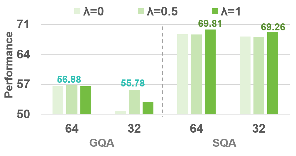
$\tau$	GQA64	GQA32	SQA64	SQA32
0.01	55.26	55.39	69.06	69.02
0.1	56.88	55.78	69.81	69.26
0.5	54.32	52.23	68.56	68.99

5 Related Work

Attention-based pruning.

Many works (Chen et al., 2024a; Fan et al., 2025; Lin et al., 2025) observed that image tokens receive less attention in LLM after shallow layers, which boosts two main branches of attention-based visual compression methods: (i) in LLM decoder, (ii) in vision encoder. FastV (Chen et al., 2024a) first discards low attention [vis] after layer 2 in LLM guided by cross-attention. The following work SparseVLM (Zhang et al., 2025e) selects a few [text] as raters, then calculates the rank of attention matrices for dynamically pruning in LLM. Another branch argues that purely visual cues directly indicate the informative patches. VisionZip (Yang et al., 2025a) selects image tokens with high [CLS] attention in the last layer of the vision encoder in round-1 and merges the remaining tokens by semantic similarity in round-2 as the final input of LLM. Later, VisPruner (Zhang et al., 2025b) progressively removes duplicates by similarity in round-2. Despite working in various stages, attention-based methods often suffer from heuristics and implementation bottlenecks.

Diversity-based pruning.

Diversity-based methods prune tokens by similarity or conditional diversity measures. DART (Wen et al., 2025b) introduces pivot tokens in LLM after layer 2 to emphasize the (dis-)similarity over importance. In the projection space, Divprune (Alvar et al., 2025) introduces Min-Max diversity, while CDPruner (Zhang et al., 2025c) maximizes the pairwise similarity conditioned on their prompt relevance using greedy MAP inference. MMToK (Dong et al., 2026) constructs an energy-based similarity matrix akin to ours, yet their analysis ends at empirical coverage. In comparison, our MI-based pruning is efficient and theoretically sound.

6 Conclusion

We propose MI-Pruner, a plug-in visual pruner for MLLMs. By formulating token pruning as a subset selection problem, we leverage both crossmodal and intra-modal Mutual Information to quantify the marginal gain of visual tokens. Unlike attention-based heuristics, MI-Pruner works surgically in the projection space, providing a principled approach for token reduction. Experiments and visualization verified our robustness and interpretability. The surgical manner enables our method to be applied to any off-the-shelf MLLMs with the most favorable efficiency.

Limitations. We assume equal visual probability and conditional independence. Future work involving an appropriate visual prior is expected to refine our results. Moreover, our pruning is conducted only for visual tokens, yet prompts also contain low-information tokens, e.g., ”_a” and ”_please”. The textual token pruning plays a significant role in “needle in a haystack” and ”conflict detection” tasks.

Impact Statement

This paper aims to prune visual tokens in MLLMs for efficient inference. We believe that our work will contribute to significant social benefits, particularly on latency- and resource-constrained scenarios. To the best of our knowledge, we don’t identify any negative effects associated with our research that need to be highlighted here.

Appendix

Appendix A Theory

A.1 Definition

Definition A.1 (Shannon Entropy (Kraskov et al., 2004; Gray, 2011; Gallager, 1968)).

The Shannon entropy $H(X)$ of a random variable $X$ measures the average uncertainty or information content associated with $X$:

$$H(X)=-\sum_{x\in\mathcal{X}}p(x)\log p(x).$$ (26)

Definition A.2 (Conditional Entropy (Kraskov et al., 2004; Gray, 2011; Gallager, 1968)).

Given two random variables $X$ and $Y$, the conditional entropy $H(X|Y)$ quantifies the amount of information needed to describe $X$ given that known $Y$:

$$H(X|Y) =-\sum_{u\in\mathcal{X},y\in\mathcal{Y}}p(x,y)\log p(x|y).$$ (27)

Definition A.3 (Conditional Mutual Information (Gallager, 1968)).

The Conditional Mutual Information $\mathrm{MI}(X;Y\mid Z)$ measures the reduction in uncertainty of a random variable $X$ given $Z$ when additionally knowing $Y$:

$$\mathrm{MI}(X; Y\mid Z)=H(X\mid Z)-H(X\mid Y,Z)$$ (28)

$$=\sum_{x\in\mathcal{X},\,y\in\mathcal{Y},\,z\in\mathcal{Z}}p(x,y,z)\log\frac{p(x\mid y,z)}{p(x\mid z)}.$$ (29)

Definition A.4 (Submodular Function (Fujishige, 2005)).

Let $X$ be a finite set. A set function $f:2^{X}\to\mathbb{R}$ is called submodular if for every $A,B\subseteq X$, we have:

$$f(A\cup B)+f(A\cap B)\leq f(A)+f(B).$$ (30)

An equivalent and often more intuitive definition is based on the marginal gain, as shown in the main paper.

A.2 Conditional Independence

Mutual Information is widely recognized for exhibiting submodularity (the property of diminishing returns) (Iyer et al., 2021; Krause et al., 2008), providing a principled foundation for efficient subset selection.

To rigorously adapt MI-based submodular optimization to the token selection task, we bring the Naive Bayes assumption as the conditional independence between $\mathbf{v}_{i}$ and $\mathcal{V}_{\mathrm{S}}$ based on $\mathcal{T}$. From the view of probability and mutual information, it holds:

$$p(\mathbf{v}_{i},\mathcal{V}_{\mathrm{S}}\mid\mathcal{T}) =p(\mathbf{v}_{i}\mid\mathcal{T})p(\mathcal{V}_{\mathrm{S}}\mid\mathcal{T}),$$ (31)

$$\mathrm{MI}(\mathbf{v}_{i};\mathcal{V}_{\mathrm{S}}\mid\mathcal{T}) =0.$$ (32)

This assumption has two immediate consequences: (i) submodular guarantees for the property of diminishing returns; (ii) a tractable derivation of the marginal gain.

Submodularity. The conditional independence assumes that a single patch is sufficiently representative of a semantic unit. A counterexample is that, if a semantic concept strictly requires the joint presence of multiple patches (e.g., both a left and a right part), then adding the remaining patch at a later stage could violate the diminishing-returns property. Nevertheless, the assumption of semantic sufficiency is well justified in practice. For example, a single patch depicting a “wheel” or a “grille” is often sufficient to convey the semantic concept of “_car”. Based on this assumption, we can robustly treat the visual token selection process as a submodular maximization problem, ensuring both theoretical consistency and computational efficiency.

Marginal gains. Since accurately estimating the joint distribution involving $\mathcal{V}_{\mathrm{S}}$ is high-dimensional infeasible, we approximate the conditional mutual information by the marginal mutual information. According to Def. 2.1, Mutual information can be expressed in terms of entropy:

$$\mathrm{MI}(X;Y)=H(Y)-H(Y\mid X).$$ (33)

Here, we give the proof from Eqn. (12) to Eqn. (13):

$$\mathrm{MI}(\mathcal{V}_{\mathrm{S}}\cup\{\mathbf{v}_{i}\};\mathcal{T})-\mathrm{MI}(\mathcal{V}_{\mathrm{S}};\mathcal{T})$$ (34)

$$=\left[\cancel{H(\mathcal{T})}-H(\mathcal{T}\mid\mathcal{V}_{\mathrm{S}}\cup\{\mathbf{v}_{i}\})\right]-\left[\cancel{H(\mathcal{T})}-H(\mathcal{T}\mid\mathcal{V}_{\mathrm{S}})\right]$$ (35)

$$=H(\mathcal{T}\mid\mathcal{V}_{\mathrm{S}})-H(\mathcal{T}\mid\mathcal{V}_{\mathrm{S}}\cup\{\mathbf{v}_{i}\})$$ (36)

$$=\mathrm{MI}(\mathbf{v}_{i};\mathcal{T}\mid\mathcal{V}_{\mathrm{S}}).$$ (37)

Further, this conditional MI can be written as:

$$\operatorname{MI}(\mathbf{v}_{i};\mathcal{T}\mid\mathcal{V}_{\mathrm{S}})=\underbrace{\operatorname{MI}(\mathbf{v}_{i};\mathcal{T},\mathcal{V}_{\mathrm{S}})}_{\operatorname{MI}^{\mathrm{cross}}}-\underbrace{\operatorname{MI}(\mathbf{v}_{i};\mathcal{V}_{\mathrm{S}})}_{\operatorname{MI}^{\mathrm{self}}}$$ (38)

$$=\mathrm{MI}(\mathbf{v}_{i};\mathcal{V}_{\mathrm{S}}\mid\mathcal{T})+\mathrm{MI}(\mathbf{v}_{i};\mathcal{T})-\operatorname{MI}(\mathbf{v}_{i};\mathcal{V}_{\mathrm{S}}).$$ (39)

However, the crossmodal term is intractable, which causes trouble in deriving the marginal gain $\Delta f$. Again, we leverage the conditional independence assumption, and substitute Eqn. (32) into Eqn. (39). Since $\cancel{\mathrm{MI}(\mathbf{v}_{i};\mathcal{V}_{\mathrm{S}}\mid\mathcal{T})}=0$, we obtain an estimator:

$$\widehat{\mathrm{MI}}(\mathbf{v}_{i};\mathcal{T}\mid\mathcal{V}_{\mathrm{S}}) =\mathrm{MI}(\mathbf{v}_{i};\mathcal{T})-\mathrm{MI}(\mathbf{v}_{i};\mathcal{V}_{\mathrm{S}}).$$ (40)

The assumption $\mathrm{MI}(\mathbf{v}_{i};\mathcal{V}_{\mathrm{S}}\mid\mathcal{T})=0$ implies that the crossmodal relevance is much stronger than the internal one, i.e., $\mathrm{MI}^{\mathrm{cross}}\rightarrow\mathrm{MI}(\mathbf{v}_{i},\mathcal{T})$. It is empirically justified under high pruning rates (less than 50% retained), where sparse selection leads to trivial intra-modal overlap.

For practical implementation, we allow balancing the crossmodal term and the intra-model term with a factor $\lambda$. As shown in Eqn. (22), we derive two scoring functions respectively and combine them with $\lambda$.

A.3 Maximal Aggregation

Our max aggregation over $\mathcal{T}$ and $\mathcal{V}_{\mathrm{select}}$ is motivated by the LogSumExp (LSE) operator, defined as

$$\mathrm{LSE}(z_{1},\dots,z_{N}):=\log\left(\sum_{j=1}^{N}\exp(z_{j})\right).$$ (41)

As a smooth upper approximation to the maximum, the LSE operator satisfies the following bounds:

$$\max_{j}z_{j}\;\leq\;\mathrm{LSE}(z_{1},\dots,z_{N})\;\leq\;\max_{j}z_{j}+\log N.$$ (42)

Here, we justify the maximal aggregation as a robust proxy for the overall crossmodal relevance. For simplification, we omit $\tilde{\cdot}$ of $\mathbf{v}_{i},\mathbf{t}_{j}$ Theoretically, let $\mathbf{z}_{j}=\text{PMI}(\mathbf{v}_{i};\mathbf{t}_{j})$ be the log-likelihood ratio for each token pair:

$$\mathbf{z}_{j} =\log\frac{p(\mathbf{t}_{j}\mid\mathbf{v}_{i})}{p(\mathbf{t}_{j})}.$$ (43)

The relationship between the peak signal and the total likelihood ratio can be characterized by the LSE operator:

$$\mathrm{LSE}(\mathbf{z}_{j}) =\log\left(\sum_{j=1}^{N_{T}}\exp(\log\frac{p(\mathbf{t}_{j}\mid\mathbf{v}_{i})}{p(\mathbf{t}_{j})})\right)$$ (44)

$$=\log\left(\sum_{j=1}^{N_{T}}\frac{p(\mathbf{t}_{j}\mid\mathbf{v}_{i})}{p(\mathbf{t}_{j})}\right).$$ (45)

Substitute Eqn. (45) into Eqn. (42), we obtain the lower bound of LSE, and exponentiate both sides:

$$\max_{j}(\log\frac{p(\mathbf{t}_{j}\mid\mathbf{v}_{i})}{p(\mathbf{t}_{j})}) \leq\log\left(\sum_{j=1}^{N_{T}}\frac{p(\mathbf{t}_{j}\mid\mathbf{v}_{i})}{p(\mathbf{t}_{j})}\right),$$ (46)

$$\max_{j}(\frac{p(\mathbf{t}_{j}\mid\mathbf{v}_{i})}{p(\mathbf{t}_{j})}) \leq\sum_{j=1}^{N_{T}}\frac{p(\mathbf{t}_{j}\mid\mathbf{v}_{i})}{p(\mathbf{t}_{j})}.$$ (47)

It’s also expressed as:

$$\max_{j}\left(\mathrm{PMI}(\mathbf{v}_{i};\mathbf{t}_{j})\right) \leq\sum_{j=1}^{N_{T}}\mathrm{PMI}(\mathbf{v}_{i};\mathbf{t}_{j}).$$ (48)

Maximal aggregation serves as a tight lower bound for the sum of PMI, which has the same optimization direction as the global aggregation (Eqn. (21)). In practice, crossmodal correspondence exhibits inherent sparsity: within a sentence, typically only a few core tokens are semantically grounded in a specific visual region. Therefore, averaging these sparse, high-intensity signals with numerous irrelevant tokens leads to a noisy dilution of the relevance signal. In contrast, the max aggregation, analogous to an $L_{\infty}$-type norm of the association scores, captures the most salient semantic tokens and preserves the alignment measure from noise.

A.4 Marginal Distribution

In this section, we recap the Law of Total Probability (Jaynes, 1957) and then derive $p(\tilde{\mathbf{t}}_{j})$ in Eqn. (17).

Proposition A.5 (Law of Total Probability (Jaynes, 1957)).

Let $A$ be an event and let $\{B_{i}\}_{i=1}^{N}$ be a set of mutually exclusive and exhaustive events. The Law of Total Probability indicates:

$$p(A)=\sum_{i=1}^{N}p(A\mid B_{i})\,p(B_{i}).$$ (49)

Since the mapping between a patch and a token is deterministic, $\{\tilde{\mathbf{v}}_{i}\}_{i=0}^{N_{V}}$ are exclusive and exhaustive. We derive the marginal probability by substituting $A,B_{i}$ with $\tilde{\mathbf{t}}_{j},\tilde{\mathbf{v}}_{i}$:

$$p(\tilde{\mathbf{t}}_{j}) =\sum_{i=1}^{N_{V}}p(\tilde{\mathbf{t}}_{j}\mid\tilde{\mathbf{v}}_{i})\,p(\tilde{\mathbf{v}}_{i}).$$ (50)

Assuming that $N_{V}$ patches are equally probable, i.e., the prior probability $p(\tilde{\mathbf{v}}_{i})=\frac{1}{N_{V}}$, Eqn. (17) is formulated as:

$$p(\tilde{\mathbf{t}}_{j}) =\sum_{i=1}^{N_{V}}p(\tilde{\mathbf{t}}_{j}\mid\tilde{\mathbf{v}}_{i})\underbrace{\frac{1}{N_{V}}}_{p(\tilde{\mathbf{v}}_{i})}.$$ (51)

According to the Principle of Maximum Entropy (Gray, 2011), our uniformity is the most unbiased assumption, ensuring that the selection process is driven solely by the observed mutual information rather than predefined spatial heuristics. It is non-trivial to obtain the appropriate prior for vision tokens. We admit potential solutions of constructing an estimator from the validation set, or linking with the patch position based on photography composition techniques (e.g., Rule of Thirds and Golden Ratio). The estimation of the prior probability is set as our future work.

Appendix B More Experiments

B.1 POPE Results

Tab. 3.2 and 4.1 show the average results of POPE. In the appendix, we report detailed performance under random/popular/adversarial settings, see Tab. B.5 and B.5. The latest Qwen3VL outperforms LLaVA1.5 across three settings, while both fall short of adversarial settings. The results after pruning hold the same tendency. Nevertheless, our method demonstrates remarkable resilience in adversarial settings, outperforming the baselines by a significant margin under different budgets. This success highlights our approach’s acute sensitivity in capturing essential visual features regarding the prompt.

B.2 MinMax Normalizarion

Based on Boltzmann distributions, we compute similarity matrices and apply softmax in Eqn. (16). In the appendix, we conduct an ablation study to investigate the impact of linear normalization. Specifically, we implement a two-stage MinMax normalization as follows:

$$\hat{\bm{\rho}}_{ij}^{\mathrm{s}}=\operatorname{MinMax}_{j}(\bm{\rho}_{ij}^{\mathrm{s}})=\frac{\bm{\rho}_{ij}^{\mathrm{s}}-\operatorname{Min}_{j}(\bm{\rho}_{ij}^{\mathrm{s}})}{\operatorname{Max}_{j}(\bm{\rho}_{ij}^{\mathrm{s}})-\operatorname{Min}_{j}(\bm{\rho}_{ij}^{\mathrm{s}})},$$ (52)

$$p(\tilde{\mathbf{x}}_{j}\mid\tilde{\mathbf{v}}_{i})=\operatorname{Normalize}_{j}(\hat{\bm{\rho}}_{ij}^{\mathrm{s}})=\frac{\hat{\bm{\rho}}_{ij}^{\mathrm{s}}}{\sum_{k=1}^{N}\hat{\bm{\rho}}_{ij}^{\mathrm{s}}}.$$ (53)

Here, $\hat{\bm{\rho}}_{ij}^{\mathrm{s}}$ first maps the raw similarity scores to the $[0,1]$ range, then Eqn. (53) ensures a valid probability distribution across the dimension $j$. As illustrated in Tab. 6, our softmax normalization outperforms MinMax and maintains its overall robust performance. We attribute this performance gap to the non-linear saliency of softmax and its robustness to outliers.

Table 6: Ablation study on Normalization (LLaVA1.5-7B).

	GQA64	GQA32	SQA64	SQA32
MinMax	55.37	52.95	67.56	67.01
Softmax	56.88	55.78	69.81	69.26

B.3 Large-scale Models and Diverse Settings

To further demonstrate the robustness of our method, we report results on larger-scale models, including LLaVA-1.5-13B and Qwen3VL-30B (Mixture-of-Experts). In Tab. B.3, our method consistently outperforms random sampling and similarity-based pruning. Yet, we acknowledge that for the latest models (Bai et al., 2025), model-specific tailoring is indispensable. Qwen3VL employs deep-stack integration and adaptive padding mechanisms, which demand dedicated designs to maintain structural integrity and performance during pruning. By providing a principled foundation, our method facilitates future research and remains highly adaptable to next-generation multimodal architectures. Finally, our use cases on Qwen3VL with the thinking mode and the hybrid sampling setting are shown in Tab. B.3. The hybrid sampling refers to $\mathrm{top}_{p}=0.8,~\mathrm{top}_{k}=20$ for ”instruction” version and $\mathrm{top}_{p}=0.95,~\mathrm{top}_{k}=20$ for ”thinking” mode, both from the official release. The advantages of sampling and thinking modes lie in their ability to produce diverse responses. However, the thinking mode tends to generate extremely long outputs, which conflicts with the default instruction "Answer the question using a single word or phrase" from most datasets. Although our method exhibits lower performance than the simple instruction-tuned baseline under these settings, it can be readily extended to other inference modes.

Table 7: Results on large-scale models, LLaVA1.5-13B and Qwen3VL-30B.

Methods	GQA	SQA	TextVQA	MMEP
LLaVA1.5-13B	61.97	72.73	61.24	1524.19
lightgray    keep 64
Random	53.45	70.85	50.74	1257.35
Similarity	53.63	71.64	51.58	1338.78
FastV	53.70	56.80	47.10	1275.41
SparseVLM	50.60	69.00	22.70	1289.92
MI-Pruner	55.64	71.79	53.19	1378.49
Qwen3VL-30B	62.51	95.29	83.20	1815.29
lightgray    keep 50%
Random	55.22	91.18	34.89	1755.03
Similarity	56.47	88.65	29.96	1791.04
Attention	56.02	88.98	30.02	1799.54
MI-Pruner	56.66	92.27	37.65	1822.19

Table 8: GQA results on hybrid sampling (Qwen3VL-8B).

Methods	Instruct+Sampl.	Thinking+Sampl.
lightgray    keep 50%
Random	52.79	32.93
Similarity	53.11	34.13
MI-Pruner	53.20	34.97

B.4 Efficiency Analysis

We evaluate the end-to-end efficiency by tracking GPU memory usage and latency throughout the process, including visual encoding, LLM prefilling, and subsequent decoding. To ensure stable results, we conduct 10 warm-up runs and report the average GPU memory usage and latency over 30 repetitions. We extend Tab. 3 in the main paper to $N_{\mathrm{keep}}=32$ in Tab. B.4. Due to the attention collection, MI-Attention achieves the same GPU memory usage as VisPruner while exhibiting lower latency. As diversity-based methods, DART (Wen et al., 2025b) and CDPruner (Zhang et al., 2025c) are faster than attention-based methods, but less efficient than MI-Pruner. As analyzed in the original paper (Zhang et al., 2025c), the computational bottleneck of CDPruner lies in its DPP MAP inference, which incurs a complexity of $\mathcal{O}(N_{V}N_{\mathrm{keep}}^{2})$. In comparison, MI-Pruner’s complexity is $\mathcal{O}(N_{V}\cdot\max(N_{T},N_{\mathrm{keep}}))$ for full scoring and $\mathcal{O}(N_{V}N_{T})$ for relevance-based sorting. Given that the instruction length $N_{T}$ is typically much smaller than the budget $N_{\text{keep}}$ in practice, our method offers superior computational efficiency.

Table 9: Efficiency comparison on POPE (LLaVA1.5-7B).

Methods	Mem (GB)	Latency (ms)
lightgray        keep 32
SparseVLM	18.12	93.33±0.44
VisPruner	14.35	89.98±0.39
DART	13.94	87.56±0.47
CDPruner	14.61	83.22±0.38
MI-Attention	14.35	77.36±0.40
MI-Prunerλ=1	13.90	77.07±0.32
MI-Prunerλ=0.5	13.90	78.71±0.34

(a) Object

(b) Spatial relationship

Figure 7: Dialogue examples on Qwen2.5VL-7B (GQA).

B.5 Generalization

Our method is applicable to any Enc-MLP-Dec architectures, while previous methods rely on specific vision encoders. For instance, VisPruner (Zhang et al., 2025b) necessitates [CLS] as attention measures, therefore, fails to adapt to the latest QwenVL series. Although VisionZip (Yang et al., 2025a) provides implementation for Qwen2.5VL, it suffers from a significant decline in instruction-following capacity at high pruning rates, as shown in Fig. 7. Due to its limited generalization and lack of theoretical guarantees, the model becomes increasingly prone to hallucinations under aggressive compression, e.g., keeping 25% vision tokens.

Table 10: POPE performance comparison under 3 settings on LLaVA1.5-7B. We report accuracy (Acc), F1 scores and Yes-rate.

Methods	Random			Popular			Adversarial			Average
	Acc $\uparrow$	F1 $\uparrow$	Yes	Acc $\uparrow$	F1 $\uparrow$	Yes	Acc $\uparrow$	F1 $\uparrow$	Yes	Acc $\uparrow$	F1 $\uparrow$	Yes
LLaVA1.5-7B	89.60	0.90	0.51	86.20	0.87	0.55	79.73	0.82	0.61	85.18	0.86	0.56
lightgray    keep 128
Random	85.23	0.83	0.37	84.07	0.82	0.38	80.80	0.79	0.41	83.37	0.81	0.39
Similarity	87.43	0.86	0.42	86.30	0.85	0.43	82.60	0.82	0.46	85.44	0.84	0.44
MI-Attention	88.31	0.87	0.41	86.63	0.86	0.42	84.11	0.83	0.44	86.35	0.85	0.42
MI-Pruner	88.43	0.87	0.42	86.90	0.86	0.43	84.07	0.83	0.46	86.47	0.85	0.44
lightgray    keep 64
Random	80.53	0.76	0.33	80.57	0.77	0.33	78.37	0.75	0.36	79.82	0.76	0.34
Similarity	85.80	0.84	0.40	85.03	0.84	0.41	81.90	0.81	0.44	84.24	0.83	0.42
MI-Attention	86.53	0.85	0.40	85.60	0.84	0.40	83.00	0.82	0.43	85.04	0.84	0.41
MI-Pruner	86.83	0.85	0.41	85.63	0.84	0.42	82.27	0.81	0.45	84.91	0.83	0.43
lightgray    keep 32
Random	74.93	0.67	0.26	75.43	0.68	0.28	73.23	0.66	0.30	73.23	0.66	0.30
Similarity	83.87	0.82	0.38	83.20	0.81	0.39	80.07	0.78	0.42	80.07	0.78	0.42
MI-Attention	84.37	0.82	0.37	83.23	0.81	0.39	80.83	0.79	0.41	82.81	0.81	0.39
MI-Pruner	85.07	0.83	0.39	83.87	0.82	0.40	80.60	0.79	0.43	83.18	0.81	0.41

Table 11: POPE performance comparison under 3 settings on Qwen3VL. We report accuracy (Acc), F1 scores and Yes-rate.

Methods	Random			Popular			Adversarial			Average
	Acc $\uparrow$	F1 $\uparrow$	Yes	Acc $\uparrow$	F1 $\uparrow$	Yes	Acc $\uparrow$	F1 $\uparrow$	Yes	Acc $\uparrow$	F1 $\uparrow$	Yes
Qwen3VL-2B	92.37	0.92	0.44	89.53	0.89	0.47	87.77	0.88	0.49	89.89	0.90	0.47
lightgray    keep 50%
Random	91.67	0.91	0.44	88.47	0.88	0.46	86.13	0.86	0.48	88.76	0.88	0.46
Attention	92.33	0.92	0.44	89.40	0.89	0.47	86.90	0.87	0.50	89.54	0.89	0.47
Similarity	92.63	0.92	0.45	88.77	0.89	0.49	86.37	0.87	0.51	89.26	0.89	0.48
MI-Pruner	92.94	0.93	0.45	89.33	0.89	0.48	87.07	0.87	0.50	89.78	0.90	0.48
MI-Attention	92.77	0.92	0.45	89.40	0.89	0.48	87.03	0.87	0.50	89.73	0.89	0.48
lightgray    keep 25%
Random	88.10	0.87	0.40	84.97	0.84	0.42	83.70	0.83	0.45	85.59	0.85	0.42
Attention	88.20	0.87	0.40	86.43	0.85	0.41	84.53	0.83	0.43	86.39	0.85	0.41
Similarity	91.33	0.91	0.44	88.13	0.88	0.47	85.37	0.85	0.49	88.28	0.88	0.47
MI-Pruner	92.73	0.92	0.45	89.13	0.89	0.48	86.67	0.87	0.51	89.51	0.89	0.48
MI-Attention	92.07	0.92	0.4	88.93	0.89	0.47	87.13	0.87	0.50	89.38	0.89	0.46
Qwen3VL-8B	90.77	0.90	0.42	88.67	0.88	0.44	87.07	0.87	0.46	88.84	0.88	0.44
lightgray    keep 50%
Random	89.93	0.89	0.41	88.20	0.87	0.44	86.63	0.86	0.45	88.25	0.87	0.43
Attention	90.70	0.90	0.42	88.73	0.88	0.44	87.13	0.87	0.46	88.85	0.88	0.44
Similarity	91.07	0.90	0.43	88.67	0.88	0.45	87.10	0.87	0.47	88.95	0.88	0.45
MI-Pruner	91.43	0.91	0.45	89.00	0.89	0.43	87.23	0.87	0.47	89.22	0.89	0.45
MI-Attention	90.97	0.90	0.42	88.93	0.88	0.45	87.10	0.87	0.46	89.00	0.88	0.44
lightgray    keep 25%
Random	87.20	0.86	0.39	85.10	0.84	0.41	84.63	0.83	0.42	85.64	0.84	0.41
Attention	89.60	0.89	0.41	87.70	0.87	0.43	85.93	0.85	0.44	87.74	0.87	0.43
Similarity	90.43	0.90	0.43	87.40	0.87	0.46	86.10	0.86	0.47	87.98	0.88	0.45
MI-Pruner	90.70	0.90	0.43	88.77	0.88	0.45	87.00	0.87	0.46	88.82	0.88	0.45
MI-Attention	90.93	0.90	0.42	88.55	0.88	0.45	87.00	0.86	0.46	88.82	0.88	0.44

Appendix C Further Discussions

C.1 Related Work

Architectures of MLLMs.

Multimodal Large Language Models typically adopt a unified architecture comprising a vision encoder with a projector, a text tokenizer, and an LLM decoder. This paradigm serves as the foundational framework for subsequent optimization and analysis, such as hallucination mitigation (Leng et al., 2024; Wang et al., 2024; Bai et al., 2024; Gunjal et al., 2024; Yang et al., 2025b) and token pruning (Chen et al., 2024a; Yang et al., 2025a; Zhang et al., 2025b). For instance, LLaVA-NEXT (Liu et al., 2024b) increases the image tokens up to 4$\times$ for better perception and QwenVL series (Wang et al., 2024; Bai et al., 2025) take dynamic input resolutions for efficiency.

Mutual Information

As a classic tool in information processing, Mutual Information was first introduced as a metric in multimodal tasks, e.g. MID (Kim et al., 2022) proposes an MI-based metric to assess the diversity in text-to-image generation. Among decoding strategies, M3ID (Favero et al., 2024) controls the visual hallucination by favoring the generation of tokens having higher Mutual Information with visual inputs. Assuming conditional Gaussian distributions, TrimTokenator (Zhang et al., 2025a) adopts the L2-norm proxy for visual pruning. Moreover, AutoPrune (Wang et al., 2025a) assumes equal text probability and takes attention scores as a probability proxy for MI scores. In comparison, MI-Pruner adopts softmax scores for a probabilistic MI proxy, achieving robust performance with best efficiency.

C.2 Interpretation of MI-guided Pruning

We study the Mutual Information between an event $\mathbf{v}_{i}$ and all events $\mathbf{t}_{j}\in\mathcal{T}$. The normalization notation $\tilde{\cdot}$ is omitted. This local MI measures the relevance between an image token $\mathbf{v}_{i}$ and all tokens $\mathbf{t}_{j}\in\mathcal{T}$ in prompts, which is also formulated as the KL-divergence from the marginal distribution $p(\mathcal{T})$ to the conditional distribution $p(\mathcal{T}|\mathbf{v}_{i})$:

$$\mathrm{MI}(\mathcal{T};\mathbf{v}_{i}) =\sum_{j=1}^{N_{T}}p(\mathbf{t}_{j}|\mathbf{v}_{i})\log\frac{p(\mathbf{t}_{j}|\mathbf{v}_{i})}{p(\mathbf{t}_{j})}$$ (54)

$$=D_{\mathrm{KL}}(p(\mathcal{T}|\mathbf{v}_{i})\|p(\mathcal{T}))$$ (55)

However, estimating these two probabilities $p(\mathbf{t}_{j}|\mathbf{v}_{i})$ and $p(\mathbf{t}_{j})$ is non-trivial in high-dimensional projection spaces. Previous approaches often resort to the matrix rank, determinant or kernel-based diversity measures (Zhang et al., 2025c), which suffer from computational expense for matrix inversion or decomposition, and are highly sensitive to numerical instability. In contrast, we adopt the cosine-based Boltzmann distribution with a softmax operation, maintaining a balance between theoretical soundness and computational tractability.

C.3 Pruning Stages

The data processing inequality (Jaynes, 1957), indicates ”processing cannot increase information”. Building on this principle, we perform pruning in the projection space, where visual and textual features are semantically aligned but have not yet undergone crossmodal interaction, thereby minimizing the risk of introducing noisy dependencies. Our motivation is similar to the Q-Former (Li et al., 2023), while theoretically grounded without extra training. It’s also possible to conduct MI-guided pruning merely on the image features, i.e., after the vision encoder like VisPruner (Zhang et al., 2025b). However, the prompt-agnostic pruning falls short of a truly multimodal setting, since it overlooks the text information.

C.4 Pruning Levels

Model pruning can be applied at different levels, including weights, architecture and tokens (features). The weight compression tends to be connected with special hardware for acceleration, and the architecture pruning includes layer-level and head-level. Similar to our work, Fan et al. (2021) leverages Mutual Information to prune layers in a top-to-bottom manner. Recent work (Voita et al., 2019; Wang et al., 2021; Kang et al., 2025b) points out that only a few attention heads are necessary in transformer blocks.

C.5 Settings and Influences

Following existing benchmarks (Zhang et al., 2025e; Chen et al., 2024a), we test our method under a given token budget (e.g. $N_{\mathrm{keep}}=50\%$ means keeping 50% visual tokens). However, a more practical and challenging setup would be, given a minimum performance threshold and a maximum computation limit, the pruning algorithm automatically decides the trade-off between accuracy and efficiency. We consider this ”dynamic budget” setting as our future work, i.e., to determine the optimal number of tokens for each input adaptively. In addition, pruning holds the potential to mitigate hallucination (Che et al., 2025). Our experiments on LLaVA-1.5 (Liu et al., 2024a) demonstrate that heavy pruning on POPE (Li et al., 2025) doesn’t degrade performance compared to the full-budget setting, and on Qwen3-VL (Bai et al., 2025), MI-Pruner even leads to improved POPE performance. We attribute these gains to the reduced reasoning difficulty, where less visual information attends to LLM decoding. However, inappropriate pruning can exacerbate hallucinations, as illustrated in Fig. 7. These findings suggest that strategic token pruning represents a promising direction for mitigating hallucination in MLLMs.

Appendix D Datasets

GQA

(Hudson and Manning, 2019). The GQA benchmark is designed to evaluate structured spatial understanding and reasoning within visual scenes. Beyond images and questions, it provides comprehensive scene graph annotations, offering structured representations of objects, attributes, and their inter-relationships. For evaluation, we report the accuracy on the test-dev split, which comprises 12,578 image-question pairs.

SQA

(Lu et al., 2022). The ScienceQA benchmark employs multiple-choice questions to assess a model’s performance in the scientific domains. The dataset spans three primary subjects—natural science, language science, and social science—and features a hierarchical structure organized by topic, category, and skill. This hierarchy comprises 26 topics, 127 categories, and 379 skills. While the questions are accompanied by relevant illustrations, a portion of the dataset is text-only. For our evaluation, we focus on the SQA-IMG subset, which consists of 2,017 multimodal pairs where both images and questions are present.

TextVQA

(Singh et al., 2019). The TextVQA benchmark works to assess a model’s proficiency in reading and reasoning over visual text. It emphasizes the integration of Optical Character Recognition (OCR) with natural language understanding. The images, primarily sourced from OpenImages-v3 (Krasin et al., 2017), feature diverse real-world scenarios—such as street signs, billboards, and product packaging—that are rich in textual content. Alongside the raw images, ground-truth OCR tokens are provided as auxiliary input. To arrive at the correct answer, models must either extract text directly from the image or perform contextual reasoning based on the identified characters. We report evaluation results on the validation set, which comprises 5,000 image-question pairs.

MMVet

(Yu et al., 2023). The MM-Vet benchmark includes 6 core capabilities, including recognition, OCR, knowledge, language generation, spatial awareness, and mathematics, which are combined into 16 specific tasks. Instead of given annotations, this benchmark utilizes GPT-4.1 (OpenAI, 2024) to evaluate its 218 image-question pairs.

MME_P

(Fu et al., 2025). The MME benchmark encompasses 14 subtasks, including perception and cognition categories. We focus on the perception part (MME_P), which includes OCR, coarse-grained recognition (presence, count, position and color) and fine-grained recognition (posters, celebrities, scenes, landmarks and artworks). All of the 2,374 questions belong to binary judgment tasks.

POPE

(Li et al., 2025). The POPE benchmark evaluates the object hallucination in large vision-language models with ”Yes-or-No” questions. The images are from MSCOCO dataset (Lin et al., 2014), and the questions are about whether a specific object is present in the image. We report the average Accuracy, F1 score and Yes-rate across three different sampling strategies in the main paper. Notably, we use the latest version, where three strategies include random (3,000), popular (3,000) and adversarial (3,000), leading to overall 9,000 image-question pairs.

Video datasets.

Video benchmarks extend the image-based VQA into video domain. The GIFs in TGIF-QA (Jang et al., 2017) are based on Tumblr GIF dataset (Li et al., 2016), while MSVD-QA (Xu et al., 2017), MSRVTT-QA (Xu et al., 2017) incorporate Microsoft Research Video Description Corpus (Chen and Dolan, 2011) and Microsoft Research Video to Text (Xu et al., 2016) dataset respectively. Following previous work (Yang et al., 2025a), we test on the first 1,000 samples of all three datasets. All of them are scored by GPT-3.5-Turbo (OpenAI, 2023).