Graph Neural Operator Towards Edge Deployability and Portability for Sparse-to-Dense, Real-Time Virtual Sensing on Irregular Grids

Abstract

Accurate sensing of spatially distributed physical fields typically requires dense instrumentation, which is often infeasible in real-world systems due to cost, accessibility, and environmental constraints. Physics-based solvers address this through direct numerical integration of governing equations, but their computational latency and power requirements preclude real-time use in resource-constrained monitoring and control systems. Here we introduce VIRSO (Virtual Irregular Real-Time Sparse Operator), a graph-based neural operator for sparse-to-dense reconstruction on irregular geometries, and a variable-connectivity algorithm, Variable KNN (V-KNN), for mesh-informed graph construction. Unlike prior neural operators that treat hardware deployability as secondary, VIRSO reframes inference as measurement: the combination of both spectral and spatial analysis provides accurate reconstruction without the high latency and power consumption of previous graph-based methodologies with poor scalability, presenting VIRSO as a potential candidate for edge-constrained, real-time virtual sensing. We evaluate VIRSO on three nuclear thermal-hydraulic benchmarks of increasing geometric and multiphysics complexity, across reconstruction ratios from 47:1 to 156:1. VIRSO achieves mean relative $L_{2}$ errors below 1%, outperforming other benchmark operators while using fewer parameters. The full 10-layer configuration reduces the energy-delay product (EDP) from ${\approx}206$ J$\cdot$ms for the graph operator baseline to $10.1$ J$\cdot$ms on an NVIDIA H200. Implemented on an NVIDIA Jetson Orin Nano, all configurations of VIRSO provide sub-10 W power consumption and sub-second latency. These results establish the edge-feasibility and hardware-portability of VIRSO and present compute-aware operator learning as a new paradigm for real-time sensing in inaccessible and resource-constrained environments.

Keywords Virtual Sensing $\cdot$ Real-Time Sensing $\cdot$ Edge-Deployable Neural Operator $\cdot$ Hardware-Portable $\cdot$ Graph Neural Operator $\cdot$ Embedded Inference

1 Introduction

Existing sensing paradigms are fundamentally constrained by either physical instrumentation density or computational latency, limiting their applicability in inaccessible or dynamically evolving environments. Reconstructing the complete multiphysics state of a physical system from sparse, boundary-confined observations is a fundamental inverse problem across the physical sciences. From cardiovascular hemodynamics inferred through wall-pressure measurements to subsurface flow fields estimated from borehole data, and from structural integrity monitoring of aging infrastructure to thermal state estimation in extreme industrial environments, the need to infer continuous, high-dimensional physical fields from a small number of boundary observations is ubiquitous. In each case, the governing physics couples multiple interacting quantities, including velocity, pressure, temperature, and turbulent kinetic energy throughout irregular and geometrically complex domains that cannot be fully instrumented. The core difficulty is not computational but inferential. The number of unknown interior field values can exceed the number of available measurements by three to four orders of magnitude, rendering the reconstruction problem severely underdetermined. Many physically consistent field distributions are compatible with the same sparse observations, and selecting the correct one requires the inference framework to have internalized the governing physics implicitly through data. Traditional simulation-based methods model forward physical processes with high fidelity, but inverting them from sparse boundary data is computationally prohibitive and structurally brittle when observations are scarce.

This challenge is particularly acute in advanced nuclear energy systems, where it appears in its most demanding form. Small modular reactors (SMRs) and microreactors are attracting increasing attention as reliable and low-carbon energy sources for remote and high-demand industrial applications testoni2021review ; kornecki2024role . Safe and efficient operation requires continuous knowledge of internal reactor states, including temperature distributions, coolant velocity fields, and turbulent transport characteristics that govern both performance and safety margins. Yet the extreme environment inside an operating reactor, characterized by intense neutron flux, elevated temperatures, and restricted physical access, makes direct measurement of interior quantities largely infeasible. Operators must therefore infer the internal multiphysics state from a limited number of sensors located at accessible boundaries or external instrumentation points kobayashi2025proxies ; kobayashi2025network ; park2025bridging ; kobayashi2024improved ; hossain2024sensor ; kobayashi2024deep . The resulting reconstruction problem requires inferring a complete spatially distributed and physically coupled field from sparse boundary observations defined on highly irregular component-specific geometries. Advanced reactors (microreactors and SMRs) alam2019neutronic ; alam2019small1 ; alam2019small2 intended for remote and off-grid siting impose a further constraint that the neural operator literature has not yet addressed directly: instrumentation and control systems on these platforms must operate within single-digit watt continuous power budgets on embedded accelerators, without access to datacenter-scale GPU infrastructure. Deployability under this hardware constraint is a necessary condition for practical virtual sensing, not an engineering convenience: a reconstruction operator that achieves sub-1% field error but requires kilowatt-scale power draw cannot function as a deployed instrument.

Digital twin (DT) frameworks daniell2025digital ; kobayashi2024physics have been proposed to address this monitoring challenge by constructing virtual replicas that evolve alongside the physical system daniell2025digital ; iyengar14advances ; HUANG2025126922 ; Hossain_Ahmed_Kobayashi_Koric_Abueidda_Alam_2025 ; kobayashi2024explainable ; kobayashi2024ai . In principle, a DT estimates unobservable interior quantities by repeatedly solving the governing multiphysics equations, typically coupled nonlinear partial differential equations discretized using high-fidelity numerical methods. In practice, however, each forward solve requires seconds to hours of computation, and inverse reconstruction from sparse boundary data demands either many repeated solves or large precomputed libraries that cannot adapt to evolving operating conditions. Real-time monitoring systems require field estimates on timescales of milliseconds to seconds, a regime that physics-based solvers cannot approach. Moreover, their computational structure is tightly coupled to iterative numerical schemes that do not map efficiently onto modern parallel hardware, making low-latency, energy-efficient deployment infeasible. A fundamentally different inference architecture is therefore required.

Recent advances in machine learning offer a promising alternative. Deep neural networks have demonstrated remarkable capacity to approximate high-dimensional nonlinear mappings and have been widely used as surrogates for complex simulations in weather forecasting, structural analysis, and fluid dynamics Bi2023-tl ; cai2021physicsinformedneuralnetworkspinns . However, conventional neural network architectures learn mappings between fixed-resolution vectors and therefore remain tightly coupled to the spatial discretization of the training data jha2025theoryapplicationpracticalintroduction ; JMLR:v24:21-1524 . Changing mesh resolution, sensor placement, or geometric configuration typically requires retraining from scratch. More fundamentally, these architectures are not designed for cross-domain reconstruction, where inputs are defined on a sparse boundary sensor set while outputs must be predicted on a dense interior mesh. This discretization dependence becomes a structural limitation for real-world monitoring systems.

Neural operators have emerged as a principled framework for overcoming discretization dependence. Rather than learning mappings between finite-dimensional vectors, neural operators approximate mappings between function spaces, enabling evaluation at arbitrary spatial coordinates and generalization across resolutions and geometries combined with the real-time capabilities of their data-driven form roy2026adversarial ; Hossain_Ahmed_Kobayashi_Koric_Abueidda_Alam_2025 ; JMLR:v24:21-1524 ; jha2025theoryapplicationpracticalintroduction ; Wang2025 . The Deep Operator Network (DeepONet) introduced a branch–trunk architecture that separates input encoding from spatial output decoding Lu2021-ci . Spectral approaches such as the Fourier Neural Operator (FNO) learn operator kernels through global spectral convolutions on structured grids DBLP:journals/corr/abs-2010-08895 , while wavelet-based variants extend this concept using multiresolution representations tripura2022waveletneuraloperatorneural . These frameworks have demonstrated strong performance as surrogate solvers for PDE systems. However, they remain primarily designed for forward operator settings in which inputs and outputs share the same domain structure and sensor coverage is dense relative to the output field. From a computational perspective, these neural operator architectures are dominated by dense linear transformations that map efficiently onto high-throughput GPU hardware. However, their extension to irregular domains requires more complex operations that bring with them fundamentally different computational characteristics.

Handling irregular geometries remains a major challenge for neural operators. Graph Neural Operators (GNOs) extend operator learning to unstructured meshes through message passing on graph representations DBLP:journals/corr/abs-2003-03485 . However, repeated neighborhood aggregation introduces over-smoothing that degrades high-frequency information in boundary layers and vortex structures. Spectral graph methods instead operate in the graph Fourier domain bruna2014spectralnetworkslocallyconnected ; DBLP:journals/corr/DefferrardBV16 , but exact eigen-decomposition scales cubically with the number of nodes. Geometry-aware variants such as Geo-FNO attempt to embed irregular geometries into structured latent grids JMLR:v24:23-0064 , yet such diffeomorphic mappings are not guaranteed to exist for complex engineering geometries. Consequently, sparse-to-dense multiphysics reconstruction on irregular domains imposes three simultaneous constraints: geometric irregularity, sparse cross-domain input, and coupled multiphysics output.

The challenge of sparse-to-dense reconstruction on irregular geometries is therefore not purely representational, but also computational. Architectures must simultaneously satisfy three constraints: (i) expressivity sufficient to resolve coupled multiphysics fields with highly irregular geometries, (ii) robustness to sparse and cross-domain sensing inputs, and (iii) computational structure compatible with low-latency execution on hardware platforms with limited memory bandwidth and power budgets. Existing graph-based methodologies can naturally address the first constraint in isolation but do not explicitly consider the interaction between operator structure and hardware execution, as well as sparse boundary input and full-field reconstruction. The consequences are quantifiable: the vanilla Graph Neural Operator requires 572 W instantaneous GPU power and an energy-delay product of approximately 206 J$\cdot$ms per inference sample on a modern datacenter accelerator: more than an order of magnitude above any embedded deployment budget and $20\times$ higher than the most efficient neural operator alternative on the same benchmark. Accuracy and hardware deployability cannot therefore be optimized independently; the reconstruction operator must be structured so that its computational pathway maps more efficiently onto resource-constrained hardware. Moreover, such operators must deal with sparse boundary input and high reconstruction ratios that are far above standard field to field neural operator benchmarks. To our knowledge, no prior neural operator, especially graph-based, explicitly addresses and analyzes both sparse-to-field reconstruction and hardware-constrained deployability while providing improved performance over existing operators within highly irregular geometries with complex multiphysics.

Compared to prior neural operator frameworks (e.g., FNO, DeepONet, GNO, NOMAD, and recent variants), this work places a more explicit emphasis on hardware-aware design and edge deployability. While existing approaches do consider aspects of efficiency, scalability, or memory usage SARKAR2025117659 ; garg2023neuroscienceinspiredscientificmachine ; garg2023neuroscienceinspiredscientificmachinepart1 ; Yin2024 , they are typically developed and evaluated with a primary focus on accuracy, generalization, and discretization invariance. In contrast, VIRSO not only incorporates deployment and scalability considerations into the architectural design but is also evaluated through inference on resource-constrained hardware, including an NVIDIA Jetson Nano, highlighting its suitability for edge settings. Beyond the operator architecture, we identify graph construction as an important and largely unexplored source of inductive bias in graph-based operator learning. Inspired by mesh refinement strategies in classical finite element analysis, we introduce Variable-KNN (V-KNN), a mesh-density-adaptive graph construction strategy that assigns higher neighbor counts to nodes in regions of higher geometric complexity. This connectivity reorients the eigenmodes of the normalized graph Laplacian to align with underlying flow structures, improving reconstruction accuracy while maintaining edge efficiency.

We evaluate VIRSO on three multiphysics benchmarks of increasing geometric complexity drawn from nuclear engineering: a transient lid-driven cavity flow, a pressurized water reactor subchannel problem, and a wavy-insert heat exchanger ahmed2024enhancing requiring reconstruction of coupled velocity and pressure fields. In the subchannel benchmark the reconstruction ratio reaches $51{:}1$, confirming that VIRSO addresses a genuinely underdetermined inverse problem rather than smooth spatial interpolation. Across all benchmarks VIRSO achieves mean relative $L_{2}$ errors below $1\%$ while using fewer parameters than competing neural operator baselines. These accuracy results are inseparable from hardware viability. Importantly, VIRSO is, to our knowledge, the first neural operator whose analysis explicitly addresses deployment hardware: a principle standard in compute-efficient deep learning for CNNs and transformers 10545889 ; ALSHARIF20251739 ; Kong2026-tu ; Yao2025-mj ; Meng2025 but absent from the operator learning literature. The full 10-layer VIRSO configuration achieves an energy-delay product of $1.30\times 7.77\approx 10.1$ J$\cdot$ms on the H200, compared to $10.07\times 20.48\approx 206$ J$\cdot$ms for the graph-based GNO baseline, and sustains 1.78 samples/s at 7.58 W board-level power on an NVIDIA Jetson Orin Nano without any model modification. The 10-layer VIRSO provides this computational performance along with highly accurate full-field reconstruction at real-time due to the efficient spectral-spatial design that allows for sophisticated graph analysis and computation requirements more favorable towards edge-constrained applications. The 2-layer lightweight configuration further achieves 1.95% mean reconstruction error at 0.54 J/it and 4.29 ms latency, comparable to the energy and latency of full-scale Geo-FNO and NOMAD while degrading by $2$–$3\times$ in error under compression versus $4$–$8\times$ for those architectures. These results confirm that VIRSO is hardware-portable and satisfies the accuracy, energy, and latency constraints of real-time edge-deployed virtual sensing simultaneously, not as independent objectives. Moreover, the spectral-only VIRSO configuration, with its compute-bound architecture, sustains 17.0 samples/s at 7.06 W board-level power on the Jetson Nano with minimal degradation in performance. The success of the spectral model establishes an aspect of flexibility in VIRSO’s architecture, unique among existing operator architectures, where extreme resource constrained applications can utilize the spectral-only analysis with low risk of reconstruction failure, especially if higher frequency modes are negligible. If more complex physics is present, the bandwidth-limited spatial layer might be required for accurate virtual sensing and calibration, resulting in $9.6\times$ more latency that is significantly lower than the vanilla Graph Neural Operator but still prompts further work towards hardware-based acceleration.

In summary, VIRSO extends graph-based neural operator learning to the general problem of multiphysics state inference from sparse cross-domain observations on irregular geometries, while explicitly addressing the computational constraints of real-world deployment. By eliminating the need for repeated high-fidelity simulations during inference and enabling hardware-efficient execution, the framework supports real-time reconstruction of complex physical fields within practical latency and energy budgets. Although demonstrated for nuclear thermal–hydraulic systems, the same triple constraint arises in many domains gupta2025continuous , including cardiovascular flow monitoring, subsurface resource assessment, structural health diagnostics, and atmospheric sensing. In this work, we introduce VIRSO, a neural operator architecture whose spatial–spectral decomposition is explicitly designed to improve computational efficiency, enabling real-time virtual sensing on edge hardware.

2 Mathematical & Algorithm Formulation

The fundamental sensing challenge is to recover a continuous physical field $\mathbf{s}(\mathbf{x})$ throughout an unobservable interior domain $\mathcal{Y}$ from a finite set of measurements $\{u_{i}\}_{i=1}^{M}$ confined to an accessible boundary $\mathcal{X}$, with $\mathcal{X}\cap\mathcal{Y}=\emptyset$. This is the canonical virtual sensor problem: inferring what cannot be directly measured from what can. Classical sensor fusion approaches assume either a known forward model or dense spatial coverage; VIRSO eliminates both assumptions by learning the boundary-to-interior operator directly from data, essentially mapping scalar and functional boundary inputs to multiple spatially distributed physical outputs.

Let $\mathcal{Y}\subset\mathbb{R}^{d}$ represent our system’s geometrical $d$-dimensional spatial domain that we wish to predict the functional output on. VIRSO attempts to solve the governing PDEs represented through the following operator formulation:

$$\mathcal{G}:\mathcal{U}\to\mathcal{S},\quad\mathcal{G}(\mathbf{u})(\mathbf{x})=\mathbf{s}(\mathbf{x}),\quad\mathbf{x}\in\mathcal{Y},$$ (1)

where $\mathcal{G}$ represents our nonlinear operator between functional spaces, $\mathbf{u}=[u_{1},...,u_{b}]\in\mathcal{U}$ depicting $b$ multi-modal input spaces, where $\mathcal{U}=\prod_{i=1}^{b}\mathcal{F}_{i}$, and $u_{i}$ can be a scalar $\mathbb{R}$ or a functional space $L^{2}(D^{\prime})$ defined on a separate domain. The output $\mathbf{s(x)}\in\mathbb{R}^{k}$ defines $k$ physical quantities on the desired domain $\mathcal{Y}$, such that the output space is $\mathcal{S}\subset L^{2}(\mathcal{Y};\mathbb{R}^{k})$.

Kernel-based neural operators approximate $\mathcal{G}$ with an iterative convolution integral formation with nonlinear activation described by the following Green’s function inspired framework JMLR:v24:21-1524 ; Zappala2024 :

$$\mathbf{v}_{t+1}(\mathbf{x})=\sigma(W\mathbf{v}_{t}(\mathbf{x})+\int_{\mathcal{Y}}{\mathcal{K}_{\phi}}(\mathbf{x},\mathbf{z})\mathbf{v}_{t}(\mathbf{z})d\mathbf{z}),$$ (2)

where $\mathbf{v}_{t}$ and $\mathbf{v}_{t+1}$ represent intermediate function evaluations on the desired domain $\mathbf{x}\in\mathcal{Y}$ with $t$ ranging from $0$ to $T$ iterative layers, $\sigma$ representing a nonlinear activation such as Sigmoid or ReLU, $W\mathbf{v}_{t}(\mathbf{x})$ represents a weighted residual connection, and $\mathcal{K}_{\phi}$ represents the parameterized kernel utilized in the integral over the geometric domain $D$. FNO, WNO, and graph-based methods attempt to estimate the kernel integral utilizing the domain discretization either through spectral convolutions which project to the spectral domain, simplifying the integral to matrix multiplication, or local spatial convolutions which directly estimate the integral through summation.

Figure 1 summarizes how VIRSO handles the defined problem statement and approximates the kernel convolution integral for operator learning. Essentially, VIRSO embeds boundary information with an embedding layer $M$ which can be a Fully Connected Network (FCN) SCABINI2023128585 or other network model. This latent information is combed with coordinates to form the node features $\mathbb{X}$ for the KNN/Radius/V-KNN constructed graph ($\mathbb{V},\mathbb{E}$) and fed through a projection mapping $P$ and $T$ sequential kernel layers mirroring Eq. 2. Each layer performs a global spectral analysis and local spatial analysis which both attempt to approximate the kernel integral (only the spectral layer contains a weighted residual and activation function). Information from both approximations is combined through a projection mapping $f$ (linear or non-linear FCN) with an additional residual skip for the next layer, allowing a full-scale analysis without over-smoothing and scalability concerns. Lastly, a downlift layer $Q$ projects the intermediate features to the final multiphysics output. Further information regarding the algorithm details of VIRSO is located in the Methods section 5.2.

Figure 1: Multi-Physics Virtual Sensing Framework for VIRSO. (a) Training and validation for the VIRSO model originates from mesh-based numerical solvers. The boundary conditions at the geometry inlet and a discretization of the forcing profile (or signal for transient) are given as initial input to our framework along with the generated mesh which is converted to positional coordinates of each mesh cell throughout the domain of the desired multi-physics output. (b) The mesh cell coordinates become our graph nodes $\mathbb{V}$ and utilizing graph creation methods such as K-Nearest Neighbors (KNN), Radius, or a custom Variable KNN (V-KNN), we can define crucial edge connections $\mathbb{E}$ between node points. The input signal and values are mapped to a latent embedding space and then copied to each node and combined with node coordinates to define the initial node features $\mathbb{X}$. (c) The VIRSO model projects the input into a hidden function dimension and repeatedly extracts global and local features through spectral-spatial blocks. Eventually the operator downlifts to the final output space. (d) A close up into the VIRSO block architecture. The GFT allows for the spectral convolution of the first $m$ modes, and the spatial aggregation GNN provides local feature extraction. The collaboration projection $f$ prevents over-smoothing while skip connections assist training and also allow local information flow. (e) Defined on the mesh-node grid, we have multiple predicted field outputs that describe physics within our domain such as pressure, velocity, and turbulent kinetic energy (TKE).

3 Results

We evaluate VIRSO not only as a predictive operator but as a deployable sensing mechanism, focusing on accuracy, computational efficiency, and hardware realizability.

3.1 The Virtual Sensing Problem: Sparse Boundary Observations to Dense Interior Field Reconstruction

We utilize three benchmarks ordered by increasing geometric severity and sensing difficulty: the Lid-Driven Cavity (LDC) provides a baseline on a uniform grid; the PWR Subchannel introduces an irregular geometry with cross-domain sensing; and the wavy-insert Heat Exchanger presents the most demanding configuration, combining maximum geometric irregularity, four coupled output channels, and a 156:1 reconstruction ratio. The task addressed here is fundamentally a sensing problem, not a surrogate acceleration problem. In the forward computation, a high-fidelity solver accepts a complete specification of boundary conditions and geometry as input and produces the spatially resolved interior field by discretizing and solving the governing partial differential equations. The forward evaluation based on traditional physics solvers for these use cases is accurate but computationally prohibitive for real-time use, requiring 36 minutes per sample on modern computing hardware for the Lid-Driven Cavity. VIRSO addresses the inverse: given only sparse observations from boundary sensors, a small number of scalar inlet values and a discretized forcing profile, which recover the complete interior multiphysics field consistent with those observations. This is the canonical virtual sensor architecture: the instrument reports what is accessible at the boundary; the model infers what is not accessible in the interior.

The difficulty is fundamental to the sensing configuration. For a given set of sparse boundary readings, many distinct interior field configurations are mathematically consistent with the same sensor data. Selecting the physically correct one requires the model to have internalized the governing physics through training. This is distinct from spatial interpolation, which assumes a known functional form connecting measurement locations, and from field-to-field regression, which assumes dense concurrent input and output measurements. The information asymmetry is extreme: in the geometry-specific reconstruction ratios evaluated below, between $47{:}1$ and $156{:}1$ interior field values must be recovered per boundary sensor reading.

We formalize that the operator VIRSO learns as follows. Let $\mathcal{Y}\subset\mathbb{R}^{d}$ denote the irregular interior domain discretized at $N$ spatial nodes, and let $\mathbf{u}_{\mathrm{bc}}\in\mathbb{R}^{M}$ denote the sparse multimodal boundary observations with $M\ll N$. The target output is $\mathbf{s}\in\mathbb{R}^{N\times C}$, where $C$ denotes the number of coupled physical quantities. VIRSO learns

$$\mathcal{G}:\mathbf{u}_{\mathrm{bc}}\mapsto\mathbf{s}(\mathbf{x}),\quad\mathbf{x}\in\mathcal{Y},$$ (3)

directly from simulation data, without access to the governing equations at inference time and without any spatial overlap between the sensor domain and the output domain ($\mathcal{X}\cap\mathcal{Y}=\emptyset$ for all benchmarks). The reconstruction ratio $N\times C/M$ defines the sensing underdetermination directly. Across the three benchmarks evaluated here, this ratio ranges from $47{:}1$ (LDC) to $51{:}1$ (PWR Subchannel) to $156{:}1$ (Heat Exchanger), spanning the regime of genuine inverse sensing problems rather than smooth interpolation tasks.

VIRSO was evaluated against three neural operator baselines: the geometry-aware Fourier Neural Operator (Geo-FNO) JMLR:v24:23-0064 , the Nonlinear Manifold Decoder for Operator Learning (NOMAD) seidman2022nomadnonlinearmanifolddecoders , and a vanilla Graph Neural Operator (GNO) DBLP:journals/corr/abs-2003-03485 . These represent the strongest available candidate architectures for irregular-domain operator learning. All models were evaluated on an identical 80/20 train-test split using mean relative $L_{2}$ error as the primary metric. Full training hyperparameters are provided in Methods (5.3). Uniquely among neural operator evaluations, the benchmarks are also analyzed under hardware deployment constraints: the spectral–spatial decomposition is analyzed in the context of compute-versus-memory-bandwidth hierarchy of both datacenter and embedded accelerators along with its flexibility in configuration and implementation (e.g. spectral-only), establishing that graph-based operator architectures can be designed with hardware execution characteristics in mind, in addition to predictive accuracy, and emphasizing how the VIRSO architecture moves towards edge-deployability for virtual sensing.

3.2 Lid-Driven Cavity: Transient Multiphysics Operator Learning on a Regular Domain

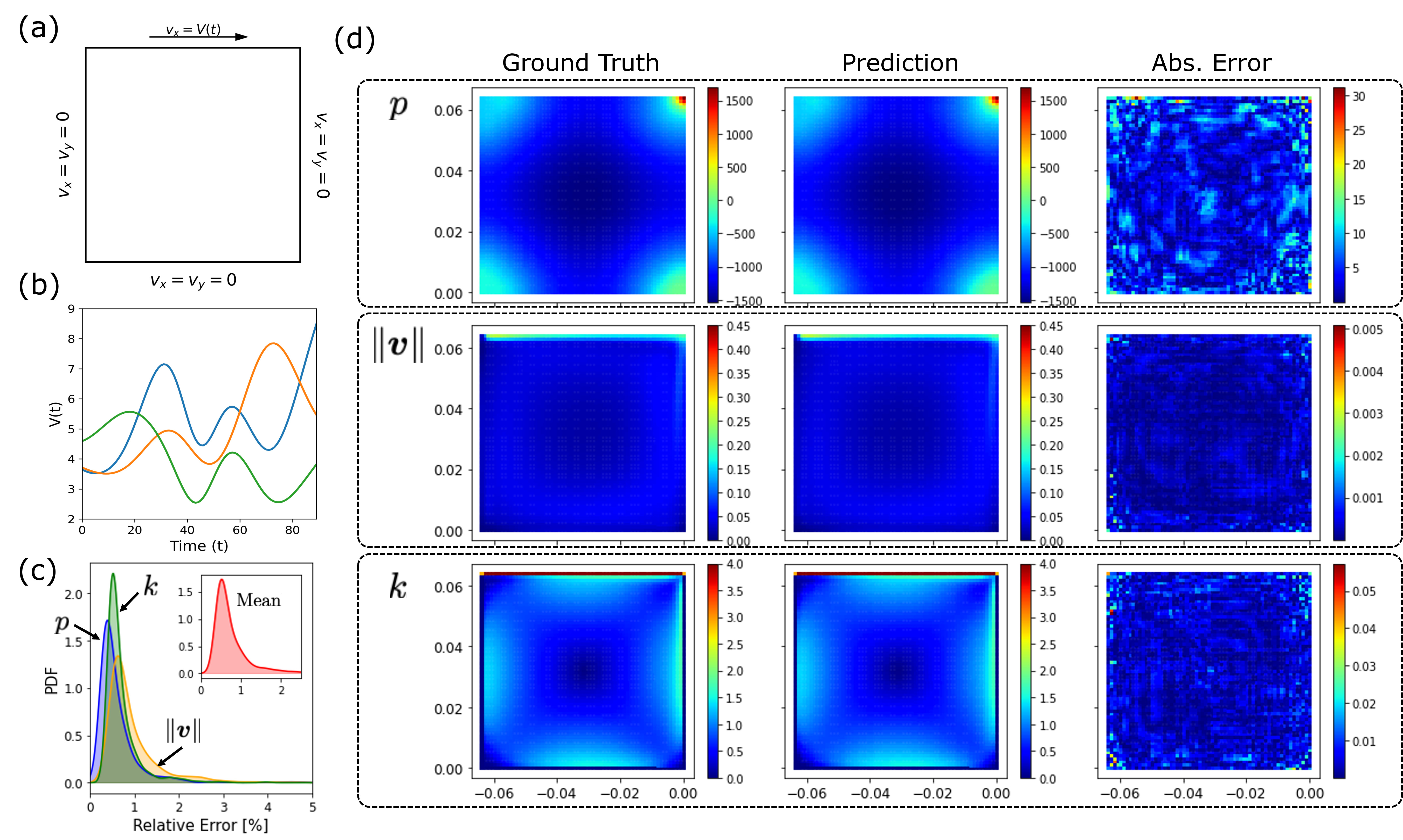
The Lid-Driven Cavity (LDC) problem serves as an initial evaluation of VIRSO’s ability to reconstruct coupled multiphysics fields from a time-varying boundary input. Although defined on a uniform grid, the LDC represents a genuinely hard operator learning problem: the input is a one-dimensional forcing signal $V(t)$ evaluated over 90 discrete time steps, while the target output consists of three coupled fields — pressure $p(x,y)$, velocity magnitude $\|\boldsymbol{v}(x,y)\|$, and turbulent kinetic energy $k(x,y)$ — evaluated over 4,225 interior nodes. This corresponds to a reconstruction ratio of approximately $47{:}1$, with the three-channel output increasing the effective underdetermination further. The governing physics is described by the incompressible Reynolds-Averaged Navier-Stokes (RANS) equations with a $k$-$\varepsilon$ turbulence closure:

$$\nabla\cdot\boldsymbol{v}=0,$$ (4)

$$\frac{\partial\boldsymbol{v}}{\partial t}+(\boldsymbol{v}\cdot\nabla)\boldsymbol{v}=-\nabla p+\nabla\cdot\left[\left(\nu+\nu_{t}\right)\left(\nabla\boldsymbol{v}+\nabla\boldsymbol{v}^{\top}\right)\right],$$ (5)

$$\frac{\partial k}{\partial t}+\boldsymbol{v}\cdot\nabla k=P_{k}-\varepsilon+\nabla\cdot\left[\left(\nu+\frac{\nu_{t}}{\sigma_{k}}\right)\nabla k\right].$$ (6)

The operator learned by VIRSO for this problem is:

$$\mathcal{G}_{ldc}:L^{2}(\mathbb{R}_{\geq 0})\to(L^{2}(\mathcal{Y}_{ldc}))^{3},\quad\mathcal{Y}_{ldc}\subset\mathbb{R}^{2},$$ (7)

approximated as the discrete mapping $\mathcal{G}_{ldc}:\mathbb{R}^{90}\to\mathbb{R}^{4225\times 3}$. The boundary conditions, domain geometry, and operator inputs are illustrated in Figure 2a,b. Details regarding model architecture choices are found in Methods 5.3.

Performance. As shown in Table 1, a 7 integral-kernel layer VIRSO achieves a mean relative $L_{2}$ error of $0.76\%$ across all three output fields, outperforming NOMAD ($0.86\%$), Geo-FNO ($1.11\%$), and GNO ($11.98\%$) at comparable or lower parameter count. The error distributions, shown in Table 7 (Supplementary 6.1) and Figure 2c, are narrow and unimodal across all fields, with interquartile ranges well below $1\%$. Turbulent kinetic energy exhibits the largest variance among the three outputs, consistent with its sensitivity to boundary-layer dynamics near the domain corners where the uniform grid provides insufficient resolution. The 50th percentile reconstruction (Figure 2d) accurately captures the primary recirculating vortex, the shear layer beneath the driven lid, and the secondary corner eddies. Absolute error is highest near the boundary and corner regions, consistent with the known sensitivity of turbulent flow to local geometric curvature.

The uniform $65\times 65$ grid underresolves the turbulent corner eddies that are physically significant and are the primary discriminator between operator architectures. VIRSO’s advantage is expected to increase with proper adaptive mesh refinement near boundary layers, a condition that is satisfied by the subsequent, more realistic benchmarks. With improved architectural choices — a GeLU activation after the spatial block, reordered normalization layers, and a weighted graph Laplacian — the mean error decreases to $0.65\%$, widening the margin beyond all benchmarks ($>0.86\%$) without increasing parameter count or training time.

Figure 2: Lid-Driven Cavity: Problem Formulation and Results. (a) Boundary conditions: no-slip at all walls except the driven lid at $y=1$, where a time-varying forcing signal $V(t)$ prescribes the horizontal velocity. (b) Representative forcing signals $V(t)$ evaluated at 90 discrete time steps, spanning a broad range of transient dynamics. (c) Percentile error distributions from VIRSO for pressure, velocity magnitude, TKE, and overall mean error (blue, orange, green, red). All distributions are centered below $1\%$ with low spread, confirming consistent generalization across the test distribution. (d) 50th-percentile reconstruction: predicted fields, ground truth, and absolute error for pressure, velocity magnitude, and TKE. VIRSO accurately recovers the primary vortex, shear layer, and corner eddies. Elevated absolute error near boundaries and corners reflects the sensitivity of turbulent physics to regions underresolved by the uniform output grid.

Table 1: Model Comparison: Lid-Driven Cavity

Model	Parameters	Mean Relative $L_{2}$ Error (%)
		$p(x,y)$	$\|\textbf{v}(x,y)\|$	$k(x,y)$	Mean
NOMAD	1.63 M	0.65	1.18	0.74	0.86
Geo-FNO	1.68 M	0.94	1.08	1.32	1.11
GNO	0.23 M	2.84	10.89	22.23	11.98
VIRSO	1.62 M	0.62	0.95	0.71	0.76

3.3 PWR Subchannel: Multiphysics Inverse Reconstruction on an Irregular Geometry

The PWR subchannel problem constitutes the first test of VIRSO under the full triple constraint. The output domain $\mathcal{Y}_{sub}$ is an irregular two-dimensional axial cross-section of a reactor subchannel, discretized at 1,733 nodes by the high-fidelity ANSYS Fluent solver. The input consists of two scalar boundary conditions — inlet temperature $T_{in}\in\mathbb{R}$ and axial velocity $v_{in}\in\mathbb{R}$ — together with a one-dimensional axial heat source profile $q(z)=A\sin(\pi z/H)$ evaluated at 100 discrete axial positions along the entire three-dimensional geometry, for a total of 102 input values. The reconstruction ratio for this problem is:

$$\frac{N\times C}{M}=\frac{1{,}733\times 3}{102}\approx 51{:}1,$$ (8)

where $C=3$ output fields — velocity magnitude $\|\boldsymbol{v}(x,y)\|$, temperature $T(x,y)$, and turbulent kinetic energy $k(x,y)$ — are coupled through the governing RANS and energy equations. The input observations are defined on the axial direction ($z$-axis), while the output fields are defined on the transverse cross-section ($x$-$y$ plane) at a single axial point $z=z_{0}$: the input and output domains are geometrically disjoint. This cross-domain structure makes standard operator architectures architecturally misaligned with the problem, as their formulations presuppose coincident input and output domains.

The operator learned is:

$$\mathcal{G}_{sub}:(\mathbb{R})^{2}\times L^{2}(\mathbb{R})\to(L^{2}(\mathcal{Y}_{sub}))^{3},\quad\mathcal{Y}_{sub}\subset\mathbb{R}^{2},$$ (9)

approximated as $\mathcal{G}_{sub}:\mathbb{R}^{102}\to\mathbb{R}^{1733\times 3}$. Details regarding model architecture choices are found in Methods 5.3.

Performance. Table 2 shows that a 4 integral-kernel layer VIRSO achieves a mean error of $0.51\%$ — the best among all models, with a parameter count of only 0.34 M compared to NOMAD’s 0.42 M and Geo-FNO’s 2.70 M. Crucially, the performance advantage is largest for turbulent kinetic energy ($0.88\%$ vs. NOMAD’s $0.96\%$), the output field most sensitive to local geometric complexity near the reactor rod surfaces. This pattern is consistent with VIRSO’s design: the spectral-spatial collaboration mechanism is specifically intended to preserve local high-frequency information near geometrically complex boundaries, which TKE requires more than the smoother pressure and temperature fields.

The percentile statistics in Table 8 (Supplementary 6.1) demonstrate that VIRSO achieves consistently superior performance from the best-case to the 95th-percentile sample, with the narrowest interquartile range of all models. All distributions are centered below $1\%$, and the 50th-percentile reconstruction (Figure 3d) accurately captures wall shear layers near the reactor rod surfaces, the central velocity structure, and the symmetric thermal gradient. Absolute error shows weak spatial correlation with boundary proximity for velocity and TKE, and no systematic pattern for temperature, indicating predominantly stochastic model fluctuations rather than structural reconstruction failures. With further architectural refinements (nonlinear collaboration function, GeLU activation, weighted Laplacian), the mean error decreases to $0.43\%$ at 0.36 M parameters, further extending the advantage over all baselines.

Figure 3: PWR Subchannel: Problem Formulation and Results. (a) Geometry: coolant flow between four reactor rods, analyzed at a fixed axial cross-section. No-slip boundary conditions are enforced on rod surfaces; inlet is at $z=0$. (b) Multimodal boundary inputs: axial heat source profile $q(z)$ at 100 positions and two scalar inlet conditions. These inputs are defined on the axial direction, while outputs are defined on the transverse cross-section — a geometrically disjoint cross-domain configuration. (c) Percentile error distributions (orange: temperature, blue: velocity, green: TKE, red: mean). All distributions centered below $1\%$ with narrow spread. (d) 50th-percentile reconstruction. VIRSO accurately captures wall shear layers, central velocity structure, and symmetric thermal gradient. Weak spatial correlation of error with boundary proximity for velocity and TKE; stochastic fluctuations for temperature.

Table 2: Model Comparison: PWR Subchannel

Model	Parameters	Mean Relative $L_{2}$ Error (%)
		$\|\boldsymbol{v}(x,y)\|$	$T(x,y)$	$k(x,y)$	Mean
NOMAD	0.42 M	0.39	0.27	0.96	0.54
Geo-FNO	2.70 M	1.55	1.06	2.88	1.83
GNO	0.27 M	4.99	0.50	3.47	2.99
VIRSO	0.34 M	0.37	0.28	0.88	0.51

3.4 Wavy-Insert Heat Exchanger: Four-Field Reconstruction on a Highly Irregular Domain

The heat exchanger benchmark represents the most demanding evaluation of VIRSO, combining the highest geometric irregularity, the largest output node count, and a four-component coupled output. The geometry consists of a dimpled cylindrical channel with a wavy tape insert (Figure 4a), whose surface topology breaks any rotational or reflective symmetry present in the subchannel problem. The wavy insert generates large recirculation cells and complex secondary vortex structures that significantly challenge operator learning models lacking local resolution capability AHMED2024104583 .

The output consists of four physical fields at 3,977 nodes on a two-dimensional axial cross-section $\mathcal{Y}_{hx}$: pressure $p(z,y)$ and three velocity components $u_{x}(z,y),u_{y}(z,y),u_{z}(z,y)$. The boundary input is identical in structure to the subchannel problem — two scalar inlet conditions and a 100-point axial heat profile — giving a reconstruction ratio of:

$$\frac{N\times C}{M}=\frac{3{,}977\times 4}{102}\approx 156{:}1.$$ (10)

This is the most severely underdetermined configuration evaluated in this work. The operator is:

$$\mathcal{G}_{hx}:(\mathbb{R})^{2}\times L^{2}(\mathbb{R})\to(L^{2}(\mathcal{Y}_{hx}))^{4},\quad\mathcal{Y}_{hx}\subset\mathbb{R}^{2}.$$ (11)

Details regarding model architecture choices are found in Methods 5.3.

Performance. As shown in Table 3, a 14 integral-kernel (2) layer VIRSO achieves a mean $L_{2}$ error of $0.70\%$, outperforming NOMAD ($0.97\%$) and Geo-FNO ($1.09\%$) at comparable parameter counts, and exceeding GNO ($9.40\%$) by more than an order of magnitude. A 10 integral-kernel layer model ($0.83\%$) similarly outperforms all baselines with fewer parameters than NOMAD or Geo-FNO. The velocity magnitude, computed from predicted components rather than directly trained, shows the lowest reconstruction error among all models, confirming that VIRSO maintains physical consistency across the velocity field tensor without explicit vector-field supervision.

The percentile statistics (Table 9, Supplementary 6.1) show that VIRSO achieves a fully improved sample distribution relative to all baselines, from the best-case to the 95th percentile, with a distribution center of $0.66$–$0.69\%$ and a worst-case error of $0.80\%$ — the narrowest worst-case bound of any model evaluated. The 50th-percentile reconstruction (Figure 4d) accurately captures the two large counter-rotating recirculation cells generated by the wavy insert, the opposing spin directions of the primary vortices, secondary eddies in the component fields, and the pressure response to the insert gap. Elevated absolute error is concentrated near the insert junction and the dimpled channel wall, regions of maximum geometric complexity and steepest physical gradients — precisely the regions where high graph connectivity is needed, as the V-KNN analysis below confirms.

Figure 4: Heat Exchanger: Problem Formulation and Results. (a) Geometry: wavy tape insert inside a dimpled cylindrical channel. Analysis performed on the 2D axial cross-section at $x=0.789$. (b) Boundary inputs: axial heat profile and two scalar inlet conditions, geometrically disjoint from the output cross-section. (c) Percentile error distributions for the 10-layer VIRSO across all output fields. Distributions are centered below $1\%$ with narrow spread. (d) 50th-percentile reconstruction. VIRSO accurately recovers the primary counter-rotating recirculation cells, secondary eddies, and pressure response to the insert gap. Elevated error is concentrated near the insert junction and channel wall, regions of maximum geometric complexity.

Table 3: Model Comparison: Heat Exchanger

Model	Parameters	Mean Relative $L_{2}$ Error (%)
		$p$	$u_{z}$	$u_{y}$	$u_{x}$	$\|u\|$	Mean
NOMAD	2.69 M	0.66	1.01	1.03	0.74	1.43	0.97
Geo-FNO	2.70 M	0.74	1.14	1.14	0.91	1.51	1.09
GNO	0.27 M	3.37	9.89	10.75	11.15	11.82	9.40
VIRSO∗	1.66 M	0.47	0.87	0.86	0.71	1.24	0.83
VIRSO	2.31 M	0.40	0.71	0.66	0.52	1.18	0.70

^∗10-layer VIRSO, 64 modes, function dimension 48.

3.5 Spectral-Spatial Collaboration and Architecture Analysis

The three benchmarks establish VIRSO’s empirical performance. We now probe what VIRSO learns and why the architecture succeeds, using a component-level ablation study on the most demanding benchmark. For reference, the removal of a spatial/spectral block includes removing the entire component and collaboration layer while keeping the other block and the identity skip located after the projection mapping $f$.

Role of cross-domain input embedding. Unlike standard operator benchmarks in which the input and output domains coincide, VIRSO’s nuclear use cases involve a geometrically disjoint input space: the boundary observations are defined on the axial direction while the output fields are defined on the transverse cross-section. This requires that the boundary input be lifted into a latent representation that is then broadcast to all output nodes, rather than evaluated point-wise at their coordinates. To quantify the necessity of this design choice, Table 10 (Supplementary 6.2) isolates the FCN latent embedding and the residual skip connection in the 10-layer heat exchanger model. Removing both components raises the mean error from $0.83\%$ to $4.16\%$, a five-fold degradation. The embedding alone allows for a $4.16\%\to 0.93\%$ reduction, consistent with the interpretation that the FCN extracts the physically relevant low-dimensional structure of the heat profile — primarily its amplitude $A$ and spatial extent $H$ — from the 100-dimensional input representation. Moreover, the addition of a latent embedding can include sequential-based models that can handle varying histories or profile resolutions without retraining. This is demonstrated with the Lid-Driven Cavity implementation of VIRSO (Methods 5.3).

What VIRSO’s spectral-spatial collaboration learns. Table 11 (Supplementary 6.2) decomposes the 10-layer VIRSO model into its spectral-only, spatial-only, and combined forms. Three findings emerge. First, the spectral-only model with residual skip connections ($0.90\%$) substantially outperforms all external benchmarks ($0.97$–$9.40\%$), demonstrating that graph spectral convolution is a primary learning mechanism and that it alone can be sufficient to solve the inverse reconstruction problem at competitive accuracy in the presence of negligible high-frequency physics. Second, removing all residual skip connections from the spectral-only model raises the error from $0.90\%$ to $5.76\%$, revealing that the skip connections serve as local high-frequency feature preservers: the 64 spectral eigenmodes capture the dominant low-frequency physical structure of the heat exchanger flow, but the residual paths preserve the high-frequency modes beyond the truncation threshold that encode wall shear and vortex detail. Moreover, with the combined spatial-spectral analysis, we found in Table 10 (Supplementary 6.2) that the addition of the skip connection after the collaboration layer showed consistent improvement in performance (4.16% to 1.32% from adding skip without embedding and 0.93% to 0.83% from utilizing the skip connection after adding the embedding FCN), reiterating the importance of residual-based learning for gradient flow stability and high-frequency mode preservation within neural operator frameworks. Third, the spatial aggregation component reduces the combined model error from $0.90\%$ to $0.83\%$, a modest but consistent improvement that reflects local fine-tuning of the spectral prediction rather than independent learning — confirmed by the spatial-only model’s catastrophic failure at $16.27\%$. Together, these findings establish that VIRSO’s spectral-spatial collaboration is not architecturally redundant: spectral convolution handles global physical consistency, skip connections preserve high-frequency local structure, and spatial aggregation provides calibration at boundaries and irregular geometric features. For more complex and large-scale geometries, we believe that the spatial analysis would provide a larger contribution towards high-frequency information that cannot be effectively captured by only residual skips and spectral-based learning.

3.6 Graph Construction: The Variable-KNN Principle

Figure 5: Graph Topology and Node Degree Distribution. (a) Mesh geometry of the heat exchanger, adapted to the VIRSO graph node configuration. Higher mesh density is visible near the insert junction and channel walls, corresponding to regions of steepest physical gradients. (b,c) Degree distribution for KNN with $k=30$ and $k=45$: modest variation with slightly elevated connectivity near high-density regions, but insufficient targeting. (d) KNN with $k=93$: high-density regions receive elevated degree, improving performance, but the enforced minimum of 93 throughout the interior introduces significant inefficiency. (e) Radius with $r=0.001$: naturally concentrates high degree near geometrically complex regions; outperforms KNN with $k=30,45$. (f) Radius with $r=0.0015$: matches the maximum degree of KNN with $k=93$ near walls and junctions but maintains a minimum of only 24 in the interior, achieving superior performance with fewer edges. (g) Variable-KNN (V-KNN): explicitly assigns connectivity proportional to local mesh density. Achieves the same maximum degree as (d) and (f) near geometric complexity, maintains minimum degree 45 in the interior, and uses only 270K edges — the most efficient configuration achieving the best overall accuracy.

Graph topology constitutes an underexplored source of inductive bias in graph-based operator learning. The standard KNN graph assigns a uniform minimum degree $k$ to all nodes regardless of their geometric context, which is efficient but physically naive. In finite element analysis, mesh refinement concentrates resolution near geometrically complex regions — walls, corners, and high-curvature surfaces — precisely where physical gradients are steepest. We hypothesize that graph connectivity in neural operators should obey the same principle: nodes in high mesh-density regions, which correspond to regions of high geometric complexity, require higher neighbor counts to propagate physical information across the steep local gradients that arise there. The radius graph provides a natural test of this hypothesis, since it assigns connectivity proportional to local node density. It should be noted that previous concerns about graph regularity and the effect of node hubs towards over-smoothing Vega-Oliveros_2014 ; HUANG2023110556 has not been addressed but most-likely has little effect in the performance of VIRSO due to its combined spatial and spectral architecture and the nature of the regression problems utilized, where variation in flow complexity might require differing node degrees.

Table 12 (Supplementary 6.3) confirms the hypothesis quantitatively with the 10-layer VIRSO model. Among KNN graphs, increasing $k$ uniformly from 30 to 93 reduces the mean error from $0.83\%$ to $0.67\%$, but at a cost of tripling the edge count. Among radius graphs, $r=0.001$ outperforms KNN with $k=45$ ($0.71\%$ vs. $0.79\%$) despite fewer edges, because the radius graph preferentially concentrates high connectivity near the wall and insert junction — the regions shown in Figure 5a to have the highest mesh density. Radius with $r=0.0015$ outperforms KNN with $k=93$ ($0.62\%$ vs. $0.67\%$) while using 284K fewer edges, confirming that targeted high-degree assignment to geometrically complex regions is more effective than uniform high-degree assignment throughout the domain.

These results motivate Variable-KNN (V-KNN), a mesh-density-adaptive graph construction strategy that assigns neighbor counts proportional to local node density, estimated from an initial radius graph at radius $5\times 10^{-4}$. Each node’s degree is set to a fraction of $k_{\max}$ equal to its normalized local density, with a minimum of $k_{\min}$ enforced throughout the interior. With $k_{\max}=134$ and $k_{\min}=45$, V-KNN produces a graph with 270K edges — more efficient than both KNN with $k=93$ (408K) and radius with $r=0.0015$ (292K) — that achieves a mean error of $0.59\%$ (Table 13 Supplementary 6.3), the best result across all graph construction strategies tested. Figure 5g confirms that V-KNN successfully concentrates high connectivity near the dimpled channel wall and wavy-insert junction, while maintaining a controlled minimum degree of 45 in the interior. Beyond reconstruction accuracy, V-KNN provides a hardware efficiency advantage directly relevant to edge deployment. With 270K edges versus 408K for KNN at $k=93$ — the uniform configuration that most closely approaches V-KNN’s accuracy — V-KNN reduces the total edge count by approximately 34% ($\Delta=138\mathrm{K}$ edges). In the spatial aggregation block, inference energy and latency scale approximately linearly with edge count, because each edge corresponds to an independent gather-accumulate operation. V-KNN therefore simultaneously improves spectral eigenmode alignment, reconstruction accuracy, and memory access efficiency — constituting a hardware-aware graph construction principle rather than a purely topological one, applicable to any graph-based operator learning system on irregular physical domains.

To understand the mechanism by which V-KNN improves performance, Table 14 (Supplementary 6.3) repeats the spectral-spatial decomposition on the V-KNN graph. V-KNN improves the spectral-only model with skip connections from $0.90\%$ to $0.71\%$ — a significant gain — while degrading both the spatial-only model and the spectral model without skip connections. This dissociation reveals the mechanism: V-KNN restructures the graph Laplacian’s eigenmodes to better align with the physical structure of the heat exchanger flow, shifting energy toward higher-frequency modes that capture wall shear and vortex detail. This eigenmode restructuring benefits the spectral operator, which explicitly decomposes the signal into graph spectral modes, but penalizes the spatial aggregation operator, which lacks the global spectral view needed to correctly interpret the redistributed connectivity.

3.7 Computational Efficiency and Energy Consumption

Deployment of neural operators for real-time virtual sensing in nuclear systems requires not only predictive accuracy but energy-efficient inference, particularly under edge computing constraints where total I&C power budgets are limited 10545889 ; ALSHARIF20251739 . Most prior neural operator work does analyze inference under hardware deployment constraints. The analysis below is, to our knowledge, the first systematic hardware efficiency characterization of a neural operator that moves towards addressing the compute-versus-memory-bandwidth hierarchy of its target deployment platforms. We report GPU inference statistics for the 310-sample heat exchanger test set on an NVIDIA H200 GPU, using NVIDIA built-in profiling software to measure kernel utilization, memory allocation, instantaneous power, latency, and per-iteration energy consumption (Table 4).

Table 4: Inference Energy and Memory: Heat Exchanger

Model	Param.	FLOPs	GPU%	Mem%	Mem (MiB)	Pwr (W)	Lat. (ms)	Energy (J/it)
NOMAD	2.69 M	11.29 G	30.92	1.12	999.92	196.03	2.35	0.41
Geo-FNO	2.70 M	1.58 G	23.63	2.02	1059.39	139.39	4.94	0.59
GNO	0.27 M	429.49 G	86.78	36.15	1965.99	572.00	20.48	10.07
VIRSO	1.66 M	2.03 G	42.35	5.71	1039.98	193.35	7.77	1.30
VIRSO (Spatial)	0.11 M	0.99 G	32.77	6.95	1031.65	178.15	8.93	1.40
VIRSO (Spectral)	1.58 M	0.98 G	17.34	$<$1	937.93	124.41	8.18	0.86
VIRSO (V-KNN)	1.66 M	2.56 G	64.11	14.93	1153.94	265.02	8.32	1.91

Spatial and Spectral refer to Spatial-Only and Spectral-Only VIRSO.

Memory scalability. All models except GNO allocate approximately 1 GiB of device memory. GNO requires nearly 2 GiB — a consequence of its dense message-passing scheme — and is memory-limited in all three benchmarks. VIRSO uses approximately 0.1 GiB more than NOMAD and Geo-FNO, reflecting the additional graph spectral computation, while remaining well within standard GPU memory constraints.

Latency. From the VIRSO model implementations explored, we found a real-time latency ranging from about 4.29 - 10.32 ms for the Heat Exchanger dataset of 3,977 evaluation nodes. The sequential aspect of VIRSO is responsible for the latency in model inference. This is demonstrated by Table 16 with the 14-layer VIRSO model requiring approximately three times the latency for predictions than a 2-layer lightweight model with width 48 and mode count of 40. Compared to other neural operators, VIRSO only requires slightly more time for predictions with latency statistics within the same order of magnitude as NOMAD and Geo-FNO. Such computational requirements are a drastic improvement to previous graph methods that are either unable to scale to our chosen benchmarks or have high computation requirements such as GNO (Table 4, 16).

Comparison with ANSYS Fluent. For the Heat Exchanger and Subchannel, our 2D slice results originate from full 3D simulation. To provide an estimate of the amortized inference speed up of VIRSO compared to Fluent, we must observe the Lid-Driven Cavity which was purely two dimensional with 4,225 evaluation nodes. ANSYS Fluent required approximately 36 minutes to generate a solution on an AMD EPYC 7763 (“Milan”) CPU while our VIRSO model configured for the LDC use case required around 88 milliseconds on an NVIDIA H200 GPU which corresponds to a speedup of more than 4 orders of magnitude. VIRSO is able to improve upon the high computational requirement of preceding graph methodologies and provide highly-accurate irregular field reconstruction in real-time.

Power Draw. In Table 4, we also found that VIRSO without V-KNN required similar power draw to NOMAD and slightly higher draw (within 60W) than Geo-FNO. The spectral only model required lower instantaneous power than the other operator models, emphasizing the improved computational efficiency of VIRSO compared to previous graph operators such as GNO which required approximately half a kilowatt of power.

Energy cost of spatial aggregation. The primary energy cost of VIRSO relative to NOMAD and Geo-FNO is the local spatial graph convolution. Table 4 also isolates this cost: the spatial-only component requires 1.40 J/it versus 0.86 J/it for the spectral-only component with skip connections. This is a direct consequence of the message-passing implementation in PyG PyG , where energy consumption scales with total edge aggregation operations — approximately linear in the product of node count and average degree. The combined VIRSO model (1.30 J/it) falls between its components because the collaboration mechanism partially offloads learning to the spectral path, reducing the effective contribution of the spatial path.

Performance trade-off. VIRSO consumes 3–5 times more energy per inference than NOMAD or Geo-FNO at their full parameter counts (Table 4), while achieving approximately 20–30% lower mean error. For applications where energy budget is the primary constraint, the spectral-only VIRSO configuration (0.86 J/it) provides the best trade-off: it consumes only twice the energy of NOMAD while outperforming all external baselines on the heat exchanger benchmark. Accuracy-critical scenarios with high-frequency physics would then required the inclusion of the spatial block.

Energy-delay product. To jointly characterize the latency and energy trade-off, we compute the energy-delay product $\mathrm{EDP}=E_{\mathrm{iter}}\times t_{\mathrm{lat}}$, which penalizes configurations that sacrifice latency for energy savings or vice versa. From Table 4, GNO incurs an EDP of $10.07\times 20.48\approx 206$ J$\cdot$ms — more than $20\times$ higher than the full VIRSO configuration ($1.30\times 7.77\approx 10.1$ J$\cdot$ms). The spectral-only VIRSO achieves the most favorable EDP among graph-based operators ($0.86\times 8.18\approx 7.0$ J$\cdot$ms), and approaches Geo-FNO ($0.59\times 4.94\approx 2.9$ J$\cdot$ms) and NOMAD ($0.41\times 2.35\approx 0.96$ J$\cdot$ms) while delivering substantially lower reconstruction error on the heat exchanger benchmark.

Power-normalized accuracy. We define a power-normalized accuracy metric $\eta=(100\,/\,\bar{e}_{L_{2}}[\%])\,/\,P[\mathrm{W}]$, quantifying reconstruction accuracy delivered per watt of instantaneous GPU power. The spectral-only VIRSO achieves $\eta=(100\,/\,0.90)\,/\,124.41\approx 0.89\;\%^{-1}\mathrm{W}^{-1}$ and full VIRSO configuration achieves $\eta=(100\,/\,0.83)\,/\,193.35\approx 0.62\;\%^{-1}\mathrm{W}^{-1}$, compared to $\eta=(100\,/\,0.97)\,/\,196.03\approx 0.53\;\%^{-1}\mathrm{W}^{-1}$ for NOMAD. Despite requiring more energy per inference in absolute terms, the spectral-only and full VIRSO delivers superior reconstruction accuracy per unit of power consumption. These values reflect device-level GPU measurements on the H200 and are not directly comparable to the board-level Jetson measurements in Table 6.

A 2-layer lightweight VIRSO (0.26 M parameters, 0.54 J/it, width 48, and mode count of 40) achieves comparable energy consumption to the original Geo-FNO and NOMAD and their lightweight versions while maintaining solid performance compared to high performance degradation of the lightweight versions of Geo-FNO and NOMAD (Table 15 and Table 16).

In terms of latency, lower number of layers reduces prediction time, with the 2-layer model (4.29 ms) providing improved latency comparable to other operators without extreme performance degradation such as NOMAD’s transition to lightweight (Table 15 and Table 16).

The energy analysis establishes that the appropriate VIRSO configuration is task-dependent: the full spectral-spatial model is preferred when accuracy is the governing constraint, the spectral-only model when energy efficiency is primary, and the lightweight model when both constraints are simultaneously binding.

For accuracy-critical applications where computational resources are unconstrained, the full spectral-spatial VIRSO with V-KNN (1.91 J/it) is preferred. For edge-deployed sensing where total I&C power budgets impose strict limits, the spectral-only configuration (0.86 J/it) provides the best accuracy-energy trade-off while outperforming all baselines but risking the loss of higher frequency analysis and calibration with the spatial block. For the most resource-constrained settings, the 2-layer lightweight model (0.54 J/it) maintains reconstruction errors below 2%, substantially better than comparably sized alternatives, at energy consumption comparable to conventional operator methods. Lastly, latency-constrained applications within an Nvidia H200 device would require the lowest layer count for VIRSO, such as the 2-layer version (4.29 ms). In addition, graph construction and degree count are other considerations with higher neighbors, or essentially increased aggregation, typically resulting in higher power draw for the combined spatial-spectral analysis (shown with V-KNN in Table 4).

Table 5 consolidates accuracy and hardware efficiency across all evaluated configurations on the heat exchanger benchmark, enabling direct comparison across the accuracy–energy trade-off space. The spectral-only VIRSO occupies the Pareto frontier among graph-based operators: it achieves lower reconstruction error than all baselines while requiring 0.86 J/it and 8.18 ms latency. The 2-layer VIRSO provides NOMAD-comparable energy consumption (0.54 J/it) and latency (4.29 ms) at substantially lower reconstruction error than any lightweight baseline (1.95% vs. 4.21–8.24%), establishing VIRSO as the preferred architecture across the full range of accuracy-constrained deployment conditions.

Table 5: Accuracy–Efficiency Summary: Heat Exchanger (H200, device-level GPU measurements)

Model	Mean $L_{2}$ (%)	FLOPs	Energy (J/it)	Lat. (ms)	EDP (J$\cdot$ms)
GNO	9.40	429.49 G	10.07	20.48	206.2
Geo-FNO (full, 2.70 M)	1.09	1.58 G	0.59	4.94	2.91
Geo-FNO (light, 0.26 M)	4.21	1.16 G	0.56	5.10	2.86
NOMAD (full, 2.69 M)	0.97	11.29 G	0.41	2.35	0.96
NOMAD (light, 0.26 M)	8.24	1.28 G	0.23	2.00	0.46
VIRSO (2-layer, 0.26 M)	1.95	0.61 G	0.54	4.29	2.32
VIRSO (spectral-only, 1.58 M)	0.90	0.98 G	0.86	8.18	7.03
VIRSO (10-layer full, 1.66 M)	0.83	2.03 G	1.30	7.77	10.1

EDP = Energy $\times$ Latency. Lightweight variants use ${\approx}0.26$ M parameters (Tables 15 and 16). VIRSO (10-layer full) accuracy is the 1.66 M configuration (VIRSO^∗, Table 3); hardware numbers are from Table 4. All values are H200 device-level GPU measurements and are not directly comparable to Jetson board-level measurements in Table 6.

3.8 Towards Edge Deployment: Embedded Inference on Resource-Constrained Hardware

Unlike conventional surrogate models evaluated post hoc, VIRSO is designed such that its operator decomposition aligns with hardware execution constraints, enabling it to function as a physically realizable sensing instrument under edge conditions.

Table 6: Embedded inference performance of pretrained 10-layer (full and spectral-only) and the 2-layer VIRSO model.

Model	Param.	FLOPs	Avg. Lat. (ms/it)	Avg. Pwr (W)	Energy (J/it)	Peak RAM (GB)	Mean L2 (%)
10-L (Full)	1.66 M	2.04 G	562.92	7.58	4.72	5.16	0.84
10-L (Spec.)	1.58 M	0.98 G	58.77	7.06	0.84	5.14	0.91
2-L	0.26 M	0.61 G	104.03	7.51	1.25	5.32	1.96

N-L represents N spectral-spatial layers for VIRSO, FLOPs per inference sample are computed via torch.profiler on the 3,977-node Heat Exchanger test set.

The preceding analysis characterizes the energy–accuracy trade-off of VIRSO on datacenter-scale GPUs. A related practical question is whether the same pretrained operator is hardware-portable and can also be executed on embedded hardware, where memory, board-level power, and thermal margins are substantially more limited. This question is relevant to virtual sensing deployments in which inference may need to be performed near the sensing hardware rather than on remote accelerator infrastructure.

Experimental setup. We evaluated the three pretrained VIRSO models, 10-Layer Full, 10-Layer Spectral-Only, 2-Layer Full, on an NVIDIA Jetson Orin Nano (8 GB), an embedded platform with an Ampere-based GPU and shared system memory. Our analysis is deployed towards the Heat Exchanger dataset with the same 3,977-node output. The 10-Layer models utilize a width and mode count of 48 and 64 while the 2-Layer model has the same width but only 40 spectral modes. All three models are trained on a $k=30$ KNN graph. No retraining, quantization, pruning, or architecture-specific modification was introduced. Inference was performed on the full 310-sample Heat Exchanger test set, and reported values correspond to the mean over three independent runs with board-level telemetry recorded throughout execution. A summary of the results is shown in Table 6 where we display average latency, power, energy per iteration, peak RAM usage, and the mean relative L2 error over all multiple outputs in the Heat Exchanger dataset.

Latency. Across the three runs, the 10-layer VIRSO achieved an average latency of $562.92$ ms/iteration (1.78 samples/s) for the full version and $58.77$ ms/iteration (17.0 samples/s) for the spectral-only version (Table 6). The 2-layer model achieved an average latency of $104.03$ ms/iteration (9.61 samples/s). Although the resource-constrained operation of the Jetson Nano results in a significantly higher latency than the NVIDIA H200, VIRSO’s efficient graph analysis allows for a sub-second per-sample regime on embedded hardware without deployment-specific simplification. Future acceleration is required to push latency, especially for the full 10-layer model, to realistic real-time conditions (<100ms). An unexpected trend in the latency results is that the 10 layer spectral-only latency is lower than the 2-layer model. Compared to an NVIDIA H200, the Jetson Nano struggles significantly more on the point-wise aggregation within the spatial block, making such local analysis the main bottleneck for latency instead of layer count which was observed with the H200 analysis. It is most likely that the sophisticated optimization of the H200, compared to the resource-constrained Nano, is able to better handle the local aggregation algorithms implemented by the python-based PyG library PyG . Quantitatively, the full 10-layer model is $562.92\,/\,58.77\approx 9.6\times$ slower than the spectral-only configuration on the Jetson Nano, whereas the corresponding latency difference on the H200 is less than 0.5 ms (Table 4). This hardware-dependent dissociation reflects a fundamental difference in memory-subsystem architecture: graph message passing is a memory-bandwidth-bound operation whose irregular scatter-gather pattern incurs disproportionate cost on the Jetson Orin Nano’s unified LPDDR5 memory, whereas spectral convolution reduces to dense matrix multiplications that are compute-bound and therefore hardware-portable across the two platforms. The spectral-only configuration eliminates this bandwidth bottleneck entirely, delivering 17.0 samples/s on the Jetson Nano without retraining or architectural modification.

Power and energy. The average board-level power during inference for all models ranged from $7.06$ W (spectral-only configuration) to $7.58$ W (full 10-layer), measured as the mean VDD_IN rail power integrated over the full 310-sample evaluation window using tegrastats at 20 ms sampling intervals. This board-level measurement encompasses GPU, CPU, and shared-memory activity throughout inference. All configurations sustain $<$10 W total board power with only slight dependence on model architecture or layer count, confirming operational compatibility with strict embedded power envelopes. With the Jetson Nano, we are able to address the high power consumption seen with the H200 in Table 4 on the NVIDIA H200. In other words, the main bottleneck for the real-time performance on the Jetson Nano, within the context of the benchmarks presented, is model latency which is emphasized in the energy consumption results. The full 10-layer VIRSO model achieved $4.721$ J/iteration due to its higher latency while the spectral only was less than one joule. These values are not directly comparable to the datacenter GPU measurements in Table 4, because the telemetry domains differ (board-level on Jetson versus device-level on H200). Nevertheless, the observed board power remained within a single-digit watt range throughout execution.

Resource stability. Resource usage was stable across runs. Peak RAM usage and observed temperature for all models was no higher than 5.32 GB and 47.93^∘C (maximum for both is the full 10-layer). The lowest Peak RAM was 5.14 GB and the lowest temperature was 44.56^∘C (both for the full 2-layer). GPU utilization over all three models averaged from 17.65% (2L) to 32.95% (10L full) and peaked from 67% (2L) to 79% (both 10L models). Together, these measurements indicate that the full inference pipeline completed on the embedded platform without memory exhaustion or thermal instability.

Performance trade-off. As expected, the reconstruction performance of all three models in Table 6 is almost identical to the performance on the NVIDIA H200. As a result, the energy-performance trade-off is similar. For accuracy-critical applications, the full 10-Layer model is preferred while the spectral-only version is preferred for energy-constrained and latency-constrained conditions. For ideal real-time performance on the Jetson Nano, latency is the main concern, and the spectral-only version of VIRSO provides a desired <100ms latency. It should be noted that excluding the use of the spatial block should be avoided, especially with large-scale, complex applications where the local aggregation can have a larger contribution to reconstruction error. Further work within edge computing devices such as the Jetson Nano should address accelerating VIRSO to the desired latency standards. We further quantify computational complexity in terms of floating-point operations (FLOPs), demonstrating that VIRSO achieves lower algorithmic cost while reducing memory-bound operations through localized spatial computation.

Critically, the ablation analysis (Section 3.5) and energy analysis above reveal a hardware-architecture correspondence that is, to our knowledge, uncharacteristic in prior operator learning work: the spectral path’s dominant operations are dense matrix multiplications (compute-bound), while the spatial path’s dominant operations are irregular edge gather-scatter (memory-bandwidth-bound). This dissociation directly motivates the deployment-aware architectural choice of removing the spatial block and presents VIRSO as a flexible architecture, unique among other operators. In other words, when encountering strict computational constraints and negligible high-frequency physics, the spectral-only configuration can be utilized, positioning VIRSO as a hardware-aligned design that can be uniquely configured to specific edge-compute applications. When complex and higher frequency physics is no longer negligible, the spatial portion is then required and provides a calibration for improved accuracy and sophisticated irregularity-handling with increased computation that still is far below previous graph methodologies and comparable to existing solutions. Further work is necessary for hardware-based acceleration of the entire VIRSO model, but we present VIRSO’s initial feasibility for edge deployment.

4 Discussion

These results suggest a shift from simulation or sensor-centric paradigms toward computation-driven sensing, where learned operators act as primary measurement mechanisms rather than post-processing tools. The central contribution of this work is repositioning neural operators from surrogate acceleration models to sensing primitives: inference here is not merely prediction but a form of measurement, conditioned on sparse boundary observations and constrained by the hardware on which it executes. A surrogate model is evaluated offline against a known solution; a sensing primitive operates continuously, in real time, under power and latency constraints that are as binding as the accuracy requirement. VIRSO is designed to satisfy all three constraints simultaneously, establishing a natural graph-based operator analysis towards highly irregular geometries as a deployable sensing modality rather than a computational convenience. This is a sensing problem in a precise and non-trivial sense: the quantities to be measured reside in the interior of a domain that is structurally inaccessible to direct instrumentation, sensors are confined to accessible boundary surfaces, and the inference must operate in real time from the sensor data alone. VIRSO provides an architecture that treats this configuration as a primary design target rather than a limiting special case: sparse cross-domain observations, irregular output geometry, and coupled multiphysics outputs are addressed simultaneously by coordinated design choices rather than post-hoc workarounds. Uniquely among neural operators, VIRSO provides an improved graph spectral-spatial decomposition with the explicit goal for eventual edge deployability — a principle standard in hardware-efficient deep learning for CNNs and transformers but, to our knowledge, absent from the operator learning literature prior to this work. The result is an architecture with configuration choices that are determined by hardware characteristics rather than by post-hoc compression. The spectral path and spatial analysis can both preserve the sophistication of graph-based analysis and provide more efficient reconstruction than previous graph methods that is hardware-portable across the full range of deployment hardware, from H200 datacenter GPUs to embedded accelerators such as the Jetson Orin Nano, without retraining, quantization, or architecture-specific modification. Moreover, the spectral block is compute-bound while the spatial path is memory-bandwidth-bound. In the case of negligible high-frequency physics and strict computational requirements, the latter path can be selectively omitted at the edge — producing a virtual sensor that still successfully recovers complete interior field states from boundary readings at reconstruction ratios between 47:1 and 156:1, within error bounds consistent with operational monitoring requirements, at inference latencies compatible with real-time control.

A primary contribution of VIRSO’s sensing accuracy is the spectral graph convolution, which operates on the $m$ largest eigenmodes of the normalized graph Laplacian. The physical interpretation is direct: low-index Laplacian eigenmodes correspond to domain-spanning spatial patterns analogous to the long-wavelength modes of a continuous field. Convolving the boundary-encoded node features against these eigenmodes propagates the boundary signal globally across the interior in a single operation, enabling the operator to reconstruct interior field structure consistent with boundary physics without relying on iterative local message-passing. This global propagation is the computational mechanism underlying the sensing operator’s ability to recover interior fields at high reconstruction ratios. Critically, the residual skip connections following each spectral convolution are not incidental training components but functional elements of the sensing architecture. Ablation experiments confirm this quantitatively: removing residual connections from the spectral model raises mean relative $L_{2}$ error from $0.90\%$ to $5.76\%$, a $6.4\times$ degradation concentrated in the high-gradient boundary-layer and recirculation regions where wall shear and vortex signatures reside. The $m=64$ spectral eigenmodes capture the dominant low-frequency field structure; the residual paths preserve high-frequency physical information at spatial frequencies beyond the truncation threshold. Together they constitute a two-pathway sensing architecture: global eigenmode projection for long-range field recovery, residual preservation for local physical fidelity. From a hardware perspective, the spectral convolution is structurally compute-bound: the dominant operations are dense matrix multiplications of the form $\mathbf{Q}_{m}\cdot\mathbf{K}\times_{1}\mathbf{Q}_{m}^{\top}\cdot\mathbf{v}_{t}$, whose arithmetic intensity is insensitive to the memory-bandwidth hierarchy of the target device. This compute-bound profile results in its low latency performance on the Jetson Nano and motivates the flexibility aspect of VIRSO where strict resource constraints can potentially utilize a spectral-only configuration.

The spatial graph convolution improves sensing accuracy in a calibration-based role whose contribution level geometry and physics dependent. Models retaining only spectral convolution and residual connections achieve mean relative $L_{2}$ errors within $0.1$–$0.2$ percentage points of the full VIRSO architecture while requiring substantially fewer parameters and lower inference energy. Spatial aggregation provides calibration, especially for use cases that consist of high-frequency modes such as the Heat Exchanger, where maximum geometric complexity and four coupled output channels jointly exceed what $m=64$ spectral modes can represent without local refinement. This geometry-dependence is physically interpretable: the relative contribution of the spatial branch is governed by the ratio of geometric complexity to the number of retained spectral modes, and the two components are complementary rather than redundant. Critically, the spatial aggregation branch is memory-bandwidth-bound: edge gather-scatter operations over irregular adjacency lists incur cost proportional to the memory bandwidth of the target device rather than its arithmetic throughput. This architectural distinction is directly observable in the deployment measurements: on the H200, adding the spatial branch changes inference latency by less than 0.5 ms relative to the spectral-only configuration, whereas on the Jetson Orin Nano’s unified LPDDR5 memory subsystem, the same branch inflates latency by $9.6\times$ ($562.92$ ms versus $58.77$ ms, Table 6). This hardware-dependent dissociation provides the principled basis for selecting the spectral-only configuration as the preferred edge-deployment variant: it eliminates the memory-bandwidth bottleneck while retaining the dominant learning pathway, delivering 17.0 samples/s on the Jetson Nano without any model modification. While this was successful for the 2D Heat Exchanger, we emphasize caution and further evaluation towards the removal of the spatial block. Large-scale applications with strong presence of high frequency physics might require the local calibration that the spatial aggregation analysis provides.

The graph construction strategy encodes a physical principle that has direct implications for sensor system design. Physical sensing systems resolve geometric complexity adaptively: measurement density concentrates near boundaries, interfaces, and regions of steep physical gradients, where the sensing task is most constrained and the physical signal content is highest. The V-KNN strategy embeds this same principle into the computational graph: edge connectivity is assigned in proportion to local mesh density, which in numerical simulation meshes corresponds directly to regions of steep physical gradients. This density-proportional connectivity reorients the eigenmodes of the graph Laplacian to align with the underlying flow structure, providing the spectral sensing operator with physically meaningful basis functions rather than artifacts of a geometrically uninformed graph. Empirically, V-KNN achieves $0.58$–$0.59\%$ mean error on the heat exchanger benchmark with 270,000 edges, both the highest sensing accuracy and the most efficient edge configuration evaluated. The V-KNN principle, that graph topology should encode physical geometric structure as an inductive bias, in direct analogy with adaptive mesh refinement in numerical simulation, is applicable to any graph-based sensing or operator learning system operating on irregular physical domains. V-KNN additionally carries a hardware efficiency consequence that is independent of its spectral eigenmode argument: with 270K edges versus 408K for the uniform KNN graph at $k=93$, the configuration that most closely matches V-KNN’s reconstruction accuracy, V-KNN reduces the total edge count by 34%. Since spatial aggregation energy and latency scale approximately linearly with edge count, this targeted connectivity reduction translates directly into lower memory bandwidth demand and fewer gather-accumulate operations per inference cycle, without degrading the spectral convolution path on which accuracy primarily depends. V-KNN therefore simultaneously encodes physical geometry as inductive bias, reduces deployment-time memory pressure, and achieves the highest reconstruction accuracy of any graph construction strategy evaluated.

A central operational advantage of VIRSO is the inference speed. Once trained, the model reconstructs complete multiphysics state fields for the Lid Driven Cavity in approximately 88 ms per sample, a speedup of more than 4 orders of magnitude over the ANSYS Fluent reference solver. This latency reduction is structurally inaccessible to physics-based reconstruction methods (FEM), which must resolve the coupled PDE system for each new sensor reading. In a deployed virtual sensing system, VIRSO can continuously assimilate new boundary observations and update interior field estimates on a timescale commensurate with the physical dynamics being monitored, rather than the timescale of the underlying simulation. This continuous real-time updating is the operational definition of a virtual sensor: an instrument that infers the unmeasured state of a system from measured signals in real time.

VIRSO provides drastically reduced latency and energy consumption compared to previous graph-based methodologies. The vanilla GNO architecture incurs an energy-delay product of $10.07\times 20.48\approx 206$ J$\cdot$ms on the H200, more than $20\times$ higher than the full VIRSO configuration ($1.30\times 7.77\approx 10.1$ J$\cdot$ms) and more than $29\times$ higher than the spectral-only variant ($0.86\times 8.18\approx 7.0$ J$\cdot$ms). The spectral-only VIRSO approaches the energy-delay product of Geo-FNO ($0.59\times 4.94\approx 2.9$ J$\cdot$ms) and NOMAD ($0.41\times 2.35\approx 0.96$ J$\cdot$ms) while delivering substantially lower reconstruction error on the most demanding benchmark. Embedded deployment on the Jetson Orin Nano confirms that the spectral-only configuration sustains $7.06$ W board-level power (VDD_IN rail, tegrastats) and 17.0 samples/s inference throughput without retraining or architectural modification, satisfying the sub-10 W continuous power envelope required for edge-deployed instrumentation and control systems. The full 10-layer model sustains the same sub-10 W power budget (7.58 W) but at 1.78 samples/s, with latency as the binding constraint rather than power. These results, with sub-10 watt power and sub-second latency, position VIRSO as a hardware-portable architecture for edge deployment but also motivate inference acceleration as the primary engineering priority.

VIRSO’s parameter efficiency under compression is a second operational consideration. At parameter counts below 300K, VIRSO degrades by $2$–$3\times$ in mean relative error, while competing architectures degrade by $4$–$8\times$ under identical constraints. This superior compression efficiency reflects the spectral-spatial architecture’s ability to encode physically meaningful global and local structure compactly in the spectral eigen-basis and local spatial calibration. From a hardware deployment perspective, this compression resilience is consequential: the 2-layer VIRSO configuration achieves 1.95% mean error at 0.54 J/it and 4.29 ms latency on the H200, energy and latency comparable to full-scale Geo-FNO and NOMAD, while matching their parameter count at 0.26 M. No competing lightweight architecture approaches this error level at comparable resource cost (Table 5). This positions VIRSO as the preferred foundation for future hardware-specific optimization, including operator fusion, INT8 quantization of the spectral dense-matmul path, and structured pruning of spatial edges, all of which are tractable without the catastrophic accuracy degradation observed in compressed alternatives.

The current implementation has three limitations that define the highest-priority directions for future work. First, all experiments evaluated steady-state fields; transient virtual sensing, including load-following reactor modes and thermal transient scenarios, requires time-dependent field reconstruction. Extending VIRSO to spatiotemporal sensing by incorporating recurrent or attention-based temporal encoding is a natural architectural extension. Second, the energy consumption of the full spectral-spatial configuration at deployment scale remains elevated relative to lightweight alternatives; structured pruning of the spatial branch can be utilized but should be avoided for large-scale applications. Hardware-specific operator fusion are tractable paths toward edge-deployable configurations as well as algorithmic optimizations, especially since VIRSO is shown to result in less performance degradation compared to other operators and can potentially avoid severe increases in error after efficiency-related integrations. Third, with our evaluation of VIRSO on the Jetson Nano, we found that latency is the main bottleneck and further work towards inference acceleration will be vital for realistic resource-constrained deployment. Two hardware acceleration pathways are tractable without architectural modification. The spectral convolution path reduces to a sequence of dense matrix multiplications that are amenable to TensorRT kernel fusion; based on reported gains for transformer-class workloads on Ampere-architecture GPUs, this pathway is projected to reduce spectral-only Jetson latency by $2$–$4\times$, targeting the sub-15 ms regime. The spectral path’s arithmetic profile (dense, low-precision-tolerant matrix multiplications) is additionally compatible with FP16 and INT8 quantization without structural change, whereas the spatial aggregation path’s irregular memory access patterns are not, providing a further architectural basis for the spectral-only deployment mode as the preferred quantization target. Therefore, a distinct optimization pathway is required for the spatial aggregation component. Improving the spatial pathway remains important due to its potential to enable broader calibration and improved fidelity in more complex, large-scale application settings. Fourth, and most critically, cross-geometry generalization, training VIRSO on one physical geometry and performing virtual sensing on a structurally distinct one without retraining, has not yet been evaluated. This is the central open question for the approach. A virtual sensor that generalizes across geometries would be qualitatively more useful than one requiring independent training per component: it would establish that VIRSO captures transferable physical structure rather than geometry-specific spectral patterns, enabling multi-unit deployment without proportional data generation and training cost. We regard cross-geometry generalization as the primary experimental extension of this work.

Within this context, the reliability of such inference remains fundamentally tied to rigorous uncertainty quantification (UQ) and systematic data analysis, as both two-phase flow simulations and learning-based models introduce nontrivial sources of uncertainty that directly impact predictive confidence and operational robustness foutch2025ai ; kobayashi2024ai ; kumar2019influence ; kumar2022multi . From a system-level perspective, the integration of machine learning with two-phase flow simulations, real-time signal processing, and advanced sensing modalities extends beyond performance prediction toward physically realizable digital twin architectures. In this paradigm, models trained on coupled simulation and sensor data function not only as predictive tools but also as virtual sensing mechanisms capable of estimating inaccessible internal states, enabling continuous monitoring, adaptive optimization, and closed-loop system awareness in operational environments kabir2010hardware ; kabir2010theory ; kabir2010watermarking . Consequently, this integration supports a transition from passive diagnostics to active, data-driven operation, with direct implications for improving heat pipe performance, enhancing reactor reliability, and enabling higher levels of autonomy in advanced reactor systems (alam2019small1, ; alam2019small2, ; kabir2010non, ; kabir2010loss, ).

In conclusion, we have demonstrated that sparse boundary-to-interior multiphysics field reconstruction, the core virtual sensing problem for under-instrumented physical systems, is achievable at operational accuracy and latency on irregular geometries, a task that neither physics-based solvers nor prior graph-based neural operator architectures address as a primary design target. VIRSO establishes two contributions that are, to our knowledge, without precedent in the neural operator literature. First, it demonstrates that spectral-spatial graph operator learning, with mesh-informed graph construction and residual preservation of high-frequency field features, provides the irregular geometry handling, boundary-sensing tolerance, and multiphysics coupling resolution required by this class of inverse sensing problems. Second, and more broadly, it establishes that neural operator architecture can be designed with target hardware in mind, producing a model towards deployability and portability whose spatial-spectral analysis provides efficient computation and allows for flexibility when the operating point shifts from full spectral-spatial on unconstrained compute to spectral-only on strictly resource-constrained edge devices, without retraining, quantization, or accuracy sacrifice on the dominant learning pathway. The sensing principle demonstrated here, inferring complete interior field states from sparse boundary observations by learning the governing Green’s function implicitly from data, is architecture-agnostic and domain-agnostic. It applies wherever the triple constraint of geometric irregularity, sparse cross-domain sensing, and coupled multiphysics output co-occurs: cardiovascular monitoring, subsurface resource assessment, structural health sensing, and industrial process control. VIRSO provides both a practical virtual sensor and a foundational operator-learning framework for the broader class of physical systems in which the most important quantities are precisely the ones that cannot be directly measured. The enabling insight is that the operator and the hardware are not independent concerns: VIRSO’s combined spectral-spatial analysis pushes graph-based operators towards edge deployment and is flexible in its configuration since the spatial refinement can be omitted if high-frequency calibration is not needed and strict resource constraints exist, effectively positioning the architecture itself as a deployment strategy. This is what it means to treat a neural operator as a sensing instrument rather than a model.

By transforming operator inference into a deployable sensing mechanism, this work reframes computation as a form of measurement, bridging the gap between numerical modeling and physical instrumentation.

5 Methods

5.1 Generation of Reference Multiphysics Fields Using ANSYS Fluent

Reference interior field solutions were generated using ANSYS Fluent AnsysFluent2024 , executed on AMD EPYC 7763 (“Milan”) CPU nodes to produce high-fidelity steady-state solutions for three nuclear thermal-hydraulic geometries. The Lid-Driven Cavity (LDC) is inherently two dimensional while the PWR Subchannel and compact Heat Exchanger were each modeled as full three-dimensional geometries; for VIRSO evaluation, a single two-dimensional axial slice was extracted from the Subchannel and Heat Exchanger to yield the irregular unstructured meshes on which operator learning is performed. Boundary conditions defining the sparse input signals (inlet velocity profiles, wall temperatures, and pressure boundary values) were varied systematically across the dataset to produce diverse operating states that span the relevant physical envelope of each geometry.

Critically, ANSYS Fluent solves the governing Navier-Stokes and energy equations as a forward problem: given a complete specification of boundary conditions on $\partial\Omega$ and geometry $\Omega$, the solver produces the interior multiphysics field $\mathbf{s}(\mathbf{x})$ at all mesh nodes $\mathbf{x}\in\Omega$ through iterative PDE discretization. This forward computation requires resolving the full coupled equation system and incurs computational latency that precludes real-time operational use. VIRSO addresses the inverse problem: given only sparse observations $\{u_{i}\}_{i=1}^{M}$ of the boundary condition values, sampled at $M\ll|\Omega|$ locations on the inlet domain $\mathcal{X}$, infer the complete interior field $\mathbf{s}(\mathbf{x})$ at all $N$ mesh nodes of the output domain $\mathcal{Y}$ without access to the full boundary specification or any intermediate PDE solve. Across the three benchmarks, the reconstruction ratio $N/M$ ranges from approximately 47:1 (LDC) to 51:1 (Subchannel) to 156:1 (Heat Exchanger), defining genuinely underdetermined inverse problems in which many smooth interior fields are consistent with the same sparse boundary observations. This forward/inverse separation ensures that VIRSO receives no privileged physical information beyond what a boundary sensor array would provide in a deployed instrumentation system, and it defines the information asymmetry (Forward: Complete BCs $\rightarrow$ Interior Field; Inverse: Sparse BCs $\rightarrow$ Interior Field) that motivates the architectural choices described below.

Training, validation, and test splits were constructed by partitioning across distinct boundary condition instances to ensure that no operating state seen during training appears in evaluation.

5.2 VIRSO Architecture and V-KNN Graph Construction

Problem Formulation as Operator Learning

VIRSO learns the nonlinear operator $\mathcal{G}:\mathbf{u}_{\mathcal{X}}\mapsto\mathbf{s}_{\mathcal{Y}}$, where $\mathbf{u}_{\mathcal{X}}\in\mathbb{R}^{M\times d_{u}}$ denotes sparse boundary condition observations on the inlet domain $\mathcal{X}$, and $\mathbf{s}_{\mathcal{Y}}\in\mathbb{R}^{N\times d_{s}}$ denotes the full multiphysics output field on the interior mesh $\mathcal{Y}$, with $\mathcal{X}\cap\mathcal{Y}=\emptyset$ for all benchmarks. This cross-domain, sparse-to-dense formulation is fundamentally distinct from the forward surrogate setting in which both input and output reside on the same domain.

Variable-KNN Graph Construction (V-KNN)

The graph $G=(\mathbb{V},\mathbb{E})$ on which VIRSO operates encodes the geometry’s spatial structure and determines the eigenmodes available to the spectral convolution. Standard fixed-$k$ nearest-neighbour graphs assign identical connectivity to all nodes regardless of local mesh density, treating geometrically complex and geometrically simple regions uniformly. This homogeneity is physically uninformative: high node-density regions correspond to zones of steep physical gradients where the geometry demands higher spectral resolution, while low-density regions require fewer edges to represent their slowly varying fields.

The Variable-KNN (V-KNN) construction addresses this by scaling edge connectivity with local mesh density. A preliminary radius-based graph pass estimates the local node density $d_{i}$ at each node $v_{i}$ by counting neighbours within a fixed radius $r$. The per-node neighbour count $k_{i}$ is then assigned as a density-proportional fraction of the maximum count $k_{\max}$:

$$k_{i}=\max\!\left(\alpha k_{\min},\;\left\lfloor k_{\max}\cdot\frac{d_{i}}{d_{\max}}\right\rfloor\right),$$ (12)

with $k_{\min}$ and $\alpha$ ensuring a minimum connectivity for isolated or low-density nodes. This density-proportional assignment is analogous to adaptive mesh refinement in finite-element methods, where numerical resolution concentrates in regions of steep solution gradients. By increasing graph connectivity in high-density mesh regions, V-KNN reorients the eigenmodes of the normalized graph Laplacian to align with the underlying flow structure, providing the spectral convolution with physically meaningful basis functions rather than artifacts of a geometrically uninformed graph. On the Heat Exchanger benchmark, V-KNN achieves mean relative $L_{2}$ errors of 0.58–0.59% with 270,000 edges, representing both the highest accuracy and the most parameter-efficient edge configuration evaluated.

The naive implementation has asymptotic complexity $O(n^{2}\log n)$; optimized spatial data structures (KD-tree or ball-tree) reduce this to $O(n\log n)$, which is tractable for the mesh sizes considered. The spectral eigen-decomposition complexity remains $O(mk_{\max}n)\approx O(n)$ for $m,k_{\max}\ll n$, so V-KNN introduces no change to the overall VIRSO computational scaling.

VIRSO Spectral-Spatial Architecture

Figure 1 and Algorithm 1 provides an overall description of the architecture and framework of VIRSO. First, a generated mesh, typically from standard numerical solvers, is transformed into an irregular grid of $n$ points represented by $\mathcal{Y}_{n}$: the n-point discretization of our $d$-dimensional spatial domain that we want to evaluate our output on. Then, a discretized representation $\mathbf{u}_{q}\in\mathbb{R}^{q}$ of the multi-modal input $\mathbf{u}\in\mathcal{U}$, which includes scalar values and functions evaluated over a discrete domain set, is projected to a latent embedding vector $\mathbf{a}\in\mathbb{R}^{d_{\ell}}$, with functional mapping $M$. We found that projecting functional/scalar input into a latent subspace resulted in better performance and capabilities of VIRSO, especially when function profile length could potentially vary. The options we explored for the mapping $M$ were utilizing a Fully-Connected Network (FCN) to define the embedding vector or a Long Short-Term Memory (LSTM) model to allow for invariance of function discretization/length especially temporal profile inputs but other methods can be utilized to better project the input into a latent dimension and extract useful features. This initial lifting, rather than direct copying of input values to node features, was found empirically to improve performance across all benchmarks, consistent with the interpretation that the boundary condition must be encoded in a geometry-agnostic latent form before being associated with specific interior locations.

The discrete output domain $\mathcal{Y}_{n}$ is transformed into the graph $G=(\mathbb{V},\mathbb{E})$, where $\mathbb{V}$ is the set of $n$ nodes and $\mathbb{E}$ is the set of edges, utilizing graph construction algorithms such as K-Nearest Neighbors (KNN) which connects the k nearest neighbors, Radius which chooses all neighbors with a predefined radius from the node, or our own V-KNN algorithm detailed in the previous subsection 5.2. Both utilize the Euclidean distance defined on the d-dimensional domain $D$. Each edge connection between node $u$ and $v$ is assigned an weight $w_{uv}$. We assign the weight based on inverse distance such that closer nodes have higher weights. The idea is that nearby nodes that communicate or propagate information should have a bigger impact on each other than farther nodes. These weights are also normalized using the max weight value over all edges. The weights of various connections will be utilized in the spatial aggregation to help determine the importance of a node and can possibly be used in the spectral block with the weighted Graph Laplacian. With the graph formed, the initial node features $\mathbb{X}\in\mathbb{R}^{n\times(d+d_{\ell})}$ has each row/node $\mathbb{X}_{i}$ defined by the concatenation, $\{\mathbf{x}_{i},\mathbf{a}\}$, of the corresponding grid point and latent embedding that is shared by all nodes in $\mathbb{X}$.

With the graph input defined, VIRSO first uplifts the node features, with an FCN mapping $P$ to an intermediate function dimension $d_{v}$ to define the initial function representation $\mathbf{v}_{0}(\mathcal{Y}_{n})=P(\mathbb{X})\in\mathbb{R}^{n\times d_{v}}$ in our iterative kernel algorithm. VIRSO then utilizes a joint-collaborative spatial and spectral convolution block for the next successive $T$ layers that approximates the kernel integration in Equation 2.

To analyze the graph’s spectral components, the first $m$ eigenmodes of the symmetrical degree normalized graph Laplacian,

$$\tilde{\mathbf{L}}=\mathbf{I}-\mathbf{D}^{-1/2}\mathbf{A}\mathbf{D}^{1/2},\quad\tilde{\mathbf{L}}=\mathbf{Q}_{m}\mathbf{\Sigma}_{m}\mathbf{Q}_{m}^{T}\$$ (13)

are calculated before evaluation, utilizing the graph $G=(\mathbb{V},\mathbb{E})$, and are represented by the projection matrix $\mathbf{Q}_{m}\in\mathbb{R}^{n\times m}$. A is the unweighted adjacency matrix with $a_{uv}$ equal to $1$ if $u$ and $v$ are connected or $0$ otherwise while D is the diagonal degree matrix such that $d_{i}=\sum_{j}\textbf{A}_{ij}$. For a weighted graph Laplacian, D is still defined as $d_{i}=\sum_{j}\textbf{A}_{ij}$, but we instead consider a weighted adjacency matrix such that $a_{uv}$ is equal to $w_{uv}$, the weight of the connection between $u$ and $v$ are connected. For our initial results, we simply use the unweighted version. The eigenvectors $\mathbf{Q}_{m}$ are computed using the Locally Optimal Block Preconditioned Conjugate Gradient (LOBPCG) doi:10.1137/S1064827500366124 algorithm, with complexity $O(mE)$; for a KNN-constructed graph this reduces to $O(mkn)\approx O(n)$ for $m,k\ll n$. By operating in the spectral domain defined by the graph Laplacian, this branch encodes long-range geometric structure: low-index eigenmodes correspond to spatially smooth, domain-spanning patterns, enabling the operator to propagate boundary-encoded information across the entire computational domain in a single convolution step rather than through successive local aggregations. The intermediate function vector $\mathbf{v}_{t}$ is then projected to an approximate spectral representation $\tilde{\mathbf{v}}^{m}_{t}=\mathbf{Q}_{m}^{T}\mathbf{v}_{t}$. $\mathbf{Q}_{m}$ is the partial $m$ eigenvector/modes from the eigen-decomposition of the Graph Laplacian such that the product $\mathbf{Q}_{m}^{T}\mathbf{v}_{t}$ represents the Graph Fourier Transform. Then, the convolutional integral 2 is directly estimated by simply multiplying $\tilde{\mathbf{v}}^{m}_{t}$ to a directly-parameterized, trainable, kernel tensor $\mathbf{K}\in\mathbb{R}^{m\times d_{v}\times d_{v}}$, which is enriched to 3 dimensions instead of the previous diagonal matrix parameters in earlier spectral GNNs SARKAR2025117659 , allowing for improved optimization and learning. The resulting product is then projected back into the spatial domain through $\mathbf{Q}_{m}$ or the inverse Graph Fourier Transform. For information flow, a linear residual skip $w(\mathbf{v_{t}})$ is added to the spectral convolution result and the summation is then passed through a nonlinear activation function. This spectral analysis can be summarized by the following equation:

$$\mathbf{v}_{t+1}^{\text{spectral}}=\sigma\!\left(\mathbf{Q}_{m}\cdot\mathbf{K}\times_{1}\mathbf{Q}_{m}^{\top}\cdot\mathbf{v}_{t}+w(\mathbf{v}_{t})\right),\quad\mathbf{K}\in\mathbb{R}^{m\times d_{v}\times d_{v}},$$ (14)

where $\times_{1}$ is a mode-1 tensor product.

The spatial convolution approximation of the integral simply aggregates the product of the function vector $\mathbf{v}_{t}$ and a defined weight $\mathbf{W}\in\mathbb{R}^{d_{v}\times d_{v}}$ for the surrounding neighbors of each node (1-hop aggregation). The summation of the neighbors is also modified with a gating mechanism that learns the contributing importance of each neighbor to the spatial aggregation. This local operation is summarized by the following:

$$\mathbf{v}_{t+1}^{\text{spatial}}(\mathcal{Y}_{n})=\mathbf{\Gamma}\odot\mathbf{A}\mathbf{v}_{t}\mathbf{W},$$ (15)

where $\mathbf{\Gamma}=[\gamma_{uv}]$ is a learned edge-gating matrix with entries

$$\gamma_{uv}=\begin{cases}\sigma_{2}\!\left(\mathbf{W}_{3}\sigma_{1}\!\left(\mathbf{W}_{1}[\mathbf{h}_{v}\|\mathbf{h}_{u}\|\mathbf{W}_{2}w_{uv}]\right)\right),&\text{if }u\text{ and }v\text{ are connected,}\\ 0,&\text{otherwise.}\end{cases}$$ (16)

Here $w_{uv}$ is the inverse Euclidean distance between nodes $u$ and $v$, normalized to $[0,1]$, and $\mathbf{h}_{u}$, $\mathbf{h}_{v}$ are Lipschitz positional embeddings of length $\alpha\approx O(\log n)^{2}$, computed as shortest-path distances to $\alpha$ random anchor nodes. The gating mechanism selectively weights edge contributions based on both geometric proximity and global topological context, providing local feature refinement that is sensitive to irregular mesh structure. In addition, $\odot$ represents the Hadamard product and $||$ represents concatenation.

This novel gating methodology allows for graph optimization, highlighting and suppressing neighbor connections based on their importance to model prediction. Multiple spatial layers increase the window of analysis for the neural operator similar to the hierarchical structure of Convolutional Neural Networks (CNNs). In other words, $k$ layers of the spatial aggregation layer is equivalent to a $k$-hop aggregation. Similar to the spectral block, the spatial block can additionally have a weighted skip connection along with a final nonlinear activation layer applied to entire spatial output. For the initial results presented, we use no spatial weighted skip connection and the activation function is simply the identity function.

The spatial aggregation does have the option for multiple weights and gating mechanisms per layer. The spatial aggregation can sum the product of $\mathbf{v}$ and $m$ different weight matrices $\mathbf{W}\{m\}$ with their own unique gating mechanism $\mathbf{\Gamma}\{m\}$ to learn not only the optimal weighted connections but extract different features within a single layer. The multiple feature extraction design can then be simply concatenated and presented as the final spatial output for the layer and fed through the projection/collaboration mapping with the spectral output. For our initial results, we chose a value of $m=1$, or in other words, a single weight and gating mechanism.

To allow for VIRSO to capture multi-scale information as well as prevent over-smoothing, both the local spatial and global spectral results are concatenated, fed through a projection mapping $f$, and added to an identity residual skip connection to define the next iterate $v_{t+1}$ of our block-layer architecture: $\mathbf{v}_{t+1}=f\!\left([\mathbf{v}_{t+1}^{\text{spatial}}\|\mathbf{v}_{t+1}^{\text{spectral}}]\right)+\mathbf{v}_{t}.$

The additional skip allows stability in gradient flow especially if several layers are utilized for operator approximation, causing performance degradation SARKAR2025117659 . Ablation experiments confirm its functional role: adding this residual connection reduced mean relative $L_{2}$ error from 4.16% to 1.32% and 0.93% to 0.83% (Table 10). In addition, removing all skip connections in the spectral-only model (Table 11) resulted in high performance degradation concentrated in high-gradient boundary-layer and recirculation regions where high-frequency physical features are most susceptible to spectral truncation. These results emphasize the importance of residual-based learning to operator approximation. The residual skip serves not only as a training stabilizer but as a structural mechanism for preserving high-frequency physical information that the spectral truncation to $m$ modes would otherwise suppress.

The collaboration mapping, $f$, can be both a simple linear layer (used for Subchannel and Heat Exchanger) or a nonlinear FCN (used for LDC) to allow for more sophisticated collaboration. In layer $T$, the final intermediate function representation is subsequently downlifted with another FCN $Q$ to the correct multi-output function $\mathbf{s}(\mathcal{Y}_{n})=Q(\mathbf{v}_{T}(\mathcal{Y}_{n}))\in\mathbb{R}^{n\times k}$.

The nonlinearities chosen for VIRSO are GeLU for the spectral activation function $\sigma$, ReLU for $\sigma_{1}$ in the edge-gate computation, and Sigmoid for $\sigma_{2}$ to enforce $\gamma_{uv}\in[0,1]$. Layer normalization is applied to the spectral output $\mathbf{v}_{t+1}^{\text{spectral}}$ and $L_{2}$ vector normalization to the spatial features $\mathbf{v}_{t+1}^{\text{spatial}}$ prior to the collaboration layer.

Algorithm 1 VIRSO Kernel Convolution Approximation

1:Discretized multi-modal input $\mathbf{u_{q}}\in\mathbb{R}^{q}$, generated mesh/grid

2:Output function $\mathbf{s}(\mathcal{Y}_{n})$

3:Transform mesh into irregular grid $\mathcal{Y}_{n}$ of $n$ points, with coordinates ${\mathbf{x}_{1},\cdots,\mathbf{x}_{n}},\mathbf{x}_{i}\in\mathbb{R}^{d}$

4:Compute latent embedding: $\mathbf{a}=M(\mathbf{u_{q}})\in\mathbb{R}^{d_{\ell}}$

5:for $i=1$ to $n$ do

6:  Define node features: $\mathbb{X}_{i}=\{\mathbf{x}_{i},\mathbf{a}\}$

7:end for

8:Construct graph $G=(\mathbb{V},\mathbb{E})$ from $\mathcal{Y}_{n}$, with adjacency matrix $\mathbf{A}$

9:Calculate degree matrix $\mathbf{D}:D_{ii}=\sum_{j}A_{ij}$

10:Calculate the normalized graph Laplacian : $\tilde{\mathbf{L}}=\mathbf{I}-\mathbf{D}^{-1/2}\mathbf{A}\mathbf{D}^{1/2}$,

11:Calculate the first $m$ eigenvectors $\mathbf{Q}_{m}\in\mathbb{R}^{n\times m}$ of $\tilde{\mathbf{L}}$ using LOBPCG algorithm

12:Calculate the Lipschitz positional embeddings $\mathbf{h}\in\mathbb{R}^{n\times\alpha}$ of all the nodes using $\alpha$ anchors.

13:Initialize function representation: $\mathbf{v}_{0}=P(\mathbb{X})\in\mathbb{R}^{d_{v}}$

14:for $t=0$ to $T-1$ do

15:  Spatial update:

$$\mathbf{v}_{t+1}^{spatial}(\mathcal{Y}_{n})=\mathbf{\Gamma}\odot\mathbf{A}\mathbf{v}_{t}\mathbf{W},\quad\mathbf{\Gamma}=[\gamma_{uv}],\mathbf{W}\in\mathbb{R}^{d_{v}\times d_{v}}$$

$$\gamma_{uv}=\begin{cases}\sigma_{2}(\mathbf{W}_{3}\sigma_{1}(\mathbf{W}_{1}[\mathbf{h}_{v}||\mathbf{h}_{u}||\mathbf{W}_{2}w_{uv}])),&\text{if $u$ and $v$ are connected}\\ 0,&\text{otherwise},\end{cases}$$

16:  Spectral update:

$$\mathbf{v}_{t+1}^{spectral}=\sigma(\mathbf{Q}_{m}\cdot\mathbf{K}\times_{1}\mathbf{Q}_{m}^{T}\cdot\mathbf{v}_{t}+w(\mathbf{v}_{t})),\quad\mathbf{K}\in\mathbb{R}^{m\times d_{v}\times d_{v}}$$

17:  Combine updates:

$$\mathbf{v}_{t+1}=f([\mathbf{v}_{t+1}^{spatial}||\mathbf{v}_{t+1}^{spectral}])+\mathbf{v}_{t}$$

18:end for

19:Downlift final representation: $\mathbf{s}(\mathcal{Y}_{n})=Q(\mathbf{v}_{T})$

5.3 Model Training and Evaluation

All models were trained on Nvidia H200 GPU nodes provided by the Delta cluster at the National Center for Supercomputing Applications (NCSA) Delta .

For the LDC, the lid velocity profile $V(t)$ was generated randomly over 4,397 independent trajectories to ensure broad coverage of the forcing distribution; 3,159 were used for training, 790 for validation, and 988 for testing. The VIRSO architecture for this problem used 7 spatial-spectral block layers, 40 spectral eigenmodes, a function dimension of 68, and a nonlinear collaboration layer. A temporal combined FCN-Long Short-Term Memory (LSTM) staudemeyer2019understandinglstmtutorial encoder (FCN lifts velocity value to latent dimension for LSTM model) with hidden dimension 90 was used to embed the sequential boundary input into a latent representation broadcast to all 4,225 output nodes.

For the PWR Subchannel, a dataset of 5,000 input-output pairs was generated using ANSYS Fluent with the following sampling distributions:

$$A\sim\mathcal{U}(540,660)\,[\mathrm{kW/m^{2}}],\quad T_{in}\sim\mathcal{U}(536.4,655.6)\,[\mathrm{K}],\quad v_{in}\sim\mathcal{U}(4.05,4.95)\,[\mathrm{m/s}].$$ (17)

The dataset was partitioned into 3,200 training, 800 validation, and 1,000 test samples. The VIRSO architecture used 4 spatial-spectral block layers, a linear collaboration layer, 40 spectral eigenmodes, and a function dimension of 40. A shallow FCN SCABINI2023128585 embedded the concatenated boundary inputs into a latent representation, which was broadcast to all 1,733 output nodes and concatenated with their coordinates to initialize the graph node features $\mathbb{X}$. A KNN graph with $k=30$ defined the edge structure $\mathbb{E}$ on the irregular output mesh.

Lastly, for the Heat Exchanger, a total of 1,546 ANSYS Fluent simulations were generated and split into 988 training, 248 validation, and 310 test samples. Similar to the Subhannel dataset, the flux amplitude $A$ and inlet parameters were sampled from uniform distributions. Two VIRSO model sizes were evaluated: a 10-layer model (1.66 M parameters) and a 14-layer model (2.31 M parameters), both using 64 spectral eigenmodes, function dimension 48, shallow FCN input embedding layer, and a linear collaboration layer.

The Adam optimizer kingma2017adammethodstochasticoptimization was used throughout, with constant learning rate decay applied at fixed epoch intervals and a decay rate of 0.5 across all benchmarks. A maximum of 500 training epochs and a weight decay of $1\times 10^{-3}$ were also consistently used for all use cases. A batch size of 16 was used for all benchmarks; however, for the GNO model applied to the lid-driven cavity (LDC) case, memory constraints prevented the use of a true batch size of 16. To address this, gradients were accumulated and backpropagation was performed every 16 iterations to effectively emulate mini-batch training. The learning rate was set to $5\times 10^{-4}$ for both the LDC and Subchannel benchmarks, while a higher learning rate of $1\times 10^{-3}$ was used for the Heat Exchanger case. The learning rate decay step was set to 20 epochs for the LDC benchmark and 40 epochs for both the Subchannel and Heat Exchanger cases. Early stopping with geometry-specific patience halted training when validation error showed no improvement, preventing overfitting to the simulation-derived training distribution. The early stopping patience was set to 20 epochs for the LDC and Subchannel benchmarks, and increased to 40 epochs for the Heat Exchanger benchmark to accommodate its more complex training dynamics.

VIRSO hyperparameters were tuned to minimize validation error while final evaluation was utilized on the test dataset error; benchmark models were implemented with their published base configurations with some adjustments. Geo-FNO was implemented with an initial NOMAD layer while GNO received a downlift layer for scalability concerns. Other variations in the hyperparameters of the benchmark models were for parameter count alignment to ensure fair comparison.

To accommodate the multi-output, multi-scale nature of the physical fields, channel-wise normalization was applied over training data. Min-max scaling maps each channel to $[-1,1]$:

$$\tilde{x}_{\text{mm}}=a\cdot x+b,\quad a=\frac{\text{high}-\text{low}}{\text{max}-\text{min}},\quad b=-a\cdot\text{max}+\text{high},$$ (18)

and Gaussian scaling normalizes by training-set mean and standard deviation:

$$\tilde{x}_{\text{gauss}}=\frac{x-\mu}{\sigma}.$$ (19)

Normalization parameters are estimated over training examples only; inverse transforms are applied before loss computation and all reported evaluations to ensure that error metrics reflect physical-unit accuracy.

The training objective and evaluation metric is the mean relative $L_{2}$ error which is summed over output channels for the complete training loss function. For a single data example with $n$ interior nodes and output channel $o$:

$$e_{\text{rel}}=\frac{\|\hat{\mathbf{s}}_{o}-\mathbf{s}_{o}\|_{2}}{\|\mathbf{s}_{o}\|_{2}}=\frac{\sqrt{\sum_{p=1}^{n}\left(\hat{s}_{o}(\mathbf{x}_{p})-s_{o}(\mathbf{x}_{p})\right)^{2}}}{\sqrt{\sum_{p=1}^{n}s_{o}(\mathbf{x}_{p})^{2}}}.$$ (20)

Averaging over $N$ training examples gives the dataset-level relative error $\overline{e}_{\text{rel}}$, which is summed over channels to form the training loss. For the Heat Exchanger, a supplementary velocity-magnitude consistency loss $\overline{e}_{\text{mag}}$ is added with coefficient $\lambda=0.1$ to enforce physical consistency between the reconstructed velocity components:

$$e_{\text{mag}}=\frac{\left\|\hat{u}_{x}^{2}+\hat{u}_{y}^{2}+\hat{u}_{z}^{2}-u^{2}\right\|_{2}}{\|u^{2}\|_{2}},$$ (21)

where $u^{2}=u_{x}^{2}+u_{y}^{2}+u_{z}^{2}$ is the ground-truth velocity magnitude squared. This auxiliary term penalizes predictions that reconstruct individual velocity components accurately but violate their joint magnitude, a consistency requirement that arises from the coupled nature of the Navier-Stokes equations.

5.4 Hardware Efficiency Characterization and Deployment Constraints

Inference energy consumption was estimated by monitoring GPU power draw during evaluation of the 310-example Heat Exchanger test dataset. Power statistics were queried from the Nvidia H200 GPU using nvidia-smi at 10 ms intervals, recording instantaneous power draw (power.draw.instant), GPU utilization, memory utilization, and total allocated memory. Energy per inference iteration was estimated as:

$$E_{\text{iter}}=\frac{0.01}{310}\sum_{i}P(t_{i})\,\text{[J/it]},$$ (22)

where $P(t_{i})$ is the instantaneous power at sample $t_{i}$ and $0.01$ s is the sampling interval. Inference latency was computed as the elapsed time between the first and last samples divided by the dataset size.

Energy consumption in this setting quantifies a structural deployment constraint rather than an incidental engineering parameter. Advanced nuclear instrumentation and control systems operate under strict power budgets, and models that achieve high reconstruction accuracy only at elevated energy per inference cannot satisfy edge deployment requirements regardless of their field-prediction fidelity. The energy analysis reported here is therefore interpreted as a necessary condition for operational suitability, not merely a secondary efficiency comparison.

5.5 Edge Inference Protocol: Jetson Orin Nano Deployment Validation

To assess deployment feasibility under embedded constraints, the pretrained Heat Exchanger VIRSO model was additionally evaluated on an NVIDIA Jetson Orin Nano (8 GB). The deployed model matched the 10-layer configuration used in the main Heat Exchanger experiments and was executed without retraining, quantization, pruning, or architecture-specific modification. All embedded measurements were collected with batch size 1 to reflect streaming inference conditions.

Inference was performed on the full 310-sample Heat Exchanger test set. For each run, latency was computed from the elapsed wall-clock time over the complete evaluation interval and normalized by the number of processed samples. Reported Jetson latency, throughput, power, and energy values correspond to the mean over three independent runs.

Board-level telemetry was recorded using tegrastats. We used the reported VDD_IN rail as the total board power measurement, which includes GPU, CPU, and shared-memory activity during inference. Power was sampled at approximately 20 ms intervals. Energy per sample was estimated by discrete integration of the board power trace over the inference window:

$$E_{\text{sample}}=\frac{1}{N}\sum_{i}P(t_{i})\Delta t,$$ (23)

where $P(t_{i})$ denotes the sampled board power, $\Delta t$ is the sampling interval, and $N$ is the number of evaluated samples.

Because the Jetson measurements are board-level whereas the datacenter measurements in Section 5.4 are device-level GPU measurements, the resulting energy values are reported as deployment-oriented reference measurements rather than directly equivalent hardware counters.

6 Supplementary Information

6.1 Additional Results for Benchmarks

We present additional percentile statistics comparing VIRSO with other neural operator models on our chosen benchmarks. We find that on average VIRSO’s distribution has a lower center and similar or narrower variance.

Table 7: Lid-Driven Cavity: Percentile Error Statistics (Mean Relative $L_{2}$ Error)

Model	Best	25th	50th	75th	95th	Worst
NOMAD	0.47%	0.56%	0.69%	0.94%	1.80%	7.78%
Geo-FNO	0.60%	0.89%	1.00%	1.15%	1.69%	6.86%
GNO	10.29%	10.82%	11.51%	12.57%	15.35%	25.05%
VIRSO	0.38%	0.48%	0.58%	0.84%	1.75%	6.31%

Table 8: PWR Subchannel: Percentile Error Statistics

Model	Best	25th	50th	75th	95th	Worst
NOMAD	0.28%	0.30%	0.31%	0.32%	0.40%	17.70%
Geo-FNO	1.17%	1.35%	1.53%	1.92%	2.56%	17.32%
GNO	2.76%	2.78%	2.80%	2.83%	2.89%	18.09%
VIRSO	0.25%	0.26%	0.28%	0.29%	0.34%	17.72%

Table 9: Heat Exchanger: Percentile Error Statistics

Model	Best	25th	50th	75th	95th	Worst
NOMAD	0.93%	0.93%	0.95%	0.99%	1.14%	1.20%
Geo-FNO	1.04%	1.05%	1.07%	1.11%	1.18%	1.20%
GNO	9.31%	9.33%	9.37%	9.45%	9.57%	9.61%
VIRSO∗	0.80%	0.80%	0.81%	0.84%	0.92%	0.96%
VIRSO	0.66%	0.67%	0.69%	0.71%	0.77%	0.80%

^∗10-layer VIRSO, 64 modes, function dimension 48.

6.2 Additional Analysis Of VIRSO

In this section, we present our ablation studies for VIRSO which indicate the importance of an initial embedding layer for extracting important latent features from our boundary input. We also demonstrated the usefulness of a secondary residual skip after the collaboration layer $f$ for gradient stability. In addition, we found that the majority of learning is performed by the spectral analysis of VIRSO, but the performance is severely worsen when removing residual skips which preserve high frequency data.

Table 10: Component Ablation: Heat Exchanger (10-layer VIRSO)

Configuration	$p$	$u_{z}$	$u_{y}$	$u_{x}$	$\|u\|$	Mean
No Embed, No Skip	0.98	5.83	5.84	4.58	3.57	4.16
Embed Only	0.70	1.01	0.94	0.65	1.34	0.93
Skip Only	0.58	1.41	1.57	1.45	1.60	1.32
Embed and Skip	0.47	0.87	0.86	0.71	1.24	0.83

Skip refers to identity skip after collaboration layer.

Table 11: Spectral-Spatial Component Analysis: Heat Exchanger

Model	Parameters	Mean Relative $L_{2}$ Error (%)
		$p$	$u_{z}$	$u_{y}$	$u_{x}$	$\|u\|$	Mean
Spatial only	0.11 M	3.62	18.71	20.54	20.71	17.70	16.27
Spectral only	1.58 M	0.55	1.00	0.93	0.72	1.29	0.90
Spectral only (no skip)	1.58 M	1.21	6.81	7.81	7.03	5.94	5.76
Spectral + Spatial	1.66 M	0.47	0.87	0.86	0.71	1.24	0.83

All models include FCN embedding and residual skip (weighted and identity) unless noted.

6.3 Graph Construction

When observing differing graph constructions, we found that higher degree around high mesh densities improved performance but required more computation. We present the results of our Variable KNN (V-KNN) graph construction method which had better performance without high edge count, most likely redesigning the graph spectral modes for improved analysis.

Table 12: Graph Construction Comparison: Heat Exchanger (10-layer VIRSO)

Graph	Edges	Min Degree	Max Degree	Mean Error
KNN, $k=30$	135K	30	53	0.83%
KNN, $k=45$	201K	45	75	0.79%
KNN, $k=93$	408K	93	134	0.67%
Radius, $r=0.001$	150K	7	77	0.71%
Radius, $r=0.0015$	292K	24	134	0.62%

Table 13: V-KNN Graph Results: Heat Exchanger

Parameters	$p$	$u_{z}$	$u_{y}$	$u_{x}$	$\|u\|$	Mean
2.31 M	0.39	0.47	0.54	0.36	1.12	0.58
1.66 M	0.41	0.47	0.54	0.38	1.13	0.59

V-KNN had minimum degree of 45 and maximum degree of 134 with 270K edges.

Table 14: Spectral-Spatial Analysis with V-KNN Graph: Heat Exchanger

Model	Parameters	Mean Relative $L_{2}$ Error (%)
		$p$	$u_{z}$	$u_{y}$	$u_{x}$	$\|u\|$	Mean
Spatial only	0.11 M	10.12	31.58	24.02	25.82	29.26	24.16
Spectral only	1.58 M	0.50	0.66	0.71	0.50	1.20	0.71
Spectral only (no skip)	1.58 M	1.46	8.04	8.78	8.54	7.34	6.83
Spectral + Spatial	1.66 M	0.41	0.47	0.54	0.38	1.13	0.59

6.4 Additional Energy Analysis

In this section, we present a constrained version of VIRSO and the other neural operators, evaluated on the NVIDIA H200 GPU. We find that the 2-layer VIRSO has comparable latency and power/energy requirements to NOMAD and Geo-FNO but shows the least amount of performance degradation, indicating that VIRSO provides improved parameter-efficiency in sparse-to-dense field reconstruction.

Table 15: Lightweight Model Comparison: Heat Exchanger

Model	Param.	Mean Relative $L_{2}$ Error (%)
		$p$	$u_{z}$	$u_{y}$	$u_{x}$	$\|u\|$	Mean
NOMAD	0.26 M	4.61	11.47	9.72	6.78	8.60	8.24
Geo-FNO	0.26 M	2.58	5.54	5.46	3.21	4.26	4.21
GNO	0.27 M	3.37	9.89	10.75	11.15	11.82	9.40
VIRSO (2L)	0.26 M	1.36	2.00	2.14	1.73	2.53	1.95
VIRSO (14L, small)∗	0.18 M	1.39	2.09	1.94	1.33	2.14	1.78

^∗14-layer VIRSO, 20 modes, function dimension 20.

Table 16: Lightweight Model Inference Energy: Heat Exchanger

Model	Param.	GPU%	Mem%	Mem (MiB)	Pwr (W)	Lat. (ms)	Energy (J/it)
NOMAD	0.26 M	15.78	$<$1	949.95	131.74	2.00	0.23
Geo-FNO	0.26 M	19.63	1.21	1017.31	129.27	5.10	0.56
GNO	0.27 M	86.78	36.15	1965.99	572.00	20.48	10.07
VIRSO (2L)	0.26 M	26.01	2.49	1033.34	146.35	4.29	0.54
VIRSO (14L, small)	0.18 M	29.92	2.69	999.99	156.31	13.74	1.81

References

- [1] Raffaella Testoni, Andrea Bersano, and Stefano Segantin. Review of nuclear microreactors: Status, potentialities and challenges. Progress in Nuclear Energy, 138:103822, 2021.
- [2] Kasia Kornecki and Catherine F Wise. The role of advanced nuclear reactors and fuel cycles in a future energy system–clean. PNAS nexus, page pgae030, 2024.
- [3] Kazuma Kobayashi, Roy, et al. From proxies to fields: Spatiotemporal reconstruction of global radiation from sparse sensor sequences. arXiv preprint arXiv:2506.12045, 2025.
- [4] Kazuma Kobayashi, Jaewan Park, Qibang Liu, Seid Koric, Diab Abueidda, and Syed Bahauddin Alam. When network architecture meets physics: Deep operator learning for coupled multiphysics. arXiv preprint arXiv:2507.03660, 2025.
- [5] Jaewan Park, Farid Ahmed, Kazuma Kobayashi, Seid Koric, Syed Bahauddin Alam, Iwona Jasiuk, and Diab Abueidda. Bridging sequential deep operator network and video diffusion: Residual refinement of spatio-temporal pde solutions. arXiv preprint arXiv:2507.06133, 2025.
- [6] Kazuma Kobayashi, James Daniell, and Syed Bahauddin Alam. Improved generalization with deep neural operators for engineering systems: Path towards digital twin. Engineering Applications of Artificial Intelligence, 131:107844, 2024.
- [7] Raisa Bentay Hossain, Kazuma Kobayashi, and Syed Bahauddin Alam. Sensor degradation in nuclear reactor pressure vessels: the overlooked factor in remaining useful life prediction. npj Materials Degradation, 8(1):71, 2024.
- [8] Kazuma Kobayashi and Syed Bahauddin Alam. Deep neural operator-driven real-time inference to enable digital twin solutions for nuclear energy systems. Scientific reports, 14(1):2101, 2024.
- [9] Syed Bahauddin Alam, Bader Almutairi, Tuhfatur Ridwan, Dinesh Kumar, Cameron S Goodwin, Kirk D Atkinson, and Geoffrey T Parks. Neutronic investigation of alternative & composite burnable poisons for the soluble-boron-free and long life civil marine small modular reactor cores. Scientific reports, 9(1):19591, 2019.
- [10] Syed Bahauddin Alam, Dinesh Kumar, Bader Almutairi, Palash Kumar Bhowmik, Cameron Goodwin, and Geoffrey T Parks. Small modular reactor core design for civil marine propulsion using micro-heterogeneous duplex fuel. part i: Assembly-level analysis. Nuclear Engineering and Design, 346:157–175, 2019.
- [11] Syed Bahauddin Alam, Tuhfatur Ridwan, Dinesh Kumar, Bader Almutairi, Cameron Goodwin, and Geoffrey T Parks. Small modular reactor core design for civil marine propulsion using micro-heterogeneous duplex fuel. part ii: Whole-core analysis. Nuclear Engineering and Design, 346:176–191, 2019.
- [12] James Daniell, Kazuma Kobayashi, Ayodeji Alajo, and Syed Bahauddin Alam. Digital twin-centered hybrid data-driven multi-stage deep learning framework for enhanced nuclear reactor power prediction. Energy and AI, 19:100450, 2025.
- [13] Kazuma Kobayashi and Syed Bahauddin Alam. Physics-regularized neural networks for predictive modeling of silicon carbide swelling with limited experimental data. Scientific reports, 14(1):30666, 2024.
- [14] Hector Mendoza, Vaibhav Yadav, Syed Bahauddin Alam, Doug Eskins, and Raj Iyengar. Advances in digital twins and AI/ML for condition monitoring in nuclear applications. Front. Energy Res., 14(1716514), February 2026.
- [15] Qingyu Huang, Wei Zeng, Jia Liu, Zhuo Zhang, Jian Deng, Zhifang Qiu, Le Xu, Zonglan Wei, Qi Lu, Lanxin Gong, Chunsen Shi, and Xianping Zhong. Shaping the future of nuclear reactors with digital twins: Current developments and perspectives. Applied Energy, 402:126922, 2025.
- [16] Raisa Hossain, Farid Ahmed, Kazuma Kobayashi, Seid Koric, Diab Abueidda, and Syed Bahauddin Alam. Virtual sensing-enabled digital twin framework for real-time monitoring of nuclear systems leveraging deep neural operators. npj Materials Degradation, 9(1), Mar 2025.
- [17] Kazuma Kobayashi and Syed Bahauddin Alam. Explainable, interpretable, and trustworthy AI for an intelligent digital twin: A case study on remaining useful life. Engineering Applications of Artificial Intelligence, 129:107620, 2024.
- [18] Kazuma Kobayashi, Dinesh Kumar, and Syed Bahauddin Alam. AI-driven non-intrusive uncertainty quantification of advanced nuclear fuels for digital twin-enabling technology. Progress in Nuclear Energy, 172:105177, 2024.
- [19] Kaifeng Bi, Lingxi Xie, Hengheng Zhang, Xin Chen, Xiaotao Gu, and Qi Tian. Accurate medium-range global weather forecasting with 3D neural networks. Nature, 619(7970):533–538, July 2023.
- [20] Shengze Cai, Zhiping Mao, Zhicheng Wang, Minglang Yin, and George Em Karniadakis. Physics-informed neural networks (pinns) for fluid mechanics: A review, 2021.
- [21] Prashant K. Jha. From theory to application: A practical introduction to neural operators in scientific computing, 2025.
- [22] Nikola Kovachki, Zongyi Li, Burigede Liu, Kamyar Azizzadenesheli, Kaushik Bhattacharya, Andrew Stuart, and Anima Anandkumar. Neural operator: Learning maps between function spaces with applications to pdes. Journal of Machine Learning Research, 24(89):1–97, 2023.
- [23] Samrendra Roy, Kazuma Kobayashi, Souvik Chakraborty, Syed Bahauddin Alam, et al. Adversarial vulnerabilities in neural operator digital twins: Gradient-free attacks on nuclear thermal-hydraulic surrogates. arXiv preprint arXiv:2603.22525, 2026.
- [24] Yuan Wang, Surya T. Sathujoda, Krzysztof Sawicki, Kanishk Gandhi, Angelica I. Aviles-Rivero, and Pavlos G. Lagoudakis. A fourier neural operator approach for modelling exciton-polariton condensate systems. Communications Physics, 8(1), November 2025.
- [25] Lu Lu, Pengzhan Jin, Guofei Pang, Zhongqiang Zhang, and George Em Karniadakis. Learning nonlinear operators via DeepONet based on the universal approximation theorem of operators. Nat. Mach. Intell., 3(3):218–229, March 2021.
- [26] Zongyi Li, Nikola B. Kovachki, Kamyar Azizzadenesheli, Burigede Liu, Kaushik Bhattacharya, Andrew M. Stuart, and Anima Anandkumar. Fourier neural operator for parametric partial differential equations. CoRR, abs/2010.08895, 2020.
- [27] Tapas Tripura and Souvik Chakraborty. Wavelet neural operator: a neural operator for parametric partial differential equations, 2022.
- [28] Zongyi Li, Nikola B. Kovachki, Kamyar Azizzadenesheli, Burigede Liu, Kaushik Bhattacharya, Andrew M. Stuart, and Anima Anandkumar. Neural operator: Graph kernel network for partial differential equations. CoRR, abs/2003.03485, 2020.
- [29] Joan Bruna, Wojciech Zaremba, Arthur Szlam, and Yann LeCun. Spectral networks and locally connected networks on graphs, 2014.
- [30] Michaël Defferrard, Xavier Bresson, and Pierre Vandergheynst. Convolutional neural networks on graphs with fast localized spectral filtering. CoRR, abs/1606.09375, 2016.
- [31] Zongyi Li, Daniel Zhengyu Huang, Burigede Liu, and Anima Anandkumar. Fourier neural operator with learned deformations for pdes on general geometries. Journal of Machine Learning Research, 24(388):1–26, 2023.
- [32] Subhankar Sarkar and Souvik Chakraborty. Spatio-spectral graph neural operator for solving computational mechanics problems on irregular domain and unstructured grid. Computer Methods in Applied Mechanics and Engineering, 435:117659, 2025.
- [33] Shailesh Garg and Souvik Chakraborty. Neuroscience inspired scientific machine learning (part-2): Variable spiking wavelet neural operator, 2023.
- [34] Shailesh Garg and Souvik Chakraborty. Neuroscience inspired scientific machine learning (part-1): Variable spiking neuron for regression, 2023.
- [35] Minglang Yin, Nicolas Charon, Ryan Brody, Lu Lu, Natalia Trayanova, and Mauro Maggioni. A scalable framework for learning the geometry-dependent solution operators of partial differential equations. Nature Computational Science, 4(12):928–940, December 2024.
- [36] Farid Ahmed, Md Hasan Nasrullah, Istiak Ahmad, Kazuma Kobayashi, and Syed Bahauddin Alam. Enhancing thermo-hydraulic performance in dimpled channels with wavy tape inserts for heat pipe & heat exchanger design with complex energy systems. Case Studies in Thermal Engineering, page 104583, 2024.
- [37] Mandeep Kaur, Rajni Aron, and Shriya Seth. Optimizing resource allocation for energy efficiency in fog cloud computing environments. In 2024 IEEE 13th International Conference on Communication Systems and Network Technologies (CSNT), pages 538–542, 2024.
- [38] Mohammed H. Alsharif, Abu Jahid, Raju Kannadasan, Manish Kumar Singla, Jyoti Gupta, Kottakkaran Sooppy Nisar, Abdel-Haleem Abdel-Aty, and Mun-Kyeom Kim. Survey of energy-efficient fog computing: Techniques and recent advances. Energy Reports, 13:1739–1763, 2025.
- [39] Chang Kong, Feng Li, Xiaohu Yan, Jinfeng Yang, Peng Mo, Qiuming Luo, and Rui Mao. Object detection on low-compute edge SoCs: a reproducible benchmark and deployment guidelines. Sci. Rep., 16(1):5875, January 2026.
- [40] Yuan Yao, Tianyu Yu, Ao Zhang, Chongyi Wang, Junbo Cui, Hongji Zhu, Tianchi Cai, Chi Chen, Haoyu Li, Weilin Zhao, Zhihui He, Qianyu Chen, Ronghua Zhou, Zhensheng Zou, Haoye Zhang, Shengding Hu, Zhi Zheng, Jie Zhou, Jie Cai, Xu Han, Guoyang Zeng, Dahai Li, Zhiyuan Liu, and Maosong Sun. Efficient GPT-4V level multimodal large language model for deployment on edge devices. Nat. Commun., 16(1):5509, July 2025.
- [41] Xiansong Meng, Deming Kong, Kwangwoong Kim, Qiuchi Li, Po Dong, Ingemar J. Cox, Christina Lioma, and Hao Hu. Digital-analog hybrid matrix multiplication processor for optical neural networks. Nature Communications, 16(1), August 2025.
- [42] Kishor Datta Gupta, Mohd Ariful Haque, Hasmot Ali, Marufa Kamal, Syed Bahauddin Alam, and Mohammad Ashiqur Rahman. Continuous monitoring of large-scale generative AI via deterministic knowledge graph structures. Proceedings of the AAAI Symposium Series, 7(1):169–176, November 2025.
- [43] Emanuele Zappala, Antonio Henrique de Oliveira Fonseca, Josue Ortega Caro, Andrew Henry Moberly, Michael James Higley, Jessica Cardin, and David van Dijk. Learning integral operators via neural integral equations. Nature Machine Intelligence, 6(9):1046–1062, August 2024.
- [44] Leonardo F.S. Scabini and Odemir M. Bruno. Structure and performance of fully connected neural networks: Emerging complex network properties. Physica A: Statistical Mechanics and its Applications, 615:128585, 2023.
- [45] Jacob H. Seidman, Georgios Kissas, Paris Perdikaris, and George J. Pappas. Nomad: Nonlinear manifold decoders for operator learning, 2022.
- [46] Farid Ahmed, Md. Hasan Nasrullah, Istiak Ahmad, Kazuma Kobayashi, and Syed Bahauddin Alam. Enhancing thermo-hydraulic performance in dimpled channels with wavy tape inserts for heat pipe & heat exchanger design with complex energy systems. Case Studies in Thermal Engineering, 60:104583, 2024.
- [47] Didier A Vega-Oliveros, Lilian Berton, Andre Mantini Eberle, Alneu de Andrade Lopes, and Liang Zhao. Regular graph construction for semi-supervised learning. Journal of Physics: Conference Series, 490(1):012022, mar 2014.
- [48] Rui Huang and Ping Li. Hub-hub connections matter: Improving edge dropout to relieve over-smoothing in graph neural networks. Knowledge-Based Systems, 270:110556, 2023.
- [49] PyG Team. Pyg documentation, 2026.
- [50] Alexander Foutch, Kazuma Kobayashi, Ayodeji Alajo, Dinesh Kumar, and Syed Bahauddin Alam. AI-driven uncertainty quantification & multi-physics approach to evaluate cladding materials in a microreactor. Progress in Nuclear Energy, 186:105793, 2025.
- [51] Dinesh Kumar, Syed Bahauddin Alam, Henrik Sjöstrand, JM Palau, and C De Saint Jean. Influence of nuclear data parameters on integral experiment assimilation using cook’s distance. In EPJ Web of Conferences, volume 211, page 07001. EDP Sciences, 2019.
- [52] Dinesh Kumar, Mariapia Marchi, Syed Bahauddin Alam, Carlos Kavka, Yao Koutsawa, Gaston Rauchs, and Salim Belouettar. Multi-criteria decision making under uncertainties in composite materials selection and design. Composite Structures, 279:114680, 2022.
- [53] Hussain Mohammed Dipu Kabir and Syed Bahauddin Alam. Hardware based realtime, fast and highly secured communication using FPGA. In 2010 IEEE International Conference on Information Theory and Information Security, pages 452–457. IEEE, 2010.
- [54] Hussain Mohammed Dipu Kabir, Syed Bahauddin Alam, Md. Isme Azam, Mohammad Arafat Hussain, A.B.M. Rafi Sazzad, Md. Nazmus Sakib, and Md. Abdul Matin. Non-linear down-sampling and signal reconstruction, without folding. In 2010 Fourth UKSim European Symposium on Computer Modeling and Simulation, pages 142–146, 2010.
- [55] Hussain Mohammed Dipu Kabir, Saeed Anwar, Syed Bahauddin Alam, K. M. Sabidur Rahman, Md. Abdul Matin, and Imranul Kabir Chowdhury. Watermarking with fast and highly secured encryption for real-time speech signals. In 2010 IEEE International Conference on Information Theory and Information Security, pages 446–451, 2010.
- [56] Hussain Mohammed Dipu Kabir, Syed Bahauddin Alam, Md. Isme Azam, Mohammad Arafat Hussain, A.B.M. Rafi Sazzad, Md. Nazmus Sakib, and Md. Abdul Matin. Non-linear down-sampling and signal reconstruction, without folding. In 2010 Fourth UKSim European Symposium on Computer Modeling and Simulation, pages 142–146, 2010.
- [57] Hussain Mohammed Dipu Kabir, Syed Bahauddin Alam, Md. Abdul Matin, and Imranul Kabir Chowdhury. A loss-less compression technique for high quality speech signals and its implementation with mpeg-4 als for better compression. In 2010 IEEE International Conference on Information Theory and Information Security, pages 781–785, 2010.
- [58] ANSYS Inc. Ansys fluent user’s guide, release 2024 r1, 2024.
- [59] Andrew V. Knyazev. Toward the optimal preconditioned eigensolver: Locally optimal block preconditioned conjugate gradient method. SIAM Journal on Scientific Computing, 23(2):517–541, 2001.
- [60] National Center for Supercomputing Applications (NCSA). Delta user documentation, 2025. Accessed: 2025-11-10.
- [61] Ralf C. Staudemeyer and Eric Rothstein Morris. Understanding lstm – a tutorial into long short-term memory recurrent neural networks, 2019.
- [62] Diederik P. Kingma and Jimmy Ba. Adam: A method for stochastic optimization, 2017.