Distilling Unitary Operations: A No-Go Theorem and Minimal Realization

Abstract

Quantum gates executed on physical hardware are inevitably degraded by environmental noise. While state purification effectively distills static quantum resources, the dynamic execution of quantum algorithms requires a higher-order approach to mitigate errors on the operations themselves. In this work, we investigate unitary purification: the task of utilizing a quantum higher-order operation to partially restore the ideal action of an unknown unitary corrupted by a known noise model. Focusing on canonical depolarizing noise, we first reveal a fundamental operational obstruction. We prove that within the indefinite causal order framework, no nontrivial 2-slot higher-order operation can universally purify the set of single-qubit unitaries. Overcoming this strict limitation, we establish that a 3-slot architecture provides the minimal realization for non-trivial universal purification. We analytically derive the optimal average fidelity for the 3-slot regime, demonstrating that it strictly surpasses trivial strategies by systematically utilizing ancillary qubits as a quantum memory to absorb errors. Furthermore, we provide a concrete quantum circuit construction for this optimal higher-order operation. Our results establish the strict theoretical boundaries of distilling clean operations from noisy gates, offering immediate architectural insights for robust gate design.

I Introduction

The pursuit of quantum technologies with superior performance is central to the advancement of quantum information processing, promising massive speedups for complex computational problems [18, 1, 3]. However, the intrinsic susceptibility of quantum devices to environmental disturbances significantly hinders their operational integrity. In practice, quantum systems inevitably interact with their environment, leading to deviations from the ideal scenario of pure states and unitary dynamics [16, 17].

To address this challenge, several approaches have been developed, including quantum error correction [19] and error mitigation [2]. Alongside these techniques, quantum state purification [8, 15, 9, 4, 20, 12, 21] has emerged as a vital strategy. When multiple copies of a noisy quantum state are available, state purification protocols can be applied to ‘distill’ a state with a higher fidelity to the initial ideal pure state. State-of-the-art quantum state purification has evolved from foundational global operations, such as the Cirac-Ekert-Macchiavello (CEM) protocol [8], to highly specialized and resource-efficient methods. Recent advancements include streaming purification [4] and generalized semidefinite programming (SDP) frameworks that map fidelity-probability trade-offs while minimizing ancilla overhead via parameterized quantum circuits [20]. Moving into the operationally constrained regimes, recent findings establish no-go theorems under classically simulatable [12] or local (LOCC) [21] conditions for certain symmetric state sets.

Figure 1: Conceptual illustration of unitary purification. Multiple copies of a noisy unitary channel (depicted as the jagged $U$ blocks on the left) are processed through a purification mechanism to produce a single output channel approximating the ideal $U$.

While state purification successfully mitigates noise for static quantum resources, quantum computation fundamentally relies on the dynamic execution of quantum operations. In practice, processors are tasked with applying specific gates that are inevitably degraded by noise. If one simply applies the noisy operation and subsequently performs state purification on the resulting output, then state purification acts strictly as a post-processing step. Framing the error mitigation problem at the operational level, however, inherently allows for pre-processing. By interacting with the system before it is subjected to the noisy dynamics, we can proactively protect the input information from anticipated errors—akin to noisy channel encoding. Furthermore, this dynamic perspective introduces profound new theoretical dimensions: in standard state purification, it is a well-established result that adaptive, sequential strategies provide no advantage over parallel ones. Yet, when manipulating operations rather than static states, temporal ordering may become a non-trivial resource, raising the fundamental question of whether a performance gap exists between parallel and sequential architectures. Together, these considerations point toward a fundamental question: If we are given multiple access to an unknown, polluted quantum channel, can we distill an operation that more closely approximates the ideal, clean unitary?

Motivated by this question, in this work we elevate the concept of state purification to the level of quantum channels, investigating the power and limitations of unitary purification (see Fig. 1). This would provide a strictly more general and physically encompassing framework than state purification alone. Formally, we model this scenario using the framework of quantum higher-order operations (higher-order maps that transform quantum channels into quantum channels) in the language of quantum strategies [5, 6]. Given $n$ uses of an unknown channel representing a polluted version of an ideal unitary channel $\mathcal{U}$ under noise $\mathcal{N}$, we seek to find a universal higher-order operation (or quantum strategy) $\mathcal{C}$ that outputs a purified channel. The condition for this higher-order operation $\mathcal{C}$ being a universal purification is that the output channel achieves a higher channel fidelity with the ideal unitary channel $\mathcal{U}$ than the original noisy implementation $\mathcal{N}\circ\mathcal{U}$ for all possible unitary channels $\mathcal{U}$.

Applying this framework, we investigate the feasibility of universal unitary purification under depolarizing noise, a canonical quantum error model. We first reveal a fundamental obstruction: no nontrivial 2-slot strategy can universally purify the set of single-qubit unitaries affected by depolarizing noise, even for indefinite causal order (ICO) ones. Specifically, we show that the optimal strategy trivially reduces to completely discarding one input and applying the identity operation to the other. Going beyond this limitation, we fully characterize the optimal 3-slot higher-order operation. For this regime, we derive the achievable fidelity in closed form, explicitly demonstrating that it surpasses the limits of trivial strategies, and we construct an explicit quantum circuit implementation to realize the protocol. Overall, our results establish both the strict boundaries and the operational capabilities of distilling clean operations from noisy quantum gates in the qubit case with the canonical depolarizing noise model.

II Notation and Definitions

II-A Quantum strategy framework

Let $d$ denote the dimension of the Hilbert space on which the unknown ideal unitary $U$ acts. We represent quantum operations using the Choi-Jamiołkowski isomorphism [7]. The unnormalised maximally entangled state is denoted as $|I\rangle\hskip-2.27621pt\rangle=\sum_{i}|ii\rangle$, such that the Choi vector of a unitary $U$ is given by $|U\rangle\hskip-2.27621pt\rangle=(U\otimes I)|I\rangle\hskip-2.27621pt\rangle$. For a general quantum channel $\mathcal{A}$, its corresponding Choi operator is denoted by $J^{\mathcal{A}}$.

Quantum higher-order operations that map quantum channels to quantum channels are described as quantum strategies [5, 6]. An $n$-slot quantum strategy ${\cal C}$ is mathematically represented by its Choi-Jamiołkowski operator $C_{PI^{n}O^{n}F}$, where $I^{n}O^{n}=I_{1}O_{1}I_{2}O_{2}\cdots I_{n}O_{n}$ denotes the internal slot systems, $P$ is the initial preparation (past) system, and $F$ is the final output (future) system. Link products [6], denoted by $*$, compose operations by contracting the tensor factors of operators sharing a common subsystem.

Figure 2: Illustration of the $n$-slot sequential strategy structure ${\cal C}$, where operations are applied in a strictly fixed causal order.

Figure 3: Illustration of the $n$-slot indefinite causal order (ICO) strategy structure ${\cal C}$, relaxing fixed temporal ordering while prohibiting causal loops.

The fundamental distinction among different routing strategies manifests entirely in the linear constraints imposed on their Choi-Jamiołkowski operators. To rigorously generalise these constraints to $n$ slots, we formalise the notation ${}_{X}C\mathrel{\mathop{\mathchar 12346\relax}}=\frac{I_{X}}{d_{X}}\otimes\operatorname{Tr}_{X}[C]$ to denote the operation of taking the partial trace over a subsystem $X$ and replacing it with the normalised identity matrix, where $d_{X}$ is the dimension of system $X$. While a parallel strategy simply requires that no output system $O_{i}$ can signal to any input system $I_{j}$ or the final output $F$ (meaning the operations are executed simultaneously and independently), the sequential and indefinite causal order (ICO) strategies demand more complex structural constraints.

In a sequential strategy, the operations follow a strict, predetermined causal order, meaning the action of the first operation causally precedes the second, progressing linearly up to the $n$-th operation, illustrated in Fig. 2. The principle of causality dictates that the operation at slot $k$ cannot depend on the outputs of any future slots $k^{\prime}>k$. In the Choi representation, a sequential strategy must satisfy the following linear conditions:

$$\begin{cases}C\geq 0\\ {}_{F}C={}_{O_{n}F}C\\ {}_{I_{k}O_{k}\cdots I_{n}O_{n}F}C={}_{O_{k-1}I_{k}O_{k}\cdots I_{n}O_{n}F}C\qquad\forall k\in\{2,\dots,n\}\\ {}_{I^{n}O^{n}F}C={}_{PI^{n}O^{n}F}C\\ \operatorname{Tr}[C]=d_{P}\prod_{i=1}^{n}d_{I_{i}}\end{cases}$$ (1)

In contrast, an ICO strategy relaxes the assumption of a globally fixed causal order while strictly prohibiting causal loops to prevent logical paradoxes (such as signalling backwards in time). This general structure is illustrated in Fig. 3. For an $n$-slot ICO strategy, the core requirement is that tracing out any subset of slots must yield a valid ICO strategy on the remaining systems. Let $S\subseteq\{1,\dots,n\}$ be a non-empty subset of slots, and let $\bar{S}=\{1,\dots,n\}\setminus S$ denote its complement. The overarching $n$-slot ICO constraints can be compactly formulated as:

$$\begin{cases}C\geq 0\\ \sum_{S^{\prime}\subseteq S}(-1)^{|S^{\prime}|}{}_{I_{\bar{S}}O_{\bar{S}}O_{S^{\prime}}F}C=0\qquad\forall S\subseteq\{1,\dots,n\},\ S\neq\emptyset\\ {}_{I^{n}O^{n}F}C={}_{PI^{n}O^{n}F}C\\ \operatorname{Tr}[C]=d_{P}\prod_{i=1}^{n}d_{I_{i}}\end{cases}$$ (2)

This subset-summation formula generalises the lower-slot constraints. For example, evaluating the sum for a 2-slot scenario where $S=\{1,2\}$ enforces the global non-signalling condition ${}_{F}C+{}_{O_{1}O_{2}F}C={}_{O_{1}F}C+{}_{O_{2}F}C$, while setting $S=\{1\}$ and $S=\{2\}$ yields the marginal valid-strategy causality conditions ${}_{I_{2}O_{2}F}C={}_{O_{1}I_{2}O_{2}F}C$ and ${}_{I_{1}O_{1}F}C={}_{I_{1}O_{1}O_{2}F}C$, respectively.

II-B Problem formulation

The noise corrupting a quantum gate is modelled by a completely positive and trace-preserving (CPTP) quantum channel ${\cal N}$. Given an unknown ideal (noiseless) unitary channel ${\cal U}(\cdot)=U(\cdot)U^{\dagger}$, the corresponding physical implementation is the noisy gate ${\cal N}\circ{\cal U}$. The fundamental task of unitary purification is to recover a higher-fidelity approximation of the ideal unitary ${\cal U}$ given $n$ uses of the noisy gate ${\cal N}\circ{\cal U}$, potentially adaptively.

Suppose we are given a noisy operation ${\cal N}\circ{\cal U}$, represented by its Choi operator $J^{{\cal N}\circ{\cal U}}\coloneqq J^{{\cal N}}*|U\rangle\hskip-2.27621pt\rangle\hskip-1.13809pt\langle\hskip-2.27621pt\langle U|$ where $U$ is the target pure unitary and ${\cal N}$ is a given noise channel. Inserting $n$ copies of this noisy operation into the slots of the comb $\mathcal{C}$ yields an effective channel from $P$ to $F$, denoted by $\mathcal{E}_{U}$. The corresponding Choi operator is given by

$$J^{\mathcal{E}_{U}}\coloneqq C_{PI^{n}O^{n}F}*\left(J^{\mathcal{N}\circ\mathcal{U}}\right)_{I^{n}O^{n}}^{\otimes n}.$$ (3)

Given the Choi operator in (3), the channel fidelity with respect to the target unitary ${\cal U}$ is evaluated as $F(J^{\mathcal{E}_{U}},|U\rangle\hskip-2.27621pt\rangle\hskip-1.13809pt\langle\hskip-2.27621pt\langle U|)\mathrel{\mathop{\mathchar 12346\relax}}=\operatorname{Tr}[J^{\mathcal{E}_{U}}\,|U\rangle\hskip-2.27621pt\rangle\hskip-1.13809pt\langle\hskip-2.27621pt\langle U|]/d^{2}$. For a purification strategy to be considered effective, this output fidelity must strictly exceed the baseline fidelity of the bare noisy channel ${\cal N}\circ{\cal U}$ to the ideal unitary.

If the strategy ${\cal C}$ can increase the channel fidelity to ${\cal U}$ for every $U\in SU(d)$, then ${\cal C}$ is a universal purification protocol for the noisy channel ${\cal N}$:

Definition 1 (Universal unitary purification protocol)

A $n$-slot quantum strategy ${\cal C}$ is a universal unitary purification protocol for a noisy channel ${\cal N}$ if it increases the channel fidelity for every $U\in SU(d)$, i.e.,

$$F\!\left(J^{\mathcal{E}_{U}},|U\rangle\hskip-2.27621pt\rangle\hskip-1.13809pt\langle\hskip-2.27621pt\langle U|\right)\;\geq\;F\!\left(J^{{\cal N}\circ{\cal U}},\,|U\rangle\hskip-2.27621pt\rangle\hskip-1.13809pt\langle\hskip-2.27621pt\langle U|\right),$$ (4)

for all $U\in SU(d)$.

We remark that the trivial purification protocol, which preserves the fidelity for every $U$, also fits the above definition (equality holds in (4) for all $U\in SU(d)$.) On the contrary, a nontrivial purification protocol is defined as a protocol that strictly increases the fidelity for at least one unitary.

To quantify and rigorously compare the performance of different purification higher-order operations, we define the average fidelity over all possible target unitaries as

$$F_{\mathrm{ave}}({\cal N},{\cal C})\coloneqq\int\mathrm{d}U\;\operatorname{Tr}\!\left[J^{\mathcal{E}_{U}}\,|U\rangle\hskip-2.27621pt\rangle\hskip-1.13809pt\langle\hskip-2.27621pt\langle U|/d^{2}\right],$$ (5)

where the integral is over the Haar measure $\mathrm{d}U$ on $SU(d)$. Consequently, one can define the optimal average fidelity for universal purification against a specific noise channel ${\cal N}$ for a fixed number of slots $n$:

$$F_{\mathrm{opt}}^{*}(k;{\cal N}) =\max_{{\cal C}}\bigl\{F_{\mathrm{ave}}({\cal N},{\cal C})\mathrel{\mathop{\mathchar 12346\relax}}{\cal C}\text{ is a }k\text{-slot strategy}\bigr\}.$$ (6)

A purification protocol ${\cal C}^{*}$ is then called optimal if it achieves $F_{\mathrm{opt}}^{*}(k;{\cal N})$.

It is then evident from the definition that the average fidelity provides a witness of non-universality: if a purification protocol yields zero improvement in the average fidelity defined in (5), then the protocol fails to be non-trivially universal.

Finally, in this work we will primarily focus on the qubit depolarizing channel ${\cal N}_{\gamma}$, defined as $\mathcal{N}_{\gamma}(\rho)=(1-\gamma)\rho+\gamma I/d$, where $\gamma\in(0,1)$ parametrizes the noise level and $d=2$ is the Hilbert-space dimension.

III Fundamental Limits of 2-Slot Architectures

Our first main result reveals that no nontrivial universal $2$-slot purification strategy exists for qubit depolarizing noise:

Theorem 1 (No-go for $2$-slot purification)

For all $\gamma\in(0,1)$, the depolarizing channel ${\cal N}_{\gamma}$ admits no nontrivial $2$-slot ICO strategy satisfying the universal purification condition (4).

Proof sketch. We prove that no $2$-slot ICO strategy can achieve any non-trivial fidelity improvement by showing that the optimal average fidelity improvement over all such protocols is bounded by zero.

To quantify the average fidelity advantage of a general strategy $\mathcal{C}$ over a trivial purification protocol, we evaluate the objective via a trace expression $\operatorname{Tr}[C\Omega]$. In this formulation, the performance operator $\Omega$ absorbs all components independent of the optimization variable $C$ representing the strategy $\mathcal{C}$ (see Appendix A for the explicit expression).

Suppose, by contradiction, that there exists a $2$-slot ICO strategy $\check{\mathcal{C}}$ strictly exceeding the trivial bound. We first note that $\Omega$ possesses a symmetry, as it is invariant under the unitary action parameterized by $V,W\in\mathrm{SU}(2)$. Because the objective is evaluated via this trace, the invariance of $\Omega$ can be directly transferred to $\check{C}$ without loss of optimality. Thus, we may enforce that $\check{C}$ remains invariant under the mapping

$$\check{C}\;\mapsto\;U_{V,W}\,\check{C}\,U_{V,W}^{\dagger},\quad V,W\in\mathrm{SU}(2),$$ (7)

where $U_{V,W}=V_{P}\otimes V^{*\otimes 2}_{I^{2}}\otimes W^{*\otimes 2}_{O^{2}}\otimes W_{F}$ in this case. Therefore, we can twirl the Choi operator over the Haar measure to obtain a symmetrized strategy:

$$\bar{C}=\mathbb{E}_{V,W}\bigl[U_{V,W}\,\check{C}\,U_{V,W}^{\dagger}\bigr],$$ (8)

where $\bar{C}$ remains a valid ICO strategy that strictly exceeds the trivial bound. Furthermore, it explicitly commutes with the group action, satisfying $[\bar{C},\,U_{V,W}]=0$ for all $V,W\in\mathrm{SU}(2)$.

Next, we apply the Clebsch-Gordan decomposition to the representation of $\mathrm{SU}(2)\times\mathrm{SU}(2)$. Invoking Schur’s lemma, the commutation relation forces $\bar{C}$ to be block-diagonal in the irreducible decomposition basis. Specifically, there exists a unitary transformation $\tilde{G}$ such that $\bar{C}$ reduces to a handful of scalar parameters labeling the blocks:

$$\tilde{G}\bar{C}\tilde{G}^{\dagger}=\operatorname{diag}(H_{0},\,H_{1}\otimes I_{2},\,H_{2}\otimes I_{2},\,h_{3}I_{4})\otimes I_{4},$$ (9)

where $H_{0}\in\mathbb{C}^{4\times 4}$, $H_{1},H_{2}\in\mathbb{C}^{2\times 2}$, and $h_{3}\in\mathbb{C}$ are all positive semidefinite matrices or scalars.

This structural constraint drastically reduces the intractable optimization over the full ICO set into a low-dimensional SDP. The ICO linear feasibility constraints trace out to a set of elementary relations among the blocks. By analyzing the feasible region of this SDP (see Appendix for full constraint substitutions), we identify that the objective function reaches its boundary maximum only when $H_{200}=0$, $H_{000}=3H_{033}$, and $H_{022}=3H_{011}$.

The optimization is ultimately simplified to maximizing a quadratic form of a $2\times 2$ matrix $M$:

$$\max\quad\vec{v}^{T}M\vec{v}-\frac{5}{2}(1-\gamma),$$ (10)

subject to the trace constraint $\|\vec{v}\|^{2}\leq\frac{1}{2}$, where we define the vector $\vec{v}=(\sqrt{H_{011}},\sqrt{H_{033}})^{T}$ and the matrix $M$ is given by

$$M=(1-\gamma)\begin{pmatrix}-1&2\sqrt{3}\\ 2\sqrt{3}&3\end{pmatrix}.$$ (11)

The maximal eigenvalue of $M$ can be analytically computed as $5(1-\gamma)$, with the corresponding normalized eigenstate $\frac{1}{2}(1,\sqrt{3})^{T}$. Substituting this maximal eigenvalue and the upper bound $\|\vec{v}\|^{2}=\frac{1}{2}$ into Eq. (10), the maximum achievable value is exactly:

$$5(1-\gamma)\times\frac{1}{2}-\frac{5}{2}(1-\gamma)=0.$$ (12)

This indicates that the initially assumed strictly positive fidelity improvement is impossible and is bounded below by zero. This contradicts the assumption that $\check{\mathcal{C}}$ exceeds the trivial bound, completing the proof. $\square$

The detailed proof of Theorem 1 is provided in Appendix A.

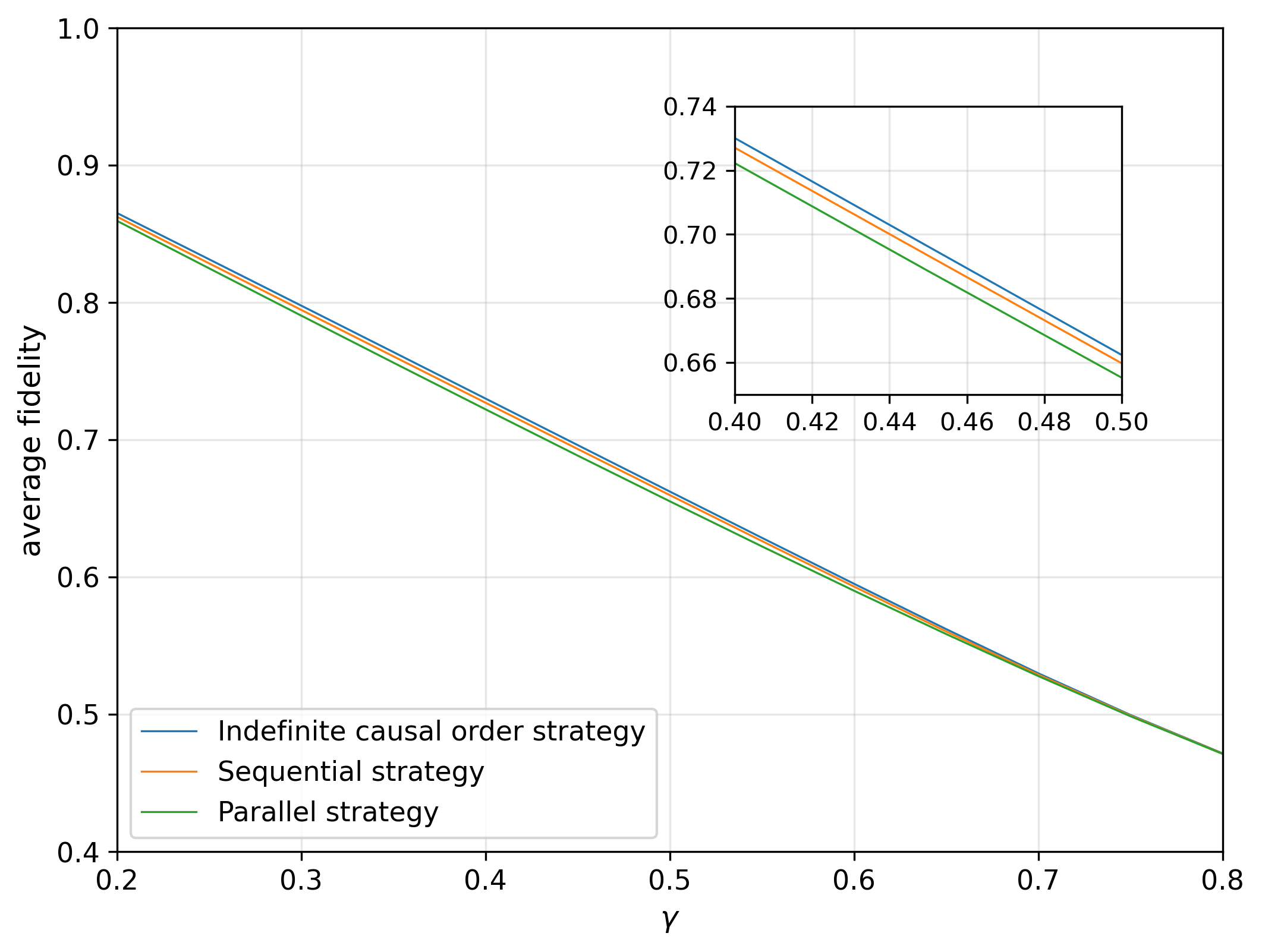
Remark 1 We note that this fundamental no-go result extends beyond the full unitary group to subsets exhibiting sufficient symmetry. For example, Theorem 1 applies to any unitary subset forming a unitary 3-design (e.g., the Clifford group), as the SDP performance evaluation involves terms up to the third tensor power of $U$. However, this structural obstruction vanishes when restricting target operations to less symmetric gate sets. For the specific gate set $\{X,Y,Z,I,H,S\}$, we conduct numerical experiments to compute the optimal average fidelity after purification across different strategies. The SDPs are solved by MATLAB [13] with the interpreters CVX [11, 10] and QETLAB [14]. We observe distinct performance gaps between parallel, sequential, and indefinite causal order strategies under depolarizing noise (see Fig. 4), indicating that the relaxation of symmetry constraints enables indefinite causal order strategies to substantially outperform conventional approaches, thereby indicating a potential regime where causal structures could yield advantages for mitigating error.

Figure 4: Optimal average fidelity for purification of $\{X,Y,Z,I,H,S\}$ against depolarizing noise under parallel, sequential, and indefinite causal order strategies.

IV Analytic Optimal Fidelity and Circuit Realization of the 3-Slot Architecture

Having established the fundamental impossibility of universal unitary purification with a 2-slot architecture, we now turn our attention to the next minimal realization: the 3-slot sequential strategy. Since a 2-slot strategy is strictly obstructed from providing any non-trivial fidelity gain, the 3-slot protocol represents the most resource-efficient architecture we can hope to employ.

In this section, we provide a fully analytical derivation of the optimal achievable fidelity for the 3-slot regime, alongside a concrete quantum circuit construction that explicitly realizes this theoretical maximum.

Figure 5: Schematic decomposition of the optimal quantum strategy. The rectangular blocks $V_{k}$ are the isometries. The system passes through the noisy channel depicted by the sequentially connected blocks $U$ and $\mathcal{N}_{\gamma}$, where $\mathcal{N}_{\gamma}$ is the depolarizing channel.

Theorem 2 (Optimal $3$-slot purification)

For all $\gamma\in(0,1)$, the depolarizing channel ${\cal N}_{\gamma}$ admits nontrivial $3$-slot sequential strategy satisfying the universal purification condition (4). Furthermore, the explicit value of the optimal fidelity for this unitary purification task is:

$$F_{\mathrm{opt}}^{*}(3;{\cal N}_{\gamma})=\frac{1}{24}(2-\gamma)\bigl[12+(8\sqrt{2}-9)\gamma+(3-8\sqrt{2})\gamma^{2}\bigr],$$ (13)

where $\gamma\in(0,1)$.

Proof sketch. Following a similar rationale to the first proof sketch, we begin by exploiting the unitary invariance inherent in the average fidelity objective. The symmetry of the underlying performance operator naturally translates to the optimization variable, allowing us to enforce invariance under the group action

$$\check{C}\;\mapsto\;U_{V,W}\,\check{C}\,U_{V,W}^{\dagger},\quad V,W\in\mathrm{SU}(2),$$ (14)

where $U_{V,W}=V_{P}\otimes V^{*\otimes 3}_{I^{3}}\otimes W^{*\otimes 3}_{O^{3}}\otimes W_{F}$. Analogously to Eq. (8), we twirl the Choi operator over the Haar measure to obtain a symmetrized strategy $\bar{C}$ that commutes with $U_{V,W}$ for all $V,W\in\mathrm{SU}(2)$, while preserving both validity and the achieved fidelity.

We further observe that the performance operator of the optimization objective is invariant under any permutation $\pi\in S_{3}$ of the slots $(I_{k},O_{k})$. Consequently, the optimal strategy must share this symmetry. Denoting the unitary representation of $\pi$ by $P_{\pi}$, we may therefore enforce $\bar{C}=P_{\pi}\,\bar{C}\,P_{\pi}^{\dagger}$ for all $\pi\in S_{3}$ without loss of generality.

Next, we apply the Clebsch-Gordan decomposition to the representation $(V,W)\mapsto V\otimes V^{*\otimes 3}\otimes W^{*\otimes 3}\otimes W$ of $\mathrm{SU}(2)\times\mathrm{SU}(2)$, which decomposes into nine irreducible sectors. By Schur’s lemma, the commutation relation $[\bar{C},U_{V,W}]=0$ forces $\bar{C}$ to be block-diagonal in the corresponding irreducible decomposition basis. Specifically, there exists a unitary $G\in\mathrm{SU}(256)$ such that

$$G^{\dagger}\,\bar{C}\,G=\bigoplus_{k=0}^{8}\bigl(H_{k}\otimes I_{d_{k}}\bigr),$$ (15)

where $H_{k}$ are positive semidefinite matrices and $d_{k}$ are the multiplicities of each sector.

This structure, combined with the $3$-slot sequential causality conditions and the $S_{3}$ symmetry, reduces the optimization to a low-dimensional SDP over the blocks $\{H_{k}\}$. To obtain a tractable upper bound, we further relax this SDP by retaining only a subset of the linear constraints, enlarging the feasible region. We then pass to the dual of this relaxed SDP and exhibit an explicit analytic dual-feasible solution. By weak duality, this immediately certifies that the optimal fidelity of any $3$-slot sequential strategy is at most the value in Eq. (13). To confirm achievability, we explicitly construct a $3$-slot sequential strategy that attains this value, which will be introduced in the following. Together, these two arguments establish $F_{\mathrm{opt}}^{*}(3;\mathcal{N}_{\gamma})$ as the exact optimal fidelity for $3$-slot unitary purification. $\square$

When $\gamma\in(0,1)$, the value of $F_{\mathrm{opt}}^{*}(3;{\cal N}_{\gamma})$ in Equation (13) is strictly greater than the fidelity achieved by a trivial strategy $F\!\left(J^{{\cal N}\circ{\cal U}},\,|U\rangle\hskip-2.27621pt\rangle\hskip-1.13809pt\langle\hskip-2.27621pt\langle U|\right)$, which is $1-\frac{3}{4}\gamma$. The details of this proof can be seen in Appendix B.

Finally, we briefly outline the schematic of our 3-slot purification protocol shown in Fig. 5. The protocol’s quantum strategy is realized by interleaving the noisy channel with a series of isometries $V_{k}$, the precise analytical matrices and circuit decompositions of which are detailed in Appendix C. The primary system qubit travels along the top wire, where it is sequentially subjected to the unitary $U$ followed by the depolarizing channel $\mathcal{N}_{\gamma}$ at each slot. To facilitate the purification, the isometries $V_{k}$ systematically introduce ancillary qubits (represented by the lower wires) to interact with the system. These ancillas essentially act as a quantum memory to process the information and absorb the errors. At the conclusion of the protocol, all ancillary systems are traced out, yielding the purified target state on the output system qubit.

V Discussion

We have proved that no nontrivial $2$-slot indefinite causal order strategy can universally purify the set of single-qubit unitaries under depolarizing noise. For the minimal nontrivial case of a 3-slot, we present an analytical derivation of the achievable fidelity. This derivation serves as a rigorous proof that the 3-slot sequential strategy strictly outperforms the standard trivial strategy on the unitary purification task. Furthermore, we provide a concrete circuit construction for this scenario.

While our current analysis primarily focuses on deterministic purification protocols, extending this framework to probabilistic cases represents a compelling direction for future research. Unlike the state case, the success probability in this context is governed by both the input noisy unitaries and the input state. Consequently, establishing a rigorous theoretical framework for probabilistic unitary purification and developing novel methodologies to analyze it remain important open problems. Furthermore, the scalability and composability of these quantum strategies remain intriguing open questions for future research. For instance, it is yet to be determined how the optimality of smaller strategies scales; specifically, whether concatenating two optimal $n$-slot strategies (e.g., $n=3$) inherently yields an optimal $2n$-slot strategy.

Appendix for ‘Distilling Unitary Operations: A No-Go Theorem and Minimal Realization’

Appendix A Proof of Theorem 1

We prove Theorem 1 by showing that for depolarizing noise with noise level $\gamma$, the optimal channel fidelity after purification is $1-\frac{3}{4}\gamma$, the same as that of a trivial purification.

Theorem S1

For the $2$-dimensional depolarizing noise channel ${\cal N}_{\gamma}$ with noise level $\gamma\in(0,1)$ and any $2$-slot ICO strategy, we have

$$\max_{{\cal C}\in\{ICO\}}\mathbb{E}_{U}C_{PI^{2}O^{2}F}*(J^{{\cal N}_{\gamma}}*|U\rangle\hskip-2.27621pt\rangle\hskip-1.13809pt\langle\hskip-2.27621pt\langle U|)^{\otimes 2}*(|U\rangle\hskip-2.27621pt\rangle\hskip-1.13809pt\langle\hskip-2.27621pt\langle U|)^{T}/4=1-\frac{3}{4}\gamma.$$ (S1)

Proof.

Firstly, we find

$$J^{{\cal N}_{\gamma}}*|U\rangle\hskip-2.27621pt\rangle\hskip-1.13809pt\langle\hskip-2.27621pt\langle U|=(1-\gamma)|U\rangle\hskip-2.27621pt\rangle\hskip-1.13809pt\langle\hskip-2.27621pt\langle U|+\frac{\gamma}{2}I_{4}$$ (S2)

and

$$J^{{\cal N}_{\gamma}}*|U\rangle\hskip-2.27621pt\rangle\hskip-1.13809pt\langle\hskip-2.27621pt\langle U|*(|U\rangle\hskip-2.27621pt\rangle\hskip-1.13809pt\langle\hskip-2.27621pt\langle U|)^{T}=4-3\gamma.$$ (S3)

Consider a $2$-slot general ICO strategy ${\cal C}$, as depicted in Fig. S1. $C_{PI^{2}O^{2}F}*(J^{{\cal N}_{\gamma}}*|U\rangle\hskip-2.27621pt\rangle\hskip-1.13809pt\langle\hskip-2.27621pt\langle U|)^{\otimes 2}$ is a qubit channel and have trace $d=2$, so (S1) is equivalent to

$$\max_{{\cal C}}\mathbb{E}_{U}C_{PI^{2}O^{2}F}*(J^{{\cal N}_{\gamma}}*|U\rangle\hskip-2.27621pt\rangle\hskip-1.13809pt\langle\hskip-2.27621pt\langle U|)^{\otimes 2}*(|U\rangle\hskip-2.27621pt\rangle\hskip-1.13809pt\langle\hskip-2.27621pt\langle U|)^{T}-\frac{4-3\gamma}{2}\operatorname{Tr}\left[C_{PI^{2}O^{2}F}*(J^{{\cal N}_{\gamma}}*|U\rangle\hskip-2.27621pt\rangle\hskip-1.13809pt\langle\hskip-2.27621pt\langle U|)^{\otimes 2})\right]=0.$$ (S4)

After rewriting the left hand of (S4) as

$$\max_{{\cal C}}\mathbb{E}_{U}C_{PI^{2}O^{2}F}*(J^{{\cal N}_{\gamma}}*|U\rangle\hskip-2.27621pt\rangle\hskip-1.13809pt\langle\hskip-2.27621pt\langle U|)^{\otimes 2}*(|U\rangle\hskip-2.27621pt\rangle\hskip-1.13809pt\langle\hskip-2.27621pt\langle U|)^{T}-\frac{4-3\gamma}{2}\operatorname{Tr}\left[C_{PI^{2}O^{2}F}*(J^{{\cal N}_{\gamma}}*|U\rangle\hskip-2.27621pt\rangle\hskip-1.13809pt\langle\hskip-2.27621pt\langle U|)^{\otimes 2})\right]$$ (S5)

$$= \max_{{\cal C}}\mathbb{E}_{U}C_{PI^{2}O^{2}F}*((1-\gamma)|U\rangle\hskip-2.27621pt\rangle\hskip-1.13809pt\langle\hskip-2.27621pt\langle U|+\frac{\gamma}{2}I_{4})^{\otimes 2}*((|U\rangle\hskip-2.27621pt\rangle\hskip-1.13809pt\langle\hskip-2.27621pt\langle U|)^{T}-\frac{4-3\gamma}{2}I_{4})$$ (S6)

$$= \max_{{\cal C}}\mathbb{E}_{U}\operatorname{Tr}\left[C_{PI^{2}O^{2}F}\cdot\left(\left((1-\gamma)|U\rangle\hskip-2.27621pt\rangle\hskip-1.13809pt\langle\hskip-2.27621pt\langle U|+\frac{\gamma}{2}I_{4}\right)^{T\otimes 2}_{I^{2}O^{2}}\otimes\left(|U\rangle\hskip-2.27621pt\rangle\hskip-1.13809pt\langle\hskip-2.27621pt\langle U|-\frac{4-3\gamma}{2}I_{4}\right)_{PF}\right)\right]$$ (S7)

$$= \max_{{\cal C}}\mathbb{E}_{U}\operatorname{Tr}\left[C_{PI^{2}O^{2}F}\cdot\left(\left((1-\gamma)|U^{*}\rangle\hskip-2.27621pt\rangle\hskip-1.13809pt\langle\hskip-2.27621pt\langle U^{*}|+\frac{\gamma}{2}I_{4}\right)^{\otimes 2}_{I^{2}O^{2}}\otimes\left(|U\rangle\hskip-2.27621pt\rangle\hskip-1.13809pt\langle\hskip-2.27621pt\langle U|-\frac{4-3\gamma}{2}I_{4}\right)_{PF}\right)\right]$$ (S8)

$$= \max_{{\cal C}}\operatorname{Tr}\left[C_{PI^{2}O^{2}F}\cdot\mathbb{E}_{U}\left[\left((1-\gamma)|U^{*}\rangle\hskip-2.27621pt\rangle\hskip-1.13809pt\langle\hskip-2.27621pt\langle U^{*}|+\frac{\gamma}{2}I_{4}\right)^{\otimes 2}_{I^{2}O^{2}}\otimes\left(|U\rangle\hskip-2.27621pt\rangle\hskip-1.13809pt\langle\hskip-2.27621pt\langle U|-\frac{4-3\gamma}{2}I_{4}\right)_{PF}\right]\right],$$ (S9)

we have another equivalent equation of (S1):

$$\max_{{\cal C}}\operatorname{Tr}\left[C_{PI^{2}O^{2}F}\cdot\mathbb{E}_{U}\left[\left((1-\gamma)|U^{*}\rangle\hskip-2.27621pt\rangle\hskip-1.13809pt\langle\hskip-2.27621pt\langle U^{*}|+\frac{\gamma}{2}I_{4}\right)^{\otimes 2}_{I^{2}O^{2}}\otimes\left(|U\rangle\hskip-2.27621pt\rangle\hskip-1.13809pt\langle\hskip-2.27621pt\langle U|-\frac{4-3\gamma}{2}I_{4}\right)_{PF}\right]\right]=0.$$ (S10)

Suppose that there exists a $2$-slot general strategy $\check{{\cal C}}$ satisfies

$$\operatorname{Tr}\left[\check{C}_{PI^{2}O^{2}F}\cdot\mathbb{E}_{U}\left[\left((1-\gamma)|U^{*}\rangle\hskip-2.27621pt\rangle\hskip-1.13809pt\langle\hskip-2.27621pt\langle U^{*}|+\frac{\gamma}{2}I_{4}\right)^{\otimes 2}_{I^{2}O^{2}}\otimes\left(|U\rangle\hskip-2.27621pt\rangle\hskip-1.13809pt\langle\hskip-2.27621pt\langle U|-\frac{4-3\gamma}{2}I_{4}\right)_{PF}\right]\right]>0,$$ (S11)

considering for any $V,W\in\operatorname{SU}(2)$,

$$\left[V_{P}\otimes V^{*\otimes 2}_{I_{1}I_{2}}\otimes W^{*\otimes 2}_{O_{1}O_{2}}\otimes W_{F},\mathbb{E}_{U}\left[\left((1-\gamma)|U^{*}\rangle\hskip-2.27621pt\rangle\hskip-1.13809pt\langle\hskip-2.27621pt\langle U^{*}|+\frac{\gamma}{2}I_{4}\right)^{\otimes 2}_{I^{2}O^{2}}\otimes\left(|U\rangle\hskip-2.27621pt\rangle\hskip-1.13809pt\langle\hskip-2.27621pt\langle U|-\frac{4-3\gamma}{2}I_{4}\right)_{PF}\right]\right]=0,$$ (S12)

we find (S11) still holds after replacing $\check{C}_{PI^{2}O^{2}F}$ with

$$(V_{P}\otimes V^{*\otimes 2}_{I_{1}I_{2}}\otimes W^{*\otimes 2}_{O_{1}O_{2}}\otimes W_{F})\cdot\check{C}_{PI^{2}O^{2}F}\cdot(V_{P}^{\dagger}\otimes V^{T\otimes 2}_{I_{1}I_{2}}\otimes W^{T\otimes 2}_{O_{1}O_{2}}\otimes W^{\dagger}_{F})\text{ for any }V,W\in\operatorname{SU}(2)$$ (S13)

or their expectation

$$\bar{C}_{PI^{2}O^{2}F}=\mathbb{E}_{V,W}(V_{P}\otimes V^{*\otimes 2}_{I_{1}I_{2}}\otimes W^{*\otimes 2}_{O_{1}O_{2}}\otimes W_{F})\cdot\check{C}_{PI^{2}O^{2}F}\cdot(V_{P}^{\dagger}\otimes V^{T\otimes 2}_{I_{1}I_{2}}\otimes W^{T\otimes 2}_{O_{1}O_{2}}\otimes W^{\dagger}_{F}).$$ (S14)

Thus we have obtained $\bar{C}_{PI^{2}O^{2}F}$ satisfies

$$\begin{cases}\operatorname{Tr}\left[\bar{C}_{PI^{2}O^{2}F}\cdot\mathbb{E}_{U}\left[\left((1-\gamma)|U^{*}\rangle\hskip-2.27621pt\rangle\hskip-1.13809pt\langle\hskip-2.27621pt\langle U^{*}|+\frac{\gamma}{2}I_{4}\right)^{\otimes 2}_{I^{2}O^{2}}\otimes\left(|U\rangle\hskip-2.27621pt\rangle\hskip-1.13809pt\langle\hskip-2.27621pt\langle U|-\frac{4-3\gamma}{2}I_{4}\right)_{PF}\right]\right]>0\\ \forall\,V,W\in\operatorname{SU}(2),\left[V_{P}\otimes V^{*\otimes 2}_{I_{1}I_{2}}\otimes W^{*\otimes 2}_{O_{1}O_{2}}\otimes W_{F},\bar{C}_{PI^{2}O^{2}F}\right]=0.\end{cases}$$ (S15)

By the irreducible representation decomposition of

$$\operatorname{SU}(2)\rightarrow\operatorname{SU}(8)\mathrel{\mathop{\mathchar 12346\relax}}\ U\mapsto U^{*\otimes 2}\otimes U=2U\oplus f_{4}(U),$$ (S16)

we have

$$\exists\,G\in\operatorname{SU}(8),\ s.t.\ \forall\,U\in\operatorname{SU}(2),\ G(U^{*\otimes 2}\otimes U)G^{\dagger}=\begin{pmatrix}I_{2}\otimes U\\ &f_{4}(U)\end{pmatrix},$$ (S17)

where $f_{4}$ is a $4$-dimensional irreducible representation of $\operatorname{SU}(2)$. Moreover by the irreducible representation decomposition of $\operatorname{SU}(2)\times\operatorname{SU}(2)\rightarrow\operatorname{SU}(64)$:

$$(V,W)\mapsto V\otimes V^{*\otimes 2}\otimes W^{*\otimes 2}\otimes W=4V\otimes W\oplus 2f_{4}(V)\otimes W\oplus 2f_{4}(W)\otimes V\oplus f_{4}(V)\otimes f_{4}(W),$$ (S18)

The following computation is based on a specific $G\in\operatorname{SU}(64)$. Applying a permutation matrix $P$ on the left and $P^{T}$ on the right could induce a permutation of the tensor factors, mapping $V\otimes V^{*\otimes 2}\otimes W^{*\otimes 2}\otimes W\mapsto V\otimes(V\otimes W)^{*\otimes 2}\otimes W$. We then set $\tilde{G}=GP$ , s.t. $\forall\,V,W\in\operatorname{SU}(2)$,

$$\tilde{G}\cdot(V\otimes V^{*\otimes 2}\otimes W^{*\otimes 2}\otimes W)\cdot\tilde{G}^{\dagger}$$ (S19a)

$$= \begin{pmatrix}I_{4}\otimes V\otimes W\\ &I_{2}\otimes V\otimes f_{4}(W)\\ &&I_{2}\otimes W\otimes f_{4}(V)\\ &&&f_{4}(V)\otimes f_{4}(W)\end{pmatrix},$$ (S19b)

Since $\bar{C}_{PI^{2}O^{2}F}$ is always commutative with $V_{P}\otimes V^{*\otimes 2}_{I_{1}I_{2}}\otimes W^{*\otimes 2}_{O_{1}O_{2}}\otimes W_{F}$ for any $V,W\in\operatorname{SU}(2)$, by Schur’s lemma, we have $\bar{C}_{PI^{2}O^{2}F}$ is of form

$$\tilde{G}\cdot\bar{C}_{PI^{2}O^{2}F}\cdot\tilde{G}^{\dagger}=\begin{pmatrix}H_{0}\otimes I_{4}\\ &H_{1}\otimes I_{8}\\ &&H_{2}\otimes I_{8}\\ &&&h_{3}I_{16}\end{pmatrix}=\begin{pmatrix}H_{0}\\ &H_{1}\otimes I_{2}\\ &&H_{2}\otimes I_{2}\\ &&&h_{3}I_{4}\end{pmatrix}\otimes I_{4},$$ (S20)

where $H_{0}=\{H_{0jk}\}_{jk}\in\mathbb{C}^{4\times 4}$, $H_{1}=\{H_{1jk}\}_{jk},H_{2}=\{H_{2jk}\}_{jk}\in\mathbb{C}^{2\times 2}$, $h_{3}\in\mathbb{C}$. After denoting $\operatorname{Tr}_{d}$ as the partial trace on the last $d$-dimensional system and

$$\operatorname{Tr}_{4}\left[\tilde{G}\cdot\mathbb{E}_{U}\left[\left((1-\gamma)|U^{*}\rangle\hskip-2.27621pt\rangle\hskip-1.13809pt\langle\hskip-2.27621pt\langle U^{*}|+\frac{\gamma}{2}I_{4}\right)^{\otimes 2}_{I^{2}O^{2}}\otimes\left(|U\rangle\hskip-2.27621pt\rangle\hskip-1.13809pt\langle\hskip-2.27621pt\langle U|-\frac{4-3\gamma}{2}I_{4}\right)_{PF}\right]\cdot\tilde{G}^{\dagger}\right]\\ =\sum_{jk=0}^{3}|j\rangle\!\langle k|\otimes\Omega_{jk},$$ (S21)

we have

$$\operatorname{Tr}\left[\bar{C}_{PI^{2}O^{2}F}\cdot\mathbb{E}_{U}\left[\left((1-\gamma)|U^{*}\rangle\hskip-2.27621pt\rangle\hskip-1.13809pt\langle\hskip-2.27621pt\langle U^{*}|+\frac{\gamma}{2}I_{4}\right)^{\otimes 2}_{I^{2}O^{2}}\otimes\left(|U\rangle\hskip-2.27621pt\rangle\hskip-1.13809pt\langle\hskip-2.27621pt\langle U|-\frac{4-3\gamma}{2}I_{4}\right)_{PF}\right]\right]$$ (S22a)

$$= \operatorname{Tr}[H_{0}\Omega_{00}]+\operatorname{Tr}[H_{1}\operatorname{Tr}_{2}[\Omega_{11}]]+\operatorname{Tr}[H_{2}\operatorname{Tr}_{2}[\Omega_{22}]]+h_{3}\operatorname{Tr}[\Omega_{33}],$$ (S22b)

where

$$\Omega_{00} =\left(\begin{array}[]{cccc}-\frac{1}{6}(1-\gamma)\left(3(1-\gamma)^{2}+1\right)&-(1-\gamma)(2-\gamma)\\ -(1-\gamma)(2-\gamma)&-\frac{3}{2}(1-\gamma)\left(3(1-\gamma)^{2}+1\right)\\ &&-\frac{3}{2}\gamma^{3}+\frac{9}{2}\gamma^{2}-3\gamma&(1-\gamma)\gamma\\ &&(1-\gamma)\gamma&-\frac{3}{2}\gamma^{3}+\frac{9}{2}\gamma^{2}-3\gamma\\ \end{array}\right),$$ (S27)

$$\operatorname{Tr}_{2}[\Omega_{11}] =\operatorname{Tr}_{2}[\Omega_{22}]=\left(\begin{array}[]{cc}-\frac{1}{3}(1-\gamma)\left(3(1-\gamma)^{2}+13\right)\\ &-3(1-\gamma)(1-(1-\gamma)^{2})\\ \end{array}\right),$$ (S30)

$$\operatorname{Tr}[\Omega_{33}] =-\frac{2}{3}(1-\gamma)\left(3(1-\gamma)^{2}+7\right).$$ (S31)

Since $\bar{{\cal C}}$ is an indefinite causal order strategy, as depicted in Fig. S1. Specifically, $\bar{{\cal C}}$ is a valid ICO strategy if and only if its corresponding Choi operator $\bar{C}$ on the joint system $PI^{2}O^{2}F$ satisfies the following conditions:

$$\begin{cases}\bar{C}\geq 0\\ {}_{I_{1}O_{1}F}\bar{C}={}_{I_{1}O_{1}O_{2}F}\bar{C}\\ {}_{I_{2}O_{2}F}\bar{C}={}_{O_{1}I_{2}O_{2}F}\bar{C}\\ {}_{I^{2}O^{2}F}\bar{C}={}_{PI^{2}O^{2}F}\bar{C}\\ {}_{F}\bar{C}+{}_{O_{1}O_{2}F}\bar{C}={}_{O_{1}F}\bar{C}+{}_{O_{2}F}\bar{C}\\ \operatorname{Tr}[\bar{C}]=8\end{cases}$$ (S32)

which is equivalent to

$$\begin{cases}H_{0},H_{1},H_{2},h_{3}\geq 0\\ H_{100}=\frac{1}{2}\left(3H_{033}-H_{000}\right)\\ H_{101}=\frac{1}{2}\left(3H_{013}^{*}-H_{002}\right)\\ H_{111}=\frac{1}{2}\left(3H_{011}-H_{022}\right)\\ H_{211}=\frac{1}{4}\left(-2H_{011}-2H_{033}+1\right)\\ h_{3}=\frac{1}{8}\left(-6H_{011}-6H_{033}-4H_{200}+3\right)\end{cases}$$ (S33)

we have the following SDP

$$\max\; \operatorname{Tr}\left[\bar{C}_{PI^{2}O^{2}F}\cdot\mathbb{E}_{U}\left[\left((1-\gamma)|U^{*}\rangle\hskip-2.27621pt\rangle\hskip-1.13809pt\langle\hskip-2.27621pt\langle U^{*}|+\frac{\gamma}{2}I_{4}\right)^{\otimes 2}_{I^{2}O^{2}}\otimes\left(|U\rangle\hskip-2.27621pt\rangle\hskip-1.13809pt\langle\hskip-2.27621pt\langle U|-\frac{4-3\gamma}{2}I_{4}\right)_{PF}\right]\right]$$ (S34a)

s.t. $$\tilde{G}\cdot\bar{C}_{PI^{2}O^{2}F}\cdot\tilde{G}^{\dagger}=\begin{pmatrix}H_{0}\\ &H_{1}\otimes I_{2}\\ &&H_{2}\otimes I_{2}\\ &&&h_{3}I_{4}\end{pmatrix}\otimes I_{4};$$ (S34b)

$$\bar{C}_{PI^{2}O^{2}F}\in\{ICO\}$$ (S34c)

is equivalent to

$$\max\; \operatorname{Tr}[H_{0}\Omega_{00}]+\operatorname{Tr}[H_{1}\operatorname{Tr}_{2}[\Omega_{11}]]+\operatorname{Tr}[H_{2}\operatorname{Tr}_{2}[\Omega_{22}]]+h_{3}\operatorname{Tr}[\Omega_{33}]$$ (S35a)

s.t. $$H_{0},H_{1},H_{2},h_{3}\geq 0$$ (S35b)

$$H_{100}=\frac{1}{2}\left(3H_{033}-H_{000}\right)$$ (S35c)

$$H_{101}=\frac{1}{2}\left(3H_{013}^{*}-H_{002}\right)$$ (S35d)

$$H_{111}=\frac{1}{2}\left(3H_{011}-H_{022}\right)$$ (S35e)

$$H_{211}=\frac{1}{4}\left(-2H_{011}-2H_{033}+1\right)$$ (S35f)

$$h_{3}=\frac{1}{8}\left(-6H_{011}-6H_{033}-4H_{200}+3\right)$$ (S35g)

and also

$$\max\; \operatorname{Tr}\left[\begin{pmatrix}H_{000}&H_{001}\\ H_{001}^{*}&H_{011}\end{pmatrix}\begin{pmatrix}2(1-\gamma)&-(1-\gamma)(2-\gamma)\\ -(1-\gamma)(2-\gamma)&-(1-\gamma)\end{pmatrix}\right]+$$ (S36a)

$$\operatorname{Tr}\left[\begin{pmatrix}H_{022}&H_{023}\\ H_{023}^{*}&H_{033}\end{pmatrix}\begin{pmatrix}0&(1-\gamma)\gamma\\ (1-\gamma)\gamma&-3(1-\gamma)\end{pmatrix}\right]-\frac{1}{2}(1-\gamma)\left(4H_{200}+5\right)$$ (S36b)

s.t. $$H_{0}\geq 0$$ (S36c)

$$\begin{pmatrix}\frac{1}{2}\left(3H_{033}-H_{000}\right)&\frac{1}{2}\left(3H_{013}^{*}-H_{002}\right)\\ \frac{1}{2}\left(3H_{013}^{*}-H_{002}\right)^{*}&\frac{1}{2}\left(3H_{011}-H_{022}\right)\end{pmatrix}\geq 0$$ (S36d)

$$\begin{pmatrix}H_{200}&H_{201}\\ H_{201}^{*}&\frac{1}{4}\left(-2H_{011}-2H_{033}+1\right)\end{pmatrix}\geq 0$$ (S36e)

$$-6H_{011}-6H_{033}-4H_{200}+3\geq 0.$$ (S36f)

For any optimal solution of (S36), maintaining the values of $\{H_{000},H_{001},H_{011},H_{022},H_{023},H_{033},H_{200}\}$ and replacing the values of any other variables (that is, in $\{H_{002},H_{003},H_{012},H_{013},H_{201}\}$) by $0$, we will obtain another optimal solution because it is an easily checked feasible solution with the same objective function value with the optimal solution of the origin. The new optimal solution could be described by the following SDP:

$$\max\; \operatorname{Tr}\left[\begin{pmatrix}H_{000}&H_{001}\\ H_{001}^{*}&H_{011}\end{pmatrix}\begin{pmatrix}2(1-\gamma)&-(1-\gamma)(2-\gamma)\\ -(1-\gamma)(2-\gamma)&-(1-\gamma)\\ \end{pmatrix}\right]+$$ (S37a)

$$\operatorname{Tr}\left[\begin{pmatrix}H_{022}&H_{023}\\ H_{023}^{*}&H_{033}\end{pmatrix}\begin{pmatrix}0&(1-\gamma)\gamma\\ (1-\gamma)\gamma&-3(1-\gamma)\\ \end{pmatrix}\right]-\frac{1}{2}(1-\gamma)\left(4H_{200}+5\right)$$ (S37b)

s.t. $$\begin{pmatrix}H_{000}&H_{001}\\ H_{001}^{*}&H_{011}\end{pmatrix},\begin{pmatrix}H_{022}&H_{023}\\ H_{023}^{*}&H_{033}\end{pmatrix}\geq 0$$ (S37c)

$$3H_{033}-H_{000},3H_{011}-H_{022}\geq 0$$ (S37d)

$$H_{200},-2H_{011}-2H_{033}+1\geq 0$$ (S37e)

$$-6H_{011}-6H_{033}-4H_{200}+3\geq 0.$$ (S37f)

Firstly, we could find the above SDP reaches its maximum only if $H_{200}=0$, and simplify it as

$$\max\; \operatorname{Tr}\left[\left(\begin{array}[]{cc}H_{000}&H_{001}\\ H_{001}^{*}&H_{011}\end{array}\right)\left(\begin{array}[]{cc}2(1-\gamma)&-(1-\gamma)(2-\gamma)\\ -(1-\gamma)(2-\gamma)&-(1-\gamma)\\ \end{array}\right)\right]+$$ (S38e)

$$\operatorname{Tr}\left[\left(\begin{array}[]{cc}H_{022}&H_{023}\\ H_{023}^{*}&H_{033}\end{array}\right)\left(\begin{array}[]{cc}0&(1-\gamma)\gamma\\ (1-\gamma)\gamma&-3(1-\gamma)\\ \end{array}\right)\right]-\frac{5}{2}(1-\gamma)$$ (S38j)

s.t. $$\left(\begin{array}[]{cc}H_{000}&H_{001}\\ H_{001}^{*}&H_{011}\end{array}\right),\left(\begin{array}[]{cc}H_{022}&H_{023}\\ H_{023}^{*}&H_{033}\end{array}\right)\geq 0$$ (S38o)

$$3H_{033}-H_{000},3H_{011}-H_{022},-2H_{011}-2H_{033}+1\geq 0.$$ (S38p)

Secondly, due to the constraints of (S38), we have at least $H_{000},\,H_{011},\,H_{022},\,H_{033}\geq 0$ and $H_{011}+H_{033}\leq\tfrac{1}{2}$, hence $H_{011},\,H_{033}\in[0,\tfrac{1}{2}]$. By the remaining constraints, we further obtain $H_{000},\,H_{022}\in[0,\tfrac{3}{2}]$. Moreover, the positive semidefiniteness conditions imposed by the constraints imply that the feasible region of the SDP is a bounded closed set, and the objective function is non-constant; therefore, any optimal solution must be attained on the boundary. It follows that $|H_{001}|^{2}=H_{000}\cdot H_{011}.$ Since we seek the maximum value and $-(1-\gamma)(2-\gamma)<0$ for $\gamma\in(0,1)$, we choose $H_{001}=-\sqrt{H_{000}\cdot H_{011}}.$ By analogous reasoning, $H_{023}=\sqrt{H_{022}H_{033}}$, and the SDP can be simplified as

$$\max\; \operatorname{Tr}\left[\left(\begin{array}[]{cc}H_{000}&\sqrt{H_{000}H_{011}}\\ \sqrt{H_{000}H_{011}}&H_{011}\end{array}\right)\left(\begin{array}[]{cc}2(1-\gamma)&(1-\gamma)(2-\gamma)\\ (1-\gamma)(2-\gamma)&-(1-\gamma)\\ \end{array}\right)\right]+$$ (S39e)

$$\operatorname{Tr}\left[\left(\begin{array}[]{cc}H_{022}&\sqrt{H_{022}H_{033}}\\ \sqrt{H_{022}H_{033}}&H_{033}\end{array}\right)\left(\begin{array}[]{cc}0&(1-\gamma)\gamma\\ (1-\gamma)\gamma&-3(1-\gamma)\\ \end{array}\right)\right]-\frac{5}{2}(1-\gamma)$$ (S39j)

s.t. $$H_{000},H_{011},H_{022},H_{033}\geq 0$$ (S39k)

$$3H_{033}-H_{000},3H_{011}-H_{022},-2H_{011}-2H_{033}+1\geq 0.$$ (S39l)

Thirdly, we could find the above programming reaches its maximum only if $H_{000}=3H_{033}$,$H_{022}=3H_{011}$, and simplified it as

$$\max\; \operatorname{Tr}\left[\left(\begin{array}[]{cc}H_{011}&\sqrt{H_{011}H_{033}}\\ \sqrt{H_{011}H_{033}}&H_{033}\\ \end{array}\right)\left(\begin{array}[]{cc}-(1-\gamma)&2\sqrt{3}(1-\gamma)\\ 2\sqrt{3}(1-\gamma)&3(1-\gamma)\\ \end{array}\right)\right]-\frac{5}{2}(1-\gamma)$$ (S40e)

s.t. $$H_{011},H_{033},-2H_{011}-2H_{033}+1\geq 0.$$ (S40f)

Notice that we can rewrite the above SDP as:

$$\max\; \left(\begin{array}[]{cc}\sqrt{H_{011}}&\sqrt{H_{033}}\end{array}\right)\left(\begin{array}[]{cc}-(1-\gamma)&2\sqrt{3}(1-\gamma)\\ 2\sqrt{3}(1-\gamma)&3(1-\gamma)\\ \end{array}\right)\left(\begin{array}[]{cc}\sqrt{H_{011}}\\ \sqrt{H_{033}}\\ \end{array}\right)-\frac{5}{2}(1-\gamma)$$ (S41f)

s.t. $$H_{011},H_{033},-2H_{011}-2H_{033}+1\geq 0.$$ (S41g)

Since the maximal eigenvalue of $\left(\begin{array}[]{cc}-(1-\gamma)&2\sqrt{3}(1-\gamma)\\ 2\sqrt{3}(1-\gamma)&3(1-\gamma)\\ \end{array}\right)$ is $5(1-\gamma)$ with eigenstate $(\frac{1}{2},\frac{\sqrt{3}}{2})^{T}$, (S41) reaches is maximum $0$ if and only if $(\sqrt{H_{011}},\sqrt{H_{033}})=\frac{1}{\sqrt{2}}(\frac{1}{2},\frac{\sqrt{3}}{2})$.

As a result, the optimal value of SDP (S34) is $0$, which contradicts the existence of $\bar{{\cal C}}$ in (S15). Thus, the origin assumption (S11) is false, which leads to

$$\max_{{\cal C}\in\{ICO\}}\mathbb{E}_{U}C_{PI^{2}O^{2}F}*(J^{{\cal N}_{\gamma}}*|U\rangle\hskip-2.27621pt\rangle\hskip-1.13809pt\langle\hskip-2.27621pt\langle U|)^{\otimes 2}*|U\rangle\hskip-2.27621pt\rangle\hskip-1.13809pt\langle\hskip-2.27621pt\langle U|^{T}/4\leq 1-\frac{3}{4}\gamma.$$ (S42)

$\sqcap$$\sqcup$

Figure S1: Illustration of the $2$-slot indefinite causal order strategy structure ${\cal C}$.

Appendix B Proof of Theorem 2

Theorem S2 (Optimal $3$-slot purification)

For the depolarizing channel ${\cal N}_{\gamma}$ with noise level $\gamma\in(0,1)$, we construct an optimal $3$-slot sequential strategy with analytical optimal average fidelity

$$F_{\mathrm{opt}}^{*}(3;{\cal N}_{\gamma})=\frac{1}{24}(2-\gamma)(12+(8\sqrt{2}-9)\gamma+(3-8\sqrt{2})\gamma^{2}),$$ (S43)

Furthermore, it satisfies the universal purification condition (4).

Proof.

First, we prove the optimality of Eq. (S43). Suppose that there exists a $3$-slot general strategy $\check{{\cal C}}$ satisfies

$$\operatorname{Tr}\left[\check{C}_{PI^{3}O^{3}F}\cdot\mathbb{E}_{U}\left[\left((1-\gamma)|U^{*}\rangle\hskip-2.27621pt\rangle\hskip-1.13809pt\langle\hskip-2.27621pt\langle U^{*}|+\frac{\gamma}{2}I_{4}\right)^{\otimes 3}_{I^{3}O^{3}}\otimes\left(|U\rangle\hskip-2.27621pt\rangle\hskip-1.13809pt\langle\hskip-2.27621pt\langle U|\right)_{PF}\right]\right]=F,$$ (S44)

for some $F\in[0,1]$. Considering any $V,W\in\operatorname{SU}(2)$ fulfilling the following commutativity:

$$\left[V_{P}\otimes V^{*\otimes 3}_{I_{1}I_{2}I_{3}}\otimes W^{*\otimes 3}_{O_{1}O_{2}O_{3}}\otimes W_{F},\mathbb{E}_{U}\left[\left((1-\gamma)|U^{*}\rangle\hskip-2.27621pt\rangle\hskip-1.13809pt\langle\hskip-2.27621pt\langle U^{*}|+\frac{\gamma}{2}I_{4}\right)^{\otimes 3}_{I^{3}O^{3}}\otimes\left(|U\rangle\hskip-2.27621pt\rangle\hskip-1.13809pt\langle\hskip-2.27621pt\langle U|\right)_{PF}\right]\right]=0,$$ (S45)

we find (S44) still holds after replacing $\check{C}_{PI^{3}O^{3}F}$ with

$$(V_{P}\otimes V^{*\otimes 3}_{I_{1}I_{2}I_{3}}\otimes W^{*\otimes 3}_{O_{1}O_{2}O_{3}}\otimes W_{F})\cdot\check{C}_{PI^{3}O^{3}F}\cdot(V_{P}^{\dagger}\otimes V^{T\otimes 3}_{I_{1}I_{2}I_{3}}\otimes W^{T\otimes 3}_{O_{1}O_{2}O_{3}}\otimes W^{\dagger}_{F})\text{ for any }V,W\in\operatorname{SU}(2)$$ (S46)

and so does its expectation

$$\bar{C}_{PI^{3}O^{3}F}=\mathbb{E}_{V,W}\left[(V_{P}\otimes V^{*\otimes 3}_{I_{1}I_{2}I_{3}}\otimes W^{*\otimes 3}_{O_{1}O_{2}O_{3}}\otimes W_{F})\cdot\check{C}_{PI^{3}O^{3}F}\cdot(V_{P}^{\dagger}\otimes V^{T\otimes 3}_{I_{1}I_{2}I_{3}}\otimes W^{T\otimes 3}_{O_{1}O_{2}O_{3}}\otimes W^{\dagger}_{F})\right].$$ (S47)

Thus we have obtained $\bar{C}_{PI^{3}O^{3}F}$ satisfies

$$\begin{cases}\operatorname{Tr}\left[\bar{C}_{PI^{3}O^{3}F}\cdot\mathbb{E}_{U}\left[\left((1-\gamma)|U^{*}\rangle\hskip-2.27621pt\rangle\hskip-1.13809pt\langle\hskip-2.27621pt\langle U^{*}|+\frac{\gamma}{2}I_{4}\right)^{\otimes 3}_{I^{3}O^{3}}\otimes\left(|U\rangle\hskip-2.27621pt\rangle\hskip-1.13809pt\langle\hskip-2.27621pt\langle U|\right)_{PF}\right]\right]>0\\ \forall\,V,W\in\operatorname{SU}(2),\left[V_{P}\otimes V^{*\otimes 3}_{I_{1}I_{2}I_{3}}\otimes W^{*\otimes 3}_{O_{1}O_{2}O_{3}}\otimes W_{F},\bar{C}_{PI^{3}O^{3}F}\right]=0.\end{cases}$$ (S48)

By the irreducible representation decomposition of

$$\operatorname{SU}(2)\rightarrow\operatorname{SU}(16)\mathrel{\mathop{\mathchar 12346\relax}}\ U\mapsto U^{*\otimes 3}\otimes U=2f_{1}(U)\oplus 3f_{3}(U)\oplus f_{5}(U),$$ (S49)

we have

$$\exists\,G\in\operatorname{SU}(16),\ s.t.\ \forall\,U\in\operatorname{SU}(2),\ G^{\dagger}(U^{*\otimes 3}\otimes U)G=\begin{pmatrix}I_{2}\otimes f_{1}(U)\\ &I_{3}\otimes f_{3}(U)\\ &&f_{5}(U)\end{pmatrix},$$ (S50)

where $f_{d}$ is the $d$-dimensional irreducible representation of $\operatorname{SU}(2)$. Moreover by the irreducible representation decomposition of $\operatorname{SU}(2)\times\operatorname{SU}(2)\rightarrow\operatorname{SU}(256)$:

$$(V,W)\mapsto V\otimes V^{*\otimes 3}\otimes W^{*\otimes 3}\otimes W= 4f_{1}(V)\otimes f_{1}(W)\oplus 6f_{1}(V)\otimes f_{3}(W)\oplus 2f_{1}(V)\otimes f_{5}(W)$$ (S51)

$$\oplus 6f_{3}(V)\otimes f_{1}(W)\oplus 9f_{3}(V)\otimes f_{3}(W)\oplus 3f_{3}(V)\otimes f_{5}(W)$$

$$\oplus 2f_{5}(V)\otimes f_{1}(W)\oplus 3f_{5}(V)\otimes f_{3}(W)\oplus f_{5}(V)\otimes f_{5}(W),$$

By employing the Clebsch-Gordan decomposition, we construct a specific unitary $G\in\operatorname{SU}(256)$(provided in our GitHub repository) such that for any $V,W\in\operatorname{SU}(2)$,

$$G^{\dagger}\cdot(V\otimes V^{*\otimes 3}\otimes W^{*\otimes 3}\otimes W)\cdot G$$ (S52a)

$$= \resizebox{483.84706pt}{}{$\begin{pmatrix}I_{4}\otimes f_{1}(V)\otimes f_{1}(W)\\ &I_{6}\otimes f_{1}(V)\otimes f_{3}(W)\\ &&I_{2}\otimes f_{1}(V)\otimes f_{5}(W)\\ &&&I_{6}\otimes f_{3}(V)\otimes f_{1}(W)\\ &&&&I_{9}\otimes f_{3}(V)\otimes f_{3}(W)\\ &&&&&I_{3}\otimes f_{3}(V)\otimes f_{5}(W)\\ &&&&&&I_{2}\otimes f_{5}(V)\otimes f_{1}(W)\\ &&&&&&&I_{3}\otimes f_{5}(V)\otimes f_{3}(W)\\ &&&&&&&&f_{5}(V)\otimes f_{5}(W)\end{pmatrix}$}.$$ (S52b)

Since $\bar{C}_{PI^{3}O^{3}F}$ is always commutative with $V_{P}\otimes V^{*\otimes 3}_{I_{1}I_{2}I_{3}}\otimes W^{*\otimes 3}_{O_{1}O_{2}O_{3}}\otimes W_{F}$ for any $V,W\in\operatorname{SU}(2)$, by Schur’s lemma, we have $\bar{C}_{PI^{3}O^{3}F}$ is of form

$$G^{\dagger}\cdot\bar{C}_{PI^{2}O^{2}F}\cdot G=\begin{pmatrix}H_{0}\otimes I_{1}\\ &H_{1}\otimes I_{3}\\ &&H_{2}\otimes I_{5}\\ &&&H_{3}\otimes I_{3}\\ &&&&H_{4}\otimes I_{9}\\ &&&&&H_{5}\otimes I_{15}\\ &&&&&&H_{6}\otimes I_{5}\\ &&&&&&&H_{7}\otimes I_{15}\\ &&&&&&&&h_{8}I_{25}\end{pmatrix},$$ (S53)

where $H_{0}=\{H_{0jk}\}_{jk}\in\mathbb{C}^{4\times 4}$, $H_{1}=\{H_{1jk}\}_{jk},H_{3}=\{H_{3jk}\}_{jk}\in\mathbb{C}^{6\times 6}$, $H_{2}=\{H_{2jk}\}_{jk},H_{6}=\{H_{6jk}\}_{jk}\in\mathbb{C}^{2\times 2}$, $H_{4}=\{H_{4jk}\}_{jk}\in\mathbb{C}^{9\times 9}$, $H_{5}=\{H_{5jk}\}_{jk},H_{7}=\{H_{7jk}\}_{jk}\in\mathbb{C}^{3\times 3}$, and $h_{8}\in\mathbb{C}$.

Furthermore, the performance operator in our objective function, $\operatorname{Tr}(\Omega\bar{C}_{PI^{3}O^{3}F})$, where

$$\Omega=\mathbb{E}_{U}\left[\left((1-\gamma)|U^{*}\rangle\hskip-2.27621pt\rangle\hskip-1.13809pt\langle\hskip-2.27621pt\langle U^{*}|+\frac{\gamma}{2}I_{4}\right)^{\otimes 3}_{I^{3}O^{3}}\otimes\left(|U\rangle\hskip-2.27621pt\rangle\hskip-1.13809pt\langle\hskip-2.27621pt\langle U|\right)_{PF}\right],$$ (S54)

is completely invariant under any permutation of the three physical slots $(I_{1},O_{1})$, $(I_{2},O_{2})$, and $(I_{3},O_{3})$. Let $P_{\pi}$ denote the unitary representation of a permutation $\pi\in S_{3}$ acting on these physical slots, such that $P_{\pi}^{\dagger}\Omega P_{\pi}=\Omega$. Because of this objective symmetry, we can safely enforce an exact $S_{3}$ permutation symmetry on the physical strategy itself, restricting the search to $\bar{C}_{PI^{3}O^{3}F}=P_{\pi}\bar{C}_{PI^{3}O^{3}F}P_{\pi}^{\dagger}$, without altering the globally optimal fidelity.

Since the symmetric group $S_{3}$ is generated by two transpositions—swapping the first and second slots ($P_{12}$) and swapping the second and third slots ($P_{23}$)—we simply extract the homogeneous linear constraints directly in the physical basis:

$$\bar{C}_{PI^{3}O^{3}F}-P_{12}\bar{C}_{PI^{3}O^{3}F}P_{12}^{\dagger} =0,$$ (S55)

$$\bar{C}_{PI^{3}O^{3}F}-P_{23}\bar{C}_{PI^{3}O^{3}F}P_{23}^{\dagger} =0.$$ (S56)

Taking the causality conditions of the $3$-slot sequential strategy $\bar{{\cal C}}$ together with the $S_{3}$ symmetry conditions derived above, one could assume the Choi operator $\bar{C}$ satisfy:

$$\begin{cases}\bar{C}\geq 0\\ {}_{F}\bar{C}={}_{O_{3}F}\bar{C}\\ {}_{I_{3}O_{3}F}\bar{C}={}_{O_{2}I_{3}O_{3}F}\bar{C}\\ {}_{I_{2}O_{2}I_{3}O_{3}F}\bar{C}={}_{O_{1}I_{2}O_{2}I_{3}O_{3}F}\bar{C}\\ {}_{I^{3}O^{3}F}\bar{C}={}_{PI^{3}O^{3}F}\bar{C}\\ \operatorname{Tr}[\bar{C}]=16\\ \bar{C}_{PI^{3}O^{3}F}-P_{12}\bar{C}_{PI^{3}O^{3}F}P_{12}^{\dagger}=0\\ \bar{C}_{PI^{3}O^{3}F}-P_{23}\bar{C}_{PI^{3}O^{3}F}P_{23}^{\dagger}=0\end{cases}$$ (S57)

which is equivalent to

$$\begin{cases}H_{0},H_{1},\dots,h_{8}\geq 0\\ \mathcal{L}_{\text{sym \& causal}}(H_{0},H_{1},\dots,h_{8})=0\end{cases}$$ (S58)

where $\mathcal{L}$ represents the exact algebraic linear constraints. Specifically, the constraint system $\mathcal{L}$ consists of 196 variables and 171 equality constraints, leaving 25 unconstrained degrees of freedom. The computation of these linear constraints and the subsequent reduction process used in the following proof are available in our GitHub repository. Because these remaining free variables are purely redundant, assigning specific values to them does not affect the feasibility or the outcome of the SDP. By fixing some of these redundant variables, we obtain the following SDP:

$$\max\; \operatorname{Tr}\left[\bar{C}_{PI^{3}O^{3}F}\cdot\mathbb{E}_{U}\left[\left((1-\gamma)|U^{*}\rangle\hskip-2.27621pt\rangle\hskip-1.13809pt\langle\hskip-2.27621pt\langle U^{*}|+\frac{\gamma}{2}I_{4}\right)^{\otimes 3}_{I^{3}O^{3}}\otimes\left(|U\rangle\hskip-2.27621pt\rangle\hskip-1.13809pt\langle\hskip-2.27621pt\langle U|\right)_{PF}\right]\right]$$ (S59a)

s.t. $$G^{\dagger}\cdot\bar{C}_{PI^{3}O^{3}F}\cdot G=\bigoplus_{k=0}^{8}\left(H_{k}\otimes I_{d_{k}}\right);$$ (S59b)

$$\bar{C}_{PI^{3}O^{3}F}\in\{\text{Sequential strategy}\}$$ (S59c)

$$\bar{C}_{PI^{3}O^{3}F}-P_{12}\bar{C}_{PI^{3}O^{3}F}P_{12}^{\dagger}=0$$ (S59d)

$$\bar{C}_{PI^{3}O^{3}F}-P_{23}\bar{C}_{PI^{3}O^{3}F}P_{23}^{\dagger}=0$$ (S59e)

$$\text{Re}(H_{211})=\text{Re}(H_{455})=\text{Re}(H_{488})=\dots=0\qquad\text{(redundant variable assignments)}$$ (S59f)

If we take linear combinations of some constraints within $\mathcal{L}_{\text{sym \& causal}}$ and explicitly discard the rest, we obtain the following simplified, relaxed set of conditions:

$$\begin{cases}H_{0},H_{1},\dots,h_{8}\geq 0\\ H_{111}=\frac{1}{3}H_{000}-\frac{1}{3}H_{011}+H_{100}\\ H_{122}=\frac{2}{3}H_{000}+2H_{100}\\ H_{133}=-\frac{1}{3}H_{000}-\frac{1}{3}H_{022}-H_{100}+\frac{4}{3}\\ H_{144}=-\frac{1}{3}H_{000}-\frac{1}{3}H_{033}-H_{100}+\frac{4}{3}\\ H_{155}=-\frac{2}{3}H_{000}-2H_{100}+\frac{8}{3}\\ H_{101}=-\frac{1}{3}H_{001}\\ H_{104}=-\frac{1}{3}H_{003}\\ H_{113}=-\frac{1}{3}H_{012}\\ H_{134}=-\frac{1}{3}H_{023}\\ H_{114}=\frac{1}{2}H_{125}-\frac{1}{3}H_{013}\\ H_{103}=\frac{1}{2}H_{125}-\frac{1}{3}H_{002}\end{cases}$$ (S60)

By actively discarding constraints, we effectively enlarge the feasible region of our primal optimization problem. Because we are maximizing the objective function, this relaxation guarantees that the resulting optimal value is non-decreasing. Consequently, the bound obtained from solving the associated dual problem will also be non-decreasing, ensuring that it remains a strictly valid (albeit potentially looser) upper bound for our original global optimization task.

With this relaxed feasible set, we can now formulate it as the following dual problem:

Given the physical performance operator $\Omega$, we map it into the Schur-Weyl basis using the transformation matrix $G$. Since $\Omega$ inherently possesses the same $\operatorname{SU}(2)$ symmetries as our quantum strategy, the transformed operator $G^{\dagger}\Omega G$ naturally block-diagonalizes into the exact same structure as our parameterization. By denoting the reduced performance operators for each irreducible representation sector as $\Omega_{k}$, we explicitly express this as:

$$G^{\dagger}\cdot\mathbb{E}_{U}\left[\left((1-\gamma)|U^{*}\rangle\hskip-2.27621pt\rangle\hskip-1.13809pt\langle\hskip-2.27621pt\langle U^{*}|+\frac{\gamma}{2}I_{4}\right)^{\otimes 3}_{I^{3}O^{3}}\otimes\left(|U\rangle\hskip-2.27621pt\rangle\hskip-1.13809pt\langle\hskip-2.27621pt\langle U|\right)_{PF}\right]\cdot G=\bigoplus_{k=0}^{8}\left(\Omega_{k}\otimes I_{d_{k}}\right),$$ (S61)

where $I_{d_{k}}$ are the identity matrices corresponding to the multiplicity of each sector.

With this block-diagonal form, the objective function in our primal SDP can be substantially simplified. Utilizing the cyclic property of the trace and the tensor product rule $\operatorname{Tr}(A\otimes B)=\operatorname{Tr}(A)\operatorname{Tr}(B)$, the expected performance is analytically reduced to a weighted sum of independent traces over the reduced blocks:

$$\operatorname{Tr}(\Omega\bar{C}_{PI^{3}O^{3}F}) =\operatorname{Tr}\left((G^{\dagger}\Omega G)M\right)$$

$$=\operatorname{Tr}\left[\left(\bigoplus_{k=0}^{8}\Omega_{k}\otimes I_{d_{k}}\right)\left(\bigoplus_{k=0}^{8}H_{k}\otimes I_{d_{k}}\right)\right]$$

$$=\sum_{k=0}^{8}d_{k}\operatorname{Tr}(\Omega_{k}H_{k}).$$ (S62)

Now, our primal optimization problem is strictly defined over the minimal variables $H_{k}$:

$$\max \sum_{k=0}^{8}d_{k}\operatorname{Tr}(\Omega_{k}H_{k})$$ (S63)

s.t. $$H_{0},H_{1},\dots,h_{8}\geq 0,$$

$$\mathcal{L}_{\text{relaxed}}(H_{0},H_{1},\dots,h_{8})=0,$$

where $\mathcal{L}_{\text{relaxed}}$ corresponds to the selectively retained constraints (such as those explicitly extracted in Eq. (S60)). Because we relaxed the feasible region by discarding constraints, this primal problem yields a valid upper bound for our actual maximal fidelity.

To obtain the upper bound of the fidelity, we transform (S63) into its corresponding dual problem:

The dual SDP is formulated as:

$$\min_{\{y_{i}\}} F_{\text{ave}}=\frac{4}{3}y_{3}+\frac{4}{3}y_{4}+\frac{8}{3}y_{5}$$ (S64)

s.t. $$Y_{0}\succeq\Omega_{0},$$

$$Y_{1}\succeq\Omega_{1},$$

$$y_{1},y_{2},y_{3},y_{4},y_{5}\in\mathbb{R},$$

$$y_{6},y_{7},y_{8},y_{9},y_{10},y_{11}\in\mathbb{C},$$

where the parameterized matrices $Y_{0}\in\mathbb{C}^{4\times 4}$ and $Y_{1}\in\mathbb{C}^{6\times 6}$ are subject to a linear trace constraint for the top-left diagonal element. Defining this element as $y_{00}=-y_{1}-2y_{2}+y_{3}+y_{4}+2y_{5}$, the matrices are explicitly constructed as:

$$Y_{0}=\frac{1}{3}\begin{pmatrix}y_{00}&y_{6}&y_{11}&y_{7}\\ y_{6}^{*}&y_{1}&y_{8}&y_{10}\\ y_{11}^{*}&y_{8}^{*}&y_{3}&y_{9}\\ y_{7}^{*}&y_{10}^{*}&y_{9}^{*}&y_{4}\end{pmatrix},$$ (S65)

$$Y_{1}=\begin{pmatrix}y_{00}&y_{6}&0&y_{11}&y_{7}&0\\ y_{6}^{*}&y_{1}&0&y_{8}&y_{10}&0\\ 0&0&y_{2}&0&0&-\frac{y_{10}+y_{11}}{2}\\ y_{11}^{*}&y_{8}^{*}&0&y_{3}&y_{9}&0\\ y_{7}^{*}&y_{10}^{*}&0&y_{9}^{*}&y_{4}&0\\ 0&0&-\frac{y_{10}^{*}+y_{11}^{*}}{2}&0&0&y_{5}\end{pmatrix}.$$ (S66)

By utilizing the complementary slackness conditions, the symmetry of the optimal solution dictates the parameter reduction: $y_{3}=y_{1}$, $y_{5}=y_{2}$, $y_{11}=y_{6}$, and $y_{9}=y_{10}=-y_{6}$, with $y_{6},y_{7},y_{8}\in\mathbb{R}$. The exact closed-form analytical solutions for the independent dual variables as a function of the depolarizing parameter $p$ are derived as:

$$y_{1}(\gamma) =\frac{8\sqrt{2}-25}{128}\gamma^{3}+\frac{105-24\sqrt{2}}{128}\gamma^{2}+\frac{8\sqrt{2}-73}{64}\gamma+\frac{9}{16},$$ (S67)

$$y_{2}(\gamma) =\frac{4\sqrt{2}+5}{64}\gamma^{3}-\frac{6\sqrt{2}+9}{32}\gamma^{2}+\frac{\sqrt{2}+2}{8}\gamma,$$ (S68)

$$y_{4}(\gamma) =\frac{8\sqrt{2}-7}{128}\gamma^{3}+\frac{27-24\sqrt{2}}{128}\gamma^{2}+\frac{8\sqrt{2}-19}{64}\gamma+\frac{3}{16},$$ (S69)

$$y_{6}(\gamma) =\frac{3\sqrt{3}}{128}(3\gamma^{3}-13\gamma^{2}+18\gamma-8),$$ (S70)

$$y_{7}(\gamma) =\frac{8\sqrt{2}+29}{128}\gamma^{3}-\frac{24\sqrt{2}+75}{128}\gamma^{2}+\frac{8\sqrt{2}+35}{64}\gamma-\frac{3}{16},$$ (S71)

$$y_{8}(\gamma) =-\frac{8\sqrt{2}+47}{128}\gamma^{3}+\frac{24\sqrt{2}+153}{128}\gamma^{2}-\frac{8\sqrt{2}+89}{64}\gamma+\frac{9}{16}.$$ (S72)

The above solution meets the constraints of dual SDP. The eigenvalues of $Y_{0}-\Omega_{0}$ consist of a simple root at $\gamma^{2}(1-\gamma)/16$, a double root at $\gamma(2\sqrt{2}\gamma^{2}+5\gamma^{2}-9\gamma-6\sqrt{2}\gamma+4+4\sqrt{2})/48$, and a simple root at $0$. The eigenvalues of $Y_{1}-\Omega_{1}$ consist of a simple root at $-13\gamma^{3}/16+45\gamma^{2}/16-7\gamma/2+3/2$, a double root at $3\sqrt{2}\gamma(\gamma^{2}-3\gamma+2)/16$, and a triple root at $0$. For all $\gamma\in(0,1)$, these polynomials remain non-negative.

Substituting the above solution into our objective function, we have: $\frac{4}{3}y_{3}+\frac{4}{3}y_{4}+\frac{8}{3}y_{5}=\frac{1}{24}(2-\gamma)(12+(8\sqrt{2}-9)\gamma+(3-8\sqrt{2})\gamma^{2})$, which is the upper bound of 3-slot purification protocol. On the other hand, this bound can be achieved by our protocol in Appendix C.

Finally, to show the universality, i.e., that the strategy yields a fidelity improvement for every unitary in $\mathrm{SU}(2)$, recall that the twirled comb $\bar{C}_{PI^{3}O^{3}F}$ in Eq. (S47) remains feasible. Crucially, when a unitary $U\in SU(2)$ is fed into the slots of $\bar{C}$, this is mathematically equivalent to viewing the twirl as acting on both sides of $U$, rather than on the comb itself. Consequently, the output fidelity becomes entirely independent of the specific choice of the input unitary $U$. Therefore, any improvement in the average fidelity directly guarantees an improvement for every individual $U$, which establishes this universality. The explicit comb we construct in Appendix C satisfies exactly this property.     $\sqcap$$\sqcup$

Appendix C The Circuit Decomposition of 3-Slot Unitary Purification Protocol

To visualize the structural composition of the 3-slot unitary purification protocol, we present its schematic decomposition in Fig. S2. The top wire represents the system qubit, which passes through the noisy channel depicted by the unitary operation $\mathcal{U}$ followed by $\mathcal{N}_{\gamma}$. The blocks $V_{1}$ through $V_{4}$ represent the sequential isometries that implement the 3-slot sequential strategy $C_{PI^{3}O^{3}F}$. Specifically, $V_{1}$ maps the single input qubit to a 3-qubit space by introducing two ancillary qubits. Subsequently, $V_{2}$ expands the state to a 4-qubit space by adding a third ancillary qubit, and $V_{3}$ operates as a unitary transformation on this 4-qubit space. Finally, $V_{4}$ maps the state to a 5-qubit output by introducing a fourth ancillary qubit. As indicated by the trash bin symbols in Fig. S2, all four ancillary qubits (the lower wires) are traced out, leaving only the system qubit as the final output.

Figure S2: Schematic decomposition of the optimal quantum strategy. The rectangular blocks $V_{k}$ are the isometries. The system passes through the noisy channel depicted by the sequentially connected blocks $U$ and $\mathcal{N}_{\gamma}$, where $\mathcal{N}_{\gamma}$ is the depolarizing channel.

The first isometry $V_{1}$ is:

$$V_{1}=\begin{bmatrix}0&0\\ \frac{1}{\sqrt{3}}&0\\ 0&\frac{1}{\sqrt{3}}\\ 0&0\\ -\frac{1}{\sqrt{6}}&0\\ 0&\frac{1}{\sqrt{6}}\\ \frac{1}{\sqrt{2}}&0\\ 0&\frac{1}{\sqrt{2}}\end{bmatrix}$$ (S73)

To implement the isometry obtained from the SDP solution, we designed the quantum circuit shown in Fig. S3. The circuit operates on three qubits: the upper wire represents system qubit, while the lower two wires represent the ancilla 1 and ancilla 2. Both ancilla 1 and ancilla 2 are initialized to $|0\rangle$.

Figure S3: Quantum circuit implementation of the isometry . The top wire is the system qubit, while the lower two wires are ancilla 1 and ancilla 2. The ancillary qubits are initialized to $|0\rangle$. The circuit consists of three stages: amplitude allocation via rotations, logical mapping through, Toffoli, and CNOT gates, and phase correction using a doubly-controlled gate with control state.

The matrices of $V_{2}$ is given by:

$$V_{2}=\begin{bmatrix}\frac{\sqrt{3}}{2}&0&0&0&0&0&0&0\\ 0&0&0&0&\frac{\sqrt{6}}{4}&0&-\frac{\sqrt{2}}{4}&0\\ 0&\frac{\sqrt{3}}{2}&0&0&0&0&0&0\\ 0&0&0&0&0&\frac{\sqrt{6}}{4}&0&-\frac{\sqrt{2}}{4}\\ 0&0&0&0&-\frac{\sqrt{6}}{4}&0&\frac{\sqrt{2}}{4}&0\\ 0&0&\frac{\sqrt{3}}{2}&0&0&0&0&0\\ 0&0&0&0&0&-\frac{\sqrt{6}}{4}&0&\frac{\sqrt{2}}{4}\\ 0&0&0&\frac{\sqrt{3}}{2}&0&0&0&0\\ 0&0&0&0&\frac{\sqrt{2}}{4}&0&\frac{\sqrt{6}}{4}&0\\ 0&0&-\frac{1}{2}&0&0&0&0&0\\ \frac{1}{2}&0&0&0&0&0&0&0\\ 0&0&0&0&\frac{\sqrt{2}}{4}&0&\frac{\sqrt{6}}{4}&0\\ 0&0&0&0&0&\frac{\sqrt{2}}{4}&0&\frac{\sqrt{6}}{4}\\ 0&0&0&-\frac{1}{2}&0&0&0&0\\ 0&\frac{1}{2}&0&0&0&0&0&0\\ 0&0&0&0&0&\frac{\sqrt{2}}{4}&0&\frac{\sqrt{6}}{4}\end{bmatrix}$$ (S74)

To implement $V_{2}$ we introduce the circuit shown in Fig. S4. The system qubit is stil placed on the top wire; beneath it are three ancilla qubits. Ancilla 3, which is shown in the bottom wire, is initialized to $|0\rangle$. The other ancilla qubits are connected to the ancilla outputs of $V_{1}$.

The core of the circuit is a set of controlled rotations $R_{y}(\pm\pi/3)$ applied to the system qubit, where these rotations are controlled by several ancilla qubits. Two $X$ gates are interleaved between the controlled rotations, and finally a Hadamard gate is applied to ancilla 1. The remaining parts of the circuit consist of sequences of $\mathrm{SWAP}$ and $\mathrm{CNOT}$ gates on both sides that implement the required permutations.

Figure S4: Circuit diagram for $V_{2}$. Top line: system qubit. Below: three ancilla qubits (ancilla 3 initialized to $|0\rangle$); the core block applies controlled $R_{y}(\pm\pi/3)$ rotations to the system qubit (with two interleaved $X$ gates) and a final Hadamard on ancilla 1. Peripheral $\mathrm{SWAP}$ and $\mathrm{CNOT}$ gates implement permutations.

The matrices of $V_{3}$ is given by:

To implement $V_{3}$ we introduce the circuit shown in Fig. S5. The system qubit is stil placed on the top wire; beneath it are three ancilla qubits. All the ancilla qubits are connected to the ancilla outputs of $V_{2}$.

The core of the circuit is a single controlled rotation $R_{y}(\pi/3)$ applied to the system qubit, where this rotation is controlled by ancilla 1. The remaining parts of the circuit consist of sequences of $\mathrm{SWAP}$ and $\mathrm{CNOT}$ gates on both sides that implement the required permutations.

Figure S5: Circuit diagram for $V_{3}$. Top line: system qubit. Below: three ancilla qubits; the core block applies one controlled $R_{y}(\pm\pi/3)$ rotation to the system qubit. Peripheral $\mathrm{SWAP}$ and $\mathrm{CNOT}$ gates implement permutations.

For $V_{4}$, since we only need it to input 4 qubits and output 1 qubit, it should be a quantum channel composed of some $2\times 16$ Kraus operators. We stack it as the following $20\times 16$ isometry matrix (S76).

To convert it to a unitary, and then expand it into a unitary that conforms to qubits input and output, we first add 4 columns of elements to it, transforming it into the following $U_{4}$ (S77).

Note that through a simple permutation, we can obtain a block diagonal matrix, where the diagonal blocks are $U_{41}$, $U_{42}$, and $U_{43}$ respectively. Thus, next we only need to focus on decomposing the $8\times 8$ unitary first.

$$U_{41}=\begin{pmatrix}0&-\frac{1}{2}&-\frac{\sqrt{3}}{3}&\frac{\sqrt{3}}{6}&\frac{1}{2}&\frac{\sqrt{3}}{6}&0&0\\ 0&\frac{\sqrt{3}}{6}&-\frac{\sqrt{2}}{3}-\frac{1}{3}&\frac{1}{6}-\frac{\sqrt{2}}{3}&-\frac{\sqrt{3}}{6}&\frac{1}{6}-\frac{\sqrt{2}}{3}&0&0\\ -\frac{1}{3}+\frac{\sqrt{2}}{3}&\frac{1}{6}+\frac{\sqrt{2}}{3}&0&-\frac{\sqrt{3}}{6}&\frac{1}{6}+\frac{\sqrt{2}}{3}&\frac{\sqrt{3}}{6}&0&0\\ 0&-\frac{\sqrt{6}}{6}&-\frac{1}{3}+\frac{\sqrt{2}}{3}&-\frac{1}{3}-\frac{\sqrt{2}}{6}&\frac{\sqrt{6}}{6}&-\frac{1}{3}-\frac{\sqrt{2}}{6}&0&0\\ 0&0&0&0&0&0&0&-1\\ -\frac{\sqrt{2}}{3}-\frac{1}{3}&-\frac{1}{3}+\frac{\sqrt{2}}{6}&0&-\frac{\sqrt{6}}{6}&-\frac{1}{3}+\frac{\sqrt{2}}{6}&\frac{\sqrt{6}}{6}&0&0\\ \frac{1}{3}&-\frac{1}{6}&0&-\frac{\sqrt{3}}{6}&-\frac{1}{6}&\frac{\sqrt{3}}{6}&-\frac{\sqrt{6}}{3}&0\\ \frac{\sqrt{2}}{3}&-\frac{\sqrt{2}}{6}&0&-\frac{\sqrt{6}}{6}&-\frac{\sqrt{2}}{6}&\frac{\sqrt{6}}{6}&\frac{\sqrt{3}}{3}&0\end{pmatrix}$$

$$U_{42}=\begin{pmatrix}0&-\frac{1}{2}&\frac{\sqrt{3}}{3}&-\frac{\sqrt{3}}{6}&\frac{1}{2}&-\frac{\sqrt{3}}{6}&0&0\\ 0&-\frac{\sqrt{3}}{6}&-\frac{\sqrt{2}}{3}-\frac{1}{3}&\frac{1}{6}-\frac{\sqrt{2}}{3}&\frac{\sqrt{3}}{6}&\frac{1}{6}-\frac{\sqrt{2}}{3}&0&0\\ -\frac{1}{3}+\frac{\sqrt{2}}{3}&\frac{1}{6}+\frac{\sqrt{2}}{3}&0&\frac{\sqrt{3}}{6}&\frac{1}{6}+\frac{\sqrt{2}}{3}&-\frac{\sqrt{3}}{6}&0&0\\ 0&\frac{\sqrt{6}}{6}&-\frac{1}{3}+\frac{\sqrt{2}}{3}&-\frac{1}{3}-\frac{\sqrt{2}}{6}&-\frac{\sqrt{6}}{6}&-\frac{1}{3}-\frac{\sqrt{2}}{6}&0&0\\ 0&0&0&0&0&0&0&-1\\ \frac{1}{3}+\frac{\sqrt{2}}{3}&\frac{1}{3}-\frac{\sqrt{2}}{6}&0&-\frac{\sqrt{6}}{6}&\frac{1}{3}-\frac{\sqrt{2}}{6}&\frac{\sqrt{6}}{6}&0&0\\ \frac{1}{3}&-\frac{1}{6}&0&\frac{\sqrt{3}}{6}&-\frac{1}{6}&-\frac{\sqrt{3}}{6}&-\frac{\sqrt{6}}{3}&0\\ \frac{\sqrt{2}}{3}&-\frac{\sqrt{2}}{6}&0&\frac{\sqrt{6}}{6}&-\frac{\sqrt{2}}{6}&-\frac{\sqrt{6}}{6}&\frac{\sqrt{3}}{3}&0\end{pmatrix}$$

$$U_{43}=\begin{pmatrix}-1&0&0&0\\ 0&1&0&0\\ 0&0&1&0\\ 0&0&0&1\end{pmatrix}$$

The unitary $U_{41}$ can be implemented by a quantum circuit comprising 10 rotation gates, as illustrated in Fig. S6. Aside from several control and phase gates, the circuit primarily consists of $R_{y}$ rotations with angles including $\pi/2$, $2\arctan(1/\sqrt{2})$, $2\arctan(1/\sqrt{3})$, $2\arctan(2\sqrt{2})$,$2\arctan(-(\sqrt{2}+1)/\sqrt{2}-1)$, and $\pm 2\pi/3$.

Figure S6: Quantum circuit implementation of the unitary $U_{41}$. The circuit involves 10 $R_{y}$ rotation gates with specific angles, alongside necessary control and phase gates.

Therefore, to realize the final isometry (specifically Eq. S76 padded with 12 zero rows to its end), we must embed $U_{41}$ within the composite circuit of permutations and phase gates as shown in Fig. S7. In the diagram, the red block explicitly marks the location of the $U_{41}$. This specific circuit structure is required because we first expanded the isometry $V_{4}$ into the full 32 by 32 unitary matrix $\text{diag}\{U_{4},I_{12\times 12}\}$ and subsequently transformed $U_{4}$ into a block-diagonal matrix. Consequently, these permutation and phase gates are necessary to maintain equivalence with the block-diagonal form.

Figure S7: The complete circuit implementing the final isometry. The red block indicates the embedded $U_{41}$ operator(its circuit is shown in Fig. S6). The surrounding gates implement the permutations and phase corrections necessitated by the expansion of $V_{4}$ into $U_{4}$ and its subsequent transformation into a block-diagonal matrix.

References

• [1] J. Biamonte, P. Wittek, N. Pancotti, P. Rebentrost, N. Wiebe, and S. Lloyd (2017) Quantum machine learning. Nature 549 (7671), pp. 195–202. Cited by: §I.
• [2] Z. Cai, R. Babbush, S. C. Benjamin, S. Endo, W. J. Huggins, Y. Li, J. R. McClean, and T. E. O’Brien (2023) Quantum error mitigation. Reviews of Modern Physics 95 (4), pp. 045005. Cited by: §I.
• [3] Y. Cao, J. Romero, J. P. Olson, M. Degroote, P. D. Johnson, M. Kieferová, I. D. Kivlichan, T. Menke, B. Peropadre, N. P. D. Sawaya, S. Sim, L. Veis, and A. Aspuru-Guzik (2019-10-09) Quantum chemistry in the age of quantum computing. Chemical Reviews 119 (19), pp. 10856–10915. External Links: ISSN 0009-2665, Document, Link Cited by: §I.
• [4] A. M. Childs, H. Fu, D. Leung, Z. Li, M. Ozols, and V. Vyas (2025) Streaming quantum state purification. Quantum 9, pp. 1603. Cited by: §I.
• [5] G. Chiribella, G. M. D’Ariano, and P. Perinotti (2008) Quantum circuit architecture. Physical Review Letters 101 (6), pp. 060401. Cited by: §I, §II-A.
• [6] G. Chiribella, G. M. D’Ariano, and P. Perinotti (2009) Theoretical framework for quantum networks. Physical Review A 80 (2), pp. 022339. Cited by: §I, §II-A.
• [7] M. Choi (1975) Completely positive linear maps on complex matrices. Linear Algebra and its Applications 10 (3), pp. 285–290. Cited by: §II-A.
• [8] J. I. Cirac, A. Ekert, and C. Macchiavello (1999) Optimal purification of single qubits. Physical review letters 82 (21), pp. 4344. Cited by: §I.
• [9] J. Fiurášek (2004) Optimal probabilistic cloning and purification of quantum states. Physical Review A—Atomic, Molecular, and Optical Physics 70 (3), pp. 032308. Cited by: §I.
• [10] M. Grant and S. Boyd (2008) Graph implementations for nonsmooth convex programs. In Recent Advances in Learning and Control, V. Blondel, S. Boyd, and H. Kimura (Eds.), Lecture Notes in Control and Information Sciences, pp. 95–110. Note: http://stanford.edu/~boyd/graph_dcp.html Cited by: §III.
• [11] M. Grant and S. Boyd (2014-03) CVX: matlab software for disciplined convex programming, version 2.1. Note: http://cvxr.com/cvx Cited by: §III.
• [12] K. He, C. Zhu, H. Yao, J. Liu, Y. Li, and X. Wang (2026) No-go theorems for universal quantum state purification via classically simulable operations. Physical Review Letters 136 (9), pp. 090204. Cited by: §I.
• [13] MATLAB version: 9.13.0 (r2022b) Natick, Massachusetts, United States. External Links: Link Cited by: §III.
• [14] N. Johnston (2016-01) QETLAB: a MATLAB toolbox for quantum entanglement, version 0.9. Note: https://qetlab.com External Links: Document Cited by: §III.
• [15] M. Keyl and R. F. Werner (2001) The rate of optimal purification procedures. In Annales Henri Poincare, Vol. 2, pp. 1–26. Cited by: §I.
• [16] M. A. Nielsen and I. L. Chuang (2000) Quantum computation and quantum information. Cambridge University Press, Cambridge. Cited by: §I.
• [17] J. Preskill (2018) Quantum Computing in the NISQ era and beyond. Quantum 2, pp. 79. Cited by: §I.
• [18] P. W. Shor (1997) Polynomial-time algorithms for prime factorization and discrete logarithms on a quantum computer. SIAM Journal on Computing 26 (5), pp. 1484–1509. External Links: Document, Link, https://doi.org/10.1137/S0097539795293172 Cited by: §I.
• [19] A. M. Steane (1996) Error correcting codes in quantum theory. Physical Review Letters 77 (5), pp. 793. Cited by: §I.
• [20] H. Yao, Y. Chen, E. Huang, K. Chen, H. Fu, and X. Wang (2025) Protocols and trade-offs of quantum state purification. Quantum Science and Technology 10 (3), pp. 035020. Cited by: §I.
• [21] B. Zhao, Y. Chen, X. Zhao, C. Zhu, G. Chiribella, and X. Wang (2026) Power and limitations of distributed quantum state purification. Physical Review Letters 136 (9), pp. 090203. Cited by: §I.