Computing Alexander polynomials for arborescent links

Abstract

For arborescent links, we present an efficient method of computing their Alexander polynomials. Applying this method, we express the Alexander polynomials of Montesinos links in terms of certain functions associated to rational tangles which can be computed recursively. Specifically, we deduce explicit closed formulas for all pretzel links.

Keywords: Alexander polynomial; arborescent link; Montesinos link; pretzel link; explicit closed formula
MSC2020: 57K10, 57K31

1 Introduction

Alexander polynomial is a traditional knot invariant, dating back to 1928, and has been found to be widely useful in knot theory. However, until now Alexander polynomials have been explicitly computed for only a few families of links. Formulas for torus links are well-known. An elegant formula for 2-bridge knots was found by Hartley [6], and extended to links by Hoste [9]. Alexander polynomials of 2-bridge links were also studied by Kanenobu [10]. Formulas for some pretzel links were obtained in [1, 7, 11, 14]. In particular, a finite procedure of computation was developed in [14]. Recently, Belousov [2] deduced explicit formulas for all pretzel knots.

In this paper, we propose an efficient method for computing the multi-variable Alexander polynomials of arborescent links. For arborescent links, we prefer a combinatorial notion to the traditional one [3]. A step-by-step method was proposed in [8], based on manipulating Seifert matrices, but it has not been applied to deduce concrete results. Being different from the usual ones using Seifert matrices or skein relations, we make good use of the combinatorial property of link diagrams.

Recall one definition of the (multi-variable) Alexander polynomial $\Delta_{L}$ for an oriented link $L$. Suppose $L$ has components $K_{1},\ldots,K_{m}$. Let $x_{1},\ldots,x_{n}$ denote the directed arcs of $L$, and $\mathfrak{c}_{1},\ldots,\mathfrak{c}_{n}$ the crossings; suppose $x_{j}$ belongs to $K_{\nu(j)}$. In the Wirtinger presentation for $\pi(L):=\pi_{1}(S^{3}\setminus L)$, each $x_{j}$ provides a generator (denoted also by $x_{j}$), and each $\mathfrak{c}_{i}$ provides a relator $r_{i}$. Let $F_{n}$ denote the free group generated by $x_{1},\ldots,x_{n}$. Let

$$\Phi:\mathbb{Z}[F_{n}]\to\mathbb{Z}[t_{1}^{\pm 1},\ldots,t_{m}^{\pm 1}]$$

denote the ring homomorphism determined by $x_{j}\mapsto t_{\nu(j)}$. Let $M$ denote the $n\times n$ matrix with the $(i,j)$-entry $\Phi(\partial r_{i}/\partial x_{j})$, where $\partial r_{i}/\partial x_{j}$ is the Fox derivative. Arbitrarily choose $i_{0},j_{0}\in\{1,\ldots,n\}$, and let $M^{\prime}$ be the matrix obtained by deleting the $i_{0}$-th row and $j_{0}$-th column of $M$. Then

$$\Delta_{L}\doteq\begin{cases}\det(M^{\prime}),&m=1\\ \det(M^{\prime})/(1-t_{\nu(j_{0})}),&m\geq 2\end{cases},$$

which turns out to be independent of $i_{0}$ and $j_{0}$. Here $\doteq$ means equality up to a factor of the form $\pm t_{1}^{k_{1}}\cdots t_{m}^{k_{m}}$. Denote $t_{1}$ as $t$ if $m=1$.

The content is organized as follows. In Section 2, we present the method (in Theorem 2.2) for computing $\Delta_{L}$ when $L$ is an arborescent link. In Section 3, we apply the method to several links. When $L$ is Montesinos, we manage to express $\Delta_{L}$ in terms of certain polynomial functions associated to rational tangles which can be recursively computed. In particular, we deduce explicit formulas for pretzel links (in Corollary 3.2 and 3.4), illustrating the power of the method. In Section 4, we prove Theorem 2.2.

2 The method

Let $\mathcal{T}_{2}^{2}$ denote the set of four-end tangles of the form shown at leftmost in Figure 1. To each $T\in\mathcal{T}_{2}^{2}$ are associated two links, called the numerator $N(T)$ and the denominator $D(T)$. Defined on $\mathcal{T}_{2}^{2}$ are the vertical composition $\ast$ and the horizontal composition $+$.

Figure 1: From left to right: a tangle $T\in\mathcal{T}_{2}^{2}$; $N(T)$; $D(T)$; $T_{1}\ast T_{2}$; $T_{1}+T_{2}$.

A tangle $T\in\mathcal{T}_{2}^{2}$ is called arborescent if it can be constructed from copies of $[\pm 1]$ (see Figure 2) by repeatedly applying $\ast$ and $+$. An arborescent knot is one of the form $N(T)$ or $D(T)$ for some arborescent tangle $T$.

Figure 2: Left: $[1]$. Right: $[-1]$.

For $k\neq 0$, the horizontal composite of $|k|$ copies of $[1]$ (resp. $[-1]$) is denoted by $[k]$ if $k>0$ (resp. $k<0$), and the vertical composite of $|k|$ copies of $[1]$ (resp. $[-1]$) is denoted by $[1/k]$ if $k>0$ (resp. $k<0$). Given $p/q\in\mathbb{Q}$, the associated rational tangle is defined as

$$[p/q]=[[k_{1}],\ldots,[k_{s}]]=\begin{cases}[k_{1}]\ast[1/k_{2}]+\cdots+[k_{s}],&2\nmid s\\ [1/k_{1}]+[k_{2}]\ast\cdots+[k_{s}],&2\mid s\end{cases},$$

if $[k_{s};k_{s-1},\ldots,k_{1}]$ is the continued fraction of $p/q$. See Figure 3.

Given $T\in\mathcal{T}_{2}^{2}$, let $T^{{\rm nw}}$, $T^{{\rm ne}}$, $T^{{\rm sw}}$, $T^{{\rm se}}$ respectively denote the arcs at the northwest, northeast, southwest, southeast end of $T$, all directed outward.

Notation 2.1.

For $k\in\mathbb{Z}$ and a unit $a$ in some commutative ring, put

$$[k]_{a}=\begin{cases}1+a+\cdots+a^{k-1},&k>0\\ 0,&k=0\\ -a^{k}(1+a+\cdots+a^{|k|-1}),&k<0\end{cases}.$$

Let $\mathcal{T}_{\rm ar}^{\rm or}$ denote the set of oriented arborescent tangles.

For each $T\in\mathcal{T}_{\rm ar}^{\rm or}$, let $\sigma(T)$ denote the tangle obtained by reflecting $T$ along its NW-SE diagonal and reversing the orientation of each arc.

Depending on $(t_{\rm ne},t_{\rm se},t_{\rm sw})$, define binary operations $\circ_{v},\circ_{h}$ by

$$b_{1}\circ_{v}b_{2} =b_{1}+\frac{1-t_{\rm ne}^{-1}}{1-t_{\rm se}}b_{2}+\frac{t_{\rm sw}-t_{\rm se}^{-1}}{1-t_{\rm se}^{-1}}b_{1}b_{2},$$ (1)

$$c_{1}\circ_{h}c_{2} =c_{1}+\frac{1-t_{\rm sw}}{1-t_{\rm se}^{-1}}c_{2}+\frac{t_{\rm ne}^{-1}-t_{\rm se}}{1-t_{\rm se}}c_{1}c_{2}.$$ (2)

Theorem 2.2.

Suppose $L=D(T)$ is an oriented arborescent link, and a decomposition of $T$ is given. For subtangles $S$ of $T$, recursively compute $z_{v}(S),z_{h}(S)$ according to the following rules:

1. $z_{v}(\sigma(S))=z_{h}(S)$, and $z_{h}(\sigma(S))=z_{v}(S)$.

2. With $t_{\rm ne}=\Phi(S_{1}^{\rm ne})$, $t_{\rm se}=\Phi(S_{1}^{\rm se})$, $t_{\rm sw}=\Phi(S_{1}^{\rm sw})$,

   $$z_{v}(S_{1}\ast S_{2}) =z_{v}(S_{1})z_{v}(S_{2}),\qquad \frac{z_{h}(S_{1}\ast S_{2})}{z_{v}(S_{1}\ast S_{2})} =\frac{z_{h}(S_{1})}{z_{v}(S_{1})}\circ_{v}\frac{z_{h}(S_{2})}{z_{v}(S_{2})},$$

   $$z_{h}(S_{1}+S_{2}) =z_{h}(S_{1})z_{h}(S_{2}),\qquad \frac{z_{v}(S_{1}+S_{2})}{z_{h}(S_{1}+S_{2})} =\frac{z_{v}(S_{1})}{z_{h}(S_{1})}\circ_{h}\frac{z_{v}(S_{2})}{z_{h}(S_{2})}.$$

3. For each $k\in\mathbb{Z}$,

   $$z_{h}([k])=1,\qquad z_{v}([k])=\begin{cases}t_{\rm ne}(t_{\rm se}-1)[h]_{t_{\rm ne}t_{\rm se}},&k=2h\\ (1-t_{\rm se})[h]_{t_{\rm ne}t_{\rm se}}-1,&k=2h-1\end{cases}.$$

Then $\Delta_{L}\doteq z_{h}(T)$ if $L$ is a knot, and $\Delta_{L}\doteq z_{h}(T)/(1-t_{\rm ne})$ otherwise.

Figure 3: The rational tangle $[p/q]=[[k_{1}],\ldots,[k_{s}]]$, with $s=3$ on the left, and $s=4$ on the right.

When $S$ is a rational tangle, we have good formulas for $z_{v}(S),z_{h}(S)$:

Lemma 2.3.

For a rational tangle $[p/q]=[[k_{1}],\ldots,[k_{s}]]$, as shown in Figure 3, let $v_{i}=\Phi(x^{(i)})$, $u_{i}=\Phi(y^{(i)})$. Let $t_{1}=v_{0}$, $t_{2}=u_{0}$. Let

$$b_{i}=\begin{cases}u_{i}(v_{i}^{-1}-1)[h]_{u_{i}/v_{i}},&k_{i}=2h\\ (1-u_{i})[h]_{u_{i}/v_{i}}-1,&k_{i}=2h-1\end{cases}.$$

Set $\eta_{0}=1$, $\eta_{1}=b_{1}$, and recursively compute $\eta_{i}$ through

$$\eta_{i}=\eta_{i-2}+\frac{1-u_{i-1}^{-1}}{1-v_{i-1}^{-1}}\eta_{i-1}b_{i}+\frac{u_{i-2}^{-1}-v_{i-1}}{1-v_{i-1}}\eta_{i-2}b_{i}.$$

Then $z_{h}(p/q):=z_{h}([p/q])=\eta_{s-1}$, and $z_{v}(p/q):=z_{v}([p/q])=\eta_{s}$.

Proof.

Let $H_{i}=[[k_{1}],\ldots,[k_{i}]]$. For $1\leq i\leq s$, we use induction to prove that $z_{h}(H_{i})=\eta_{i-1}$ and $z_{v}(H_{i})=\eta_{i}$. Note that $b_{i}=z_{v}([k_{i}])$. In particular, $b_{1}=z_{v}([k_{1}])$, so the assertion is true when $i=1$.

Suppose $i=n>1$ and that the assertion for $i=n-1$.

Since $H_{i}=\sigma(H_{i-1})+[k_{i}]$, we have

$$z_{h}(H_{i}) =z_{h}(\sigma(H_{i-1}))z_{h}([k_{i}])=z_{v}(H_{i-1})=\eta_{i-1},$$

$$\frac{z_{v}(H_{i})}{z_{h}(H_{i})} =\frac{z_{v}(\sigma(H_{i-1}))}{z_{h}(\sigma(H_{i-1}))}\circ_{h}\frac{z_{v}([k_{i}])}{z_{h}([k_{i}])}=\frac{z_{h}(H_{i-1})}{z_{v}(H_{i-1})}\circ_{h}z_{v}([k_{i}])$$

$$=\frac{\eta_{i-2}}{\eta_{i-1}}+\frac{1-t_{\rm sw}}{1-t_{\rm se}^{-1}}b_{i}+\frac{t_{\rm ne}^{-1}-t_{\rm se}}{1-t_{\rm se}}\frac{\eta_{i-2}}{\eta_{i-1}}b_{i}.$$

Noting that $t_{\rm sw}=u_{i-1}$, $t_{\rm se}=v_{i-1}$, $t_{\rm ne}=u_{i-2}$, we obtain

$$z_{v}(H_{i})=\eta_{i-2}+\frac{1-u_{i-1}^{-1}}{1-v_{i-1}^{-1}}\eta_{i-1}b_{i}+\frac{u_{i-2}^{-1}-v_{i-1}}{1-v_{i-1}}\eta_{i-2}b_{i}=\eta_{i}.$$

Thus the assertion holds for $i=n$.

The proof is complete. ∎

Example 2.4.

Let $T_{1}=[[2h_{1}],[2h_{2}]]$, $T_{2}=[[2h_{1}-1],[2h_{2}]]$, (see Figure 4).

For $T_{1}$, we have $u_{1}=t_{1}$, $v_{1}=t_{2}^{-1}$, $u_{0}=u_{2}=v_{2}=t_{2}$, so

$$\eta_{1} =b_{1}=t_{1}(t_{2}-1)[h_{1}]_{t_{1}t_{2}},\qquad b_{2}=h_{2}(1-t_{2}),$$

$$\eta_{2} =1+\frac{1-t_{1}^{-1}}{1-t_{2}}b_{1}b_{2}=1+h_{2}(t_{1}-1)(t_{2}-1)[h_{1}]_{t_{1}t_{2}}.$$

Figure 4: Left: $[[2h_{1}],[2h_{2}]]$. Right: $[[2h_{1}-1],[2h_{2}]]$.

For $T_{2}$, we have $u_{0}=u_{1}=u_{2}=t_{2}$, $v_{1}=t_{1}^{-1}$, $v_{2}=t_{1}$, so

$$\eta_{1} =b_{1}=(1-t_{2})[h_{1}]_{t_{1}t_{2}}-1,\qquad b_{2}=t_{2}(t_{1}^{-1}-1)[h_{2}]_{t_{1}/t_{2}},$$

$$\eta_{2} =1+\frac{1-t_{2}^{-1}}{1-t_{1}}b_{1}b_{2}+\frac{t_{2}^{-1}-t_{1}^{-1}}{1-t_{1}^{-1}}b_{2}$$

$$=1+t_{1}^{-1}\big(1-t_{1}-(t_{2}-1)^{2}[h_{1}]_{t_{1}t_{2}}\big)[h_{2}]_{t_{1}/t_{2}}.$$

3 Some computations

3.1 An illustrating example

Figure 5: The knot $Q$, with an orientation chosen.

Consider the knot $Q=D(T_{1}\ast T_{2}\ast T_{3})$, with $T_{1}=[[2],[-2]]$, $T_{2}=[2]$, $T_{3}=[1/3]+[1/2]$, as shown in Figure 5.

For $T_{1}$, by Example 2.4, with $t_{1}=t^{-1}$, $t_{2}=t$, $h_{1}=1$, $h_{2}=-1$, we have $\eta_{1}=1-t^{-1}$, $\eta_{2}=t+t^{-1}-1$, so by Lemma 2.3,

$$z_{h}(T_{1})=1-t^{-1},\qquad z_{v}(T_{1})=t+t^{-1}-1.$$

Clearly, $z_{h}(T_{2})=1$, $z_{v}(T_{2})=1-t$.

For $T_{3}$,

$$z_{v}(1/3)=z_{v}(1/2)=1,\qquad z_{h}(1/3)=t^{-2}-t^{-1}-t^{-3},\quad z_{h}(1/2)=t^{2}-t;$$

since $t_{\rm ne}=t^{-1}$, $t_{\rm se}=t_{\rm sw}=t$, we have

$$z_{v}(T_{3}) =z_{h}(T_{3})\left(\frac{1}{z_{h}(1/3)}\circ_{h}\frac{1}{z_{h}(1/2)}\right)$$

$$=z_{h}(1/3)z_{h}(1/2)\left(\frac{1}{t^{-2}-t^{-1}-t^{-3}}-t\cdot\frac{1}{t^{2}-t}\right)$$

$$=t^{2}-t+1-t^{-1}+t^{-2}.$$

We can compute

$$\frac{z_{h}(T_{1}\ast T_{2}\ast T_{3})}{z_{v}(T_{1})z_{v}(T_{2})z_{v}(T_{3})} =\left(\frac{z_{h}(T_{1})}{z_{v}(T_{1})}\circ_{v}\frac{z_{h}(T_{2})}{z_{v}(T_{2})}\right)\circ_{v}\frac{z_{h}(T_{3})}{z_{v}(T_{3})}$$

$$=\frac{t-1}{t^{2}-t+1}+\frac{1}{1-t}+\frac{(t-1)(t-t^{2}-1)}{t^{4}-t^{3}+t^{2}-t+1}$$

$$=\frac{-t^{3}(t^{3}-3t^{2}+7t-9+7t^{-1}-3t^{-2}+t^{-3})}{(t^{4}-t^{3}+t^{2}-t+1)(t-1)(t^{2}-t+1)}.$$

Thus,

$$\Delta_{Q}\doteq z_{h}(T_{1}\ast T_{2}\ast T_{3})\doteq t^{3}-3t^{2}+7t-9+7t^{-1}-3t^{-2}+t^{-3}.$$

3.2 A family of non-Montesinos links

Consider the link of the form $L=D(T)$, $T=(T_{1}+T_{2})\ast T_{0}\ast(T_{3}+T_{4})$, with

$$T_{0}=\Big[\frac{1}{2h}\Big],\quad T_{1}=\Big[\frac{1}{n_{1}}\Big],\quad T_{2}=\Big[\frac{1}{n_{2}}\Big],\quad T_{3}=\Big[\frac{1}{-n_{1}}\Big],\quad T_{4}=\Big[\frac{1}{-n_{2}}\Big].$$

Figure 6: Left: the knot $L=D(T)$. Right: $T=(T_{1}+T_{2})\ast T_{0}\ast(T_{3}+T_{4})$.

Suppose $n_{1}=2k_{1}-1$, $n_{2}=2k_{2}$. Then $L$ is a knot, as shown in Figure 6. It is easy to see that $z_{v}(T_{1})=\cdots=z_{v}(T_{4})=z_{h}(T_{0})=1$,

$$z_{h}(T_{1}) =-\frac{t^{-n_{1}}+1}{t+1},\qquad z_{h}(T_{2}) =\frac{t(t^{n_{2}}-1)}{t+1},$$

$$z_{h}(T_{3}) =-\frac{t^{n_{1}}+1}{t+1},\qquad z_{h}(T_{4}) =\frac{t(t^{-n_{2}}-1)}{t+1},$$

and $z_{v}(T_{0})=h(1-t)$. Hence

$$z_{v}(T_{1}+T_{2}) =z_{h}(T_{1})z_{h}(T_{2})\left(\frac{1}{z_{h}(T_{1})}-t\frac{1}{z_{h}(T_{2})}\right)=\frac{t(t^{-n_{1}}+t^{n_{2}})}{t+1},$$

$$z_{v}(T_{3}+T_{4}) =z_{h}(T_{3})z_{h}(T_{4})\left(\frac{1}{z_{h}(T_{3})}-t\frac{1}{z_{h}(T_{4})}\right)=\frac{t(t^{n_{1}}+t^{-n_{2}})}{t+1}.$$

Consequently,

$$\frac{z_{h}(T)}{z^{\ast}(T)} =\frac{z_{h}(T_{1})z_{h}(T_{2})}{z_{v}(T_{1}+T_{2})}+\frac{z_{h}(T_{0})}{z_{v}(T_{0})}+\frac{z_{h}(T_{3})z_{h}(T_{4})}{z_{v}(T_{3}+T_{4})}$$

$$=\frac{(t^{-n_{1}}+1)(1-t^{n_{2}})}{(t+1)(t^{-n_{1}}+t^{n_{2}})}+\frac{1}{h(1-t)}+\frac{(t^{n_{1}}+1)(1-t^{-n_{2}})}{(t+1)(t^{n_{1}}+t^{-n_{2}})}=\frac{1}{h(1-t)}.$$

Since

$$z_{v}(T)=z_{v}(T_{1}+T_{2})z_{v}(T_{3}+T_{4})z_{v}(T_{0})=\frac{t^{2}(t^{-n_{1}}+t^{n_{2}})(t^{n_{1}}+t^{-n_{2}})}{(t+1)^{2}}\cdot h(1-t),$$

we have

$$\Delta_{L}\doteq\frac{t^{n_{1}+n_{2}}+t^{-n_{1}-n_{2}}+2}{t+t^{-1}+2}.$$

In particular, $\Delta_{L}\doteq 1$ when $n_{1}+n_{2}\in\{\pm 1\}$, in which case $L$ is called a generalized Kinoshita-Terasaka knot (see [13, Page 84]).

Figure 7: Left: the link $L=D(T)$. Right: $T=(T_{1}+T_{2})\ast T_{0}\ast(T_{3}+T_{4})$.

Now suppose $n_{1}=2k$, $n_{2}=-2k$. Then $L$ is a $3$-component link, as shown in Figure 7. This time, $z_{v}(T_{1})=\cdots=z_{v}(T_{4})=z_{h}(T_{0})=1$,

$$z_{h}(T_{1}) =(t_{3}-1)[-k]_{t_{1}t_{3}},\qquad z_{h}(T_{2}) =t_{1}(t_{3}-1)[-k]_{t_{1}t_{3}},$$

$$z_{h}(T_{3}) =(t_{2}-1)[k]_{t_{1}t_{2}},\qquad z_{h}(T_{4}) =t_{1}(t_{2}-1)[k]_{t_{1}t_{2}},$$

and $z_{v}(T_{0})=h(1-t_{1})$. Hence

$$z_{v}(T_{1}+T_{2}) =z_{h}(T_{1})z_{h}(T_{2})\left(\frac{1}{z_{h}(T_{1})}+\frac{1-t_{1}}{1-t_{3}^{-1}}\frac{1}{z_{h}(T_{2})}\right)=(t_{3}-t_{1})[-k]_{t_{1}t_{3}},$$

$$z_{v}(T_{3}+T_{4}) =z_{h}(T_{3})z_{h}(T_{4})\left(\frac{1}{z_{h}(T_{3})}+\frac{1-t_{1}}{1-t_{2}^{-1}}\frac{1}{z_{h}(T_{4})}\right)=(t_{2}-t_{1})[-k]_{t_{1}t_{2}}.$$

Consequently,

$$\frac{z_{h}(T)}{z_{v}(T)} =\frac{z_{h}(T_{1})z_{h}(T_{2})}{z_{v}(T_{1}+T_{2})}+\frac{z_{h}(T_{0})}{z_{v}(T_{0})}+\frac{z_{h}(T_{3})z_{h}(T_{4})}{z_{v}(T_{3}+T_{4})}$$

$$=\frac{t_{1}(1-t_{3})^{2}}{t_{3}-t_{1}}[-k]_{t_{1}t_{3}}+\frac{1}{h(1-t_{1})}+\frac{t_{1}(1-t_{2})^{2}}{t_{2}-t_{1}}[k]_{t_{1}t_{2}}.$$

Thus,

$$\Delta_{L} \doteq\frac{z_{h}(T)}{z_{v}(T)}\cdot z_{v}(T_{1}+T_{2})z_{v}(T_{3}+T_{4})z_{v}(T_{0})$$

$$\doteq h(t_{1}^{2}-t_{1})[k]_{t_{1}t_{2}}[-k]_{t_{1}t_{3}}\big((1-t_{2})^{2}(t_{1}-t_{3})[k]_{t_{1}t_{2}}+(1-t_{3})^{2}(t_{1}-t_{2})[-k]_{t_{1}t_{3}}\big)$$

$$\ \ \ +(t_{1}-t_{2})(t_{1}-t_{3})[k]_{t_{1}t_{2}}[-k]_{t_{1}t_{3}}.$$

3.3 Montesinos links

For a rational tangle $T=[p/q]$, there are three possibilities: (1) $p,q$ are both odd; (2) $p$ is odd and $q$ is even; (3) $p$ is even and $q$ is odd; respectively, we say that $T$ has type 1, 2, 3. The way how the ends of $T$ are connected to each other depends on the type, as shown in Figure 8.

Figure 8: Left: if $T$ has type 1, then $T^{\rm nw}$, $T^{\rm se}$ belong to the same component (indicated by single-strand line segments), and $T^{\rm ne}$, $T^{\rm sw}$ belong to the other (indicated by double-strand line segments). Middle: the situation when $T$ has type 2. Right: the situation when $T$ has type 3.

Let $L=D([p_{1}/q_{1}]\ast\cdots\ast[p_{r}/q_{r}])$ be a Montesinos link, with $r\geq 3$. Let $n_{1}(L),n_{0}(L)$ respectively denote the number of tangles of type 1 and 3. Then $L$ is a knot if and only if one of the following occurs.

1. If $n_{0}(L)=0$ and $n_{1}(L)$ is odd, then $L$ is called odd. No matter $q_{i}$ is odd or even, the tangles can be oriented in the way shown in the left part of Figure 9.

2. If $n_{0}(L)=1$, then $L$ is called even; in this case, we can assume that $2\mid p_{r}$ and $2\nmid p_{i}$ for $1\leq i<r$. If $n_{1}(L)$ is odd (resp. even), then $L$ can be oriented as in the middle (resp. right) part of Figure 9.

Figure 9: Left: $L$ is odd. Middle: $L$ is even, with $n_{1}(L)$ odd. Right: $L$ is even, with $n_{1}(L)$ even. Here type 2 tangles are not explicitly drawn.

Theorem 3.1.

Let $L=D([p_{1}/q_{1}]\ast\cdots\ast[p_{r}/q_{r}])$ be a Montesinos knot.

1. When $L$ is odd, i.e. $n_{0}(L)=0$ and $n_{1}(L)$ is odd,

   $$\Delta_{L}\doteq\frac{1}{t+1}\left(\prod_{i=1}^{r}\left((t+1)z_{h}(p_{i}/q_{i})+z_{v}(p_{i}/q_{i})\right)-\prod_{i=1}^{r}z_{v}(p_{i}/q_{i})\right).$$

2. When $L$ is even, i.e. $n_{0}(L)=1$, set $\epsilon_{i}=(-1)^{q_{1}+\cdots+q_{i-1}}$, then

   $$\Delta_{L}\doteq(1-t)\left(\prod_{i=1}^{r}z_{v}(p_{i}/q_{i})\right)\cdot\sum_{i=1}^{r}\frac{z_{h}(p_{i}/q_{i})}{(1-t^{\epsilon_{i}})z_{v}(p_{i}/q_{i})}.$$

Proof.

For $1\leq i\leq r$, let

$$g_{i}=\frac{z_{h}(p_{i}/q_{i})}{z_{v}(p_{i}/q_{i})},\qquad u_{i}=\frac{z_{h}([p_{1}/q_{1}]\ast\cdots\ast[p_{i}/q_{i}])}{z_{v}([p_{1}/q_{1}]\ast\cdots\ast[p_{i}/q_{i}])}.$$

(a) By Theorem 2.2, $u_{i}=u_{i-1}+g_{i}+(t+1)u_{i-1}g_{i}.$ Hence

$$u_{r}=\sum_{k=1}^{r}(t+1)^{k-1}\sigma_{k}(g_{1},\ldots,g_{r})=\frac{1}{t+1}\prod_{i=1}^{r}\big((t+1)g_{i}+1\big)-\frac{1}{t+1}.$$

Then the formula for $\Delta_{L}$ follows.

(b) By Theorem 2.2, $u_{i}=u_{i-1}+d_{i}g_{i}$, with

$$d_{i}=\frac{1-t}{1-t^{\epsilon_{i}}},\qquad\epsilon_{i}\in\{\pm 1\}.$$

So $u_{r}=\sum_{i=1}^{r}d_{i}g_{i}$. To determine $\epsilon_{i}$, it suffices to know the orientation $\o _{i}$ of the underlying arc of $[p_{i}/q_{i}]^{\rm se}$ specified in Figure 9. Note that if $q_{i}$ is odd (resp. even), then $\o _{i}$ is opposite to (resp. the same as) $\o _{i-1}$, so $\epsilon_{i+1}=-\epsilon_{i}$ (resp. $\epsilon_{i+1}=\epsilon_{i}$). Hence $\epsilon_{i}=(-1)^{q_{1}+\cdots+q_{i-1}}$. ∎

As a corollary, we recover [2, Theorem 1]:

Corollary 3.2.

Let $L$ be the pretzel knot $D([p_{1}]\ast\cdots\ast[p_{r}])$.

1. When $r$ and all $p_{i}$’s are odd,

   $$\Delta_{L}\doteq\frac{1}{2^{r-1}}\sum_{k=0}^{(r-1)/2}\sigma_{2k}(p_{1},\ldots,p_{r})(t+1)^{r-1-2k}(t-1)^{2k}.$$

2. When $r$ is even, $p_{r}=2h$, and $p_{i}$ is odd for $1\leq i<r$,

   $$\Delta_{L}\doteq\left(\prod_{i=1}^{r-1}\frac{1+t^{p_{i}}}{1+t}\right)\left(t^{h}+(t^{h}-t^{-h})\left(\sum_{i=1}^{r-1}\frac{t^{p_{i}}}{1+t^{p_{i}}}-\frac{r}{2}\right)\right).$$

3. When $r$ is odd, $p_{r}=2h$, and $p_{i}$ is odd for $1\leq i<r$,

   $$\Delta_{L}\doteq\left(\prod_{i=1}^{r-1}\frac{1+t^{p_{i}}}{1+t}\right)\left(1+h(t^{-1}-t)\left(\sum_{i=1}^{r-1}\frac{t^{p_{i}}}{1+t^{p_{i}}}-\frac{r-1}{2}\right)\right).$$

Proof.

(a) Suppose $p_{i}=2h_{i}-1$. Then $z_{v}(p_{i})=h_{i}(1-t)-1$. Hence

$$\Delta_{L} \doteq\frac{1}{t+1}\left(\prod_{i=1}^{r}(t+h_{i}(1-t))-\prod_{i=1}^{r}(h_{i}(1-t)-1)\right)$$

$$\doteq\frac{1}{2^{r}(t+1)}\left(\prod_{i=1}^{r}(t+1-p_{i}(t-1))+\prod_{i=1}^{r}(t+1+p_{i}(t-1))\right)$$

$$=\frac{1}{2^{r-1}}\sum_{k=0}^{(r-1)/2}\sigma_{2k}(p_{1},\ldots,p_{r})(t+1)^{r-1-2k}(t-1)^{2k}.$$

(b) Note that $\epsilon_{i}=(-1)^{i-1}$, and

$$z_{v}(p_{i}) =(1-t^{-\epsilon_{i}})\Big[\frac{p_{i}+1}{2}\Big]_{t^{-2\epsilon_{i}}}-1=-\frac{1+t^{-p_{i}\epsilon_{i}}}{1+t^{\epsilon_{i}}},\quad 1\leq i<r,$$

$$z_{v}(p_{r}) =t(t-1)[h]_{t^{2}}=\frac{t(t^{2h}-1)}{1+t}.$$

Hence for $1\leq i<r$,

$$\frac{z_{h}(p_{i})}{(1-t^{\epsilon_{i}})z_{v}(p_{i})}=\frac{t+1}{t-1}\left(\frac{t^{p_{i}}}{1+t^{p_{i}}}-\frac{(-1)^{i}+1}{2}\right).$$

Then the formula follows.

(c) Now $z_{v}(p_{r})=h(1-t^{-1})$; the remaining steps are similar as (b). ∎

We turn to Montesinos links with at least two components. There are two possibilities: (a) when $n_{0}(L)=0$ and $n_{1}(L)$ is even, $L$ has 2 components; (b) when $n_{0}(L)\geq 2$, $L$ has $n_{0}(L)$ components.

In Case (a), orient $L$ by assigning $t_{1}^{-1}$ to $[p_{1}/q_{1}]^{\rm ne}$, and $t_{2}$ to $[p_{1}/q_{1}]^{\rm se}$.

In Case (b), each even tangle is made of two arcs which belong to different components. Suppose $2\mid p_{i}$ exactly for $i=r_{1},\ldots,r_{n}$ and $n=n_{0}(L)$, with $1\leq r_{1}<\cdots<r_{n}=r$. Set $r_{0}=0$. Numerate the components of $L$ in such a way that the $k$-th one is made of the arc of $[p_{r_{k-1}}/q_{r_{k-1}}]$ containing the south ends, $[p_{i}/q_{i}]$ for $r_{k-1}<i\leq r_{k}$, and the arc of $[p_{r_{k}}/q_{k_{k}}]$ containing the north ends; orient the $k$-th component in such a way that assigns $[p_{r_{k-1}}/q_{r_{k-1}}]^{\rm se}$ to $t_{k}$.

Theorem 3.3.

Let $L$ be the Montesinos link $D([p_{1}/q_{1}]\ast\cdots\ast[p_{r}/q_{r}])$.

1. When $n_{0}(L)=0$ and $n_{1}(L)$ is even, let $\tau_{1}=t_{1}$, and for $1<i\leq r$, let $\tau_{i}=t_{1}$ (resp. $\tau_{i}=t_{2}$) if $q_{1}+\cdots+q_{i-1}$ is even (resp. odd). Then

   $$\Delta_{L}\doteq\frac{1}{t_{1}t_{2}-1}\left(\prod_{i=1}^{r}\left(\frac{t_{1}t_{2}-1}{\tau_{i}-1}z_{h}(p_{i}/q_{i})+z_{v}(p_{i}/q_{i})\right)-\prod_{i=1}^{r}z_{v}(p_{i}/q_{i})\right).$$

2. Suppose $n=n_{0}(L)\geq 2$. For $i$ with $r_{k-1}<i\leq r_{k}$, set $\nu_{i}=k$ and $\epsilon_{i}=(-1)^{q_{r_{k-1}+1}+\cdots+q_{i-1}}$. Then

   $$\Delta_{L}\doteq\prod_{i=1}^{r}z_{v}(p_{i}/q_{i})\cdot\sum_{i=1}^{r}\frac{z_{h}(p_{i}/q_{i})}{(1-t_{\nu_{i}}^{\epsilon_{i}})z_{v}(p_{i}/q_{i})}.$$

Proof.

(a) In the notation of the proof of Theorem 3.1,

$$u_{i}=u_{i-1}+\frac{1-t_{1}}{1-\tau_{i}}g_{i}+\frac{t_{1}t_{2}-1}{\tau_{i}-1}u_{i-1}g_{i}.$$

Hence

$$u_{r}=\frac{t_{1}-1}{t_{1}t_{2}-1}\left(\prod_{i=1}^{r}\left(\frac{t_{1}t_{2}-1}{\tau_{i}-1}g_{i}+1\right)-1\right).$$

Then the formula follows.

(b) Similarly as the proof of Theorem 3.1 (b). ∎

Specializing to pretzel links, we obtain explicit formulas:

Corollary 3.4.

Let $L$ be the pretzel link $D([p_{1}]\ast\cdots[p_{r}])$.

1. When $r$ is even and $p_{i}=2h_{i}-1$ for $1\leq i\leq r$,

   $$\Delta_{L}\doteq\frac{1}{t_{1}t_{2}-1}\Bigg( \prod_{k=1}^{r/2}((t_{1}-1)[h_{2k-1}]_{t_{2}/t_{1}}-t_{1})((t_{2}-1)[h_{2k}]_{t_{1}/t_{2}}-t_{2})$$

   $$-\prod_{k=1}^{r/2}((t_{2}-1)[h_{2k-1}]_{t_{2}/t_{1}}+1)((t_{1}-1)[h_{2k}]_{t_{1}/t_{2}}+1)\Bigg).$$

2. When $n\geq 2$ and $p_{r_{k}}=2\ell_{k}$ for $1\leq k\leq n$ with $1\leq r_{1}<\cdots<r_{n}=r$, and all the other $p_{i}$’s are odd,

   $$\Delta_{L}\doteq \left(\prod_{k=1}^{n}\mathfrak{g}_{k}\cdot\prod_{i=r_{k-1}+1}^{r_{k}}\frac{t_{k}^{p_{i}}+1}{t_{k}+1}\right)$$

   $$\cdot\sum_{k=1}^{n}\left(\frac{1}{(1-t_{k}^{\kappa_{k}})\mathfrak{g}_{k}}-\Big\lfloor\frac{r_{k}-r_{k-1}}{2}\Big\rfloor+\sum_{i=r_{k-1}+1}^{r_{k}}\frac{(1+t_{k})t_{k}^{p_{i}}}{(1-t_{k})(1+t_{k}^{p_{i}})}\right),$$

   where $\mathfrak{g}_{k}=(t_{k+1}-1)[\ell_{k}]_{t_{k}^{\kappa_{k}}t_{k+1}}$, $\kappa_{k}=(-1)^{r_{k}-r_{k-1}}$.

Proof.

(a) We have

$$\tau_{i}=\begin{cases}t_{1},&2\nmid i\\ t_{2},&2\mid i\end{cases},\qquad z_{v}(p_{i})=\begin{cases}(1-t_{2})[h_{i}]_{t_{2}/t_{1}}-1,&2\nmid i\\ (1-t_{1})[h_{i}]_{t_{1}/t_{2}}-1,&2\mid i\end{cases}.$$

Then the formula follows from Theorem 3.3 (a).

(b) For $r_{k-1}<i\leq r_{k}$, we have $\epsilon_{i}=(-1)^{i-1-r_{k-1}}$; for the tangle $[p_{i}]$,

$$t_{\rm ne}=t_{k}^{(-1)^{i-r_{k-1}}}=t_{k}^{-\epsilon_{i}},\qquad t_{\rm se}=\begin{cases}t_{k}^{-\epsilon_{i}},&r_{k-1}<i<r_{k}\\ t_{k+1},&i=r_{k}\end{cases}.$$

Hence

$$z_{v}(p_{i})=-\frac{t_{k}^{-p_{i}\epsilon_{i}}+1}{t_{k}^{\epsilon_{i}}+1},\quad r_{k-1}<i<r_{k};\qquad z_{v}(p_{r_{k}})=t_{k}^{\kappa_{k}}(t_{k+1}-1)[\ell_{k}]_{t_{k}^{\kappa_{k}}t_{k+1}}.$$

Then the formula follows from Theorem 3.3 (b). ∎

4 Proof of Theorem 2.2

Notation 4.1.

Let $I_{n}$ denote the $n\times n$ identity matrix.

The formalism is extended from [4, Section 3] (in the case of trivial representation) for Montesinos links to arborescent links.

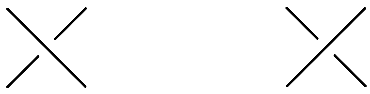
For a crossing $\mathfrak{c}_{i}=(x_{j},x_{k},x_{\ell})$ as given in Figure 10, denote $j,k,\ell$ by $\overline{i},\underline{i},i^{\prime}$, respectively.

Figure 10: Left: a positive crossing. Right: a negative crossing.

When $\mathfrak{c}_{i}$ is positive, the corresponding relator is $r_{i}=x_{j}x_{k}x_{j}^{-1}x_{\ell}^{-1}$,

$$\frac{\partial r_{i}}{\partial x_{j}}=1-x_{j}x_{k}x_{j}^{-1},\qquad\frac{\partial r_{i}}{\partial x_{k}}=x_{j},\qquad\frac{\partial r_{i}}{\partial x_{\ell}}=-x_{j}x_{k}x_{j}^{-1}x_{\ell}^{-1},$$

so

$$\Phi\big(\frac{\partial r_{i}}{\partial x_{j}}\big)=1-t_{k},\qquad\Phi\big(\frac{\partial r_{i}}{\partial x_{k}}\big)=t_{j},\qquad\Phi\big(\frac{\partial r_{i}}{\partial x_{\ell}}\big)=-1;$$

when $\mathfrak{c}_{i}$ is negative, the corresponding relator is $r_{i}=x_{j}^{-1}x_{k}x_{j}x_{\ell}^{-1}$,

$$\frac{\partial r_{i}}{\partial x_{j}}=-x_{j}^{-1}+x_{j}^{-1}x_{k},\qquad\frac{\partial r_{i}}{\partial x_{k}}=x_{j}^{-1},\qquad\frac{\partial r_{i}}{\partial x_{\ell}}=-x_{j}^{-1}x_{k}x_{j}x_{\ell}^{-1},$$

so

$$\Phi\big(\frac{\partial r_{i}}{\partial x_{j}}\big)=t_{j}^{-1}(t_{k}-1),\qquad\Phi\big(\frac{\partial r_{i}}{\partial x_{k}}\big)=t_{j}^{-1},\qquad\Phi\big(\frac{\partial r_{i}}{\partial x_{\ell}}\big)=-1.$$

In either case (remembering that $t_{\ell}=t_{k}$),

$$\Phi\Big(\frac{\partial r_{i}}{\partial x_{j}},\frac{\partial r_{i}}{\partial x_{k}},\frac{\partial r_{i}}{\partial x_{\ell}}\Big)\left(\begin{array}[]{ccc}1-t_{j}&&\\ &1-t_{k}&\\ &&1-t_{\ell}\end{array}\right)=(1-t_{k})(1-t_{j}^{\epsilon},t_{j}^{\epsilon},-1),$$ (6)

where $\epsilon=1$ (resp. $\epsilon=-1$) if $\mathfrak{c}_{i}$ is positive (resp. negative).

Thus, as shown in the beginning of [4, Section 3], $MD=D^{\prime}Q$, where

• $D$ is the $n\times n$ diagonal matrix whose $j$-th diagonal entry is $1-t_{j}$;

• $D^{\prime}$ is the $n\times n$ diagonal matrix whose $i$-th diagonal entry is $1-t_{i^{\prime}}$;

• $Q_{i,\overline{i}}=1-t_{\overline{i}}^{\epsilon}$, $Q_{i,\underline{i}}=t_{\overline{i}}^{\epsilon}$, $t_{i,i^{\prime}}=-1$, where $\epsilon=1$ (resp. $\epsilon=-1$) if $\mathfrak{c}_{i}$ is positive (resp. negative), and $Q_{i,j}=0$ for $j\notin\{\overline{i},\underline{i},i^{\prime}\}$.

For any $i,j$, let $M_{\neg i}^{\neg j}$ denote the matrix obtained from $M$ by deleting the $i$-th row and the $j$-th column. Then $M_{\neg i}^{\neg j}D_{\neg j}^{\neg j}=(D^{\prime})^{\neg i}_{\neg i}Q_{\neg i}^{\neg j}$, so

$$\Delta_{L}\doteq\frac{\det\big(M_{\neg i}^{\neg j}\big)}{1-t_{j}}\doteq\frac{\det\big(Q_{\neg i}^{\neg j}\big)}{1-t_{i^{\prime}}}\doteq\frac{\det\big(Q_{\neg i}^{\neg j}\big)}{1-t_{\underline{i}}},$$ (7)

the last equality following from that $x_{i^{\prime}}$ is conjugate to $x_{\underline{i}}$.

We shall do elementary transformations to convert $Q$ into another matrix which is highly simplified. To speak conveniently, introduce for each direct arc $z$ a formal variable $\xi_{z}$. Each row of $Q$ corresponds to an equation $\sum_{j=1}^{m}Q_{i,j}\xi_{x_{j}}=0,$ and doing row-transformations is equivalent to re-writing equations of such kind. Note that $\xi_{z}$ depends only on the underlying arc of $z$, so $\xi_{z^{\prime}}$ also makes sense for an un-directed arc $z^{\prime}$.

Claim 4.2.

For each $S\in\mathcal{T}_{\rm ar}^{\rm or}$ that is a subtangle of $T$, let $Q_{S}$ denote the matrix constructed similarly as $Q$. Let $\xi^{\rm nw}=\xi_{S^{\rm nw}}$, etc.

1. There exist an invertible matrix $U_{v}$ such that $U_{v}^{-1}Q_{S}\vec{\xi}=0$ is equivalent to $\xi_{x}=(1-b_{x})\xi^{\rm nw}+b_{x}\xi^{\rm ne}$ for all $x$.

2. There exist an invertible matrix $U_{h}$ such that $U_{h}^{-1}Q_{S}\vec{\xi}=0$ is equivalent to $\xi_{x}=(1-c_{x})\xi^{\rm nw}+c_{x}\xi^{\rm sw}$ for all $x$.

In particular, with $b^{\rm nw}=b_{S^{\rm nw}}$, $c^{\rm nw}=c_{S^{\rm nw}}$, etc.,

$$\left(\begin{array}[]{cc}\xi^{\rm sw}\\ \xi^{\rm se}\end{array}\right) =F_{v}(S)\left(\begin{array}[]{cc}\xi^{\rm nw}\\ \xi^{\rm ne}\end{array}\right),\qquad F_{v}(S)=\left(\begin{array}[]{cc}1-b^{\rm sw}&b^{\rm sw}\\ 1-b^{\rm se}&b^{\rm se}\end{array}\right),$$

$$\left(\begin{array}[]{cc}\xi^{\rm ne}\\ \xi^{\rm se}\end{array}\right) =F_{h}(S)\left(\begin{array}[]{cc}\xi^{\rm nw}\\ \xi^{\rm sw}\end{array}\right),\qquad F_{h}(S)=\left(\begin{array}[]{cc}1-c^{\rm ne}&c^{\rm ne}\\ 1-c^{\rm se}&c^{\rm se}\end{array}\right).$$

Let $z_{v}(S)=\det(U_{v})$, $z_{h}(S)=\det(U_{h})$.

Proof.

First we point out that (i) is equivalent to (ii). Suppose the rows in $U_{v}^{-1}Q_{S}$ corresponding to $(\xi^{\rm sw},\xi^{\rm se})^{\rm tr}=F_{v}(S)(\xi^{\rm nw},\xi^{\rm ne})^{\rm tr}$ are the first and second rows in the following table:

$\xi^{\rm nw}$	$\xi^{\rm ne}$	$\xi^{\rm sw}$	$\xi^{\rm se}$
$1-b^{\rm sw}$	$b^{\rm sw}$	$-1$	0
$1-b^{\rm se}$	$b^{\rm se}$	0	$-1$
$1-1/b^{\rm sw}$	$-1$	$1/b^{\rm sw}$	0
$1-b^{\rm se}/b^{\rm sw}$	0	$b^{\rm se}/b^{\rm sw}$	$-1$

Then we can express $\xi^{\rm ne},\xi^{\rm se}$ as linear combinations of $\xi^{\rm nw},\xi^{\rm sw}$, corresponding to the third and fourth rows. So $c^{\rm ne}=1/b^{\rm sw}$, $c^{\rm se}=b^{\rm se}/b^{\rm sw}$.

Furthermore, note that the third row results from multiplying the first row by $-1/b^{\rm sw}$, and the fourth one can be obtained by subtracting $b^{\rm se}/b^{\rm sw}$ times the first row from the second row. Consequently,

$$z_{h}(S)=-b^{\rm sw}z_{v}(S).$$ (8)

The situation is similar for turning from (ii) to (i).

The claim is clearly true for $[\pm 1]$. Suppose $S=S_{1}\ast S_{2}$ and the claim holds for $S_{1},S_{2}$, then $\xi^{\rm nw}=\xi_{1}^{\rm nw}$, $\xi^{\rm ne}=\xi_{1}^{\rm ne}$, $\xi^{\rm sw}=\xi_{2}^{\rm sw}$, $\xi^{\rm se}=\xi_{2}^{\rm se}$. And it is clear that $F_{v}(S)=F_{v}(S_{2})F_{v}(S_{1})$.

$\xi_{1}^{\rm nw}$	$\xi_{1}^{\rm ne}$	$\xi_{1}^{\rm sw}=\xi_{2}^{\rm nw}$	$\xi_{1}^{\rm se}=\xi_{2}^{\rm ne}$	$\xi_{2}^{\rm sw}$	$\xi_{2}^{\rm se}$
$1-b_{1}^{\rm sw}$	$b_{1}^{\rm sw}$	$-1$
$1-b_{1}^{\rm se}$	$b_{1}^{\rm se}$		$-1$
		$1-b_{2}^{\rm sw}$	$b_{2}^{\rm sw}$	$-1$
		$1-b_{2}^{\rm se}$	$b_{2}^{\rm se}$		$-1$
$1-b_{1}^{\rm sw}$	$b_{1}^{\rm sw}$	$-1$
$1-b_{1}^{\rm se}$	$b_{1}^{\rm se}$		$-1$
$1-b_{2}^{\rm sw}$	$b_{2}^{\rm sw}$			$-1$
$1-b_{2}^{\rm se}$	$b_{2}^{\rm se}$				$-1$

From the table we can see that substituting $\xi_{2}^{\rm nw}$, $\xi_{2}^{\rm ne}$ by linear combinations of $\xi_{1}^{\rm nw}$, $\xi_{1}^{\rm ne}$ corresponds to the left multiplication by a matrix of determinant $1$. So $z_{v}(S)=z_{v}(S_{1})z_{v}(S_{2})$.

The situation is similar when $S=S_{1}+S_{2}$. ∎

Ultimately, $Q_{T}$ is transformed into

$$U^{-1}Q_{T}\Omega=\left(\begin{array}[]{cccccc}1-b_{1}&b_{1}&-1&&&\\ \vdots&\vdots&&\ddots&&\\ 1-b^{\rm sw}&b^{\rm sw}&&&-1&\\ 1-b^{\rm se}&b^{\rm se}&&&&-1\end{array}\right),$$

where $U$ is invertible with $\det(U)=z_{v}(T)$, and $\Omega$ is a permutation matrix for arranging the columns so that the last two ones correspond to $T^{\rm sw}$, $T^{\rm se}$.

Note that $U^{-1}Q$ can be obtained from $U^{-1}Q_{T}$ by deleting the last two columns, and modifying the last two rows according to $\xi^{\rm nw}=\xi^{\rm sw}$ (just because that in $L$ they are the same) and $\xi^{\rm ne}=\xi^{\rm se}$. Hence in block form,

$$U^{-1}Q=\left(\begin{array}[]{ccc}\star&\star&I_{n-2}\\ -b^{\rm sw}&b^{\rm sw}&0\\ 1-b^{\rm se}&b^{\rm se}-1&0\end{array}\right),$$

where each $\star$ stands for a column that is irrelevant. Deleting the last row (corresponding to the crossing for which $T^{\rm ne}$ is one of the lower arcs) and the first column, we obtain (for certain $i,j$)

$$\det(Q^{\neg h}_{\neg i})\doteq\det(U)\cdot b^{\rm sw}=z_{v}(T)b^{\rm sw}\stackrel{{\scriptstyle(\ref{eq:z-vs-b})}}{{=}}-z_{h}(T).$$ (9)

Furthermore, there is a “hidden” relation which will play a key role.

Suppose $S\in\mathcal{T}_{\rm ar}^{\rm or}$ which is a subtangle of $T$; suppose $S$ has $\ell$ crossings and $\ell+2$ arcs. It follows from $x^{\rm nw}x^{\rm ne}x^{\rm se}x^{\rm sw}=1$ that $t_{\rm nw}t_{\rm ne}t_{\rm se}t_{\rm sw}=1$, and

$$0 =(t_{\rm nw}-1)\xi^{\rm nw}+(t_{\rm ne}-1)t_{\rm nw}\xi^{\rm ne}+t_{\rm nw}t_{\rm ne}(t_{\rm se}-1)\xi^{\rm se}+t_{\rm sw}^{-1}(t_{\rm sw}-1)\xi^{\rm sw}$$

$$=(t_{\rm nw}-1)\xi^{\rm nw}+(t_{\rm ne}-1)t_{\rm nw}\xi^{\rm ne}+t_{\rm sw}^{-1}t_{\rm se}^{-1}(t_{\rm se}-1)(((1-b^{\rm se})\xi^{\rm nw}+b^{\rm se}\xi^{\rm ne})$$

$$\ \ \ \ +(1-t_{\rm sw}^{-1})((1-b^{\rm sw})\xi^{\rm nw}+b^{\rm sw}\xi^{\rm ne})$$

$$=\big(t_{\rm nw}-1+t_{\rm sw}^{-1}(1-t_{\rm se}^{-1})(1-b^{\rm se})+(1-t_{\rm sw}^{-1})(1-b^{\rm sw})\big)\xi^{\rm nw}$$

$$\ \ \ \ +\big((t_{\rm ne}-1)t_{\rm nw}+t_{\rm sw}^{-1}(1-t_{\rm se}^{-1})b^{\rm se}+(1-t_{\rm sw}^{-1})b^{\rm sw}\big)\xi^{\rm ne}.$$

Note that $\dim\{\mathbf{v}\in\mathbb{C}^{\ell+2}\colon Q_{S}\mathbf{v}=0\}\geq 2$, as the rank of $Q_{S}$ is $\leq\ell$, so

$$t_{\rm nw}-1+t_{\rm sw}^{-1}(1-t_{\rm se}^{-1})(1-b^{\rm se})+(1-t_{\rm sw}^{-1})(1-b^{\rm sw})=0,$$

$$(t_{\rm ne}-1)t_{\rm nw}+t_{\rm sw}^{-1}(1-t_{\rm se}^{-1})b^{\rm se}+(1-t_{\rm sw}^{-1})b^{\rm sw}=0.$$

Both equations are equivalent to

$$(1-t_{\rm se}^{-1})b^{\rm se}+(t_{\rm sw}-1)b^{\rm sw}=t_{\rm sw}t_{\rm nw}(1-t_{\rm ne})=t_{\rm se}^{-1}(t_{\rm ne}^{-1}-1).$$ (10)

We are ready to prove the rules in Theorem 2.2.

Proof of Rule 1.

Clearly,

$$\sigma(T^{\rm nw})=\sigma(T)^{\rm nw},\ \ \ \sigma(T^{\rm se})=\sigma(T)^{\rm se},\ \ \ \sigma(T^{\rm ne})=\sigma(T)^{\rm sw},\ \ \ \sigma(T^{\rm sw})=\sigma(T)^{\rm ne}.$$

For $a\in\mathcal{D}(T)$, let $a^{\prime}$ denote directed arc obtained by reflecting $a$ along the diagonal and reversing the orientation. As shown in Figure 11, there is a bijective correspondence between the crossings of $T$ and those of $\sigma(T)$, via $(a,b,c)\mapsto(a^{\prime},b^{\prime},c^{\prime})$. Thus $Q_{T}$ can be identified with $Q_{\sigma(T)}$. So $F_{h}(T)=F_{v}(\sigma(T))$.

Figure 11: The two possibilities for the action of $\sigma$ on a crossing.

∎

Proof of Rule 2.

Recall that $-z_{h}(S)/z_{v}(S)$ equals $b_{S}^{\rm sw}$, the $(1,2)$-entry of $F_{v}(S)$. Let $t_{\rm ne}=\Phi(S_{1}^{\rm ne})$, $t_{\rm se}=\Phi(S_{1}^{\rm se})$, $t_{\rm sw}=\Phi(S_{1}^{\rm sw})$.

It follows from $F_{v}(S_{1}\ast S_{2})=F_{v}(S_{2})F_{v}(S_{1})$ that

$$b^{\rm sw}_{S_{1}\ast S_{2}} =b_{S_{1}}^{\rm sw}-b_{S_{1}}^{\rm sw}b_{S_{2}}^{\rm sw}+b_{S_{1}}^{\rm se}b_{S_{2}}^{\rm sw}$$

$$=b_{S_{1}}^{\rm sw}-b_{S_{1}}^{\rm sw}b_{S_{2}}^{\rm sw}+\frac{t_{\rm se}^{-1}(t_{\rm ne}^{-1}-1)+(1-t_{\rm sw})b_{S_{1}}^{\rm sw}}{1-t_{\rm se}^{-1}}b_{S_{2}}^{\rm sw}$$

$$=b_{S_{1}}^{\rm sw}+\frac{1-t_{\rm ne}^{-1}}{1-t_{\rm se}}b_{S_{2}}^{\rm sw}+\frac{t_{\rm se}^{-1}-t_{\rm sw}}{1-t_{\rm se}^{-1}}b_{S_{1}}^{\rm sw}b_{S_{2}}^{\rm sw};$$ (11)

in the second equality, (10) is used.

The composition rule for $z_{h}(S_{1}\ast S_{2})/z_{v}(S_{1}\ast S_{2})$ follows.

The rule for $z_{v}(S_{1}+S_{2})/z_{h}(S_{1}+S_{2})$ can be deduced by Rule 1. ∎

Proof of Rule 3.

Up to $\doteq$, each row of $Q$ can be multiplied by $\pm t_{j}^{\pm 1}$ whenever necessary, so we can just set $z_{h}([\pm 1])=1$.

From (6) it is easy to see $z_{v}([1])=-t_{\rm se}$, and $z_{v}([-1])=-1$.

For $[2]=T_{1}+T_{2}$, with $T_{1}=T_{2}=[1]$, let $t_{1}=t_{\rm ne}$, $t_{2}=t_{\rm se}$. We have $z_{v}(T_{1})=-t_{1}$, $z_{v}(T_{2})=-t_{2}$, hence

$$z_{v}([2])=z_{v}(T_{1})+\frac{1-t_{2}^{-1}}{1-t_{1}^{-1}}z_{v}(T_{2})+\frac{t_{2}^{-1}-t_{1}}{1-t_{1}}z_{v}(T_{1})z_{v}(T_{2})=t_{1}(t_{2}-1).$$

For $k\geq 0$, noting $t_{\rm ne}=t_{1}$, $t_{\rm se}=t_{2}$, we see

$$z_{v}([2k]) =z_{v}([2])+z_{v}([2k-2])+\frac{t_{1}^{-1}-t_{2}}{1-t_{2}}z_{v}([2])z_{v}([2k-2])$$

$$=t_{1}(t_{2}-1)+t_{1}t_{2}z_{v}([2k-2]),$$

so as to recursively deduce

$$z_{v}([2k])=\frac{(t_{1}^{k}t_{2}^{k}-1)(t_{2}-1)}{t_{2}-t_{1}^{-1}}=t_{1}(t_{2}-1)[k]_{t_{1}t_{2}}.$$ (12)

For any $\ell\geq 0$, with $t_{1}=t_{\rm se}$, $t_{2}=t_{\rm ne}$,

$$z_{v}([2\ell+1]) =z_{v}([2\ell])+z_{v}([1])+\frac{t_{1}^{-1}-t_{2}}{1-t_{2}}z_{v}([2\ell])z_{v}([1])$$

$$=t_{1}(t_{2}-1)[\ell]_{t_{1}t_{2}}-t_{1}^{\ell+1}t_{2}^{\ell}=(1-t_{1})[\ell+1]_{t_{1}t_{2}}-1.$$ (13)

For $[-2]=T_{1}+T_{2}$, with $T_{1}=T_{2}=[-1]$, we have $z_{v}(T_{1})=z_{v}(T_{2})=-1$, hence with $t_{1}=t_{\rm ne}$, $t_{2}=t_{\rm se}$,

$$z_{v}([-2])=z_{v}(T_{1})+\frac{1-t_{2}^{-1}}{1-t_{1}^{-1}}z_{v}(T_{2})+\frac{t_{2}^{-1}-t_{1}}{1-t_{1}}z_{v}(T_{1})z_{v}(T_{2})=t_{2}^{-1}-1.$$

For $k>0$, similarly as $z_{v}([2k])$, we have

$$z_{v}([-2k])=z_{v}([-2])+t_{1}^{-1}t_{2}^{-1}z_{v}([-(2k-2)]),$$

so as to recursively deduce

$$z_{v}([-2k])=\frac{(t_{1}^{-k}t_{2}^{-k}-1)(t_{2}-1)}{t_{2}-t_{1}^{-1}}=t_{1}(t_{2}-1)[-k]_{t_{1}t_{2}}.$$

This can be incorporated with (12).

For any $\ell\geq 0$, with $t_{1}=t_{\rm se}$, $t_{2}=t_{\rm ne}$,

$$z_{v}([-2\ell-1]) =z_{v}([-2\ell])+z_{v}([-1])+\frac{t_{1}^{-1}-t_{2}}{1-t_{2}}z_{v}([-2\ell])z_{v}([-1])$$

$$=\frac{(t_{1}^{-\ell}t_{2}^{-\ell}-1)(t_{2}-1)}{t_{2}-t_{1}^{-1}}-t_{1}^{-\ell}t_{2}^{-\ell}=(1-t_{1})[-\ell]_{t_{1}t_{2}}-1,$$

which together with (13) verify the formula for $z_{v}([2h-1])$, $h\in\mathbb{Z}$. ∎

When Rule 1–3 have been established, the proof of Theorem 2.2 is finished by combining (7) and (9).

Haimiao Chen (orcid: 0000-0001-8194-1264) chenhm@math.pku.edu.cn
Department of Mathematics, Beijing Technology and Business University,
Liangxiang Higher Education Park, Fangshan District, Beijing, China.

References

• [1] Y. Bae, I.S. Lee, On Alexander polynomials of pretzel links, Kyungpook Math. J. 60 (2020), 239–253.
• [2] Y. Belousov, Explicit formulas for the Alexander polynomial of pretzel knots, arXiv: 2502.10370.
• [3] F. Bonahon and L. Siebenmann, New geometric splittings of classical knots and the classification and symmetries of arborescent knots, unpublished manuscript (2016).
• [4] H.-M. Chen, Computing twisted Alexander polynomials for Montesinos links, Indian J. Pure Appl. Math. 52 (2021), 584–598.
• [5] H.-M. Chen, The ${\rm SL}(2,\mathbb{C})$-character variety of a Montesinos knot, Stud. Sci. Math. Hung. 59 (2022), no. 1, 75–91.
• [6] R.I. Hartley, On two-bridged knot polynomials, J. Austral. Math. Soc. (Ser. A) 28 (1979), no. 2, 241–249.
• [7] E. Hironaka, The Lehmer polynomial and pretzel links, Canad. Math. Bull. 44 (2001), no. 4, 440–451.
• [8] M. Hirasawa, K. Murasugi, Stable Alexander polynomials of arborescent links, J. Knot Theory Ramifications 28 (2019), no. 13, 1940017, 21 pp.
• [9] J. Hoste, A note on Alexander polynomials of 2-bridge links, J. Knot Theory Ramifications 29 (2020), no. 8, 1971003, 7 pp.
• [10] T. Kanenobu, Alexander polynomials of two-bridge links, J. Austral. Math. Soc. (Series A) 36 (1984), 59–68.
• [11] D. Kim, J. Lee, Some invariants of pretzel links, Bull. Austral. Math. Soc. 75 (2007), 253–271.
• [12] J.P. Levine, Links with Alexander polynomial zero, Indiana Univ. Math. J. 36 (1987), no. 1, 91–108.
• [13] W.B.R. Lickorish, An introduction to knot theory, Graduate Texts in Mathematics, vol. 175, Springer New York, 1997.
• [14] Y. Nakagawa, On the Alexander polynomials of the pretzel links $L(p_{1},\ldots,p_{n})$, Kobe J. Math. 3 (1986), 167–177.