A Gradient Sampling Algorithm for Noisy Nonsmooth Optimization

An algorithm is proposed, analyzed, and tested for minimizing locally Lipschitz objective functions that may be nonconvex and/or nonsmooth. The algorithm, which is built upon the gradient-sampling methodology, is designed specifically for cases when objective function and generalized gradient values might be subject to bounded uncontrollable errors. Similarly to state-of-the-art guarantees for noisy smooth optimization of this kind, it is proved for the algorithm that, with probability one, either the sequence of objective function values will decrease without bound or the algorithm will generate an iterate at which a measure of stationarity is below a threshold that depends proportionally on the error bounds for the objective function and generalized gradient values. The results of numerical experiments are presented, which show that the algorithm can indeed perform approximate optimization robustly despite errors in objective and generalized gradient values.

1 Introduction

Modern applications in a diverse set of areas, including machine learning and operations research, require solving optimization problems where the objective functions are merely presumed to be locally Lipschitz, meaning that they may be nonsmooth and/or nonconvex. In such settings, classical derivative-based algorithms such as gradient descent can fail easily since they rely on the objective function being differentiable and the gradient function being continuous throughout the domain. General locally Lipschitz optimization, on the other hand, requires specialized algorithms. One of the most successful frameworks for solving such challenging problems is the gradient sampling (GS) methodology. Originally introduced and analyzed in foundational work by Burke, Lewis, and Overton [6], and later refined by Kiwiel [29], this methodology involves evaluating gradients at points that are sampled randomly in a neighborhood around each iterate to construct a search direction that reliably approximates a direction of descent. Subsequent research has significantly expanded this framework to include adaptive sampling strategies, quasi-Newton acceleration, and sequential quadratic programming methods for solving constrained problems; see, e.g., the articles [8, 9, 10, 11, 12, 13], as well as the survey paper [5].

Despite these efforts in algorithm design and analysis, all previously proposed GS methods share the common assumption that exact objective function and generalized gradient values are available. However, for many modern settings, the algorithm only has access to inexact values. (Throughout the paper, we use inexact values, noisy values, values subject to error, and related such terms interchangeably when discussing situations in which exact function and/or derivative values are unavailable to an algorithm.) Such inexactness is often unavoidable, arising from numerical approximation, simulation-based modeling, or stochastic estimation procedures. In the smooth optimization regime, the challenges posed by such inexactness are well documented; researchers have developed various algorithms for solving both unconstrained and constrained problems with rigorous convergence and complexity guarantees that account for different types of noise models; see §1.2. In the context of a GS method for the more general locally Lipschitz setting, however, noisy optimization has not been fully explored. (See §1.2 for more discussion of the related literature on different types of noise models and inexact generalized-gradient-based methods for solving nonsmooth optimization problems.) It is not surprising that, in this more general setting, errors are particularly disruptive as they corrupt the sampled gradient information, which leads to unreliability in the search direction computation and compromises the algorithm’s convergence guarantees. This gap in the literature motivates the design of a GS framework that is designed specifically to handle errors in the objective function and generalized gradient evaluations while maintaining rigorous convergence guarantees that are consistent with the noiseless setting.

1.1 Contributions

The primary contributions of this work are the design and analysis of a GS-based algorithm for solving nonconvex and nonsmooth optimization problems that remains robust in the presence of errors in both the objective function and generalized gradient values, particularly when the errors in these quantities are only assumed to be bounded, and so may be biased, nonvanishing, and uncontrollable by the algorithm. Unlike previous GS methods that assume exact evaluations—and consistent with previously proposed gradient-based methods for noisy smooth optimization—our approach incorporates a threshold within the backtracking line search to prevent the failure of the search in the presence of noise. We provide a detailed theoretical analysis proving that, with probability one, the algorithm either generates objective function values that decrease without bound or it generates an iterate satisfying a stationary condition whose accuracy is tied directly to the magnitudes of the evaluation errors. Overall, our proposed method extends classical gradient sampling theory by accounting for noise that is unavoidable in numerous settings of interest. To the best of our knowledge, the proposed method is the first gradient-sampling method that explicitly incorporates bounded evaluation errors in both objective and generalized gradient information while preserving convergence guarantees.

1.2 Literature Review

In this subsection, we recall some articles in the literature that pertain to generalized-gradient-based methods for solving nonsmooth optimization problems when objective function and/or generalized gradient values may be subject to inexactness/noise/errors. We close this subsection by providing some arguments about why it is particularly attractive to consider the extension of the gradient-sampling methodology to settings where values are subject to noise.

The literature on noisy optimization can be classified in a variety of ways. One major distinction is whether the noise in the function and/or derivative information is deterministic or stochastic. Roughly speaking, deterministic noise refers to situations in which two calls to an evaluation oracle with the same optimization-variable input always produce the same value, whereas stochastic noise refers to situations in which any call to an oracle—even with the same optimization-variable input—might produce a different value. The former type of noise may arise, for example, from computational noise [1, 35] generated through a numerical simulation, say for solving a discretized partial differential equation. On the other hand, the latter type of noise may arise, e.g., in stochastic-gradient-type methods for solving machine learning problems [4].

There is a long history of work on stochastic/noisy subgradient-type methods for solving both convex and nonconvex unconstrained nonsmooth minimization problems; see, e.g., [2, 3, 16, 20, 30, 32, 33, 34, 38, 39, 40]. See also [18] for a more general setting of stochastic model-based optimization with complexity guarantees. The method in [17], which builds off of the work in [42], can be viewed as being related to a GS approach like the one that we propose, although it is quite distinct in spirit; the method is normalized/randomized gradient method with complexity guarantees. Let us emphasize that, while some of these cited methods have theoretical guarantees for certain nonconvex problems, the guarantees require somewhat restrictive assumptions, such as weak convexity. By contrast, GS methods are applicable to a larger class of locally Lipschitz minimization problems.

More closely related to our general setting is the literature on proximal-bundle methods, many of which, like GS methods, have theoretical guarantees for locally Lipschitz minimization under generally loose assumptions. In terms of proximal-bundle methods that assume that only inexact information is available either in the objective function and/or generalized gradient values, we refer the reader to [19, 24, 25, 26, 28, 31, 41]. Among these, let us highlight [24], which proposes and analyzes a proximal-bundle method for solving nonconvex and nonsmooth minimization problems when errors in the objective and generalized-gradient values may be subject to nonvanishing noise, as we presume in our context.

We emphasize that there are particular benefits to extending the gradient sampling methodology to noisy settings. For example, in general, GS methods are arguably much simpler to implement than proximal-bundle methods, especially when it comes to solving nonconvex problems. Compared to such proximal-bundle methods, GS methods involve fewer parameters that require careful tuning in order to obtain good performance in practice. (For example, proximal-bundle methods for solving nonconvex problems require the use of techniques known as downshifting or tilting, which introduce parameters that need to be tuned for good performance.) This advantage of the GS methodology is even more pronounced in noisy settings, where, not surprisingly, even more tunable parameters need to be introduced in order to ensure theoretical convergence guarantees. We contend that this advantage can be seen clearly for our proposed algorithm. In particular, despite having to deal with nonsmoothness, nonconvexity, and errors in objective function and generalized-gradient values, our algorithm involves relatively few parameters, and even though our theoretical guarantees require that the parameters are chosen carefully within certain bounds, our numerical experiments show that the behavior of our algorithm is reliable in practice, even when the parameter choices are not made precisely.

1.3 Notation

We use $\mathbb{N}:=\{1,2,\dots\}$ to denote the set of positive integers. We use $\mathbb{R}$ to denote the set of real numbers, $\mathbb{R}_{\geq r}$ (respectively, $\mathbb{R}_{>r}$) to denote the set of real numbers greater than or equal to (respectively, greater than) $r\in\mathbb{R}$, $\mathbb{R}^{n}$ to denote the set of real $n$-vectors, and $\mathbb{R}^{m\times n}$ to denote the set of real $m$-by-$n$ matrices.

Given a nonempty set ${\cal X}\subseteq\mathbb{R}^{n}$, we denote the distance function from points in the domain $\mathbb{R}^{n}$ to the set ${\cal X}$ by $\operatorname{dist}_{\cal X}:\mathbb{R}^{n}\to\mathbb{R}$, which is defined by

$$\operatorname{dist}_{{\cal X}}(v)=\inf_{x\in{\cal X}}\|x-v\|_{2}\ \ \text{for all}\ \ v\in\mathbb{R}^{n}.$$

We also refer to the diameter of such a set ${\cal X}$, which is defined as

$$\operatorname{diam}({\cal X})=\sup_{(x,\mkern 1.5mu\overline{\mkern-1.5mux})\in{\cal X}\times{\cal X}}\|x-\mkern 1.5mu\overline{\mkern-1.5mux}\|_{2}.$$

Given a nonnegative real-number radius $\epsilon\in\mathbb{R}_{\geq 0}$ and point $x\in\mathbb{R}^{n}$, we denote the closed Euclidean (i.e., $\ell_{2}$-norm) ball in $\mathbb{R}^{n}$ centered at $x$ with radius $\epsilon$ as

$$\mathbb{B}_{\leq\epsilon}^{n}(x):=\{\mkern 1.5mu\overline{\mkern-1.5mux}\in\mathbb{R}^{n}:\|\mkern 1.5mu\overline{\mkern-1.5mux}-x\|_{2}\leq\epsilon\}.$$

Given a function $\tilde{f}:\mathbb{R}^{n}\to\mathbb{R}$ and a scalar $r\in\mathbb{R}$, we denote the $r$-sublevel set of $\tilde{f}$ as

$${\cal L}_{r}(\tilde{f}):=\{x\in\mathbb{R}^{n}:\tilde{f}(x)\leq r\}.$$

Suppose that a function $f:\mathbb{R}^{n}\to\mathbb{R}$ is locally Lipschitz in the sense that, at each point $x\in\mathbb{R}^{n}$, there exist $\epsilon_{f,x}\in\mathbb{R}_{>0}$ and $L_{f,x}\in\mathbb{R}_{>0}$ such that

$$|f(\mkern 1.5mu\overline{\mkern-1.5mux})-f(\hat{x})|\leq L_{f,x}\|\mkern 1.5mu\overline{\mkern-1.5mux}-\hat{x}\|_{2}\ \ \text{for all}\ \ (\mkern 1.5mu\overline{\mkern-1.5mux},\hat{x})\in\mathbb{B}_{\leq\epsilon_{f,{\cal X}}}^{n}(x)\times\mathbb{B}_{\leq\epsilon_{f,{\cal X}}}^{n}(x).$$ (1)

By Rademacher’s theorem [21, 36], this implies that $f$ is continuous over $\mathbb{R}^{n}$ and differentiable almost everywhere in $\mathbb{R}^{n}$, i.e., the set of points in $\mathbb{R}^{n}$ at which it is not differentiable has a Lebesgue measure of zero [7, 14]. Following [7], we denote the Clarke generalized directional derivative function for $f$ as $f^{\circ}:\mathbb{R}^{n}\times\mathbb{R}^{n}\to\mathbb{R}$ with

$$f^{\circ}(x,d)=\limsup_{\begin{subarray}{c}\mkern 1.5mu\overline{\mkern-1.5mux}\to x\\ \alpha\searrow 0\end{subarray}}\frac{f(\mkern 1.5mu\overline{\mkern-1.5mux}+\alpha d)-f(\mkern 1.5mu\overline{\mkern-1.5mux})}{\alpha}\ \ \text{for all}\ \ (x,d)\in\mathbb{R}^{n}\times\mathbb{R}^{n}.$$

Subsequently, we denote the Clarke generalized gradient mapping for $f$—a set-valued mapping—by $\eth f:\mathbb{R}^{n}\rightrightarrows\mathbb{R}^{n}$, which is defined for all $x\in\mathbb{R}^{n}$ by

$$\eth f(x):= \ \{g\in\mathbb{R}^{n}:f^{\circ}(x,d)\geq g^{T}d\ \text{for all}\ d\in\mathbb{R}^{n}\}$$

$$= \ \operatorname{conv}(\{g\in\mathbb{R}^{n}:\{\nabla f(x_{k})\}\to g\ \text{for some}\ \{x_{k}\}\to x\ \text{with}\ \{x_{k}\}\subset{\cal D}_{\nabla f}\}).$$

Here, we use ${\cal D}_{\nabla f}\subseteq\mathbb{R}^{n}$ to denote the full-measure set in $\mathbb{R}^{n}$ over which $f$ is differentiable. For the equivalence indicated by the latter equation above, see, e.g., [7, 14, 37].

1.4 Organization

In §2, we state our optimization problem of interest, the assumptions that we make about the errors (i.e., noise) that may be present in the objective function and generalized gradient values, and our proposed algorithm. In §3, we present our theoretical convergence analysis of our proposed algorithm, which shows that, unless the sequence of objective values decreases without bound, the algorithm eventually generates an iterate at which a measure of stationary with respect to the optimization problem is below a threshold that depends on the bounds on the errors in the objective function and generalized gradient values. We present the results of numerical experiments in §4 and concluding remarks in §5.

2 Problem and Algorithm Statements

Our proposed algorithm is designed to solve (approximately) the problem of minimizing an objective $f:\mathbb{R}^{n}\to\mathbb{R}$, as in

$$\min_{x\in\mathbb{R}^{n}}\ f(x),$$ (2)

where $f$, along with a corresponding approximation function $\tilde{f}$ that is employed by the algorithm, at least satisfy the following assumption (recall (1)).

Assumption 2.1.

The objective function $f:\mathbb{R}^{n}\to\mathbb{R}$ is locally Lipschitz. In addition, there exists a positive real number $\epsilon_{f}\in\mathbb{R}_{>0}$ and an approximation function $\tilde{f}:\mathbb{R}^{n}\to\mathbb{R}$ such that, at any $x\in\mathbb{R}^{n}$, the algorithm can obtain $\tilde{f}(x)$ such that

$$|\tilde{f}(x)-f(x)|\leq\epsilon_{f}.$$ (3)

Moreover, given the starting point $x_{1}\in\mathbb{R}^{n}$ employed by the algorithm, there exists an open set ${\cal X}\subseteq\mathbb{R}^{n}$ containing the sublevel set ${\cal L}_{\tilde{f}(x_{1})}(\tilde{f})$ over which $f$ is Lipschitz continuous and for which the algorithm has a Lipschitz constant, i.e., the algorithm has access to a Lipschitz constant $L_{f,{\cal X}}\in\mathbb{R}_{>0}$ for $f$ over ${\cal X}$ such that

$$|f(\mkern 1.5mu\overline{\mkern-1.5mux})-f(\hat{x})|\leq L_{f,{\cal X}}\|\mkern 1.5mu\overline{\mkern-1.5mux}-\hat{x}\|_{2}\ \ \text{for all}\ \ (\mkern 1.5mu\overline{\mkern-1.5mux},\hat{x})\in{\cal X}\times{\cal X}.$$

Under Assumption 2.1, the true objective function $f$ may be nonconvex and/or nonsmooth over ${\cal X}$. The existence of $\epsilon_{f}$ and $\tilde{f}$ such that (3) holds for all $x\in\mathbb{R}^{n}$ is a common assumption in the context of noisy smooth optimization; see, e.g., [1, 35]. Let us emphasize that, under Assumption 2.1, any two evaluations of the approximation function $\tilde{f}$ at the same point $x\in\mathbb{R}^{n}$ always yield the same value, namely, $\tilde{f}(x)$. The strongest part of Assumption 2.1 is the assumption that the algorithm has access to a Lipschitz constant for $f$ over an open set ${\cal X}\supset{\cal L}_{\tilde{f}(x_{1})}(\tilde{f})$. We emphasize that the Lipschitz constant required here is for the true objective function $f$ while the sublevel set over which it is defined is for the approximation function $\tilde{f}$. This is since the algorithm works with $\tilde{f}$ whereas our theoretical analysis requires knowledge of the Lipschitz constant for $f$. We do not assume that $\tilde{f}$ is Lipschitz continuous; indeed, under Assumption 2.1, it may even be discontinuous. Knowledge of such a Lipschitz constant $L_{f,{\cal X}}$ is not required, e.g., by the algorithms for noisy smooth optimization in [1, 35], and it is also not needed for gradient sampling methods when objective function and gradient values can be obtained without error. However, it is needed for the convergence guarantees for our proposed method. Fortunately, in many situations, even with noisy function evaluations, it is reasonable to assume that one has access to at least a large estimate of such a Lipschitz constant. We further justify this part of Assumption 2.1 later in this section, and discuss along with our conclusions in §5 some approaches that one can employ to compute/estimate such a Lipschitz constant in practical applications of our proposed algorithm.

As is generally the case for nonsmooth optimization, we assume that at any point $x\in\mathbb{R}^{n}$ it is intractable to compute the entire set of generalized gradients $\eth f(x)$, although it is tractable to compute (or at least approximate) an element of $\eth f(x)$. Along these lines, for our proposed algorithm, we make the following assumption about the generalized gradient approximation function that is available to the algorithm.

Assumption 2.2.

There exists a positive real number $\epsilon_{g}\in\mathbb{R}_{>0}$ and a function $\tilde{g}:\mathbb{R}^{n}\to\mathbb{R}^{n}$ such that, at any $x\in\mathbb{R}^{n}$, the algorithm can obtain $\tilde{g}(x)$ such that

$$\|\tilde{g}(x)-g\|_{2}\leq\epsilon_{g}\ \ \text{for all}\ \ g\in\eth f(x).$$ (4)

Let us emphasize that, under Assumption 2.2, two evaluations of $\tilde{g}$ at the same point $x$ always yield the same value $\tilde{g}(x)$. Moreover, let us note that for any $x\in{\cal D}_{\nabla f}$, one has that $\eth f(x)=\{\nabla f(x)\}$ [7, 14], in which case the inequality in (4) reduces simply to $\|\tilde{g}(x)-\nabla f(x)\|_{2}\leq\epsilon_{g}$, which is a typical noise bound in the context of noisy smooth optimization; see, e.g., [1, 35]. That being said, for Assumption 2.2 in the nonsmooth case to hold, the error bound $\epsilon_{g}\in\mathbb{R}_{>0}$ needs to be large enough to account for the fact that $\tilde{g}(x)$ might be computed in a manner such that it does not approximate the closest element in $\eth f(x)$ from $\tilde{g}(x)$. We highlight this challenge in noisy nonsmooth optimization with the following realistic example.

Example 2.1.

Given a continuously differentiable function $\phi:\mathbb{R}\to\mathbb{R}$, consider the composite objective function $f:\mathbb{R}\to\mathbb{R}$ defined by $f(x)=|\phi(x)|$ for all $x\in\mathbb{R}$. Suppose that, at any $x\in\mathbb{R}$, the algorithm obtains $\tilde{\phi}(x)$ and $\tilde{f}(x)$ satisfying

$$|\tilde{\phi}(x)-\phi(x)|\leq 0.02\ \ \text{and}\ \ |\tilde{f}(x)-f(x)|\leq 0.02,\ \ \text{respectively},$$ (5)

and, similarly as for the noiseless setting, it can obtain

$$\tilde{g}(x)=\begin{cases}-\phi^{\prime}(x)&\text{if $\tilde{\phi}(x)<0$}\\ 0&\text{if $\tilde{\phi}(x)=0$}\\ \phi^{\prime}(x)&\text{if $\tilde{\phi}(x)>0$.}\end{cases}$$ (6)

$($This is an idealized setting in which $\phi^{\prime}(x)$ can be computed exactly, even though $\phi(x)$ cannot.$)$ Suppose in particular that at a given $x$ one has $\phi(x)=0.01$, $f(x)=0.01$, $\phi^{\prime}(x)=1$, and $\eth f(x)=\{1\}$, yet the algorithm obtains $\tilde{\phi}(x)=-0.01$ and $\tilde{f}(x)=-0.01$ satisfying (5), and so obtains $\tilde{g}(x)=-1$ from (6). Hence, Assumption 2.2 only holds if the generalized gradient noise bound satisfies $\epsilon_{g}\geq 2$, which is relatively large compared to the function evaluation noise bounds in (5).

Example 2.1 illustrates that, more generally for Assumption 2.2 to hold, the noise bound $\epsilon_{g}$ may need to be at least as large as the largest $\text{diam}(\eth f(x))$ over all $x\in\mathbb{R}^{n}$, i.e., with the set ${\cal X}$ defined in Assumption 2.1, Assumption 2.2 essentially requires

$$\epsilon_{g}\geq\sup_{x\in{\cal X}}\operatorname{diam}(\eth f(x)).$$ (7)

This is an inherent challenge for noisy nonsmooth optimization that would be present for any algorithm that is proposed in this context. To provide the reader with an illustration related to this discussion, we present Figure 1, which shows in an example similar to Example 2.1 that with noisy evaluations the bound $\epsilon_{g}$ may need to be relatively large compared to $\epsilon_{f}$ in the context of nonsmooth optimization.

Figure 1: On the left, the absolute value function and its corresponding generalized-gradient/subgradient mapping. On the right, the same mappings subject to bounded errors. We emphasize that, typically in noisy optimization, the mapping $\tilde{g}$ does not correspond to the derivative function of $\tilde{f}$; rather, one can expect that $\tilde{g}$ approximates $g$ directly, as shown in the graphs. That being said, the graphs show that for Assumption 2.2 to hold for this case, one clearly needs $\epsilon_{g}$ greater than the lower bound stated in (7); see, e.g., $x$ slightly to the right of the origin.

Let us now state our proposed algorithm, followed by some additional discussion to justify its design and our previously stated assumptions. Each iteration of our proposed algorithm operates in the following manner. Consider arbitrary $k\in\mathbb{N}$, and let $x_{k}\in\mathbb{R}^{n}$ and $\epsilon_{k}\in\mathbb{R}_{>0}$ denote the $k$th iterate and sampling radius that have been generated by the algorithm, respectively. The iteration begins by the algorithm sampling a set of $m\geq n+1$ points $\{x_{k,1},\dots,x_{k,m}\}$ from a uniform distribution in a ball of radius $\epsilon_{k}$ that is centered at $x_{k}$. (This lower bound for $m$ is consistent with gradient-sampling methods for the noiseless setting; we discuss the role that it plays in our theoretical analysis in §3.) This set of points, along with the current iterate $x_{k}$, is used to construct the matrix of generalized-gradient approximations

$$\widetilde{G}_{k}:=\begin{bmatrix}\tilde{g}(x_{k})&\tilde{g}(x_{k,1})&\cdots&\tilde{g}(x_{k,m})\end{bmatrix}.$$ (8)

Then, as in a standard gradient-sampling method, a search direction is obtained by solving the pair of quadratic optimization problems (QPs) given by

$$\left\{\begin{aligned} \min_{(\tilde{z},\tilde{d})\in\mathbb{R}\times\mathbb{R}^{n}}&\ \tilde{z}+\tfrac{1}{2}\|\tilde{d}\|_{2}^{2}\\ \operatorname{s.\!t.}&\ \widetilde{G}_{k}^{T}\tilde{d}\leq\tilde{z}\mathds{1}\end{aligned}\right\}\ \ \text{and}\ \ \left\{\begin{aligned} \max_{\tilde{y}\in\mathbb{R}^{m+1}}&\ -\tfrac{1}{2}\|\widetilde{G}_{k}\tilde{y}\|_{2}^{2}\\ \operatorname{s.\!t.}&\ \mathds{1}^{T}\tilde{y}=1,\ \tilde{y}\geq 0\end{aligned}\right\}.$$ (9)

The final main component of an iteration of our proposed algorithm is a backtracking line search that is conducted using the approximate function values that can be obtained by the algorithm. Specifically, starting from a unit step size, the line search backtracks to attempt to obtain a step size $\alpha_{k}\in(0,1]$ such that, for some user-defined parameter $\eta\in(0,1)$ and threshold $\epsilon_{\rm ls}\in\mathbb{R}_{>0}$, the following conditions are satisfied:

$$\tilde{f}(x_{k}+\alpha_{k}\tilde{d}_{k})<\tilde{f}(x_{k})-\eta\alpha_{k}\|\tilde{d}_{k}\|_{2}^{2}+\epsilon_{\rm ls}\ \ \text{and}\ \ \tilde{f}(x_{k}+\alpha_{k}\tilde{d}_{k})\leq\tilde{f}(x_{1}).$$ (10)

(Here, the latter condition merely ensures that the iterates remain within the sublevel set ${\cal L}_{\tilde{f}(x_{1})}(\tilde{f})$, which partly justifies Assumption 2.1.) However, if the line search backtracks to a step size that is too small relative to the known Lipschitz constant for $f$ over ${\cal X}$ from Assumption 2.1, then it resets the step size to zero and proceeds to the next iteration, where a new sample set is generated. As shown in our theoretical analysis, this procedure ensures that, if $x_{k}$ is far from stationarity in a certain sense, then any positive step size results in decrease in the approximation function $\tilde{f}$.

The complete algorithm is stated as Algorithm 1. Besides the perturbation in the sufficient decrease condition in (10), there are two main differences between Algorithm 1 and a standard gradient-sampling method for the noiseless setting. We comment on these two differences in the first two bullets below, then discuss the well-posedness of the requirement for the initial sampling radius $\epsilon_{1}$ in a third bullet.

Algorithm 1 Noise-Tolerant Gradient Sampling Algorithm

1:$x_{1}\in\mathbb{R}^{n}$ and $m\in\mathbb{N}$ with $m\geq n+1$

2:$(\epsilon_{f},\epsilon_{g})\in\mathbb{R}_{>0}\times\mathbb{R}_{>0}$ satisfying Assumptions 2.1–2.2

3:$\theta\in(0,1]$, $\gamma\in(0,1)$, $\eta\in(0,\tfrac{1}{2})$, and $\epsilon_{\rm ls}\in\mathbb{R}_{>2\epsilon_{f}}$

4:$L_{f,{\cal X}}\in\mathbb{R}_{>2\epsilon_{g}}$ satisfying Assumption 2.1

5:$\nu\in\mathbb{R}_{>0}$ and $\epsilon_{1}\in\left(\max\left\{\left(\frac{6\epsilon_{\rm ls}(L_{f,{\cal X}}+\epsilon_{g})}{\eta\gamma\nu^{2}}\right)^{1/3},5\epsilon_{g}\right\},3(L_{f,{\cal X}}+\epsilon_{g})\right)$

6:for $k=1,2,3,\dots$ do

7:  sample $\{x_{k,1},\dots,x_{k,m}\}$ from a uniform distribution over $\mathbb{B}_{\leq\epsilon_{k}}^{n}(x_{k})$

8:  set $\widetilde{G}_{k}$ by (8)

9:  compute $(\tilde{z}_{k},\tilde{d}_{k},\tilde{y}_{k})$ as the primal-dual solution of (9)

10:  set $\tilde{g}_{k}\leftarrow\widetilde{G}_{k}\tilde{y}_{k}=-\tilde{d}_{k}$

11:  if $\|\tilde{g}_{k}\|_{2}\leq\max\{\nu\epsilon_{k},5\epsilon_{g}\}$ then

12:   set $\epsilon_{k+1}\leftarrow\theta\epsilon_{k}$

13:   set $\alpha_{k}\leftarrow 0$

14:  else

15:   set $\epsilon_{k+1}\leftarrow\epsilon_{k}$

16:   for $j=0,1,2,\dots$ do

17:     if $\displaystyle\gamma^{j}<\frac{\gamma\epsilon_{k}}{3(L_{f,{\cal X}}+\epsilon_{g})}$ then

18:      set $\alpha_{k}\leftarrow 0$ and break

19:     else if (10) holds with $\alpha_{k}\equiv\gamma^{j}$ then

20:      set $\alpha_{k}\leftarrow\gamma^{j}$ and break

21:     end if

22:   end for

23:  end if

24:  set $x_{k+1}\leftarrow x_{k}+\alpha_{k}\tilde{d}_{k}$

25:end for

• A standard gradient-sampling method that employs exact objective function and gradient values involves an additional set of steps to ensure that $x_{k}\in{\cal D}_{\nabla f}$ for all $k\in\mathbb{N}$. We do not include such a procedure in Algorithm 1 since, in our setting, the algorithm cannot compute accurate generalized gradient values, let alone determine whether a point is included in ${\cal D}_{\nabla f}$. (In fact, even in the noiseless setting, checking for inclusion in ${\cal D}_{\nabla f}$ may be impractical, which is why implementations of gradient-sampling methods often skip these steps in any case [6].) We are able to prove our theoretical guarantees without the algorithm having such a procedure since, due to noisy function and generalized gradient evaluations, our guarantees are naturally weaker than those that can be obtained with exact values of these quantities. This is discussed further along with our assumptions and theoretical guarantees in §3.

• The algorithm’s need for $L_{f,{\cal X}}$ as defined in Assumption 2.1 is due essentially to its stochastic nature. In the setting of noisy smooth optimization, it can be shown that if an iterate $x_{k}$ is far from stationarity in the sense that $\|\nabla f(x_{k})\|_{2}\gg 0$, then, even with a perturbed sufficient decrease condition in the line search (i.e., the addition of a constant such as $\epsilon_{\rm ls}$ to the right-hand side), a step will yield decrease in the true objective function $f$. However, in the context of Algorithm 1, it is possible for the algorithm to yield insufficient decrease due to a bad sample set, i.e., not specifically due to the noise in the objective function and generalized gradient evaluators. Algorithm 1 overcomes this issue through its knowledge of the Lipschitz constant $L_{f,{\cal X}}$, which in turn informs the algorithm of a threshold for the step size that would be obtained if the current iterate is sufficiently far from stationarity and the sample set is good in some sense. (All of these notions are characterized rigorously through our theoretical analysis in the next section.) Overall, while requiring knowledge of $L_{f,{\cal X}}$ is not ideal, we are not aware of any other GS approach that has been proposed for noisy nonconvex nonsmooth optimization with theoretical convergence guarantees, let alone one that does not require knowledge of such a Lipschitz constant. It should also be said that if in practice the algorithm only has access to a conservatively large Lipschitz constant, then the only effect in the algorithm is that the threshold in Line 17 is smaller. In such a setting, Assumption 2.1 would hold, and the only bad effect in practice is that the algorithm may perform additional approximate function evaluations during the line searches. It should also be said that, in our numerical experiments, we do not make use of such a Lipschitz constant, yet obtain good performance nonetheless.

• For a gradient-sampling method in the setting where function and gradient values are computed without errors, there is no restriction on the initial sampling radius $\epsilon_{1}$. In our setting, however, the interval for the initial sampling radius is needed for two purposes. The upper bound of the interval is needed to ensure that if the current iterate is far from stationarity and the sample set is good in a certain sense, then there is a useful lower bound for the step size that will be computed by the line search; the role that the upper bound for $\epsilon_{1}$ (and so $\{\epsilon_{k}\}$) plays can be seen in the proof of Lemma 3.3 in the following section. As for the lower bound of the interval for $\epsilon_{1}$, we include it to ensure that if the sampling radius is below a critical threshold, then it must have reduced the sampling radius at least once, which in turn means that the algorithm at least produced an iterate that is approximately stationary. The details for this can be found in upcoming Theorem 3.1. It should be noted that the interval for $\epsilon_{1}$ can always be made nonempty. In particular, $L_{f,{\cal X}}>2\epsilon_{g}$ ensures that $5\epsilon_{g}<3(L_{f,{\cal X}}+\epsilon_{g})$, and for any values of the other parameters, the stationarity factor $\nu$ can be chosen sufficiently large so that the interval is nonempty, although it should be said that this increases the right-hand side in Line 11 of the algorithm.

3 Analysis

For a gradient-sampling method in the noiseless setting, one can show that an algorithm similar to Algorithm 1 (with a few additional features) generates, with probability one, a sequence of iterates over which either the objective function values diverge to $-\infty$ or for which any limit point is stationary for $f$ [5]. Such a guarantee is not reasonable to expect in a noisy setting, since with noise in objective function and generalized-gradient evaluations, one should not expect that the algorithm would be able to generate iterates that converge all the way to stationarity for $f$. That being said, one can expect that, at any point that is far from stationarity, the algorithm will generate a search direction that leads to sufficient decrease in $\tilde{f}$, which in turn may correspond to sufficient decrease in $f$, at least when the norm of the step is large relative to the error bound $\epsilon_{f}$. Consequently, our aim in this section is to show that, from any initial point, Algorithm 1 will at least generate a sequence of iterates such that, for some $k\in\mathbb{N}$, a measure of stationary with respect to $x_{k}$ is small relative to the noise in the objective function and generalized-gradient values.

Our ultimate convergence guarantee is stated in Theorem 3.1 at the end of this section. Let us preview this guarantee before commencing our analysis. The guarantee is stated in terms of the $\epsilon$-generalized gradient mapping $\eth_{\epsilon}f:\mathbb{R}^{n}\rightrightarrows\mathbb{R}^{n}$ as introduced by Goldstein [22], which is defined for all $\epsilon\in\mathbb{R}_{>0}$ and for any $x\in\mathbb{R}^{n}$ by

$$\eth_{\epsilon}f(x):=\operatorname{cl}\left(\operatorname{conv}\left({\cal U}_{f,\epsilon}(x)\right)\right),\ \ \text{where}\ \ {\cal U}_{f,\epsilon}(x):=\bigcup_{\mkern 1.5mu\overline{\mkern-1.5mux}\in\mathbb{B}_{\leq\epsilon}^{n}(x)}\eth f(\mkern 1.5mu\overline{\mkern-1.5mux}).$$

Informally, our convergence guarantee in Theorem 3.1 shows that, under reasonable assumptions and with probability one, Algorithm 1 generates $\{x_{k}\}$ over which either

1. $\{f(x_{k})\}\to-\infty$, or

2. in some iteration $k\in\mathbb{N}$, one has that $\|g\|_{2}={\cal O}(\epsilon_{g}+\max\{\epsilon_{\rm ls}^{1/3},\epsilon_{g}\})$ for some $g\in\eth_{\epsilon_{k}}f(x_{k})$ with $\epsilon_{k}={\cal O}(\max\{\epsilon_{\rm ls}^{1/3},\epsilon_{g}\})$; i.e., there exist positive real numbers $C_{\epsilon}$ and $C_{g}$ such that, for some $k\in\mathbb{N}$, one finds $\epsilon_{k}\leq C_{\epsilon}\max\{\epsilon_{\rm ls}^{1/3},\epsilon_{g}\}$ and $\|g\|_{2}\leq C_{g}(\epsilon_{g}+\max\{\epsilon_{\rm ls}^{1/3},\epsilon_{g}\})$ for some $g\in\eth_{\epsilon_{k}}f(x_{k})$.

Such a conclusion is all that one can expect in our noisy setting. It means that, with probability one, the algorithm will reduce the sampling radius to a level that is proportional to the noise bound for the generalized gradients and the perturbation factor in the line search condition (10), which in turn only needs to be proportional to the noise bound for the objective function values. Moreover, at this sampling radius, the algorithm will almost surely reach an iteration $k\in\mathbb{N}$ at which the minimum-norm element of $\eth_{\epsilon_{k}}f(x_{k})$ will have norm that is proportional to the noise bounds. We note upfront that the $\epsilon_{\rm ls}^{1/3}$ term may be surprising, since from the setting of noisy smooth optimization one might expect this term to appear as $\epsilon_{\rm ls}^{1/2}$. That is, assuming $\epsilon_{\rm ls}$ is proportional to $\epsilon_{f}$, one might expect the final accuracy to be proportional to $\max\{\epsilon_{f}^{1/2},\epsilon_{g}\}$. We discuss the reason for this different exponent after the proof of our main theorem at the end of this section, and discuss where in our analysis it arises.

Let us now commence our analysis of Algorithm 1 to reach these conclusions. Our first lemma, a related version of which is a hallmark of GS methods (see [29, Lemma 3.1]), is adapted here for our analysis of the noisy setting.

Lemma 3.1.

Suppose that ${\cal G}\subset\mathbb{R}^{n}$ is nonempty, convex, and compact, and that $\|g\|_{2}>3\epsilon_{g}$ for all $g\in{\cal G}$. Let $\tilde{{\cal G}}$ be any nonempty, convex, and compact set such that $\operatorname{dist}_{\cal G}(\tilde{g})\leq\epsilon_{g}$ for all $\tilde{g}\in\tilde{{\cal G}}$ and $\operatorname{dist}_{\tilde{\cal G}}(g)\leq\epsilon_{g}$ for all $g\in{\cal G}$. $($Note that this guarantees that $\|\tilde{g}\|_{2}>2\epsilon_{g}$ for all $\tilde{g}\in\tilde{\cal G}$.$)$ Then, for any $\eta\in(0,\tfrac{1}{2})$, there exists $\beta\in\mathbb{R}_{>0}$ such that if $\tilde{u}\in\tilde{{\cal G}}$ satisfies $\|\tilde{u}\|_{2}\leq\operatorname{dist}_{\tilde{\cal G}}(0)+\beta$, then $\tilde{u}^{T}v>\eta\|\tilde{u}\|_{2}^{2}$ for all $v\in{\cal G}$.

Proof.

Suppose that the implication is false. That is, suppose that for some $\eta\in(0,\tfrac{1}{2})$ and all $\beta\in\mathbb{R}_{>0}$, there exists $(\tilde{u},v)\in\tilde{\cal G}\times{\cal G}$ such that $\|\tilde{u}\|_{2}\leq\operatorname{dist}_{\tilde{\cal G}}(0)+\beta$ and $\tilde{u}^{T}v\leq\eta\|\tilde{u}\|_{2}^{2}$. Consider such an $\eta\in(0,\tfrac{1}{2})$. This implies that there exist infinite sequences $\{\tilde{u}_{j}\}$ and $\{v_{j}\}$ such that for all $j\in\mathbb{N}$ one has $\tilde{u}_{j}\in\tilde{\cal G}$, $v_{j}\in{\cal G}$, $\|\tilde{u}_{j}\|_{2}\leq\operatorname{dist}_{\tilde{\cal G}}(0)+1/j$, and $\tilde{u}_{j}^{T}v_{j}\leq\eta\|\tilde{u}_{j}\|_{2}^{2}$. Since ${\cal G}$ and $\tilde{\cal G}$ are compact, the sequence $\{(\tilde{u}_{j},v_{j})\}$ has a convergent subsequence. Passing to a subsequence if necessary, one can thus conclude that there exists a pair of limit points $(\mkern 1.5mu\overline{\mkern-1.5muu},\mkern 1.5mu\overline{\mkern-1.5muv})\in\tilde{\cal G}\times{\cal G}$ such that

$$\mkern 1.5mu\overline{\mkern-1.5muu}^{T}\mkern 1.5mu\overline{\mkern-1.5muv}\leq\eta\|\mkern 1.5mu\overline{\mkern-1.5muu}\|_{2}^{2}.$$ (11)

On the other hand, by the definition of the sequence $\{\tilde{u}_{j}\}$, it follows that $\mkern 1.5mu\overline{\mkern-1.5muu}=\operatorname{Proj}_{\tilde{\cal G}}(0)$, which is nonzero under the conditions of the lemma. Furthermore, let $\hat{v}=\operatorname{Proj}_{\tilde{\cal G}}(\mkern 1.5mu\overline{\mkern-1.5muv})$. By the Projection Theorem [14, Theorem 6.5] and convexity of $\tilde{\cal G}$, one has

$$(0-\mkern 1.5mu\overline{\mkern-1.5muu})^{T}(\hat{v}-\mkern 1.5mu\overline{\mkern-1.5muu})\leq 0,\ \ \text{which means}\ \ \mkern 1.5mu\overline{\mkern-1.5muu}^{T}\hat{v}\geq\|\mkern 1.5mu\overline{\mkern-1.5muu}\|_{2}^{2}.$$

Thus, under the conditions of the lemma, one finds that

$$\mkern 1.5mu\overline{\mkern-1.5muu}^{T}\mkern 1.5mu\overline{\mkern-1.5muv} =\mkern 1.5mu\overline{\mkern-1.5muu}^{T}(\hat{v}+\mkern 1.5mu\overline{\mkern-1.5muv}-\hat{v})$$

$$\geq\mkern 1.5mu\overline{\mkern-1.5muu}^{T}\hat{v}-\|\mkern 1.5mu\overline{\mkern-1.5muu}\|_{2}\|\mkern 1.5mu\overline{\mkern-1.5muv}-\hat{v}\|_{2}$$

$$\geq\|\mkern 1.5mu\overline{\mkern-1.5muu}\|_{2}^{2}-\|\mkern 1.5mu\overline{\mkern-1.5muu}\|_{2}\epsilon_{g}$$

$$=\|\mkern 1.5mu\overline{\mkern-1.5muu}\|_{2}(\|\mkern 1.5mu\overline{\mkern-1.5muu}\|_{2}-\epsilon_{g})$$

$$\geq\tfrac{1}{2}\|\mkern 1.5mu\overline{\mkern-1.5muu}\|_{2}^{2},$$

where the last inequality follows since $\|\mkern 1.5mu\overline{\mkern-1.5muu}\|>2\epsilon_{g}$, so $\tfrac{1}{2}\|\mkern 1.5mu\overline{\mkern-1.5muu}\|>\epsilon_{g}$, which means that $\|\mkern 1.5mu\overline{\mkern-1.5muu}\|_{2}-\epsilon_{g}>\|\mkern 1.5mu\overline{\mkern-1.5muu}\|_{2}-\tfrac{1}{2}\|\mkern 1.5mu\overline{\mkern-1.5muu}\|_{2}=\tfrac{1}{2}\|\mkern 1.5mu\overline{\mkern-1.5muu}\|_{2}$. However, this contradicts (11) since $\eta<\tfrac{1}{2}$. ∎

Our subsequent analysis makes use of Lemma 3.1 where ${\cal G}$ and $\tilde{\cal G}$ are defined through noiseless and noisy quantities, respectively. In particular, values of $\eth_{\epsilon}f(x)$ will play the role of the set ${\cal G}$. On the other hand, for any $\epsilon\in\mathbb{R}_{>0}$, let us also introduce the mapping $\tilde{\cal G}_{\epsilon}(x):\mathbb{R}^{n}\rightrightarrows\mathbb{R}^{n}$ as being defined for all $x\in\mathbb{R}^{n}$ by

$$\tilde{\cal G}_{\epsilon}(x):=\operatorname{cl}(\operatorname{conv}(\{\tilde{g}(\mkern 1.5mu\overline{\mkern-1.5mux}):\mkern 1.5mu\overline{\mkern-1.5mux}\in\mathbb{B}_{\leq\epsilon}^{n}(x)\})).$$ (12)

Values of this mapping will play the role of $\tilde{\cal G}$ in our subsequent use of Lemma 3.1.

The following lemma establishes a critical relationship between these quantities.

Lemma 3.2.

For all $(x,\epsilon)\in\mathbb{R}^{n}\times\mathbb{R}_{>0}$, one has that

$$\operatorname{dist}_{\eth_{\epsilon}f(x)}(g) \leq\epsilon_{g}\ \ \text{for all}\ \ g\in\tilde{\cal G}_{\epsilon}(x)$$

$$\text{and}\ \ \operatorname{dist}_{\tilde{\cal G}_{\epsilon}(x)}(g) \leq\epsilon_{g}\ \ \text{for all}\ \ g\in\eth_{\epsilon}f(x).$$

Proof.

Consider arbitrary $(x,\epsilon)\in\mathbb{R}^{n}\times\mathbb{R}_{>0}$. Let us prove the first of the two inequalities; the other follows using a similar argument. For any pair of elements, say $\tilde{g}_{1}$ and $\tilde{g}_{2}$, from $\{\tilde{g}(\mkern 1.5mu\overline{\mkern-1.5mux}):\mkern 1.5mu\overline{\mkern-1.5mux}\in\mathbb{B}_{\leq\epsilon}^{n}(x)\}$, there are $\tilde{x}_{1}\in\mathbb{B}_{\leq\epsilon}^{n}(x)$ and $\tilde{x}_{2}\in\mathbb{B}_{\leq\epsilon}^{n}(x)$ such that $\tilde{g}_{1}=\tilde{g}(\tilde{x}_{1})$ and $\tilde{g}_{2}=\tilde{g}(\tilde{x}_{2})$. Then, from Assumption 2.2, one finds that $\|\tilde{g}_{1}-g\|_{2}\leq\epsilon_{g}$ for all $g\in\eth f(\tilde{x}_{1})$ and that $\|\tilde{g}_{2}-g\|_{2}\leq\epsilon_{g}$ for all $g\in\eth f(\tilde{x}_{2})$. Consequently,

$$\operatorname{dist}_{\operatorname{conv}({\cal U}_{f,\epsilon}(x))}(g)\leq\epsilon_{g}\ \ \text{for all}\ \ g\in\operatorname{conv}(\{\tilde{g}(\mkern 1.5mu\overline{\mkern-1.5mux}):\mkern 1.5mu\overline{\mkern-1.5mux}\in\mathbb{B}_{\leq\epsilon}^{n}(x)\}).$$

(This follows since, for any point on the line segment between $\tilde{g}_{1}$ and $\tilde{g}_{2}$, there exists a point on the line segment between one point from $\eth f(\tilde{x}_{1})$ and another point from $\eth f(\tilde{x}_{2})$—i.e., an element from $\operatorname{conv}({\cal U}_{f,\epsilon}(x))$—that is at most a distance $\epsilon_{g}$ away from the point of interest between $\tilde{g}_{1}$ and $\tilde{g}_{2}$.) All that remains is to note that taking the closure of the sets preserves the upper bound of the distance as $\epsilon_{g}$. ∎

Let us now define for any $(x,\epsilon,\mkern 1.5mu\overline{\mkern-1.5mux},\beta)\in\mathbb{R}^{n}\times\mathbb{R}_{>0}\times\mathbb{R}^{n}\times\mathbb{R}_{>0}$ the set

$$\begin{split}{\cal T}(x,\epsilon,\mkern 1.5mu\overline{\mkern-1.5mux},\beta)=\Bigg\{&S\in\prod_{i\in[m]}\mathbb{B}_{\leq\epsilon}^{n}(x):\\ &\quad\operatorname{dist}_{\operatorname{conv}(\{\tilde{g}(x)\}_{x\in S})}(0)\leq\operatorname{dist}_{\tilde{\cal G}_{\epsilon}(\mkern 1.5mu\overline{\mkern-1.5mux})}(0)+\beta\Bigg\}.\end{split}$$ (13)

(Here, we overload notation and use $\{\tilde{g}(x)\}_{x\in S}$ to indicate the set of values of $\tilde{g}$ evaluated at the elements in the tuple $S$.) Intuitively, such a set identifies the sample sets that are good enough to guarantee that the minimum-norm element of $\tilde{\cal G}_{\epsilon}(\mkern 1.5mu\overline{\mkern-1.5mux})$ is approximated well enough by the minimum-norm element of $\operatorname{conv}(\{\tilde{g}(x)\}_{x\in S})$ corresponding to the sample set $S$. This property is important for recognizing approximate stationarity when $\mkern 1.5mu\overline{\mkern-1.5mux}$ is approximately stationary. On the other hand, if $\mkern 1.5mu\overline{\mkern-1.5mux}$ is not close to stationarity, then this property leads to a sufficiently large step size and, consequently, a sufficient decrease in the line search. This latter property is the subject of our next lemma, for which we define, for all $k\in\mathbb{N}$, the tuple of sample points

$$S_{k}:=(x_{k,1},\dots,x_{k,m}).$$

Lemma 3.3.

Consider arbitrary $\mkern 1.5mu\overline{\mkern-1.5mux}\in\mathbb{R}^{n}$ and $k\in\mathbb{N}$ such that

$$\|g\|_{2}>3\epsilon_{g}\ \ \text{for all}\ \ g\in\eth_{\epsilon_{k}}f(\mkern 1.5mu\overline{\mkern-1.5mux}).$$

Let $\eta\in(0,\tfrac{1}{2})$ be the sufficient decrease parameter of the algorithm, and let $\beta_{k}\in\mathbb{R}_{>0}$ satisfy the conclusion of Lemma 3.1 with ${\cal G}=\eth_{\epsilon_{k}}f(\mkern 1.5mu\overline{\mkern-1.5mux})$ and $\tilde{\cal G}=\tilde{\cal G}_{\epsilon_{k}}(\mkern 1.5mu\overline{\mkern-1.5mux})$. $($Note that Lemma 3.1 is applicable here with these sets due to Lemma 3.2.$)$ Finally, suppose that with respect to $\mkern 1.5mu\overline{\mkern-1.5mux}$, $\epsilon_{k}$, and $\beta_{k}$ one has that $x_{k}\in\mathbb{B}_{\leq\epsilon_{k}/3}^{n}(\mkern 1.5mu\overline{\mkern-1.5mux})$. Then,

$$S_{k}\in{\cal T}(x_{k},\epsilon_{k},\mkern 1.5mu\overline{\mkern-1.5mux},\beta_{k})\cap\prod_{i\in[m]}\mathbb{B}_{\leq\epsilon_{k}}^{n}(\mkern 1.5mu\overline{\mkern-1.5mux})\implies\alpha_{k}\geq\frac{\gamma\epsilon_{k}}{3(L_{f,{\cal X}}+\epsilon_{g})}\in(0,1).$$

Proof.

Consider arbitrary $S_{k}\in{\cal T}(x_{k},\epsilon_{k},\mkern 1.5mu\overline{\mkern-1.5mux},\beta_{k})\cap\prod_{i\in[m]}\mathbb{B}_{\leq\epsilon_{k}}^{n}(\mkern 1.5mu\overline{\mkern-1.5mux})$. By the definitions of $\tilde{\cal G}_{\epsilon_{k}}(\mkern 1.5mu\overline{\mkern-1.5mux})$ and ${\cal T}(x_{k},\epsilon_{k},\mkern 1.5mu\overline{\mkern-1.5mux},\beta_{k})$, it follows that the algorithm computes $\tilde{g}_{k}$ satisfying

$$\tilde{g}_{k}\in\tilde{\cal G}_{\epsilon_{k}}(\mkern 1.5mu\overline{\mkern-1.5mux})\ \ \text{and}\ \ \|\tilde{g}_{k}\|_{2}\leq\operatorname{dist}_{\tilde{\cal G}_{\epsilon_{k}}(\mkern 1.5mu\overline{\mkern-1.5mux})}(0)+\beta_{k}.$$

Hence, by Lemma 3.1, it follows that

$$\tilde{g}_{k}^{T}g>\eta\|\tilde{g}_{k}\|_{2}^{2}\ \ \text{for all}\ \ g\in\eth_{\epsilon_{k}}f(\mkern 1.5mu\overline{\mkern-1.5mux}).$$ (14)

To derive a contradiction, suppose that $\alpha_{k}<\frac{\gamma\epsilon_{k}}{3(L_{f,{\cal X}}+\epsilon_{g})}$, which by construction of the line search procedure means that $\alpha_{k}\leftarrow 0$. Let $\hat{\alpha}_{k}\in[\frac{\gamma\epsilon_{k}}{3(L_{f,{\cal X}}+\epsilon_{g})},\frac{\epsilon_{k}}{3(L_{f,{\cal X}}+\epsilon_{g})}]\subset(0,1)$ be the last positive step size considered by the line search before it set $\alpha_{k}\leftarrow 0$. Then,

$$-\eta\hat{\alpha}_{k}\|\tilde{g}_{k}\|_{2}^{2}+\epsilon_{\rm ls}\leq\tilde{f}(x_{k}+\hat{\alpha}_{k}\tilde{d}_{k})-\tilde{f}(x_{k}).$$

By the noise bound in Assumption 2.1, one consequently has that

$$-\eta\hat{\alpha}_{k}\|\tilde{g}_{k}\|_{2}^{2}+\epsilon_{\rm ls}\leq f(x_{k}+\hat{\alpha}_{k}\tilde{d}_{k})-f(x_{k})+2\epsilon_{f}.$$ (15)

At the same time, Lebourg’s Mean Value Theorem [14, Theorem 5.40] yields the existence of $\hat{x}_{k}$ on the interval $[x_{k},x_{k}+\hat{\alpha}_{k}d_{k}]$ and $\hat{g}_{k}\in\eth f(\hat{x}_{k})$ such that

$$f(x_{k}+\hat{\alpha}_{k}\tilde{d}_{k})-f(x_{k})=\hat{\alpha}_{k}\hat{g}_{k}^{T}\tilde{d}_{k}=-\hat{\alpha}_{k}\hat{g}_{k}^{T}\tilde{g}_{k},$$

which with (15) gives

$$-\eta\hat{\alpha}_{k}\|\tilde{g}_{k}\|_{2}^{2}+\epsilon_{\rm ls}\leq-\hat{\alpha}_{k}\hat{g}_{k}^{T}\tilde{g}_{k}+2\epsilon_{f}.$$

Rearranging the terms, and using the fact that $\epsilon_{\rm ls}>2\epsilon_{f}$, one obtains that

$$\hat{g}_{k}^{T}\tilde{g}_{k}\leq\eta\|\tilde{g}_{k}\|_{2}^{2}+\frac{1}{\hat{\alpha}_{k}}(2\epsilon_{f}-\epsilon_{\rm ls})\leq\eta\|\tilde{g}_{k}\|_{2}^{2},$$

which with (14) implies that $\hat{g}_{k}\notin\eth_{\epsilon_{k}}f(\mkern 1.5mu\overline{\mkern-1.5mux})$. On the other hand, from the noise bound in Assumption 2.2 and Lipschitz continuity of $f$ over ${\cal X}$ (see Assumption 2.1), one has

$$\|\tilde{g}_{k}\|\leq L_{f,{\cal X}}+\epsilon_{g}.$$

This, in turn, implies that

$$\hat{\alpha}_{k}\|\tilde{g}_{k}\|_{2}\leq\frac{\epsilon_{k}}{3(L_{f,{\cal X}}+\epsilon_{g})}(L_{f,{\cal X}}+\epsilon_{g})=\frac{\epsilon_{k}}{3},$$

which means that $\hat{x}_{k}\in\mathbb{B}^{n}_{\leq\epsilon_{k}/3}(x_{k})$, so $\hat{x}_{k}\in\mathbb{B}^{n}_{\leq 2\epsilon_{k}/3}(\mkern 1.5mu\overline{\mkern-1.5mux})$ and thus $\hat{g}_{k}\in\eth_{\epsilon_{k}}f(\mkern 1.5mu\overline{\mkern-1.5mux})$. This contradicts with the previous conclusion that $\hat{g}_{k}\notin\eth_{\epsilon_{k}}f(\mkern 1.5mu\overline{\mkern-1.5mux})$. ∎

Lemma 3.3 shows that in the neighborhood of a point $\mkern 1.5mu\overline{\mkern-1.5mux}$ at which all of the elements of $\eth_{\epsilon_{k}}f(\mkern 1.5mu\overline{\mkern-1.5mux})$ are sufficiently large in norm relative to $\epsilon_{g}$, a good sample set yields a step size that is sufficiently large. In the context of a GS method that employs exact objective function and gradient values, it can be shown under loose assumptions that in the neighborhood of any point there exists a nonempty open set of such good sample sets, which in turn can be used to show that if the algorithm iterates converge to a point, it will at least generate an infinite subsequence of good sample sets. This conclusion relies primarily on the sample size being large enough (specifically $m\geq n+1$) and an assumption that the objective function is continuously differentiable almost everywhere in $\mathbb{R}^{n}$; see, e.g., [14, Lemma 12.6]. Unfortunately, it is not possible to prove such a result in our setting since our noisy approximation function $\tilde{g}$ is not continuously differentiable almost everywhere in $\mathbb{R}^{n}$; indeed, it may even be discontinuous. Thus, to proceed in our analysis, we must rely on the following reasonable assumption about the approximation function $\tilde{g}$ that is employed by the algorithm, which we state in terms of the sample sets generated by the algorithm. For this assumption to be reasonable in the noisy setting, i.e., for it to be consistent with the noiseless setting, we maintain in Algorithm 1 the requirement that $m\geq n+1$, even though the assumption does not state this requirement explicitly.

Assumption 3.1.

Suppose $\{x_{k}\}$ converges to some $\mkern 1.5mu\overline{\mkern-1.5mux}\in\mathbb{R}^{n}$. Let $\eta\in(0,\tfrac{1}{2})$ be defined as in the algorithm, and for all $k\in\mathbb{N}$ let $\beta_{k}$ be defined as follows.

1. For any $k\in\mathbb{N}$ with $\|g\|_{2}>3\epsilon_{g}$ for all $g\in\eth_{\epsilon_{k}}f(\mkern 1.5mu\overline{\mkern-1.5mux})$, let $\beta_{k}\in\mathbb{R}_{>0}$ satisfy the conclusion of Lemma 3.1 with ${\cal G}=\eth_{\epsilon_{k}}f(\mkern 1.5mu\overline{\mkern-1.5mux})$ and $\tilde{\cal G}=\tilde{\cal G}_{\epsilon_{k}}(\mkern 1.5mu\overline{\mkern-1.5mux})$.

2. For any $k\in\mathbb{N}$ with $\|g\|_{2}\leq 3\epsilon_{g}$ for some $g\in\eth_{\epsilon_{k}}f(\mkern 1.5mu\overline{\mkern-1.5mux})$, let $\beta=\epsilon_{g}$.

Then, there exists uniform $p\in(0,1]$ such that, for all $k\in\mathbb{N}$, one has that

$$x_{k}\in\mathbb{B}_{\leq\epsilon_{k}/3}^{n}(\mkern 1.5mu\overline{\mkern-1.5mux})\implies\mathbb{P}\left[{\cal S}_{k}\subseteq{\cal T}(x_{k},\epsilon_{k},\mkern 1.5mu\overline{\mkern-1.5mux},\beta_{k})\cap\prod_{i\in[m]}\mathbb{B}_{\leq\epsilon_{k}}^{n}(\mkern 1.5mu\overline{\mkern-1.5mux})\right]\geq p,$$

where ${\cal S}_{k}$ represents the random tuple of sample points generated in iteration $k$.

Under this assumption, we now present the following lemma, which shows that if the sequence of noiseless objective function values is bounded below and the sample radius is sufficiently large relative to the noise bounds, then, with probability one, the algorithm will eventually reduce the sample radius.

Lemma 3.4.

Suppose $\{f(x_{k})\}$ is bounded below and, for some $\hat{k}\in\mathbb{N}$, one has

$$\left(\frac{\eta\gamma\nu^{2}}{3(L_{f,{\cal X}}+\epsilon_{g})}\right)\epsilon_{\hat{k}}^{3}\geq 2\epsilon_{\rm ls}\ \ \text{and}\ \ \epsilon_{\hat{k}}\geq 5\epsilon_{g}.$$ (16)

Then, with probability one, there exists $\mkern 1.5mu\overline{\mkern-1.5muk}\geq\hat{k}$ such that $\epsilon_{\mkern 1.5mu\overline{\mkern-1.5muk}+1}<\epsilon_{\mkern 1.5mu\overline{\mkern-1.5muk}}$.

Proof.

To derive a contradiction, suppose that there exists a positive probability such that (16) holds and $\|\tilde{g}_{k}\|_{2}>\max\{\nu\epsilon_{k},5\epsilon_{g}\}=\max\{\nu\epsilon_{\hat{k}},5\epsilon_{g}\}$ for all $k\geq\hat{k}$. Let us consider the realizations of the algorithm in which these events occur. By the construction of Algorithm 1, either $\alpha_{k}\leftarrow 0$ or $\alpha_{k}\geq\frac{\gamma\epsilon_{k}}{3(L_{f,{\cal X}}+\epsilon_{g})}$ for all $k\in\mathbb{N}$. Since (16) holds and $\|\tilde{g}_{k}\|_{2}>\nu\epsilon_{k}$ for all $k\geq\hat{k}$, any such $k$ with $\alpha_{k}\geq\frac{\gamma\epsilon_{k}}{3(L_{f,{\cal X}}+\epsilon_{g})}$ yields

$$\tfrac{1}{2}\eta\alpha_{k}\|\tilde{g}_{k}\|_{2}^{2}\geq\tfrac{1}{2}\eta\left(\frac{\gamma\epsilon_{k}}{3(L_{f,{\cal X}}+\epsilon_{g})}\right)\nu^{2}\epsilon_{k}^{2}\geq\epsilon_{\rm ls},$$

from which it follows that the line search yields

$$\tilde{f}(x_{k}+\alpha_{k}\tilde{d}_{k})\leq\tilde{f}(x_{k})-\tfrac{1}{2}\eta\alpha_{k}\|\tilde{g}_{k}\|_{2}^{2}.$$ (17)

Therefore, whether $\alpha_{k}=0$ or $\alpha_{k}>0$, one finds that (17) holds, meaning $\{\tilde{f}(x_{k})\}$ is monotonically nonincreasing. Now summing (17) from $k=\hat{k}$ to $K\in\mathbb{N}$ yields

$$\sum_{k=\hat{k}}^{K}\alpha_{k}\|\tilde{g}_{k}\|_{2}^{2}\leq\frac{2}{\eta}(\tilde{f}(x_{\hat{k}})-\tilde{f}(x_{K+1})).$$

Since the conditions of this lemma state that $\{f(x_{k})\}$ is bounded below, it follows with Assumption 2.1 that $\{\tilde{f}(x_{k})\}$ is bounded below. Hence, letting $K\to\infty$ yields

$$\sum_{k=\hat{k}}^{\infty}\alpha_{k}\|\tilde{g}_{k}\|_{2}^{2}<\infty,$$

which in turn implies that

$$\sum_{k=\hat{k}}^{\infty}\|x_{k+1}-x_{k}\|_{2}\|\tilde{g}_{k}\|_{2}\ <\infty.$$

Since $\|\tilde{g}_{k}\|_{2}>\nu\epsilon_{\hat{k}}$ for all $k\geq\hat{k}$, this implies that $\|x_{k+1}-x_{k}\|_{2}\to 0$, which means that $\{x_{k}\}$ is a Cauchy sequence, and hence is convergent to some $\mkern 1.5mu\overline{\mkern-1.5mux}\in\mathbb{R}^{n}$. There are now two cases to consider following those defined in Assumption 3.1.

1. Suppose that $\|g\|_{2}>3\epsilon_{g}$ for all $g\in\eth_{\epsilon_{\hat{k}}}f(\mkern 1.5mu\overline{\mkern-1.5mux})$. Then, it follows under Assumption 3.1 that, with probability one, there exists an infinite subsequence of iterations with $S_{k}\subseteq{\cal T}(x_{k},\epsilon_{k},\mkern 1.5mu\overline{\mkern-1.5mux},\beta_{k})\cap\prod_{i\in[m]}\mathbb{B}_{\leq\epsilon_{k}}^{n}(\mkern 1.5mu\overline{\mkern-1.5mux})$, which by Lemma 3.3 means an infinite subsequence with $\alpha_{k}\geq\frac{\gamma\epsilon_{k}}{3(L_{f,{\cal X}}+\epsilon_{g})}$. However, this lower bound for the step size $\alpha_{k}$, the fact that $\|\tilde{g}_{k}\|_{2}>\nu\epsilon_{\hat{k}}$ for all $k\geq\hat{k}$, and (17) imply $\{\tilde{f}(x_{k})\}\to-\infty$, which contradicts that $\{\tilde{f}(x_{k})\}$ is bounded below.

2. Suppose that $\|g\|_{2}\leq 3\epsilon_{g}$ for some $g\in\eth_{\epsilon_{\hat{k}}}f(\mkern 1.5mu\overline{\mkern-1.5mux})$. Then, it follows by Lemma 3.2 and under Assumption 3.1 that, with probability one, the algorithm will eventually reach iteration $k\geq\hat{k}$ at which $\|\tilde{g}_{k}\|_{2}\leq 3\epsilon_{g}+\epsilon_{g}+\beta_{k}=5\epsilon_{g}$. However, this contradicts the fact that $\|\tilde{g}_{k}\|_{2}>5\epsilon_{g}$ for all $k\geq\hat{k}$.

Since a contradiction has been reached in each case with probability one, it follows that there cannot in fact exist a positive probability such that (16) holds and $\|\tilde{g}_{k}\|_{2}>\max\{\nu\epsilon_{k},5\epsilon_{g}\}$ for all $k\geq\hat{k}$. Hence, the proof is complete. ∎

We now present our main theorem about the behavior of Algorithm 1.

Theorem 3.1.

Suppose that Assumptions 2.1, 2.2, and 3.1 hold. Then, Algorithm 1 generates $\{x_{k}\}$ and $\{\epsilon_{k}\}$ such that, with probability one, either:

1. $\{f(x_{k})\}\rightarrow-\infty$, or

2. $\{f(x_{k})\}$ is bounded below and for some $k\in\mathbb{N}$ one finds

   $$\|\tilde{g}_{k}\|_{2}\leq\theta^{-1}\nu\epsilon_{k}\leq\theta^{-1}\nu\max\left\{\left(\frac{6\epsilon_{\rm ls}(L_{f,{\cal X}}+\epsilon_{g})}{\eta\gamma\nu^{2}}\right)^{1/3},5\epsilon_{g}\right\},$$ (18)

   from which it follows that, in iteration $k$, one has

   $$\|g\|_{2}={\cal O}(\epsilon_{g}+\max\{\epsilon_{\rm ls}^{1/3},\epsilon_{g}\})\ \ \text{for some} \ g\in\eth_{\epsilon_{k}}f(x_{k})$$

   with $$\ \epsilon_{k}={\cal O}(\max\{\epsilon_{\rm ls}^{1/3},\epsilon_{g}\}).$$

Proof.

If conclusion $(a)$ holds, then there is nothing left to prove. Otherwise, the sequence $\{f(x_{k})\}$ is bounded below, and it follows by Lemma 3.4 that, with probability one, the algorithm eventually reduces the sampling radius sufficiently such that at least one of the inequalities in (16) does not hold. This means that, with probability one, the algorithm eventually reaches an iteration in which (18) holds. ∎

As previously mentioned, one might be surprised by the $\epsilon_{\rm ls}^{1/3}$ term in Theorem 3.1, since from the context of noisy smooth optimization one might expect this term to arise as $\epsilon_{\rm ls}^{1/2}$. The reason for this different dependence on $\epsilon_{\rm ls}$ comes from Lemma 3.4, the result of which depends on the lower bound for the step size proved in Lemma 3.3. Since the lower bound depends on $\epsilon_{k}$, rather than on a constant term, one finds in the first inequality in (16) an upper bound for $\epsilon_{\rm ls}$ that involves $\epsilon_{k}^{3}$, rather than $\epsilon_{k}^{2}$. Looking further, one finds that it is reasonable for the lower bound for the step size to depend on $\epsilon_{k}$ due to the proof technique employed for Lemma 3.3, which is a standard technique for proving this kind of result for a GS method.

4 Numerical Results

In this section, we demonstrate the performance of our Noise-Tolerant Gradient Sampling Algorithm (i.e., Algorithm 1) using a few distinct experimental setups. First, using a variant of the classical Rosenbrock function, we demonstrate with a challenging nonconvex and nonsmooth function that the behavior of the algorithm remains reliable across a spectrum of noise levels. Second, we employ the algorithm for a task to train a neural network for binary classification. We show that if the algorithm is employed in a manner such that our presumed noise bounds hold, then the algorithm performs reliably and demonstrates a clear trade-off between computational effort and classification accuracy. We also show, in a more realistic mini-batch setting, how the behavior of the algorithm depends primarily on the selection of the perturbation factor employed in the line search.

4.1 Implementation Details

All experiments were conducted using NonOpt through its Python interface: https://github.com/frankecurtis/NonOpt. NonOpt is an open-source C++ software package for solving nonsmooth and/or nonconvex minimization problems [15]. The software has implementations of multiple algorithms; for our experiments here, we employed its gradient-sampling framework through its GradientCombination choice for its direction_computation option. We also used the solver’s Backtracking choice for its line_search option, rather than employ its default Weak Wolfe line search, to reflect the line search stated in Algorithm 1.

Otherwise, for consistency across all experiments, we primarily used the default parameter settings of NonOpt. (Any exceptions to these parameter choices are stated along with our discussion of each experiment in the following subsections.) This means that, rather than employ a straightforward GS-type approach as is stated in Algorithm 1, the implementation employs quasi-Newton Hessian approximations and adaptive sampling. We contend that our theoretical guarantees can be extended to variants of Algorithm 1 that use these strategies following the techniques in [11, 12]. Using the default parameters in NonOpt, this means that for our experiments the parameters in Algorithm 1 were set as $m=10$ (where adaptive sampling is invoked when $m<n+1$ in our latter experiments), $\theta=0.1$, $\gamma=0.5$, $\eta=10^{-10}$, and $\nu=1$.

The values of $\epsilon_{f}$, $\epsilon_{g}$, and $\epsilon_{\rm ls}$ that we employed varied across our experiments, as seen in the following subsections. As for $L_{f,{\cal X}}$, we did not attempt to estimate this constant in our experiments. This reflects practical scenarios, where one does not necessarily have access to such a Lipschitz constant. See §5 for further discussion. The fact that we did not attempt to estimate this constant had two consequences. First, it means that our line search did not reset the step size to $\alpha_{k}=0$ when the line search backtracked too much. Instead, as is default in NonOpt, the line search simply terminated whenever $\alpha_{k}<10^{-20}$. Second, it means that our implementation did not attempt to choose $\epsilon_{1}$ within the theoretical bound stated in Algorithm 1. Instead, we employed $\epsilon_{1}=10$ in all experiments to reflect a practical choice.

4.2 Nonsmooth Rosenbrock Function

For our first experimental setup, we considered a nonsmooth variant of the classical Rosenbrock function as proposed by Nesterov; see [23]; specifically, we considered the nonsmooth and nonconvex function

$$f(x,y)=(1-x)^{2}+100|y-2x^{2}+1|.$$ (19)

The global minimizer of this function is $f(x_{*},y_{*})=0$ at the point $(1,1)$. We introduced artificial noise such that the observed objective is $\tilde{f}(x,y)=f(x,y)+\xi_{f}$, where at each $(x,y)$ the realization of $\xi_{f}$ is drawn from a uniform distribution over the interval $[-\epsilon_{f},\epsilon_{f}]$. Similarly, for the observed gradient we employed $\tilde{g}(x,y)=g(x,y)+\xi_{g}$, where at each $(x,y)$ the realization of $\xi_{g}$ is drawn from a uniform distribution over a Euclidean ball to ensure that $\|\xi_{g}\|_{2}\leq\epsilon_{g}$. In our tests, we set $\epsilon_{g}=\sqrt{\epsilon_{f}}$ based on the common assumption that the gradient error is proportional to the square root of the error in the function values, as in finite-difference derivative approximations.

Figure 2 provides an illustration of the nonsmooth Rosenbrock function (19) around its minimizer. The left plot shows the true function values, whereas the right plot shows a surface injected with uniformly distributed noise with $\epsilon_{f}=1$. One sees that at this large noise level, the jagged surface possesses artificial stationary points. This visualization shows that an algorithm that presumes that exact function values are available can easily fail, if it gets trapped in a region with an artificial local minimizer. The perturbed line search in an algorithm such as Algorithm 1, on the other hand, can aid in escaping such regions, although one should still expect the behavior of the algorithm to be affected by noisy function and derivative values.

Figure 2: Surfaces of the nonsmooth Rosenbrock function (19). Left: the true surface near the global minimizer. Right: the surface corrupted by uniformly distributed noise with $\epsilon_{f}=1$.

To evaluate the performance of our implemented algorithm, we conducted stress tests across four noise levels: $\epsilon_{f}\in\{10^{-1},10^{-2},10^{-3},10^{-4}\}$. All runs of the algorithm started from the initial point $(-1.2,1)$. For each noise level, we selected the line-search perturbation factor to have $\epsilon_{\rm ls}>2\epsilon_{f}$; specifically, we chose $\epsilon_{\rm ls}=2.1\epsilon_{f}$ in each case, ensuring that the theoretical condition in Algorithm 1 was satisfied.

Figure 3: Rosenbrock tests of the noisy gradient algorithm across four noise levels $\epsilon_{f}$.

Figure 3 shows the behavior of $\{f(x_{k})\}$ for each of the runs for the different noise levels. Despite the fact that the algorithm only had access to the noisy functions $(\tilde{f},\tilde{g})$, the results show that the algorithm is able to make reliable progress in minimizing the true objective function across all of the noise levels. Indeed, even with a high noise level, the method maintains stable descent and significantly reduces the true objective value. As the noise level decreases, the convergence behavior becomes progressively smoother and increasingly resembles the behavior that one would expect in the noiseless setting, achieving lower final objective values. These results show that the algorithm is robust to noise across multiple scales, provided that the line-search tolerance is properly calibrated relative to the noise level.

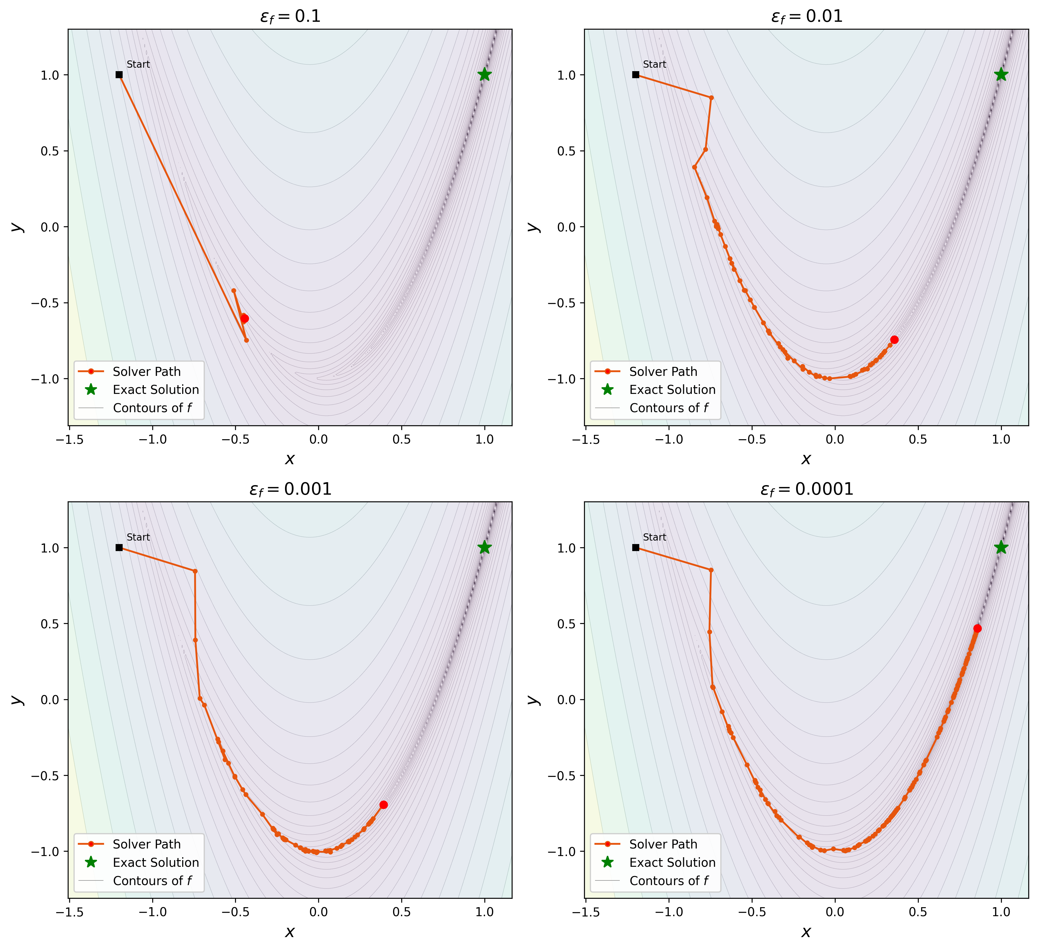
To further illustrate the behavior of the algorithm for this challenging objective, we plot in Figure 4 the iterate trajectories for the same runs using the noise levels $\epsilon_{f}\in\{10^{-1},10^{-2},10^{-3},10^{-4}\}$. For larger noise, the trajectory is relatively short as the algorithm stagnates due to the noise. It should be said, however, that the algorithm at least generates iterates that fall within the steep curved valley that contains the global minimizer, even though with high noise it is not able to navigate around the valley to the minimizer. As the noise decreases, however, the trajectories demonstrate better progress, approaching the behavior that one would expect in the noiseless setting.

Figure 4: Iterate trajectories for different noise levels $\epsilon_{f}$.

Overall, this experimental setup demonstrates that the method offers stable behavior and is robust to noise, with improved performance as $\epsilon_{f}$ decreases.

4.3 Neural Network Training for Binary Classification

To evaluate the performance of our proposed algorithm in a higher-dimensional setting, we considered a problem to train a neural network for binary classification using a dataset pertaining to the diagnosis of heart disease [27]. The dataset contains $1,026$ data points, each with $13$ features, along with a binary label indicating the presence or absence of heart disease. All features are normalized to have zero mean and unit variance. The model that we employed was a feed-forward neural network with a single hidden layer of size 10 and ReLU activation. The network outputs a single logit per sample, which is converted to a label probability via a sigmoid function. We employed the binary cross-entropy loss function. Due to the use of ReLU activation in the hidden layer, the resulting objective function is nonsmooth, in addition to being nonconvex.

For this challenging problem, we considered two experimental setups. The first represents an idealized setting in which values for the noise bounds $(\epsilon_{f},\epsilon_{g})$ are known explicitly. The second represents a more realistic scenario when the objective and generalized-gradient values are computed through mini-batching with a fixed mini-batch size and the noise bounds are not presumed to be known. In this latter case, we demonstrate the performance of the algorithm in terms of its dependence on $\epsilon_{\rm ls}$.

4.3.1 Adaptive Sampling

In this experiment, our main purpose is to demonstrate the trade-off between computational effort and final classification accuracy for different noise levels, assuming in each run that the noise levels are known. In order to run these experiments, in each iteration when the objective function or a generalized-gradient value is requested by the solver, the number of data points that are employed is increased adaptively until conditions on par with those in Assumptions 2.1 and 2.2 are found to hold. This represents an unrealistic scenario in which the true objective and gradient functions are evaluated explicitly. Thus, this experiment is for demonstration purposes only; a more realistic setup is considered in the following subsection.

More precisely, at each iteration, both the objective and gradient are estimated using a subset of data, starting from a small mini-batch. The mini-batch size is increased progressively until the desired accuracy conditions are satisfied, namely,

$$|f_{\text{mini-batch}}(x_{k})-f(x_{k})|\leq\epsilon_{f}\ \ \text{and}\ \ \|g_{\text{mini-batch}}(x_{k})-g(x_{k})\|_{2}\leq\epsilon_{g}:=\sqrt{\epsilon_{f}},$$

where $f(x_{k})$ and $g(x_{k})$ represent the objective function and gradient values that are computed using the entire set of data points and $f_{\text{mini-batch}}(x_{k})\equiv\tilde{f}(x_{k})$ and $g_{\text{mini-batch}}(x_{k})\equiv\tilde{g}(x_{k})$ are approximations obtained through mini-batch sampling.

To study the aforementioned trade-off between computational effort and classification accuracy, we run the algorithm for a range of $\epsilon_{f}$ values, recording both the total number of samples used throughout the optimization process and the final classification accuracy evaluated on the full dataset. For these experiments, we set stationary_tolerance of NonOpt to $10^{-8}$. The results are reported in Figure 5. We observe a clear trade-off between computational effort and solution quality. Smaller values of $\epsilon_{f}$ lead to more accurate gradient and objective estimates, resulting a higher final accuracy, but at the expense of significantly increased computational cost in terms of the total number of samples employed. Conversely, larger values of $\epsilon_{f}$ reduce the number of samples required, but lead to poorer solver performance and lower classification accuracy. It should be said that there exists an intermediate level (e.g., $\epsilon_{f}=0.05$), where the algorithm achieves high accuracy while using relatively fewer samples than the more exact setting.

Figure 5: Trade-off between total samples used throughout the optimization process (i.e., computational cost) and final classification accuracy as a function of the noise level.

Overall, these results demonstrate that the algorithm offers a balance between accuracy and computational effort in modern settings such as neural network training.

4.3.2 Fixed Mini-Batch Sampling

For a more realistic setting in which our algorithm may be applied in the context of machine learning, we next investigate the behavior of the algorithm in a fixed mini-batch-size setting. In our experiments here, the mini-batch size was fixed to 128 throughout the optimization process.

The same neural network architecture, dataset, and loss function as in the previous experiment were used. The only source of stochasticity arises from mini-batch sampling in each iteration. Here, we study the effect of the line-search parameter $\epsilon_{\rm ls}$, which controls the sufficient decrease condition in the backtracking procedure. This parameter effectively determines how strictly the algorithm enforces descent in the presence of noisy function and gradient estimates. In each iteration, we recorded:

1. the true objective value $f_{\text{true}}(x_{k})$ evaluated at $x_{k},$

2. the norm of the noisy/stochastic gradient evaluated at $x_{k}$,

3. the objective function error $\epsilon_{f,k}=|\tilde{f}(x_{k})-f_{\text{true}}(x_{k})|$, and

4. the gradient function error $\epsilon_{g,k}=|\tilde{g}(x_{k})-g_{\text{true}}(x_{k})|$.

We emphasize that $f_{\text{true}}$ and $g_{\text{true}}$ were only recorded in order to plot the results, and these quantities were not employed by the algorithm in any way. We ran the algorithm for $\epsilon_{\rm ls}\in\{10^{-3},10^{-2},10^{-1},1,10,100\}$, using $10^{-4}$ for the stationarity_tolerance in NonOpt. The results are shown in Figure 6.

Figure 6: Various metrics over iterations for different $\epsilon_{\rm ls}$ values. In the title of each plot, the final accuracy (“Acc.”) over the training dataset is recorded.

The results in Figure 6 illustrate the significant impact of the line-search parameter $\epsilon_{\rm ls}$ on the behavior of the algorithm when a fixed mini-batch sampling strategy is employed. (The faint background traces represent the raw, noisy values of the objective and gradient metrics at each iteration. To clearly illustrate the underlying convergence trends despite the stochastic fluctuations, the dotted lines represent a moving average calculated with a window size of 8 iterations.) For small values of $\epsilon_{\rm ls}$ (i.e., $10^{-3}$ and $10^{-2}$), the line-search condition is overly strict, causing the algorithm to make little progress due to frequent step rejections in the presence of stochastic noise. This results in nearly flat objective trajectories and relatively poor final accuracies between $48\%$ and $83\%$. (The discrepancy between these accuracies is due primarily to the randomness inherent in the algorithm terminating relatively early when minimizing the loss function, as is common in such settings.)

In contrast, moderate values of $\epsilon_{\rm ls}$ (i.e., 0.1, 1, and 10) yield stable behavior and better performance, achieving near-perfect to perfect classification accuracy (from $99.7\%$ to $100\%$). In these regimes, the condition $\epsilon_{\rm ls}>2\epsilon_{f}$ is regularly satisfied, as evidenced by the plotted values of $\epsilon_{f,k}$, which remain sufficiently small relative to $\epsilon_{\rm ls}$. However, when $\epsilon_{\rm ls}$ becomes too large (i.e., 100), the method becomes unstable, producing erratic objective and gradient behavior, larger estimation errors, and a drop in accuracy to about $93\%$, indicating that the algorithm allows steps that do not make reliable improvement in the true objective function.

Overall, these results highlight a fundamental trade-off: too small $\epsilon_{\rm ls}$ values lead to overly conservative updates and stagnation, while too large values cause instability, with intermediate values that satisfy the condition $\epsilon_{\rm ls}>2\epsilon_{f}$ offering the best compromise for robust and efficient optimization under stochastic noise.

5 Conclusion

We have proposed, analyzed, and tested an algorithm for solving nonconvex and nonsmooth optimization problems when both objective function and generalized-gradient evaluations may be corrupted by bounded, uncontrollable errors. To the best of our knowledge, ours is the first gradient-sampling-based method for solving problems in such a setting. We have proved reasonable convergence guarantees for our proposed algorithm, and demonstrated through multiple experiments that the algorithm is reliable and robust in the presence of noise, even when certain values required for the theoretical guarantees are not available in practice.

Our numerical experiments did not attempt to approximate a Lipschitz constant for the objective function despite the fact that a Lipschitz constant over a certain sublevel set is required for our theoretical guarantees. On one hand, setting a minimum step size to a very small value, such as $10^{-20}$ as is used in our experiments, would be consistent with our theoretical guarantees if the Lipschitz constant is not extremely large (i.e., if it is not large relative to $10^{20}$). On the other hand, in practice, it is possible that one might obtain better performance if the Lipschitz constant were known, or at least estimated during the optimization process, and in turn employed by the algorithm. One way of obtaining a rough approximation of the Lipschitz constant is to maintain a maximum value of $|\tilde{f}(x_{k})-\tilde{f}(x_{k+1})|/\|x_{k}-x_{k+1}\|_{2}$ over $k\in\mathbb{N}$. Such an approximation is reasonable as long as $\|x_{k}-x_{k+1}\|_{2}$ is large relative to $\epsilon_{f}$. Thus, one might ignore such values when $\|x_{k}-x_{k+1}\|_{2}$ is smaller than a user-defined threshold. Overall, we do not expect that such an estimation procedure would lead to huge benefits for the algorithm’s performance in practice. Rather, in our experience, the most important parameter is $\epsilon_{\rm ls}$, for which estimation techniques are well known.

References

- [1] (2019) Derivative-free optimization of noisy functions via quasi-newton methods. SIAM Journal on Optimization 29 (2), pp. 965–993. Cited by: §1.2, §2, §2.
- [2] (2022) Convergence of constant step stochastic gradient descent for non-smooth non-convex functions. Set-Valued and Variational Analysis 30 (3), pp. 1117–1147. Cited by: §1.2.
- [3] (2023) Subgradient sampling for nonsmooth nonconvex minimization. SIAM Journal on Optimization 33 (4), pp. 2542–2569. Cited by: §1.2.
- [4] (2018) Optimization methods for large-scale machine learning. SIAM Review 60 (2), pp. 223–311. Cited by: §1.2.
- [5] (2020) Gradient sampling methods for nonsmooth optimization. In Numerical Nonsmooth Optimization, pp. 201–225. Cited by: §1, §3.
- [6] (2005) A robust gradient sampling algorithm for nonsmooth, nonconvex optimization. SIAM Journal on Optimization 15 (3), pp. 751–779. Cited by: §1, 1st item.
- [7] (1983) Optimization and Nonsmooth Analysis. Canadian Mathematical Society Series of Monographs and Advanced Texts, John Wiley & Sons, New York, NY, USA. Cited by: §1.3, §1.3, §2.
- [8] (2022) Gradient sampling methods with inexact subproblem solutions and gradient aggregation. INFORMS Journal on Optimization 4 (4), pp. 347–445. Cited by: §1.
- [9] (2017) A BFGS-SQP method for nonsmooth, nonconvex, constrained optimization and its evaluation using relative minimization profiles. Optimization Methods and Software 32 (1), pp. 148–181. Cited by: §1.
- [10] (2012) A sequential quadratic programming algorithm for nonconvex, nonsmooth constrained optimization. SIAM Journal on Optimization 22 (2), pp. 474–500. Cited by: §1.
- [11] (2013) An adaptive gradient sampling algorithm for nonsmooth optimization. Optimization Methods and Software 28 (6), pp. 1302–1324. Cited by: §1, §4.1.
- [12] (2015) A quasi-Newton algorithm for nonconvex, nonsmooth optimization with global convergence guarantees. Mathematical Programming Computation 7 (4), pp. 399–428. Cited by: §1, §4.1.
- [13] (2020) A self-correcting variable-metric algorithm framework for nonsmooth optimization. IMA Journal of Numerical Analysis 40 (2), pp. 1154–1187. Cited by: §1.
- [14] (2025) Practical nonconvex nonsmooth optimization. MOS-SIAM Series on Optimization, Society for Industrial and Applied Mathematics, Philadelphia, PA, USA. Cited by: §1.3, §1.3, §2, §3, §3, §3.
- [15] (2025) NonOpt: Nonconvex, nonsmooth optimizer. Note: arXiv 2503.22826 Cited by: §4.1.
- [16] (2020) Stochastic subgradient method converges on tame functions. Foundations of Computational Mathematics 20 (1), pp. 119–154. Cited by: §1.2.
- [17] (2022) A gradient sampling method with complexity guarantees for lipschitz functions in high and low dimensions. In Advances in Neural Information Processing Systems, A. H. Oh, A. Agarwal, D. Belgrave, and K. Cho (Eds.), Cited by: §1.2.
- [18] (2019) Stochastic model-based minimization of weakly convex functions. SIAM Journal on Optimization 29 (1), pp. 207–239. Cited by: §1.2.
- [19] (2014) Convex proximal bundle methods in depth: a unified analysis for inexact oracles. Mathematical Programming 148 (1), pp. 241–277. Cited by: §1.2.
- [20] (1998) Stochastic generalized gradient method for nonconvex nonsmooth stochastic optimization. Cybernetics and Systems Analysis 34 (2), pp. 196–215. Cited by: §1.2.
- [21] (2015) Measure Theory and Fine Properties of Functions. Revised edition, Mathematics & Statistics, Chapman and Hall/CRC, New York, NY, USA. Cited by: §1.3.
- [22] (1977) Optimization of Lipschitz continuous functions. Mathematical Programming 13 (1), pp. 14–22. Cited by: §3.
- [23] (2012) On nesterov’s nonsmooth chebyshev–rosenbrock functions. Nonlinear Analysis: Theory, Methods and Applications 75 (3), pp. 1282–1289. Note: Variational Analysis and Its Applications Cited by: §4.2.
- [24] (2016) A proximal bundle method for nonsmooth nonconvex functions with inexact information. Computational Optimization and Applications 63 (1), pp. 1–28. Cited by: §1.2.
- [25] (2001) A proximal bundle method based on approximate subgradients. Computational Optimization and Applications 20 (3), pp. 245–266. Cited by: §1.2.
- [26] (2023) A redistributed proximal bundle method for nonsmooth nonconvex functions with inexact information. Journal of Industrial and Management Optimization 19 (12), pp. 8691–8708. Cited by: §1.2.
- [27] (1989) Heart Disease. Note: UCI Machine Learning RepositoryDOI: https://doi.org/10.24432/C52P4X Cited by: §4.3.
- [28] (2006) A proximal bundle method with approximate subgradient linearizations. SIAM Journal on optimization 16 (4), pp. 1007–1023. Cited by: §1.2.
- [29] (2007) Convergence of the gradient sampling algorithm for nonsmooth nonconvex optimization. SIAM Journal on Optimization 18 (2), pp. 379–388. Cited by: §1, §3.
- [30] (2010) The effect of deterministic noise in subgradient methods. Mathematical programming 125 (1), pp. 75–99. Cited by: §1.2.
- [31] (2013) Bundle method for non-convex minimization with inexact subgradients and function values. In Computational and Analytical Mathematics: In Honor of Jonathan Borwein’s 60th Birthday, pp. 555–592. Cited by: §1.2.
- [32] (1986) Stochastic generalized-differentiable functions in the problem of nonconvex nonsmooth stochastic optimization. Cybernetics 22 (6), pp. 804–809. Cited by: §1.2.
- [33] (2021) Stochastic generalized gradient methods for training nonconvex nonsmooth neural networks. Cybernetics and Systems Analysis 57 (5), pp. 714–729. Cited by: §1.2.
- [34] (1974) Minimization of nondifferentiable functions in the presence of noise. Cybernetics 10 (4), pp. 619–621. Cited by: §1.2.
- [35] (2023) Constrained optimization in the presence of noise. SIAM Journal on Optimization 33 (3), pp. 2118–2136. Cited by: §1.2, §2, §2.
- [36] (1919) Über partielle und totale differenzierbarkeit von Funktionen mehrerer Variabeln und über die Transformation der Doppelintegrale. Mathematische Annalen 79 (4), pp. 340–359. Cited by: §1.3.
- [37] (1998) Variational analysis. Grundlehren Der Mathematischen Wissenschaften, Vol. 317, Springer Berlin Heidelberg, Berlin, Heidelberg. Cited by: §1.3.
- [38] (2020) Convergence of a stochastic subgradient method with averaging for nonsmooth nonconvex constrained optimization. Optimization Letters 14 (7), pp. 1615–1625. Cited by: §1.2.
- [39] (2021) A stochastic subgradient method for nonsmooth nonconvex multilevel composition optimization. SIAM Journal on Control and Optimization 59 (3), pp. 2301–2320. Cited by: §1.2.
- [40] (1998) Error stability properties of generalized gradient-type algorithms. Journal of Optimization Theory and Applications 98 (3), pp. 663–680. Cited by: §1.2.
- [41] (2003) On approximations with finite precision in bundle methods for nonsmooth optimization. Journal of Optimization Theory and Applications 119 (1), pp. 151–165. Cited by: §1.2.
- [42] (2020) Complexity of finding stationary points of nonconvex nonsmooth functions. In International Conference on Machine Learning, pp. 11173–11182. Cited by: §1.2.