Variational Graph Neural Networks for Uncertainty Quantification in Inverse Problems

Abstract

The increasingly wide use of deep machine learning techniques in computational mechanics has significantly accelerated simulations of problems that were considered unapproachable just a few years ago. However, in critical applications such as Digital Twins for engineering or medicine, fast responses are not enough; reliable results must also be provided. In certain cases, traditional deterministic methods may not be optimal as they do not provide a measure of confidence in their predictions or results, especially in inverse problems where the solution may not be unique or the initial data may not be entirely reliable due to the presence of noise, for instance. Classic deep neural networks also lack a clear measure to quantify the uncertainty of their predictions. In this work, we present a variational graph neural network (VGNN) architecture that integrates variational layers into its architecture to model the probability distribution of weights. Unlike computationally expensive full Bayesian networks, our approach strategically introduces variational layers exclusively in the decoder, allowing us to estimate cognitive uncertainty and statistical uncertainty at a relatively lower cost.

In this work, we validate the proposed methodology in two cases of solid mechanics: the identification of the value of the elastic modulus with nonlinear distribution in a 2D elastic problem and the location and quantification of the loads applied to a 3D hyperelastic beam, in both cases using only the displacement field of each test as input data. The results show that the model not only recovers the physical parameters with high precision, but also provides confidence intervals consistent with the physics of the problem, as well as being able to locate the position of the applied load and estimate its value, giving a confidence interval for that experiment.

Keywords: Variational Inference, Graph Neural Networks, Inverse Problems, Hyperelasticity, Uncertainty Quantification.

1 Introduction

The most transformative aspects that today’s society is experiencing are undoubtedly the development and practical implementation of technologies applied to problems that just a few years ago were considered unfeasible due to cost or complexity (fast genomic sequencing; algorithms that predict the response to certain drugs; smart, personalized, and adaptive production). Without these technologies, precision medicine and industry, among others, would remain limited and applied to specific and undoubtedly costly cases. These phenomena have a common denominator, which is the ability to manage and exploit enormous volumes of data in real time for decision-making.

In particular, industry and precision medicine also share a need: to merge the physical world with the virtual world through digital twins [1]. To be effective, numerical simulation must be capable of delivering results in real time, a requirement that classical methods generally cannot meet due to their high computational cost.

Scientific Machine Learning has emerged as a promising solution. The development of artificial neural network architectures informed by physics (PINNs) [2], thermodynamics (TINNs) [3], or neural operators (DeepONet) [4] has demonstrated their ability to emulate complex physics at response speeds superior to those of classical solvers. However, the vast majority of these models are deterministic, meaning that given input data, they produce output data without informing the user about the reliability of that prediction.

This aspect can be considered critical in some inverse problems, where the aim is to obtain the causes that have generated certain effects, for example, to obtain the properties of the material that have produced certain displacements under a given load. It is well known that the nature of the input data (noised data) or the lack of uniqueness of the solution to the problem can lead to significant errors if one relies entirely on the prediction obtained with this type of architecture.

This paper proposes a hybrid architecture—combining the capabilities provided by the geometric biases of graph neural networks (GNNs) [5, 6, 7] with variational inference [8, 9]—which, in our point of view, overcomes the limitations of conventional networks by providing efficient quantification of uncertainty.

To do this, we use a combination of graph neural networks with variational layers that let us get a non-deterministic solution to the inverse problems posed, since it treats the weights of the network of these variational layers not as fixed values, but as random variables with a probability distribution. This allows our architecture to quantify two types of uncertainty: cognitive (or epistemic) uncertainty, which is the uncertainty associated with a lack of data or knowledge of the model—this type of uncertainty can be reduced with more data—; and statistical (or random) uncertainty, which is the uncertainty associated with the noise inherent in the input data.

There are two types of architectures that allow the probability distribution of weights to be processed. On the one hand, there are Bayesian neural networks (BNNs) [10], which, as mentioned above, go a step further than conventional neural networks by treating the network weights as random variables that follow a probability distribution, rather than obtaining fixed values for the weights.

The main objective of Bayesian inference in this context is to obtain the posterior distribution of the weights for some input data (training data). This is why BNNs can quantify the uncertainty in their predictions, making them particularly valuable in applications such as reliable uncertainty estimation or outlier detection.

However, training a BNN is computationally expensive. For this reason, approximate methods such as variational inference, among others, are used. This approach is widely used when working with very complex models or large data sets. Instead of calculating the probability distribution of the weights, variational inference seeks a simpler distribution that approximates it as closely as possible [11]. Variational neural networks incorporate variational inference directly into the architecture to model uncertainty, improve robustness, and encourage better generalization.

In summary, variational inference is a Bayesian technique that replaces complex and intractable posterior distributions with simpler distributions that are more efficient to optimize, which is the alternative used in this work.

As already mentioned, there is a neural PDE solver architecture that has demonstrated a great capacity to adapt to changes in geometry and boundary conditions: graph networks [12, 13]. Combined with a Bayesian variational approach to solving inverse problems, the resulting architecture promises to provide some very important features, particularly for the design of digital twins in changing environments [14, 15].

The purpose of this work is precisely to explore the possibilities offered by both methodologies: on the one hand, the quantification of uncertainty provided by the Bayesian approach to the problem. On the other hand, the generalisability of graph networks, already demonstrated in the literature. We thus hope that the result will be a technique with a high degree of generalisation in the face of changing scenarios and even those not seen in training.

The outline of the paper is as follows. In Section 2 we introduce the proposed architecture for our networks. Section 3 briefly introduces the strategy followed for training. Section 4 presents the chosen numerical examples that demonstrate the sought advantages of our approach. Finally, in Section 5 we draw some conclusions.

2 Neural Network Architecture

In computational mechanics, continuum models are discretized using usually unstructured meshes (triangles, tetrahedrons) to adapt to the complex geometries of the different problems under study. However, classical deep learning methods, such as convolutional neural networks (CNNs) that dominate image processing, operate on regular domains [16]. Projecting these meshes onto regular grids to use CNNs can introduce interpolation errors or loss of important topological information.

Graph Neural Networks (GNNs) generalize convolution to domains that are not necessarily regular [5, 6, 17, 18]. They treat the computational mesh of the model directly as if it were a graph $\mathcal{G}=(\mathcal{V},\mathcal{E})$, composed by a set of vertices $\mathcal{V}$ and edges $\mathcal{E}$, preserving the original connectivities and guaranteeing an indispensable physical property: it is invariant to the ordering of the nodes, i.e., the result does not depend on the order in which the nodes have been enumerated.

Graph networks employed as a neural Partial Differential Equation (PDE) solver classically follow the pattern proposed by Battaglia et al. [12] and consists of an encoder, a processor and a decoder, whose structure we describe next.

2.1 Encoder

The encoder processes the input data (dimension of a mesh node, processing all at once in the dimension reserved for the batch) and projects it onto the latent space of a higher dimension than the input one. Let $\boldsymbol{x}_{i}$ be the feature vector of node $i$. In this work, the coordinates and displacements (observable variables) of each node are considered. In order to characterize and differentiate each experiment or simulation to which this displacement field is attributed, the mean of this displacement field of the experiment is also taken into account. The characteristics of the edge are denoted by $\boldsymbol{a}_{ij}$, which in this work considers the relative distance between neighboring nodes (defined by the connectivity of the graph). The encoder consists of two independent multi-layer perceptron (MLP) networks for nodes and edges:

$$\boldsymbol{v}_{i}^{(l)}=f(\boldsymbol{W}_{v,l}\boldsymbol{x}_{i}+\boldsymbol{b}_{v,l}),\quad\boldsymbol{e}_{ij}^{(l)}=f(\boldsymbol{W}_{e,l}\boldsymbol{a}_{ij}+\boldsymbol{b}_{e,l}),$$ (1)

where $f$ is a nonlinear activation function. Specifically, in this work, the SwishLayer activation function has been used [19], and $l$ fully connected layers have been considered for each MLP, $l=1,\ldots,3$. The subscripts $i,j$ run through the number of nodes in the model.

2.2 Processor

The processor is the interaction core that performs $m$ message steps to propagate information across the domain using the connectivity defined in the graph. This is essential for simulating the physics of the problem, since local interactions between neighboring nodes give rise to global behaviors of the entire model. For each message step $k=1,\ldots,m$:

1. The information for each edge of the graph is updated by calculating the “message”—interaction value from the information stored in the connected nodes.

   $$\boldsymbol{e}_{ij}^{(k+1)}=\boldsymbol{e}_{ij}^{(k)}+\phi_{e}\left(\boldsymbol{v}_{i}^{(k)},\boldsymbol{v}_{j}^{(k)},\boldsymbol{e}_{ij}^{(k)}\right).$$ (2)

2. Message passing step, where

   $$m_{i}=\sum_{j\in\boldsymbol{N}(i)}\boldsymbol{e}_{ij}^{(k+1)}.$$

   The number of message passes is a key parameter in the performance of graph networks. In [20], the minimum number of message passes required to ensure a given level of prediction accuracy is studied in depth, depending on the type of partial differential equation governing the physical process.

3. Node aggregation and updating step. For each node, it aggregates the messages from its neighborhood $\boldsymbol{N}(i)$ and updates its state.

   $$\boldsymbol{v}_{i}^{(k+1)}=\boldsymbol{v}_{i}^{(k)}+\phi_{v}\left(\boldsymbol{v}_{i}^{(k)},m_{i}\right)=\boldsymbol{v}_{i}^{(k)}+\phi_{v}\left(\boldsymbol{v}_{i}^{(k)},\sum_{j\in\boldsymbol{N}(i)}\boldsymbol{e}_{ij}^{(k+1)}\right),$$ (3)

   where $\phi_{e}$ and $\phi_{v}$ are again basic neural networks (3-layer fully connected MLPs with swissLayer activation functions). It is important to note that the number of steps $m$ determines how much information each node receives. As discussed in [20], an insufficient $m$ causes the phenomenon known as under-reaching, where physical information does not have time to propagate throughout the domain (analogous to the CFL condition in explicit numerical methods), preventing or making convergence of the inverse problem more difficult.

2.3 Variational Decoder

Unlike Graph Networks, where all the weights calculated by the network are constant, and unlike Bayesian Networks, where all the weights in the network are distributions (which considerably increases the computational cost and significantly hinders the convergence of the network), in this work we propose a hybrid approach. The Encoder and Processor are deterministic, extracting deep features and therefore their weights are considered constant, and uncertainty is modeled only in the decoder, defining a Variational Decoder whose weights are probability distributions.

To solve the inverse problem, we seek the posterior distribution of the parameters to be estimated $\boldsymbol{y}$ (e.g., Young’s modulus, or the position and value of the load) given the input data or observations $\boldsymbol{x}$ (e.g., the displacement field from the experiment). In this work, we assume that the output follows a Normal distribution, so the network seeks to obtain the best weights to obtain the mean and variance that best approximate the solution of the training data, i.e.,

$$p(\boldsymbol{y}|\boldsymbol{x})=\mathcal{N}(\boldsymbol{y}|\boldsymbol{\mu}_{\theta}(\boldsymbol{x}),\text{diag}(\boldsymbol{\sigma}_{\theta}^{2}(\boldsymbol{x}))),$$ (4)

where $\theta$ represents the network weights. The proposed network architecture therefore has two outputs: one predicts the mean vector $\boldsymbol{\mu}$ and the other predicts its variance $\boldsymbol{\sigma}^{2}$, which represents the noise in the network predictions, ensuring a certain degree of numerical stability.

Fig. 1 shows a diagram of the network architecture proposed in this work. With this proposed architecture, non-deterministic behavior is considered only in the Decoder, allowing the Processor to learn complex physical characteristics in a deterministic and efficient manner.

The dimensions of the input vector required by the network are those of the displacement field of a single node—2D or 3D, depending on the problem—concatenated with the average displacement of the experiment—used as a global feature to identify and differentiate each experiment and which adds, again, 2 or 3 dimensions to the input vector—and the information regarding whether or not the node belongs to the contour using a binary variable.

Additionally, graph information is provided, describing the node’s neighborhood (its connections with neighboring nodes). Specifically, it requires the Euclidean distance between neighboring nodes in each spatial direction and the modulus of that distance. This structure also includes the global characteristic of the experiment –in this work, it has been considered sufficient to use only the mean of the displacements of the entire mesh.

Figure 1: A sketch of the Variational Graph Neural Network Architecture.

The output of the neural network returns the parameters of a normal distribution of the parameter studied for the input node: the mean and the variance. As an example, Fig. 1 shows the Young’s modulus obtained for the displacement field given at the input. It is important to emphasize that only the input data from a single node is required for the network input, and that the network returns the Young’s modulus of that node (its distribution). During the inference phase, when all the nodes of the mesh are processed simultaneously (taking advantage of the batch size), the complete distribution of the parameter throughout the model is obtained.

Precisely because it is a node-to-node approach that explicitly incorporates graph connectivity, the model allows inference to be performed on meshes other than those used during training. This property is inherent to Graph Neural Networks (GNN) and is one of the main reasons for their versatility in computational mechanics—and in other disciplines. However, it is important to note that if only meshes with a limited range of element sizes (edges) have been processed during training, performance is likely to decline significantly when inferring on meshes with elements of a size considerably different from those processed during the training phase, as the network will have learned physical patterns strongly associated with a specific spatial scale.

2.4 Loss Function

Based on Bayes’ theorem,

$$P(\theta|\mathcal{D})=\frac{P(\mathcal{D}|\theta)\cdot P(\theta)}{P(\mathcal{D})}\propto P(\mathcal{D}|\theta)\cdot P(\theta),$$ (5)

the posterior probability $P(\theta|\mathcal{D})$ could be calculated from the likelihood probability distribution $P(\mathcal{D}|\theta)$ and the prior probability $P(\theta)$. Therefore, $P(\theta|\mathcal{D})$ is obtained by normalizing $P(\mathcal{D}|\theta)\cdot P(\theta)$ so that it sums to 1.

$P(\mathcal{D}|\theta)$ reflects how the parameters of the neural network are updated based on the data. Therefore, it can be used to make new predictions for new data (inputs), which is known as Bayesian inference.

The denominator of Bayes’ Theorem, Eq. 5, is called Evidence and is a marginal distribution that measures the probability of the data according to the model, that is, it is a normalizing constant that guarantees that the Posterior distribution adds up to $1$. Therefore, it is possible to update the certainty about the weights ($\theta$) based on the data $\mathcal{D}$,

$$P(\mathcal{D})=\int P(\mathcal{D}|\theta)\cdot P(\theta)d\theta.$$ (6)

As mentioned above, due to the difficulty of calculating the posterior distribution $P(\theta|\mathcal{D})$, we want to approximate it with a variational distribution $Q(\theta)$ that is closest to the posterior and is represented by a small set of parameters, such as means and variances of a multivariate Gaussian distribution.

Now, how do we know that we are in the variational distribution closest to the true posterior distribution if we do not know what this distribution is like? The answer is by using the Kullback-Leibler divergence between the two distributions, $D_{KL}[Q(\theta)||P(\theta|\mathcal{D})]$. The divergence $D_{KL}$ is also known as information divergence, information gain, or relative entropy, and is a non-symmetric measure of the similarity or difference between two distribution functions.

To do this, we simply need to arrive at the expression for the Evidence Lower Bound (ELBO), which is a useful lower bound of $\log(p(\mathcal{D}|\theta))$ (Log-likelihood) of the observed data,

$$\underbrace{\log P(\mathcal{D})}_{\text{Evidence}}-\underbrace{D_{KL}[Q(\theta)||P(\theta|\mathcal{D})]}_{\text{Our Goal}}=\overbrace{\underbrace{\mathbb{E}_{Q}[\log P(\mathcal{D}|\theta)]}_{\text{Classification Loss}}-\underbrace{D_{KL}[Q(\theta|\mathcal{D})||P(\theta)]}_{\text{Regularization Loss}}}^{ELBO}.$$ (7)

Thus, we have converted an inference problem into an optimization problem. By optimizing ELBO, we maximize the evidence, that is, we minimize the divergence between $Q(\theta)$ and $P(\theta|\mathcal{D})$.

Training is performed by maximizing the Evidence Lower Bound (ELBO) [21]. For a dataset $\mathcal{D}$, the loss function to be minimized consists of two parts:

$$\mathcal{L}=\mathcal{L}_{\text{NLL}}+\beta\cdot\mathcal{L}_{\text{KL}},$$ (8)

where $\beta\in[0,1]$ minimizes the cost of each minibatch in the training process, since,

$$\beta_{i}=\frac{2^{M-i}}{2^{M}-1},$$ (9)

$\beta$ being a scaling factor for estimating the posterior distribution of weights with $\sum_{i}^{M}\beta_{i}=1.$

3 Training Methodology

The basis of this proposal is stochastic training of the neural network using Variational Inference, [22]. The aim is to approximate the true posterior distribution $P(w|\mathcal{D})$ of the weights ($w$) that best fit the data ($\mathcal{D}$). Finding this true distribution $P(w|\mathcal{D})$ can be highly difficult and costly, so another variational distribution $Q(\theta)$ parameterized by $\theta=(\mu,\sigma)$ is sought that best approximates the true $P(w|\mathcal{D})$.

3.1 Local Reparameterization

To enable backpropagation through random sampling, we use the Local Reparameterization Trick proposed for variational inference in [21]. The weights $w$ are expressed as:

$$w=\mu+\log(1+e^{\rho})\odot\epsilon,\quad\epsilon\sim\mathcal{N}(0,I),$$ (10)

that is, the standard deviation is $\sigma=\log(1+e^{\rho})$.

This reparameterization allows the use of stochastic gradient descent for variational inference, since it decouples the randomness represented by $\epsilon$ from the parameters to be learned $\theta=(\mu,\rho)$, allowing the calculation of stable gradients.

3.2 Variational Inference and ELBO

Since the calculation of the exact posterior distribution $P(w|\mathcal{D})$ is intractable, the Kullback-Leibler (KL) divergence between $Q(\theta)$ and $P(w|\mathcal{D})$ is minimized. As developed above and reflected in Eq. (7), this is equivalent to maximizing the Evidence Lower Bound (ELBO), or minimizing the Negative ELBO cost function, since the optimizers implemented in neural networks perform gradient descent optimally,

$$ELBO\equiv\mathcal{L}(\theta)=\mathbb{E}_{Q(\theta)}[\log P(\mathcal{D}|\theta)]-D_{KL}[Q(\theta)||P(\theta)],$$ (11)

where the first term measures the fit to the data given the model weights (likelihood) and the second term acts as a complexity-dependent regularizer (prior), measuring how much the model deviates from the initial assumptions.

Rewriting Eq. (11) and taking into account Eq. (8) above, where the loss function has been defined, it is determined that,

$$-ELBO=-l+\beta\cdot D_{KL}[Q(\theta)||P(\theta)].$$ (12)

On the one hand, we want to minimize the loss function known as Negative Log-Likelihood ($\mathcal{L}_{\text{NLL}}=-l$). This loss function measures the fitting error in the data, weighted by the predicted uncertainty. In other words, it estimates the probability of the network’s prediction given the actual values and sampling noise.

In this work, we have chosen to use the logarithm of a normal distribution as the probability density function, thus,

$$\log\mathcal{N}(\boldsymbol{x},\mu,\sigma)=-\frac{(\boldsymbol{x}-\mu)^{2}}{2\sigma_{i}^{2}}-\frac{1}{2}\log(2\pi)-\log(\sigma).$$ (13)

Therefore, we calculate Log-Likelihood as the logarithm of the probability of the data given in the model, which for a Gaussian output such as the one proposed would be equivalent to:

$$l=\mathbb{E}_{Q(\theta)}[\log P(\mathcal{D}|\theta)]\approx\sum_{i}\log P(\mathcal{D}|\theta_{i})=\sum_{i}\left(-\frac{||\boldsymbol{y}_{i}-\boldsymbol{\mu}_{i}||^{2}}{2\boldsymbol{\sigma}_{i}^{2}}-\frac{1}{2}\log(2\pi)-\log(\boldsymbol{\sigma}_{i})\right),$$ (14)

with $\boldsymbol{y}_{i}\in\mathcal{D}$. This term allows the neural network to reduce loss by reducing error ($\boldsymbol{y}\approx\boldsymbol{\mu}$) or increasing variance ($\boldsymbol{\sigma}$) if error is unavoidable. In other words, it allows the model to “admit” that it does not know the answer, which is known as statistical or random uncertainty.

The second term of Eq. (12) is the Kullback-Leibler divergence ($D_{KL}$) and is a regularizer of the weights—or latent distributions—, which helps to avoid overfitting.

In particular, the Kullback-Leibler divergence for discrete probability distributions is defined according to

$$D_{KL}[Q(\theta)||P(\theta)] =\sum_{i}Q(\theta_{i})\log\left(\frac{Q(\theta_{i})}{P(\theta_{i})}\right)$$

$$=\sum_{i}Q(\theta_{i})\log\left(\frac{1}{P(\theta_{i})}\right)-\sum_{i}Q(\theta_{i})\log\left(\frac{1}{Q(\theta_{i})}\right)$$ (15)

$$=\mathcal{H}(Q,P)-\mathcal{H}(Q)\cong\text{logPost}-\text{logPrior},$$

where $\mathcal{H}(Q,P)\cong\log(P(\theta))\equiv\text{logPost}$ is known as Cross-Entropy and $\mathcal{H}(Q)\cong\log(Q(\theta))\equiv\text{logPrior}$ as entropy.

Therefore, Eq. (12) can be rewritten as

$$-ELBO=-l+\beta\cdot\left(\text{logPost}-\text{logPrior}\right).$$ (16)

1

Entrada: Dataset $\mathcal{D}=\{(x_{n},y_{n})\}$, number of epochs $nEpoch$

Entrada: Prior Hyperparameters: $\pi_{w},\sigma_{1},\sigma_{2}$

Salida: Variational Parameters: $\theta^{*}=\{\mu,\rho\}$, $\sigma_{\text{noise}}$

2

1ex// Initialization

3 Initialize trainable parameters;

41exfor epoch $e\leftarrow 1$ to $nEpoch$ do

5    Shuffle $\mathcal{D}$ and divide in mini-batches $\mathcal{B}$

6    for each batch $b\in\mathcal{B}$ do

       // Forward step

7       Forward noise $\epsilon\sim\mathcal{N}(0,I)$

8       $\sigma\leftarrow\log(1+\exp(\rho))$

9       $w\leftarrow\mu+\sigma\odot\epsilon$

10       Prediction: $\hat{y}\leftarrow f_{\text{VGNN}}(x_{b};w)$

11      

      1ex// ELBO Loss

12       $\mathcal{L}_{\text{data}}=\sum\log\mathcal{N}(y_{b}|\hat{y},\sigma_{\text{noise}}^{2})$

13       $D_{KL}=\log Q(w|\theta)-\log P(w)$

14       $\mathcal{L}_{\text{total}}\leftarrow\beta\cdot D_{KL}-\mathcal{L}_{\text{data}}$

15      

      1ex// Optimization (Backward)

16       Gradients computation: $\nabla_{\theta}\mathcal{L},\nabla_{\sigma_{\text{noise}}}\mathcal{L}$

17       $\theta\leftarrow\text{Adam}(\theta,\nabla_{\theta})$

18       $\sigma_{\text{noise}}\leftarrow\text{Adam}(\sigma_{\text{noise}},\nabla_{\sigma_{\text{noise}}})$

19      

20    end for

21   

22 end for

23return $\mu,\rho,\sigma_{\text{noise}}$

Algorithm 1 Variational Graph NN Training

As reflected above in the implemented Algorithm 1, which is analogous to the one developed in [22], to calculate logPrior we use Scale Mixture Prior to calculate the probability $p(\theta)$. This distribution is a weighted sum (we have considered $\pi_{w}=\frac{1}{2}$) of two Gaussians centered at zero with different variances ($\sigma_{1}^{2},\sigma_{2}^{2}$),

$$p(\theta)=\prod_{j}\pi_{w}\mathcal{N}(\theta_{j},0,\sigma_{1}^{2})+(1-\pi_{w})\mathcal{N}(\theta_{j},0,\sigma_{2}^{2}),$$ (17)

that are considered hyperparameters of the network and that in this work have been considered learnable during the training process.

This approach encourages the calculation of sparse weights. It assigns a peaked/narrow distribution to weights that are expected to be close to zero or irrelevant, and a much wider distribution to those weights that are significant.

Therefore, the Cross-Entropy $\mathcal{H}(Q,P)\cong\log(P(\theta))$ is calculated using,

$$\begin{split}\text{logPrior}=&\sum_{all}\pi_{w}\log\mathcal{N}(\theta_{\text{weights}},0,\sigma_{1}^{2})+(1-\pi_{w})\log\mathcal{N}(\theta_{\text{weights}},0,\sigma_{2}^{2})\\ &+\pi_{w}\log\mathcal{N}(\theta_{\text{bias}},0,\sigma_{1}^{2})+(1-\pi_{w})\log\mathcal{N}(\theta_{\text{bias}},0,\sigma_{2}^{2}).\end{split}$$ (18)

Finally, to calculate logPost, Gaussian Variational Posterior is implemented as a diagonal Gaussian distribution. The weights $\theta$ are obtained from the standard Normal as discussed in Subsection 3.1. Therefore, the Entropy $\mathcal{H}(Q)=\mathcal{H}(Q,Q)\cong\log(Q(\theta))$ is calculated using,

$$\begin{split}\text{logPost}=&\sum_{\text{all}}\log\mathcal{N}(\theta_{\text{weights}},\mu_{\text{weights}}+\log(1+e^{\rho_{\text{weights}}})\cdot\epsilon_{\text{weights}},\log(1+e^{\rho_{\text{weights}}}))\\ +&\log\mathcal{N}(\theta_{\text{bias}},\mu_{\text{bias}}+\log(1+e^{\rho_{\text{bias}}})\cdot\epsilon_{\text{bias}},\log(1+e^{\rho_{\text{bias}}})).\end{split}$$ (19)

When maximizing the Evidence Lower Bound, a balance is desired between adjusting the data and not overfitting it.

3.3 Proposed Algorithm

The algorithm implemented in MATLAB for VGNN training is developed in Algorithm 1. This procedure ensures the convergence of the variational parameters and the estimation of data noise.

During training, the algorithm updates the weights and biases and the (global) sampling noise. This last parameter represents the noise in the network’s predictions and is a parameter that the network learns. Specifically, it will calculate the weights for each layer $\mu_{\text{weights}}$, $\rho_{\text{weights}}$, $\mu_{\text{bias}}$, $\rho_{\text{bias}}$, $\sigma_{1}$ and $\sigma_{2}$.

3.4 Neural Network Prediction

Once trained, the neural network will return a sample of the weights and biases $[w_{\text{weights}},w_{\text{bias}}]$ in the variational layers of the decoder, with values $\epsilon_{\text{weights}},\epsilon_{\text{bias}}\sim\mathcal{N}(0,1)$, according to,

$$w_{\text{weights}}=\mu_{\text{weights}}+\log(1+e^{\rho_{\text{weights}}})\cdot\epsilon_{\text{weights}},$$

$$w_{\text{bias}}=\mu_{\text{bias}}+\log(1+e^{\rho_{\text{bias}}})\cdot\epsilon_{\text{bias}}.$$

Therefore, the value predicted by the network will be

$$\boldsymbol{\mu}_{NN}=\boldsymbol{X}_{\text{newData}}\cdot\boldsymbol{w}_{\text{weights}}+\boldsymbol{w}_{\text{bias}}.$$

4 Numerical Examples

The VGNN architecture proposed for parameter estimation in inverse problems is applied to two numerical examples already described at the beginning of this work. The framework has been fully implemented in MATLAB using its Deep Learning Toolbox and executed on NVIDIA GeForce 4090RTX.

4.1 Estimation of the Elastic Modulus in a 2D Plate under Plane Stress

The first example in which the technique developed above is applied seeks to obtain Young’s modulus $E(x,y)$ at the nodes of a two-dimensional plate under plane stress, as shown in Figure 2.

This is a square domain with side length $L=1.0$, and the problem is considered dimensionless without loss of generality. The Dirichlet boundary conditions in $\Gamma_{u}$ are homogeneous in the horizontal direction, allowing vertical displacement at that boundary, except at the origin. The Neumann boundary $\Gamma_{t}$ is the right side of the plate, which is subjected to a tensile load $\sigma_{x}=1.5$.

Figure 2: 2D Plate with a nonlinear distribution of the elastic modulus under plane stress.

The behavior of the plate varies for each experiment since the expression of the Elastic Module varies, following a random LogNormal distribution, and whose expression is

$$E(x,y)=\alpha+\gamma\exp\left(g(x,y)\right),$$ (20)

$$g(x,y)\sim\mathcal{GP}\left(0,\exp\left(-\frac{||\boldsymbol{x}-\boldsymbol{x^{\prime}}||^{2}}{2l^{2}}\right)\right),$$ (21)

where $\alpha=\gamma=l=1$ have been used. As reflected in [23], from where the dataset was obtained, the database is published in a public repository https://github.com/NASA/pigans-material-ID.

For each randomly generated expression of the Elastic Modulus at each node in the domain ($25\times 25$ nodes), a displacement field $\boldsymbol{u}$ has been obtained. For illustrative purposes, Fig. 3 shows three simulations belonging to the dataset used in training the network.

Figure 3: Three examples of experiments used in neural network training. The first row represents the actual distribution of the Elastic Module, the next two rows represent the corresponding displacements –horizontal and vertical, respectively– for the behavior of the material represented in the initial row.

4.1.1 Specific training parameters

To ensure the reproducibility of the results, the hyperparameters used and the generation process are detailed below.

The initial dataset in the repository has a very high number of simulations. For the purposes of this work, $115$ simulations were used for training and $100$ for testing, which was considered sufficient to verify the validity of the proposed technique. All meshes are identical and the same load and boundary conditions were applied to them. Therefore, the associated graph does not vary and consists of $625$ nodes and $1825$ edges (it was considered appropriate to generate self-informed connectivity). The neural network used in this example has only 23 800 parameters, and the most important hyperparameters were as follows:

• An ${\tt nBatch}=2$ has been used. Although the neural network input consists of data from a single node, the entire simulation (at least) is entered in the batch direction. Therefore, a batch of $2$ means that the training is fed with $2$ complete simulations.

• Latent space dimension $25$ neurons.

• $5$ Message Passing steps ($m$).

• $\sigma_{1}=\frac{1}{\exp(1)}$ and $\sigma_{2}=\frac{1}{\exp(2)}$.

• As mentioned throughout the document, SwishLayer has been used as the activation function, which is preferable in this type of problem due to its smoothness compared to ReLU.

• The number of epochs used in training was ${\tt nEpoch}=4500$.

• As this is a static problem, where the neural network does not play a temporal integrator role and the input data is synthetic, it was not considered necessary to add noise to the data.

• Considering that the input has only one field, that of displacements, and that this field is essential data for the characterization of each experiment, it was not deemed necessary to normalize the input data.

• The Adam optimizer was chosen with an adaptive learning rate $lr=10^{-3}$ that changes with training. Specifically, a learning rate decay of $98\%$ every $700$ epochs was used.

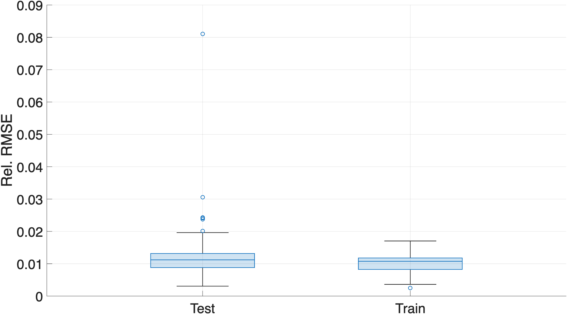
Fig. 4 shows the relative error (RRMSE) obtained for both the training and test datasets.

Figure 4: Relative RMSE error for training and test data for the problem of a 2D plate subjected to plane stress with nonlinear elastic modulus distributions.

Figures 5, 6, and 7 show the inference results for some of the test simulations, comparing the reference result—the actual distribution of the elastic modulus that leads to the displacement field used for the inference input—and the neural network prediction. It is important to note that, due to the architecture used in this work, the network also provides a confidence interval for the elastic modulus at each point. The figures showing the results reflect the lower and upper limits of the elastic modulus for each point.

Figure 5: Test example of the plate subjected to flat stress. The upper left shows the distribution of the actual elastic modulus (Ground Truth), while the upper right shows the average prediction of that field. The bottom row shows the lower and upper limits of that field, on the left and right, respectively.

Figure 6: Second test example of the plate subjected to plane stress. The upper left shows the distribution of the actual elastic modulus (Ground Truth), while the upper right shows the average prediction of that field. The bottom row shows the lower and upper limits of that field, on the left and right, respectively.

Figure 7: Third example test of the plate subjected to flat stress. The upper left shows the distribution of the actual elastic modulus (Ground Truth), while the upper right shows the average prediction of that field. The bottom row shows the lower and upper limits of that field, on the left and right, respectively.

The results show how the neural network is capable of effectively recovering the nonlinear distribution of Young’s modulus, as well as providing the distribution of uncertainty in the result offered, which allows us to see the areas of greater or lesser confidence in the results. A confidence interval of $97.72\%$ has been used in the representation of the results.

4.2 Estimation of the Load Applied to a 3D Hyperelastic Beam

In this second example, we seek to locate the position and value of the load applied to a cantilevered hyperelastic beam. The beam has Neo-Hookean behavior, with loads ranging from $F\in[5,100]kN$, every $5kN$ and at different positions on its upper face from the cantilevered end to an area near the fixed end, specifically linear loads at $13$ in the transverse direction and on the upper face. The dataset consists of $260$ high-fidelity simulations performed using the finite element method with nonlinear behavior of the hyperelastic beam with dimensions $40\times 10\times 10$. All meshes are identical, so the only difference between each simulation is the position and value of the applied load, which induces a displacement field that will be the data feeding the neural network training. All simulations have the same boundary and material conditions. For all the above reasons, the associated graph (Fig. 8) does not vary and consists of $240$ nodes and $824$ edges (it has been considered appropriate to generate self-informed connectivity) in a three-dimensional distribution.

Figure 8: Mesh (left) and graph (right) associated with the hyperelastic beam problem.

4.2.1 Training parameters

The neural network used in this example has only $6900$ parameters, and the most important hyperparameters have been the following:

• Once again, an ${\tt nBatch}=2$ has been used, which corresponds to $2$ simulations of the entire mesh, for a single load value. However, as has been emphasized throughout this work, the neural network input consists of data from a single node, and it is in the batch direction where two complete simulations are introduced in this case.

• Latent space dimension $12$ neurons.

• $4$ Message Passing ($m$) steps.

• SwishLayer has been used as the activation function.

• The number of epochs used in training has been ${\tt nEpoch}=5000$.

• It was not considered necessary to add noise to the data, nor was it deemed necessary to normalize the input data.

• The Adam optimizer was chosen with an adaptive learning rate $lr=10^{-3}$ that changes with training. Specifically, a Learning Rate decay of $98\%$ every $1000$ epochs was used.

Fig. 9 shows the relative error (RRMSE) obtained for both the training and test datasets.

Figure 9: Relative RMSE error for training and test data for the 3D Hyperelastic Beam problem.

In the following Figs. 10, 11, and 12 show the inference results for three of the test simulations, comparing the reference result—the actual value and position of the load applied to the beam, which leads to the displacement field used for the inference input and represented along the beam—with the predictions generated by the neural network. For each experiment, the average value of the load at each node is represented. Since this value is zero or almost zero at most nodes, it will not be reflected in the result, as the vectors are shown relative to their modulus. Again, the network also provides a confidence interval for the value of this load at every point in the domain.

Figure 10: Test example of the hyperelastic beam subjected to bending. The upper left shows the distribution of the applied load (ground truth) together with the displacement field that serves as input to the neural network, while the upper right shows the average prediction of the load value and its location. The bottom row shows the lower and upper limits of the load value distributions, on the left and right, respectively.

Figure 11: Second test example of the hyperelastic beam subjected to bending. The upper left shows the distribution of the applied load (Ground Truth) together with the displacement field that serves as input to the neural network, while the upper right shows the average prediction of the load value and its location. The bottom row shows the lower and upper limits of the load value distributions, on the left and right, respectively.

Figure 12: Third test example of the hyperelastic beam subjected to bending. The upper left shows the distribution of the applied load (Ground Truth) together with the displacement field that serves as input to the neural network, while the upper right shows the average prediction of the load value and its location. The bottom row shows the lower and upper limits of the load value distributions, on the left and right, respectively.

The uncertainty in the position of the load increases significantly as it approaches the Dirichlet boundary. This is consistent, since a force near the support produces very small displacements, which complicates the inverse problem.

Where a deterministic model would simply fail, the use of this architecture (VGNN) allows the user to be alerted by high variance.

4.3 Estimation of the Load Applied to a previously unseen Beam

In this last example, the training of the previous hyperelastic beam has been used to estimate the value and position of the load on a new beam, with a different geometry to that trained in the previous Section 4.2. Fig. 13 compares the geometry of the beam used to train the neural network with the new (shorter) beam for which the load is to be predicted.

Figure 13: Comparative of geometries of trained beam and the new, shorter one.

Fig. 14 shows the relative error in the prediction of $10$ new experiments, in which the value and position of the load are changed.

Figure 14: Relative RMSE error for test data for the new (shorter) 3D hyperelastic Beam problem.

In the following Figs.15, 16 and 17 show the inference results for three of the test simulations for not trained geometry, comparing the reference value and position of the load applied to the new beam, which leads to the displacement field used for the inference input and represented along the beam, with the predictions generated by the neural network. Again, for each experiment, the average value of the load at each node is represented. As previous examples, the network also provides a confidence interval for the value of this load at every point in the domain.

Figure 15: Test example of the new hyperelastic beam subjected to bending. The upper left shows the distribution of the applied load (Ground Truth) together with the displacement field that serves as input to the neural network, while the upper right shows the average prediction of the load value and its location. The bottom row shows the lower and upper limits of the load value distributions, on the left and right, respectively.

Figure 16: Test example of the new hyperelastic beam subjected to bending. The upper left shows the distribution of the applied load (Ground Truth) together with the displacement field that serves as input to the neural network, while the upper right shows the average prediction of the load value and its location. The bottom row shows the lower and upper limits of the load value distributions, on the left and right, respectively.

Figure 17: Test example of the new hyperelastic beam subjected to bending. The upper left shows the distribution of the applied load (Ground Truth) together with the displacement field that serves as input to the neural network, while the upper right shows the average prediction of the load value and its location. The bottom row shows the lower and upper limits of the load value distributions, on the left and right, respectively.

5 Conclusions

The implementation of Variational layers in Graph architectures allows for robust estimation of uncertainty thanks to the variational nature of the neural network without sacrificing the predictive and versatile performance offered by graph networks. The training algorithm presented effectively balances model complexity (KL divergence) and accuracy (likelihood), providing a valuable tool for complex problems where risk must be controlled.

The methodology developed in this work maintains the fundamental characteristics of GNNs by respecting the topology of the meshes of the proposed problems. The variational formulation in the decoder allows real-time confidence metrics to be obtained, and its application in quantifying uncertainty in nonlinear inverse problems confirms the robustness of the method.

References

- [1] Francisco Chinesta, Fouad El Khaldi, and Elias Cueto. Hybrid twin: an intimate alliance of knowledge and data. In The Digital Twin, pages 279–298. Springer, 2023.
- [2] M. Raissi, P. Perdikaris, and G.E. Karniadakis. Physics-informed neural networks: A deep learning framework for solving forward and inverse problems involving nonlinear partial differential equations. Journal of Computational Physics, 378:686–707, 2019.
- [3] Quercus Hernández, Alberto Badías, Francisco Chinesta, and Elías Cueto. Thermodynamics-informed graph neural networks. IEEE Transactions on Artificial Intelligence, 5(3):967–976, 2022.
- [4] Sifan Wang, Hanwen Wang, and Paris Perdikaris. Learning the solution operator of parametric partial differential equations with physics-informed deeponets. Science advances, 7(40):eabi8605, 2021.
- [5] Gabriele Corso, Hannes Stark, Stefanie Jegelka, Tommi Jaakkola, and Regina Barzilay. Graph neural networks. Nature Reviews Methods Primers, 4(1):17, 2024.
- [6] Federico Pichi, Beatriz Moya, and Jan S Hesthaven. A graph convolutional autoencoder approach to model order reduction for parametrized pdes. Journal of Computational Physics, 501:112762, 2024.
- [7] Alicia Tierz, Iciar Alfaro, David González, Francisco Chinesta, and Elías Cueto. Graph neural networks informed locally by thermodynamics. Engineering Applications of Artificial Intelligence, 144:110108, 2025.
- [8] Alex Graves. Practical variational inference for neural networks. Advances in neural information processing systems, 24, 2011.
- [9] Lucas Pinheiro Cinelli, Matheus Araújo Marins, Eduardo Antúnio Barros da Silva, and Sérgio Lima Netto. Variational autoencoder. In Variational methods for machine learning with applications to deep networks, pages 111–149. Springer, 2021.
- [10] Igor Kononenko. Bayesian neural networks. Biological Cybernetics, 61(5):361–370, 1989.
- [11] Cheng Zhang, Judith Bütepage, Hedvig Kjellström, and Stephan Mandt. Advances in variational inference. IEEE transactions on pattern analysis and machine intelligence, 41(8):2008–2026, 2018.
- [12] Peter W Battaglia, Jessica B Hamrick, Victor Bapst, Alvaro Sanchez-Gonzalez, Vinicius Zambaldi, Mateusz Malinowski, Andrea Tacchetti, David Raposo, Adam Santoro, Ryan Faulkner, et al. Relational inductive biases, deep learning, and graph networks. arXiv preprint arXiv:1806.01261, 2018.
- [13] Alicia Tierz, Mikel M Iparraguirre, Icíar Alfaro, David González, Francisco Chinesta, and Elías Cueto. On the feasibility of foundational models for the simulation of physical phenomena. International Journal for Numerical Methods in Engineering, 126(6):e70027, 2025.
- [14] M Gorpinich, B Moya, S Rodriguez, F Meraghni, Y Jaafra, A Briot, M Henner, R Leon, and F Chinesta. Bridging data and physics: A graph neural network-based hybrid twin framework. arXiv preprint arXiv:2512.15767, 2025.
- [15] Beatriz Moya, Alberto Badías, Icíar Alfaro, Francisco Chinesta, and Elías Cueto. Digital twins that learn and correct themselves. International Journal for Numerical Methods in Engineering, 123(13):3034–3044, 2022.
- [16] Pierre Sermanet, Soumith Chintala, and Yann LeCun. Convolutional neural networks applied to house numbers digit classification. In Proceedings of the 21st international conference on pattern recognition (ICPR2012), pages 3288–3291. IEEE, 2012.
- [17] Alvaro Sanchez-Gonzalez, Jonathan Godwin, Tobias Pfaff, Rex Ying, Jure Leskovec, and Peter Battaglia. Learning to simulate complex physics with graph networks. In Hal Daume and Aarti Singh, editors, Proceedings of the 37th International Conference on Machine Learning, volume 119 of Proceedings of Machine Learning Research, pages 8459–8468. PMLR, 13–18 Jul 2020.
- [18] Tobias Pfaff, Meire Fortunato, Alvaro Sanchez-Gonzalez, and Peter W. Battaglia. Meshgraphnets: Learning the physics of complex systems. Proceedings of the International Conference on Learning Representations (ICLR), 2021.
- [19] Prajit Ramachandran, Barret Zoph, and Quoc V Le. Searching for activation functions. arXiv preprint arXiv:1710.05941, 2017.
- [20] Lucas Tesan, Mikel M. Iparraguirre, David Gonzalez, Pedro Martins, and Elias Cueto. On the Under-Reaching Phenomenon in Message Passing Neural PDE Solvers: Revisiting the CFL Condition. Computer Methods in Applied Mechanics and Engineering, 449:118476, 2026.
- [21] Diederik P Kingma and Max Welling. Auto-encoding variational bayes. arXiv preprint arXiv:1312.6114, 2013.
- [22] Charles Blundell, Julien Cornebise, Koray Kavukcuoglu, and Daan Wierstra. Weight uncertainty in neural network. In International conference on machine learning, pages 1613–1622. PMLR, 2015.
- [23] James E Warner, Julian Cuevas, Geoffrey F Bomarito, Patrick E Leser, and William P Leser. Inverse estimation of elastic modulus using physics-informed generative adversarial networks. arXiv preprint arXiv:2006.05791, 2020.