Exact Skin Critical Phase and Configurable Fractal Wavefunctions via Imaginary Gauge Phase Imprint in Non-Hermitian Lattices

Abstract

The generation of complex states like multifractal critical states has been an outstanding challenge in both classical and quantum physics. Here we propose a general framework, termed the imaginary gauge phase imprint, allowing to engineer rigorous wavefunctions in any-dimensional non-Hermitian lattices. Using this method, we uncover a novel phase with exact critical wavefunctions in one (and two) dimension, dubbed the skin critical phase (SCP). Unlike conventional critical phases with overall uniform density distributions and non-Hermitian skin effect with eigenstate accumulation at open boundaries, the SCP is marked by a macroscopically multifractal distribution with all critical eigenstates sharing an identical profile and always accumulating at specific bulk interfaces under periodic boundary condition, which become topology-dependent boundary or interface skin modes under open boundary condition. We also show the ballistic dynamics in the SCP, in contrast to the diffusive behaviour in conventional critical phases. Moreover, we validate our method by imprinting configurable wavefunctions in higher dimensions, including complex fractal states with Sierpiński-carpet and Koch-snowflake profiles in non-fractal lattices and Moiré states in non-Moiré lattices. Our work not only offers fresh insights into fractal phenomena and critical phases, but also provides a rigorous paradigm for wave manipulations in engineered non-Hermitian systems.

Introduction— Fractals, describing self-similar geometric patterns, have a significant impact on various fields of modern physics, ranging from quasicrystals and critical phenomena to quantum spacetime [33, 18, 19, 5, 10]. In quasiperiodic systems, such as the paradigmatic Aubry-André (AA) model [2] and Moiré lattices [55, 70, 50], the single-particle energy spectrum exhibits fractal structures [31, 67]. The multifractality of wavefunctions also exhibits for critical states, which are fundamentally different from extended and localized states in localization physics [1, 35]. The multifractal critical states were firstly found at extended-localized transition points [2, 18], and now have been identified in the critical phase in quasiperiodic systems [26, 11, 45, 68, 78]. The critical phase with multifractal states enriches the localization and fractal phemomena [77, 72, 71, 24, 47, 73, 40, 90], but it is challenging to rigorously confirm critical states and separate them from extended and localized states in finite-size systems. Notably, the precise phase boundaries of critical states and corresponding transition energies have been determined in several exactly solvable 1D quasiperiodic models [89, 23, 22, 3]. Increasing experimental efforts have also been devoted to probing critical phases [59, 21, 76, 37, 62, 41, 32].

Recent research has significantly expanded localization physics in non-Hermitian systems [4, 81, 6], such as delocalization and erratic localization induced by imaginary gauge potentials [28, 29, 48, 53] and the non-Hermitian skin effect (NHSE) [79, 36, 34, 56, 7, 84, 38, 44]. The fractal spectrum can exhibit in complex energy plane in non-Hermitian quasiperiodic and fractal lattices [69, 64]. The 1D critical states therein have also been explored, which share common critical features with their Hermitian counterparts but exhibit boundary- or size-dependent localization [65, 9, 39, 46, 42]. Despite these advances on low-dimensional critical states, to our knowledge, there have not been exact wavefunctions for rigorously identifying critical phases in both Hermitian and non-Hermitian quasiperiodic systems in the thermodynamic limit. Moreover, two key open questions remain: Are there new types of critical phases in non-Hermitian systems? Can we realize configurable multifractal states in high dimensions?

In this Letter, we address these challenges by proposing a general framework, termed the imaginary gauge phase imprint, which allows to obtain exact wavefunctions in any-dimensional non-Hermitian lattices. Using this rigorous method, we reveal critical states with complex fractal structures, as shown in Fig. 1. Notably, we uncover an exotic phase, namely the skin critical phase (SCP), which has different static, dynamical, and skin characteristics from those for both conventional critical phase (CCP) [26, 11, 45, 68, 78, 65, 9, 39, 46, 42] and NHSE [79, 36, 34, 56, 7, 84, 38, 44], as summarized in Fig. 2(e). Furthermore, we validate our method by imprinting configurable wavefunctions in higher dimensions, including fractal states with Sierpiński-carpet or Koch-snowflake profiles in non-fractal lattices and Moiré states in non-Moiré lattices. Our work with exact solutions offers fresh insights into fractal phenomena and critical phases, and establishes a general paradigm for wave manipulations in engineered non-Hermitian systems.

Exactly solvable model and imaginary phase imprint.—We consider a generalized non-Hermitian Hatano-Nelson model [28, 29] with a spatially varying imaginary gauge phase [15, 87, 52, 48] in a $d$-dimensional simple lattice of size $N=L^{d}$ (with $L$ being the length along each direction), described by the tight-binding Hamiltonian

$$\hat{H}=\sum_{\alpha=1}^{d}\sum_{\mathbf{r}}J\left[e^{-g_{\mathbf{r}}^{(\alpha)}}\hat{c}_{\mathbf{r}}^{\dagger}\hat{c}_{\mathbf{r}+\mathbf{e}_{\alpha}}+e^{g_{\mathbf{r}}^{(\alpha)}}\hat{c}_{\mathbf{r}+\mathbf{e}_{\alpha}}^{\dagger}\hat{c}_{\mathbf{r}}\right]+\hat{H}_{B}.$$ (1)

Here, $\hat{c}_{\mathbf{r}}^{\dagger}$ ($\hat{c}_{\mathbf{r}}$) denotes the creation (annihilation) operator at lattice site $\mathbf{r}$, $\mathbf{e}_{\alpha}$ is the unit vector along $\alpha$ direction, $J$ is the hopping strength, and $g_{\mathbf{r}}^{(\alpha)}$ represents imaginary gauge phases that generally depend on site $\mathbf{r}$ and nonreciprocal hopping direction $\alpha$. Hereafter, we set $J=\hbar=1$ and $\hbar/J=1$ as the energy and time unit, respectively.

In 1D case of $d=\alpha=1$, one can rewrite $g_{\mathbf{r}}^{(1)}\equiv g_{n}$ with the site $n=1,2,...,L$. For higher dimensions $d\geqslant 2$, we first focus on the degenerated case that $g_{\mathbf{r}}^{(\alpha)}$ for each $\alpha$ direction just varies with the sites along this direction $r_{\alpha}\in[1,L]$ as $g_{\mathbf{r}}^{(\alpha)}\mapsto g_{r_{\alpha}}^{(\alpha)}$, and consider other general cases latter. $\hat{H}_{B}$ controls the boundary condition: $\hat{H}_{B}=0$ for the OBC, whereas for the PBC, $\hat{H}_{B}$ preserves nonreciprocal hopping between two boundary sites along each direction (see Supplemental Material (SM)). In the degenerated case, the single-particle eigen-equation derived from the Hamiltonian (1) is

$$E\psi_{\mathbf{r}}=\sum_{\alpha=1}^{d}J\left(e^{g_{r_{\alpha}-1}^{(\alpha)}}\psi_{\mathbf{r}-\mathbf{e}_{\alpha}}+e^{-g_{r_{\alpha}}^{(\alpha)}}\psi_{\mathbf{r}+\mathbf{e}_{\alpha}}\right),$$ (2)

where $\psi_{\mathbf{r}}$ and $E$ are the eigenstate and eigenenergy.

By an imaginary gauge transformation [52, 48]: $\psi_{\mathbf{r}}=\phi_{\mathbf{r}}\exp\left(\sum_{\alpha=1}^{d}X_{r_{\alpha}}^{(\alpha)}\right)$, where $X_{r_{\alpha}}^{(\alpha)}=\sum_{l=1}^{r_{\alpha}-1}g_{l}^{(\alpha)}$ is the total imaginary phase accumulated by the hopping along $\alpha$ direction, the gauge phase can be eliminated.

Figure 1: Imprinting exact multifractal critical states. (a) 1D critical state $|\psi_{n}|$ with the self-similar structure under imaginary phase $X_{n}$. (b) 2D critical state $|\psi_{n,m}|$ and (c) 3D critical state $|\psi_{n,m,p}|$ with Sierpiński-carpet fractal profiles, under imaginary phases $S_{n,m}$ and $V_{n,m,p}$, respectively. (d) Large-size scaling to extract the fractal dimension $D_{f}=0.605,1.939,2.884$ for critical states in (a-c), with system size $N=L^{d}>2.5\times 10^{9}$ sites.

This leads to a transformation of the non-Hermitian eigen-equation (2) into its equivalent Hermitian form: $E\phi_{\mathbf{r}}=\sum_{\alpha=1}^{d}J\left(\phi_{\mathbf{r}-\mathbf{e}_{\alpha}}+\phi_{\mathbf{r}+\mathbf{e}_{\alpha}}\right)$, which allows exact solutions via separation of variables along all directions. Letting $\phi_{\mathbf{r}}=\prod_{\alpha=1}^{d}\phi^{(\alpha)}_{r_{\alpha}}$ and $E=\sum_{\alpha=1}^{d}E^{(\alpha)}$, we obtain independent 1D equations along each direction $E^{(\alpha)}\phi^{(\alpha)}_{r_{\alpha}}=J(\phi^{(\alpha)}_{r_{\alpha}-1}+\phi^{(\alpha)}_{r_{\alpha}+1})$, where $\phi^{(\alpha)}_{0}=\phi^{(\alpha)}_{L_{\alpha}+1}=0$ for the OBC and $\phi^{(\alpha)}_{r_{\alpha}+L}=\phi^{(\alpha)}_{r_{\alpha}}\exp(-X_{L+1})=\phi^{(\alpha)}_{r_{\alpha}}\exp(-\bar{g}^{(\alpha)}L)$ for the PBC, with $\bar{g}^{(\alpha)}=\frac{1}{L}\sum_{l=1}^{L}g_{l}^{(\alpha)}$. By analytically solving these equations and applying the inverse gauge transformation, we obtain exact solutions of the model Hamiltonian (see the SM):

$$\psi_{\mathbf{r}}^{\{j^{(\alpha)}\}}=\begin{cases}\prod_{\alpha=1}^{d}\sin[\pi j^{(\alpha)}r_{\alpha}/(L+1)]e^{X_{r_{\alpha}}^{(\alpha)}},&\text{OBC};\\[8.61108pt] \prod_{\alpha=1}^{d}e^{i2\pi j^{(\alpha)}r_{\alpha}/L-\bar{g}^{(\alpha)}r_{\alpha}+X_{r_{\alpha}}^{(\alpha)}},&\text{PBC},\end{cases}$$ (3)

up to a normalization constant, where $\{j^{(\alpha)}\}$ with $j^{(\alpha)}=1,2,\dots,L$ denotes the eigenstate index with total number $N=L^{d}$. The corresponding eigenenergies are $E_{\text{OBC}}^{\{j^{(\alpha)}\}}=\sum_{\alpha=1}^{d}2J\cos[\pi j^{(\alpha)}/(L+1)]$ and $E_{\text{PBC}}^{\{j^{(\alpha)}\}}=\sum_{\alpha=1}^{d}2J\cos[2\pi j^{(\alpha)}/L+i\bar{g}^{(\alpha)}]$. For exact wavefunctions given by Eq. (3), a key observation is the phase profile $X_{r_{\alpha}}^{(\alpha)}$ controlled by the imaginary gauge phase $g_{r_{\alpha}}^{(\alpha)}$. This provides a versatile method to engineer eigenstate profiles in non-Hermitian lattices through designing and imprinting the imaginary gauge phase, similar to the real phase imprint for wavefunction engineering of atomic gases [8, 17, 16]. Thus, such an imaginary phase imprint method can be used to create exact multifractal critical states in any dimension, as shown in Fig. 1.

Figure 2: SCP in 1D. (a) Phase diagram on the $W$-$h$ plane. The system exhibits the SCP below the diagonal (grey dashed line) and extended phase in the striped region above. In the SCP, all eigenstates are skinned to bulk interfaces (Int) under the PBC for any $\omega$; while under the OBC, they become interface, left (L) or right (R) boundary skin modes for $\omega=0,1,-1$, respectively. The orange and blue shading regions has $\omega=\pm 1$ for $\bar{g}<0$ and $\bar{g}>0$, separating by exact boundaries as blue and red dashed lines with $\omega=\bar{g}=0$. (b) $\omega$ and $D_{f}$ as functions of $W$ with $h=1.25$. (c) Wavefunction distributions $|\psi_{n}|$ under the PBC and OBC for $\omega=0$ ($W=2$ and $h=1$) and $\omega=1$ ($W=1.5$ and $h=1$). (d) Corresponding $X_{n}$ (blue lines) and $X_{n}-\bar{g}n$ (red line) with quasiperiodic fluctuations and interfaces (green dash lines). (e) Expansion dynamics with time-evolved density profiles $\log P(n,t)$ in the SCP ($\bar{g}=0$ and $\bar{g}<0$) and the extended (Ext) phase from top to bottom panels). (f) Corresponding time-evolved second moment $M_{2}(t)$ with ballistic scaling $\delta=1$. The simulated $M_{2}(t)$ at the critical point of the AA model with diffusive scaling $\delta=0.5$ is shown for comparison. (g) Summary of properties of the CCP and SCP.

SCP in 1D.—For clarity, we here focus on the 1D case and discuss other cases later and in the SM. In Fig. 1(a), we show the self-similar fractal structure of a 1D critical state obtained via the imaginary phase imprint $X_{r_{\alpha}}^{(\alpha)}\doteq X_{n}=\sum_{l=1}^{n-1}g_{l}$ with the following imaginary gauge phase

$$g_{n}=\ln(|W\cos(2\pi\beta n+\varphi)+h\cos(\pi n)|).$$ (4)

Here, $\beta=(\sqrt{5}-1)/2$ is an irrational number, $W$ and $h$ are the strengths of the quasiperiodic and periodic modulations of the imaginary gauge phase, respectively, and $\varphi$ is a sampling phase. The exact wavefunction of the $j$-th ($j^{(\alpha)}\doteq j$ with $j=1,2,...,L$) eigenstate is given by

$$\psi_{n}^{(j)}=\begin{cases}\sin\left({\pi jn}/{(L+1)}\right)\exp\left(X_{n}\right),\quad\text{OBC};\\ \exp\left(i{2\pi jn}/{L}-\bar{g}n+X_{n}\right),\quad\text{PBC},\end{cases}$$ (5)

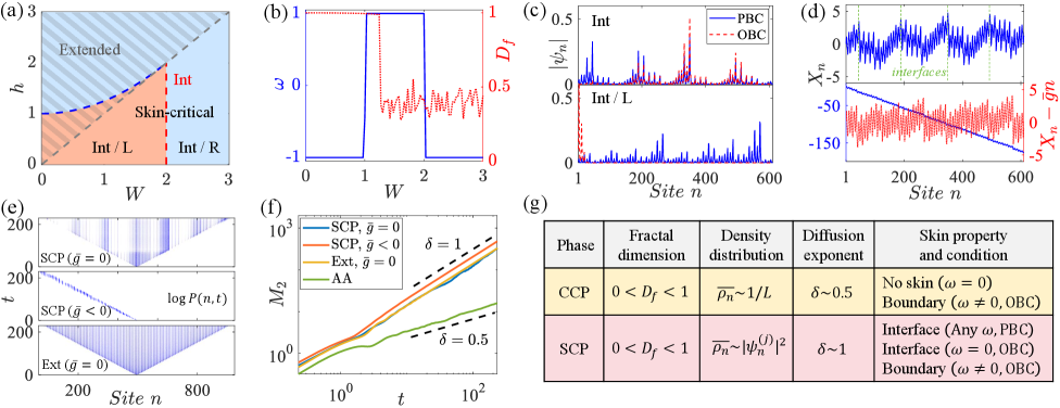
with $\bar{g}=\frac{1}{L}\sum_{n=1}^{L}g_{n}$ as the mean gauge field per lattice site, and eigenenergies $E_{\text{OBC}}^{(j)}=2J\cos\left({\pi j}/{(L+1})\right)$ and $E_{\text{PBC}}^{(j)}=2J\cos\left(2\pi j/L+i\bar{g}\right)$. The energy spectrum is real for the OBC, while for the PBC, it is complex and forms an elliptical loop satisfying $(\text{Re}[E_{\text{PBC}}^{(j)}])^{2}/\cosh^{2}\bar{g}+(\text{Im}[E_{\text{PBC}}^{(j)}])^{2}/\sinh^{2}\bar{g}=4J^{2}$. The spectral topology is characterized by the winding number of the loop of $E_{\text{PBC}}(k)=2J\cos\left(k+i\bar{g}\right)$ around the interior point $E_{\text{OBC}}^{(j)}$ [25]: $\omega_{j}=\frac{1}{2\pi i}\oint_{0}^{2\pi}dk\,\partial_{k}\ln[E_{\text{PBC}}(k)-E_{\text{OBC}}^{(j)}]$. When $\bar{g}<0$ and $\bar{g}>0$, one has $\omega_{j}=\omega=\pm 1$ as $E_{\text{PBC}}(k)$ traces clockwise and counterclockwise in the complex energy plane for all $j$, respectively. For the globally reciprocal case $\bar{g}=0$, the PBC spectrum becomes real without loop structure akin to Hermitian cases and thus $\omega=0$. According to the correspondence between the winding number and NHSE [56, 7, 84], all OBC eigenstates are localized at the left and right edges of the 1D non-Hermitian system when $\omega=\pm 1$, respectively, while there is no boundary skin modes for $\omega=0$. The phase diagram of the winding number in the $W$-$h$ plane is shown in Fig. 2(a), where two distinct regions with $\omega=\pm 1$ are separated by two exact topological boundaries (see the SM): $W=W_{c}=2\sqrt{h-1}$ for $|W|<|h|$ and $W_{c}=2$ for $|W|\geqslant|h|$. At these topological transitions, we obtain the correlation-length and dynamical critical exponents as $\nu=z=1$ through scaling analysis in the SM.

The exact wavefunctions given by Eq. (5) (and Eq. (3)) enable us to explore critical phases in thermodynamic limit $L\rightarrow\infty$. We use the fractal dimension $D_{f}$ related to the inverse participation ratio (IPR) to quantify localization features [18]. For a wave function $\psi_{n}^{(j)}$, normalized as $\sum_{n=1}^{L}|\psi_{n}^{(j)}|^{2}=1$, its fractal dimension is defined as $D_{f}^{(j)}=-\lim_{L\to\infty}[\ln\text{IPR}^{(j)}/\ln L]$ with $\text{IPR}^{(j)}=\sum_{n=1}^{L}|\psi_{n}^{(j)}|^{4}$. In 1D systems, one has $D_{f}=1$ and $D_{f}=0$ for extended and localized states, respectively, whereas $0<D_{f}<1$ implies multifractal critical states. For example, in Fig. 1(d), we show the large-size scaling of the IPR to extract $D_{f}=0.605$ for a critical state in the 1D non-Hermitian lattice of size $L>2.5\times 10^{9}$. In our model, all eigenstates share the same feature, such that three pure localization phases can be characterized by the average fractal dimension $D_{f}=\frac{1}{L}\sum_{j=1}^{L}D_{f}^{(j)}$. By computing $D_{f}$ on the $W$-$h$ parameter plane under the PBC, we obtain the localization phase diagram in Fig. 2(a). For $W<h$, the system is in the extended phase with $D_{f}\approx 1$, whereas in the critical phase with $0<D_{f}<1$ (all critical eigenstates) for $W>h$, separating by the phase boundary $W=h$. To show the localization and topological transitions more clearly, we plot $D_{f}$ and $\omega$ versus the quasiperiodic strength $W$ for fixed $h=1.25$ in Fig. 2(b). In the critical phase, the average density distribution $\overline{\rho_{n}}=\frac{1}{L}\sum_{j=1}^{L}|\psi_{n}^{(j)}|^{2}\sim|\psi_{n}^{(j)}|^{2}$ (see Eq. (3)), which implies that all eigenstates exhibit macroscopically multifractal profiles in the system. While in the CCP, it is almost spatially uniform with $\overline{\rho_{n}}\sim 1/L$ as the eigenstates exhibit distinct multifractal distributions [26, 11, 45, 68, 78].

We further study skin properties of the critical states. Under the OBC, as excepted, the critical eigenstates becomes skin modes localized at the left (right) boundary for $\omega=1$ ($\omega=-1$) when $\bar{g}<0$ ($\bar{g}>0$), with an example shown in Fig. 2(c). Such a skin effect can be contributed to the fact that the imaginary phase $X_{n}$ of the wavefunctions exhibits dominant increasing (decreasing) along the lattice when $\bar{g}<0$ ($\bar{g}>0$), as shown in Fig. 2(d). Interestingly, in the global reciprocity case $\bar{g}=0$ with $\omega=0$, the multifractal critical eigenstates exhibit some main peaks in the lattice bulk for both OBC and PBC (see Fig. 2(c)), which are located at the interfaces of $X_{n}$ (see Fig. 2(d)). Such interface-skin critical states also exhibit in non-reciprocal lattices of $\bar{g}\neq 0$ under the PBC, whose peaks are around the interfaces of $X_{n}-\bar{g}n$ (see Fig. 2(d)). Due to these novel skin and localization properties, we term the critical phase uncovered in this non-Hermitian lattice as the SCP.

The physical origin of the SCP is rooted in the extreme value statistics of random walks [61, 49, 48], under the quasiperiodic imaginary gauge field $g_{n}$. For the case $\bar{g}=0$, the walk trajectory $X_{n}=\sum_{l=1}^{n-1}g_{l}$ fluctuates around zero with extreme points, where the sign of $g_{n}$ reverses and the interfaces of $X_{n}$ form. These interfaces induce a local skin effect on the critical eigenstates, which globally maintain fractal characteristics imprinted from the quasiperiodic modulation of $X_{n}$. For the case $\bar{g}\neq 0$, only an extreme point of $X_{n}$ lies at the left or right boundary of the 1D lattice, and thus boundary skin modes appear under the OBC. Nevertheless, under the PBC, the local interface-skin characteristics of critical states persists regardless of $\bar{g}$ and for any $\omega$. This is due to that the periodic geometry eliminates the global trend of $X_{n}$ and allows the walk trajectory $X_{n}-n\bar{g}$ with quasiperiodic fluctuations [see Fig. 2(d)]. The interfaces of $X_{n}-n\bar{g}$ determines the peaks of the wavefunctions in the SCP under the PBC.

We also study the expansion dynamics by considering a localized excitation $|\Psi_{0}\rangle=\hat{c}_{L/2}^{\dagger}|0\rangle$ initially at the center of an unoccupied lattice $|0\rangle$ at time $t=0$. The state at time $t$ is expressed as $|\Psi(t)\rangle=e^{-iHt}|\Psi_{0}\rangle/\|e^{-iHt}|\Psi_{0}\rangle\|$, and the time-dependent single-particle density at site $n$ is given by $P(n,t)=\langle\Psi(t)|\hat{c}_{n}^{\dagger}\hat{c}_{n}|\Psi(t)\rangle$. As shown in Fig. 2(e), in the SCP and extended phase with $\bar{g}=\omega=0$, the initial excitation exhibits an undirectional propagation and extends across the lattice with multifractal and periodic profiles, respectively, whereas it directionally propagates to the left for $\bar{g}<0$ ($\omega=1$) as the skin dynamics. We characterize the wave expansion by using the second moment $M_{2}(t)=[\sum_{n=1}^{L}(n-L/2)^{2}P(n,t)]^{1/2}$, which describes the wave-packet width. In the long-time evolution, the second moment exhibits a power-law scaling $M_{2}(t)\sim t^{\delta}$, where the diffusion exponent $\delta$ takes $\delta=1$, $\delta=0$, and $\delta\approx 0.5$ corresponding to the ballistic, localization, and diffusive transports for extended, localized, and conventional critical phases, respectively [72]. Fig. 2(f) shows corresponding $M_{2}(t)$ (averaged over sampling phase $\varphi$) in the SCP and extended phase, both of which exhibit the same wave-packet width during expansion and ballistic diffusion with $\delta\approx 1$, in sharp contrast to the common wisdom that the critical and extended phases have different diffusion behaviours. The ballistic characteristics also distinguishes the SCP from the CCP with diffusive dynamics, such as that at the critical point of the AA model [see Fig. 2(f)]. Fig. 2(e) summarizes the static and dynamical properties of the SCP and CCP for comparisons.

Figure 3: Configurable exact wavefunctions. In (a,b,c), the top panels show the profiles of the imaginary gauge fields $g_{n,m}$, and bottom panels show the Sierpiński-carpet (a), Koch-snowflake (b), and Moiré (c) profiles of the imprinted wavefunctions $|\psi_{n,m}|$ in square lattices. The OBC and PBC are set in (a) and (b,c), respectively.

Configurable wavefunctions in higher dimensions.—Having explored the degenerated case of imaginary gauge fields, we proceed to extend the exact solutions to more general cases. To do this, we rewrite $g_{\textbf{r}}^{(\alpha)}=X_{\mathbf{r}+\mathbf{e}_{\alpha}}-X_{\mathbf{r}}$ in the Hamiltonian (1), where $X_{\mathbf{r}}=\sum_{l_{1}=1}^{r_{1}}\cdots\sum_{l_{d}=1}^{r_{d}}g_{\mathbf{l}}$ is the total imaginary phase accumulated by the hopping along all $d$ directions. In this general case, the Hamiltonian (1) remains exactly solvable via the imaginary gauge transformation and separation of variables (see the SM). Under the PBC, a necessary condition for separation of variables is that the cumulative imaginary phase at the boundary must be identical for every direction. Under this condition, we obtain exact eigenstates with the same forms as those given by Eq. (3), only by replacing $X_{r_{\alpha}}^{(\alpha)}$ with $X_{\mathbf{r}}$ (see the SM). Thus, one can engineer general multifractal critical states via the imaginary phase imprinting of the profile $X_{\mathbf{r}}$ in higher dimensions. Here we demonstrate complex fractal wavefunctions in 2D and 3D cases, where the accumulated imaginary gauge can be simplifies as $X_{\mathbf{r}}\equiv S_{n,m}=\sum_{l_{1}=1}^{n}\sum_{l_{2}=1}^{m}g_{l_{1},l_{2}}$ and $X_{\mathbf{r}}\equiv V_{n,m,p}=\sum_{l_{1}=1}^{n}\sum_{l_{2}=1}^{m}\sum_{l_{3}=1}^{p}g_{l_{1},l_{2},l_{3}}$, respectively, with the site indices $\{n,m,p\}$ along three different directions. By choosing proper distributions of $g_{n,m}$ in Figs. 3(a,b), we create exact fractal wavefunctions with Sierpiński-carpet (see also Fig. 1(b) for the PBC) and Koch snowflake profiles in 2D square lattices, respectively. The Sierpiński states with fractal dimensions can be extended to 3D cubic lattices with proper $g_{n,m,p}$, as shown in Fig. 1(c) and the SM. Notably, the imaginary phase imprint framework allows for engineering other exotic wavefunctions, such as Moiré states [55, 70, 50] in a non-Moiré square lattice shown in Fig. 3(c).

Discussion and conclusion.—We note that the SCP revealed in 1D case can be extended to higher dimensions and other systems. In our SM, we reveal the 2D SCP with exact wavefunctions and bulk-interface, line-boundary, and corner skin modes. We also show that adding an on-site quasiperiodic potential can induce the localization transition between the SCP and localized phase, and can enlarge the regime of the SCP with interface-skin modes. Moreover, similar skin-critical states can exhibit in open quantum systems described by a Lindblad master equation, where the effective nonreciprocal hopping arises from the dissipative system–environment couplings. These results demonstrate that the SCP can exhibit in various non-Hermitian (open) systems.

In summary, we have proposed a general mechanism to engineer exact wavefunctions via the imaginary gauge phase imprint in any-dimensional non-Hermitian lattices. Using this method, we have uncovered the SCP with novel properties that are different from those in conventional NHSE and critical phases. We have also shown configurable wavefunctions with complex multifractal profiles in non-fractal lattices. Our work offers fresh insights into fractal phenomena and critical phases, and establishes a new framework for exact wave manipulations. It also invites further investigation of many-body SCPs under interactions [72, 71, 24, 82, 63, 20, 80, 58], and extension of our exact solutions to non-Abelian imaginary gauge fields for exploring more exotic localization and topological phases [57, 13, 12, 60, 85, 51, 83]. Since uniform imaginary gauge potentials for the NHSE have been realized in a range of experimental platforms [75, 30, 74, 86, 43, 27, 66, 54] and random disorder has be added to observe the erratic skin localization [88, 48], we expect that our proposed imaginary gauge phase imprint method will soon be used to realize exact SCPs and exotic fractal states in these engineered systems.

Note added.—Recently, we noticed a preprint on the quasiperiodic skin criticality in a 1D non-Hermtian lattice [14], similar as the 1D SCP. In our present work, we furthermore reveals the phase diagram, ballistic dynamics, and higher-dimensional extensions of the SCP, as well as establish a general mechanism to imprint exact wavefunctions in any-dimensional non-Hermitian lattices, including configurable fractal states in high dimensions.

Supplemental Material

S0.1 A. Analytical derivations of exact wavefunctions

This section presents the detailed analytical derivation of the eigenenergies and eigenstates for the $d$-dimensional Hatano-Nelson model with an degenerated imaginary gauge field $g_{r_{\alpha}}^{(\alpha)}$. The Hamiltonian of the model is given by

$$\hat{H}=\sum_{\alpha=1}^{d}\sum_{\mathbf{r}}J\left[e^{-g_{r_{\alpha}}^{(\alpha)}}\hat{c}_{\mathbf{r}}^{\dagger}\hat{c}_{\mathbf{r}+\mathbf{e}_{\alpha}}+e^{g_{r_{\alpha}}^{(\alpha)}}\hat{c}_{\mathbf{r}+\mathbf{e}_{\alpha}}^{\dagger}\hat{c}_{\mathbf{r}}\right]+\hat{H}_{B},$$ (S1)

where $\hat{H}_{B}$ is determined by the boundary conditions. For OBC, $\hat{H}_{B}=0$. For PBC, one has

$$\hat{H}_{B}=\sum_{\alpha=1}^{d}\sum_{\{\mathbf{r}|r_{\alpha}=L\}}J[e^{-g_{L}^{(\alpha)}}\hat{c}_{\mathbf{r}}^{\dagger}\hat{c}_{\mathbf{r}-(L-1)\mathbf{e}_{\alpha}}+e^{g_{L}^{(\alpha)}}\hat{c}_{\mathbf{r}-(L-1)\mathbf{e}_{\alpha}}^{\dagger}\hat{c}_{\mathbf{r}}],$$ (S2)

where $\{\mathbf{r}|r_{\alpha}=L\}$ denotes the set of all lattice sites on the boundary in the $\alpha$-th direction. The single-particle eigenequation derived from the Hamiltonian (S1) is

$$E\psi_{\mathbf{r}}=\sum_{\alpha=1}^{d}J\left(e^{g_{r_{\alpha}-1}^{(\alpha)}}\psi_{\mathbf{r}-\mathbf{e}_{\alpha}}+e^{-g_{r_{\alpha}}^{(\alpha)}}\psi_{\mathbf{r}+\mathbf{e}_{\alpha}}\right).$$ (S3)

For OBC and PBC, the wavefunction satisfies $\psi_{\{\mathbf{r}|r_{\alpha}=0\}}=\psi_{\{\mathbf{r}|r_{\alpha}=L+1\}}=0$ and $\psi_{\mathbf{r}}=\psi_{\mathbf{r}+L\mathbf{e}_{\alpha}}$, respectively. To eliminate the non-reciprocity, we introduce an imaginary gauge transformation

$$\psi_{\mathbf{r}}=\phi_{\mathbf{r}}\exp\left(\sum_{\alpha=1}^{d}X_{r_{\alpha}}^{(\alpha)}\right),$$ (S4)

where $X_{r_{\alpha}}^{(\alpha)}=\sum_{l=1}^{r_{\alpha}-1}g_{l}^{(\alpha)}$. Substituting this transformation into the eigenequation (S3), the original non-Hermitian spectral problem reduces to a Hermitian one

$$E\phi_{\mathbf{r}}=\sum_{\alpha=1}^{d}J\left(\phi_{\mathbf{r}-\mathbf{e}_{\alpha}}+\phi_{\mathbf{r}+\mathbf{e}_{\alpha}}\right).$$ (S5)

The separability of this equation in all spatial directions allows for a solution via separation of variables. Letting $\phi_{\mathbf{r}}=\prod_{\alpha=1}^{d}\phi^{(\alpha)}_{r_{\alpha}}$ and $E=\sum_{\alpha=1}^{d}E^{(\alpha)}$, we obtain independent 1D equations along each direction

$$E^{(\alpha)}\phi^{(\alpha)}_{r_{\alpha}}=J\left(\phi^{(\alpha)}_{r_{\alpha}-1}+\phi^{(\alpha)}_{r_{\alpha}+1}\right).$$ (S6)

For OBC, the wavefunction satisfies $\psi^{(\alpha)}_{0}=\psi^{(\alpha)}_{L+1}=0$, so the transformed wavefunction satisfies $\phi^{(\alpha)}_{0}=\phi^{(\alpha)}_{L+1}=0$. The solution of this equation takes the standing-wave form $\phi_{r_{\alpha}}^{(\alpha)}=\sin(q^{(\alpha)}r_{\alpha})$, which yields the eigenenergy $E^{(\alpha)}=2J\cos q^{(\alpha)}$. The boundary condition $\phi_{L+1}^{(\alpha)}=\sin(q^{(\alpha)}(L+1))=0$ quantizes the wavevector to $q^{(\alpha)}=\pi j^{(\alpha)}/(L+1)$, with $j^{(\alpha)}=1,2,\dots,L$. Thus, the solutions for OBC are

$$\begin{cases}E^{(\alpha)}_{j}=2J\cos(\pi j^{(\alpha)}/(L+1)),\\ \phi_{r_{\alpha}}^{(j^{(\alpha)})}=\sin(\pi j^{(\alpha)}r_{\alpha}/(L+1)).\end{cases}$$ (S7)

For PBC, $\psi_{r_{\alpha}}^{(\alpha)}=\psi_{r_{\alpha}+L}^{(\alpha)}$ and $g_{r_{\alpha}}^{(\alpha)}=g_{r_{\alpha}+L}^{(\alpha)}$, so the transformed wavefunction satisfies $\phi_{r_{\alpha}+L}^{(\alpha)}=\phi_{r_{\alpha}}^{(\alpha)}\exp(X_{r_{\alpha}}^{(\alpha)}-X_{r_{\alpha}+L}^{(\alpha)})=\phi_{r_{\alpha}}^{(\alpha)}\exp(-X_{L+1}^{(\alpha)})$, where $X_{r_{\alpha}}^{(\alpha)}-X_{r_{\alpha}+L}^{(\alpha)}=\sum_{l=1}^{r_{\alpha}-1}g_{l}^{(\alpha)}-\sum_{l=1}^{r_{\alpha}+L-1}g_{l}^{(\alpha)}=\sum_{l=r_{\alpha}}^{r_{\alpha}+L-1}g_{l}^{(\alpha)}=\sum_{l=1}^{L}g_{l}^{(\alpha)}=X_{L+1}^{(\alpha)}$. Assuming a trial solution of the form $\phi_{r_{\alpha}}^{(\alpha)}=\exp(iq^{(\alpha)}r_{\alpha}-\theta^{(\alpha)}r_{\alpha})$, the eigenenergy is obtained as $E^{(\alpha)}=2J\cos(q^{(\alpha)}+i\theta^{(\alpha)})$. Substituting this ansatz into the boundary condition yields the relation $\exp(iq^{(\alpha)}L-\theta^{(\alpha)}L)=\exp(-X_{L+1}^{(\alpha)})$. Therefore, we find that $q^{(\alpha)}=2\pi j^{(\alpha)}/L$ and $\theta^{(\alpha)}=X_{L+1}^{(\alpha)}/L=\sum_{l=1}^{L}g_{l}^{(\alpha)}/L=\bar{g}^{(\alpha)}$, with $j^{(\alpha)}=1,2,\dots,L$. The solutions for PBC are

$$\begin{cases}E^{(\alpha)}_{j}=2J\cos(2\pi j^{(\alpha)}/L+i\bar{g}^{(\alpha)}),\\ \phi_{r_{\alpha}}^{(j^{(\alpha)})}=\exp(i2\pi j^{(\alpha)}r_{\alpha}/L-\bar{g}^{(\alpha)}r_{\alpha}).\end{cases}$$ (S8)

Combining the solutions in all directions and applying the inverse gauge transformation, we obtain the original non-Hermitian wavefunctions

$$\psi_{\mathbf{r}}^{\{j^{(\alpha)}\}}=\begin{cases}\prod_{\alpha=1}^{d}\sin[\pi j^{(\alpha)}r_{\alpha}/(L+1)]e^{X_{r_{\alpha}}^{(\alpha)}},&\text{OBC};\\[8.61108pt] \prod_{\alpha=1}^{d}e^{i2\pi j^{(\alpha)}r_{\alpha}/L-\bar{g}^{(\alpha)}r_{\alpha}+X_{r_{\alpha}}^{(\alpha)}},&\text{PBC}.\end{cases}$$ (S9)

The corresponding eigenenergies are $E_{OBC}^{\{j^{(\alpha)}\}}=\sum_{\alpha=1}^{d}2J\cos[\pi j^{(\alpha)}/(L+1)]$ and $E_{PBC}^{\{j^{(\alpha)}\}}=\sum_{\alpha=1}^{d}2J\cos[2\pi j^{(\alpha)}/L+i\bar{g}^{(\alpha)}]$, respectively.

For the 1D case, we set $d=\alpha=1$ and denote $g_{\textbf{r}}^{(1)}=g_{n}$ with the lattice site $n\in[1,L]$. The Hamiltonian in Eq. (S1) becomes

$$\hat{H}=J\sum_{n=1}^{L-1}\left(e^{-g_{n}}\hat{c}_{n}^{\dagger}\hat{c}_{n+1}+e^{g_{n}}\hat{c}_{n+1}^{\dagger}\hat{c}_{n}\right)+\hat{H}_{B},$$ (S10)

where $\hat{H}_{B}=0$ for OBC and $\hat{H}_{B}=J(e^{-g_{L}}\hat{c}_{L}^{\dagger}\hat{c}_{1}+e^{g_{L}}\hat{c}_{1}^{\dagger}\hat{c}_{L})$ for PBC. In one dimension, the imaginary gauge transformation in Eq. (S4) reduces to $\psi_{n}=\phi_{n}e^{X_{n}}$ with $X_{n}=\sum_{l=1}^{n-1}g_{l}$. Substituting this into the eigenequation maps the problem to the Hermitian one. Following the same analysis as in the $d$-dimensional case, the solutions are obtained directly from the general results in Eqs. (S7) and (S8) by setting $r_{\alpha}\to n$, $j^{(\alpha)}\to j$, and $\bar{g}^{(\alpha)}\to\bar{g}\equiv L^{-1}\sum_{l=1}^{L}g_{l}$. Applying the inverse transformation yields the eigenstates of the original non-Hermitian Hamiltonian

$$\psi_{n}^{(j)}=\begin{cases}\sin\left(\dfrac{\pi jn}{L+1}\right)e^{X_{n}},&\text{OBC};\\[8.61108pt] \exp\left(i\dfrac{2\pi jn}{L}-\bar{g}n+X_{n}\right),&\text{PBC}.\end{cases}$$ (S11)

The corresponding eigenenergies are $E_{\text{OBC}}^{(j)}=2J\cos[\pi j/(L+1)]$ and $E_{\text{PBC}}^{(j)}=2J\cos[2\pi j/L+i\bar{g}]$, for $j=1,2,\dots,L$.

For the 2D case, we set $d=2$ and denote $g_{r_{1}}^{(1)}=g_{n}^{(1)}$ and $g_{r_{2}}^{(2)}=g_{m}^{(2)}$ with the lattice site $n,m\in[1,L]$ in the two respective directions. The Hamiltonian in Eq. (S1) then reduces to

$$\hat{H}=J\sum_{n,m=1}^{L-1}\left(e^{-g_{n}^{(1)}}\hat{c}_{n,m}^{\dagger}\hat{c}_{n+1,m}+e^{g_{n}^{(1)}}\hat{c}_{n+1,m}^{\dagger}\hat{c}_{n,m}+e^{-g_{m}^{(2)}}\hat{c}_{n,m}^{\dagger}\hat{c}_{n,m+1}+e^{g_{m}^{(2)}}\hat{c}_{n,m+1}^{\dagger}\hat{c}_{n,m}\right)+\hat{H}_{B},$$ (S12)

where the boundary term is $\hat{H}_{B}=0$ for OBC and $\hat{H}_{B}=sum_{n,m=1}^{L}J(e^{-g_{L}^{(1)}}\hat{c}_{L,m}^{\dagger}\hat{c}_{1,m}+e^{g_{L}^{(1)}}\hat{c}_{1,m}^{\dagger}\hat{c}_{L,m}+e^{-g_{L}^{(2)}}\hat{c}_{n,L}^{\dagger}\hat{c}_{n,1}+e^{g_{L}^{(2)}}\hat{c}_{n,1}^{\dagger}\hat{c}_{n,L})$ for PBC. The imaginary gauge transformation in Eq. (S4) takes the 2D form $\psi_{n,m}=\phi_{n,m}\,e^{X_{n}^{(1)}+X_{m}^{(2)}}$, where $X_{n}^{(1)}=\sum_{l=1}^{n-1}g_{l}^{(1)}$ and $X_{m}^{(2)}=\sum_{l=1}^{m-1}g_{l}^{(2)}$. Applying this transformation maps the non-Hermitian problem to a Hermitian one. Following the same analysis as in the general $d$-dimensional case, the solutions follow directly from Eqs. (S7) and (S8) for each direction, with the identifications $(r_{\alpha},j^{(\alpha)},\bar{g}^{(\alpha)})\to(n,j^{(1)},\bar{g}^{(1)})$ and $(m,j^{(2)},\bar{g}^{(2)})$. Applying the inverse transformation yields the eigenstates of the original Hamiltonian:

$$\psi_{n,m}^{(j^{(1)},j^{(2)})}=\begin{cases}\sin\left(\pi j^{(1)}n/(L+1)\right)\sin\left(\pi j^{(2)}n/(L+1)\right)e^{X_{n}^{(1)}+X_{m}^{(2)}},&\text{OBC};\\[8.61108pt] e^{i2\pi j^{(1)}n/L+i2\pi j^{(2)}m/L-\bar{g}^{(1)}n-\bar{g}^{(2)}m+X_{n}^{(1)}+X_{m}^{(2)}},&\text{PBC},\end{cases}$$ (S13)

where $j^{(1)},j^{(2)}=1,2,\dots,L$. The corresponding eigenenergies are $E_{\text{OBC}}^{(j^{(1)},j^{(2)})}=2J[\cos(\pi j^{(1)}/(L+1))+\cos(\pi j^{(2)}/(L+1))]$ and $E_{\text{PBC}}^{(j^{(1)},j^{(2)})}=2J[\cos(2\pi j^{(1)}/L+i\bar{g}^{(1)})+\cos(2\pi j^{(2)}/L+i\bar{g}^{(2)})]$.

S0.2 B. Analytical derivation of topological phase boundaries

In this section we demonstrate that the topological phase boundaries shown in Fig. 2(a) of the main text can be derived analytically. At the topological transition point, the localization length $\Lambda$ diverges under open boundary conditions due to the gap-closing property, which corresponds to $\Lambda^{-1}\rightarrow 0$. The inverse of localization length is expressed as

$$\Lambda^{-1} =\lim_{L\rightarrow\infty}\frac{1}{L}\ln\left|\frac{\psi_{L}}{\psi_{1}}\right|=\lim_{L\rightarrow\infty}\frac{1}{L}\ln\left|\frac{\sin\left(\frac{\pi jL}{L+1}\right)e^{X_{L}}}{\sin\left(\frac{\pi j}{L+1}\right)e^{X_{1}}}\right|=\lim_{L\rightarrow\infty}\frac{|X_{L}|}{L}$$ (S14)

$$\approx\lim_{L\rightarrow\infty}\frac{1}{L}\sum_{n=1}^{L}g_{n}=\lim_{L\rightarrow\infty}\frac{1}{L}\sum_{n=1}^{L}\ln\left|W\cos(2\pi\beta n)+h\cos(\pi n)\right|=\bar{g},$$

where $\beta=(\sqrt{5}-1)/2$ is an irrational number. Applying Birkhoff’s ergodic theorem and utilizing the irrational nature of $\beta$, we convert the discrete summation into a continuous integration

$$\Lambda^{-1} =\lim_{L\rightarrow\infty}\frac{1}{L}\sum_{n=1}^{L}\ln\left|W\cos(2\pi\beta n)+(-1)^{n}h\right|$$ (S15)

$$=\lim_{L\rightarrow\infty}\frac{1}{L}\left[\sum_{n\text{ even }}\ln\left|W\cos(2\pi\beta n)+h\right|+\sum_{n\text{ odd }}\ln\left|W\cos(2\pi\beta n)-h\right|\right]$$

$$=\frac{1}{2}\int_{0}^{1}\ln\left|W\cos(2\pi t)+h\right|dt+\frac{1}{2}\int_{0}^{1}\ln\left|W\cos(2\pi t)-h\right|dt$$

$$=\frac{1}{2}\cdot\frac{1}{2\pi}\int_{0}^{2\pi}\ln\left|W\cos x+h\right|dx+\frac{1}{2}\cdot\frac{1}{2\pi}\int_{0}^{2\pi}\ln\left|W\cos x-h\right|dx$$

$$=\frac{1}{2\pi}\int_{0}^{2\pi}\ln\left|W\cos x+h\right|dx,$$

where the equality of the two integrals follows from the identity $\ln|W\cos(x+\pi)+h|=\ln|W\cos x-h|$. This integral can be solved as

$$\Lambda^{-1}=\begin{cases}\ln\left(\dfrac{|h|+\sqrt{h^{2}-W^{2}}}{2}\right),&|W|<|h|\\ \ln\left(\dfrac{|W|}{2}\right),&|W|\geq|h|\end{cases}$$ (S16)

The topological phase transition occurs when $\Lambda^{-1}=0$, which gives the critical points:

$$\begin{cases}|W_{c}|=2\sqrt{h-1},&|W|<|h|\\ |W_{c}|=2,&|W|\geq|h|\end{cases}$$ (S17)

These analytical results in Fig. S1(a) are in exact agreement with the phase boundaries depicted in Fig. 2(a) of the main text.

Figure S1: Blue and red lines denote the exact topological boundaries from Eq.(S17), separated by the dashed line $W=h$, with numerically obtained critical exponents $\nu=z=1$ along both boundaries. (b-c) Scaling of $\Lambda^{-1}$ and $\Delta E_{im}$ for the red boundary at $(W=2,h=0)$ and $(W=2,h=1)$. (d-e) Scaling for the blue boundary at $(W=0,h=1)$ and $(W=1.25,h=1)$. $L=987$ for (b-e).

To further investigate the critical behaviour of the topological transition, we calculate the correlation-length critical exponent $\nu$ and the dynamical critical exponent $z$. In the large $L$ limit, both the inverse of localization length $\Lambda^{-1}$ and the imaginary energy gap $\Delta E_{im}$ exhibit the following scaling behaviour near the critical point

$$\begin{cases}\Lambda^{-1}\sim|h-h_{c}|^{\nu},\\ \Delta E_{im}\sim|h-h_{c}|^{\nu z}.\end{cases}\quad|W|<|h|$$ (S18)

$$\begin{cases}\Lambda^{-1}\sim|W-W_{c}|^{\nu},\\ \Delta E_{im}\sim|W-W_{c}|^{\nu z}.\end{cases}\quad|W|\geq|h|$$ (S19)

We numerically calculate the inverse of localization length $\Lambda^{-1}$ and the imaginary energy gap $\Delta E_{im}$ near the critical points, extracting critical exponents through scaling analysis. As we have already established in the main text, the eigenenergy is complex and forms an ellipse described by $(\text{Re}[E_{\text{PBC}}^{(j)}])^{2}/\cosh^{2}\bar{g}+(\text{Im}[E_{\text{PBC}}^{(j)}])^{2}/\sinh^{2}\bar{g}=4J^{2}$ for PBC. The corresponding imaginary point gap, which corresponds to the minor axis of the ellipse and persists for $\bar{g}\neq 0$, is given by $\Delta E_{\text{im}}=2J|\sinh\bar{g}|$. Results along the critical lines are shown in Fig. S1(b,c) for $|W_{c}|=2$ at $(W=2,h=0)$ and $(W=2,h=1)$, and in Fig. S1(d-e) for $|W_{c}|=2\sqrt{h-1}$ at $(W=0,h=1)$ and $(W=1.25,h=1)$. In all cases, we obtain the same critical exponents $\nu=z=1$, indicating that the topological transitions along both boundaries belong to the same universality class. This universality arises because both the inverse of localization length $\Lambda^{-1}\approx\bar{g}$ and the imaginary energy gap $\Delta E_{im}=|2J\sinh^{2}\bar{g}|$ are governed by the average imaginary gauge field strength $\bar{g}$, which exhibits identical scaling behaviour along both topological transition boundaries.

S0.3 C. 2D generalized Hatano-Nelson model with quasiperiodic gauge field

In this section, we demonstrates novel phenomenon in the two-dimensional Hatano-Nelson model with a quasiperiodic imaginary gauge field. A schematic diagram of this model is shown in Fig. S2(a) and the corresponding Hamiltonian is given by Eq. (S12). The strength of the imaginary gauge field is $g_{n}^{(1)}=ln(|W_{x}cos(2\pi\beta n)|)$ and $g_{m}^{(2)}=ln(|W_{y}cos(2\pi\beta m)|)$, with $\beta=(\sqrt{5}-1)/2$. Under PBC, all eigenstates in the $W_{x}-W_{y}$ parameter plane are characterized as two-dimensional skin critical states, similar to the one-dimensional case. Under OBC, the system exhibits a richer phase diagram as shown in Fig. S2(b). At $W_{x}=W_{y}=2$, marked by the red point in the phase diagram, the system remains globally reciprocal despite local non-reciprocity, and the eigenstates retain the characteristic of 2D skin critical states. When parameters lie on the green line, where one direction is globally reciprocal and the other is non-reciprocal, the eigenstates display an anisotropic profile. Along the globally reciprocal direction the skin-fractal critical behaviour is preserved, while along the non-reciprocal direction skin localization occurs, We term this a line-boundary skin critical mode. In the remaining regions of the phase diagram, where both directions are non-reciprocal, corner skin states emerge. The four separate regions correspond to corner states localized at the four distinct corners of the two-dimensional lattice. The spatial profile of the eigenstates is governed primarily by the total imaginary phase accumulated by the hopping along the two directions $X_{n}^{(1)}+X_{m}^{(2)}$, as derived in the analytical solution Eq. (S13). The spatial distribution of total imaginary phase for the parameters $W_{x}=W_{y}=2$ is plotted in Fig. S2(c), revealing a pronounced fractal structure. The corresponding distribution of the diagonal elements of the total imaginary phase for $m=n$ is shown in the inset of Fig. S2(c), further highlights the interfaces marked by black dashed lines. The corresponding eigenstate distribution exhibits the same fractal pattern with the wave function skins to these interfaces as shown in Fig. S2(d). Perfect coincidence of the analytical and numerical wave function distributions along the diagonal, as demonstrated in the inset of Fig. S2(d), confirming the validity of the two-dimensional analytical solutions. The line-boundary skin critical mode is presented in Fig. S2(e), where the wave function exhibits skin critical property along the $x$-direction and skin localization along the $y$-direction. Finally, a representative corner skin mode is shown in Fig. S2(f), with the wave function sharply localized at the upper-right corner of the system.

Figure S2: (a) Schematic of the 2D Hatano-Nelson model with a quasiperiodic imaginary gauge field. (b) Phase diagram of eigenstate distributions under OBC. The red point denotes the 2D skin critical state, the green line corresponds to the line-boundary skin critical mode, and the bule regions represent corner skin mode. (c) Spatial distribution of the total imaginary phase $X_{n}+X_{m}$ for $W_{x}=W_{y}=2$. Inset: Diagonal elements of total imaginary phase with interfaces marked by dashed lines. (d) Spatial distribution of 2D skin critical state. Inset: Analytical versus numerical wave function distribution along the diagonal. (e) Spatial distribution of line-boundary skin critical mode. (f) Representative corner skin mode localized at the upper-right lattice site.

S0.4 D. Effects of on-site quasiperiodic potential on skin critical phase

In this section we further investigate the influence of on-site quasiperiodic potential on skin critical phase (SCP) and discover that SCP is robust against weak disorder. After introducing the quasiperiodic potential into the original model, the Hamiltonian is given by

$$\hat{H}=J\sum_{n=1}^{L-1}\left(e^{-g_{n}}\hat{c}_{n}^{\dagger}\hat{c}_{n+1}+e^{g_{n}}\hat{c}_{n+1}^{\dagger}\hat{c}_{n}\right)+V\cos(2\pi\alpha n)+\hat{H}_{B},$$ (S20)

where $g_{n}=ln(|W\cos(2\pi\beta n+\varphi)+h\cos(\pi n)|)$ and $V$ is the strength of quasiperiodic potential. When the quasiperiodic potential is sufficiently strong, the system undergoes an Anderson localization transition. For the quasiperiodic model with nonreciprocal hopping, the inverse localization length is given by

$$\Lambda^{-1}=\log\!\left(\frac{V}{2e^{|\bar{g}|}}\right),$$ (S21)

where $\bar{g}$ is the mean value of $g_{n}$ in the large $L$ limit. At the localization transition point, the localization length $\Lambda$ diverges, i.e., $\Lambda^{-1}=0$. This condition yields the critical point

$$W_{c}=2e^{|\bar{g}|}.$$ (S22)

This defines the analytical boundary for the localization transition in the presence of quasiperiodic potential and nonreciprocal hopping. We first fix $h=0$ and plot the phase diagram of the $V-W$ parameter plane under PBC, as shown in Fig. S3(a). The phase diagram exhibits three distinct phases. Phases I and II are both characterized by a fractal dimension $D_{f}\approx 0.64$, corresponding to SCP, but are distinguished by their winding numbers: the winding number is positive in phase I and negative in phase II. States on the boundary between the two phases remain skin critical states but possess a zero winding number. Phase III displays a vanishing fractal dimension and belongs to the Anderson-localized (AL) phase. The eigenstates of each phase under both PBC and OBC are illustrated in Figs. S3(b-d). Eigenstates in phases I and II are skin critical states under PBC, but become left-skin states and right-skin states under OBC, respectively. This difference arises from the opposite signs of the winding numbers in the two phases. Eigenstates in phase III exhibit Anderson localization under both boundary conditions. Since skin critical states with zero winding number appear only at phase boundaries under the above parameters, we further fix $W=2$ and plot the phase diagram of the $V-h$ parameter plane under PBC to obtain an entire SCP with zero winding number, as shown in Fig. 3(Se). This diagram also exhibits three phases: the SCP phase with $\omega=0$ (phase I), the extended phase with $D_{f}\to 1$ and $\omega<0$ (phase II), and the AL phase (phase III). The eigenstates of these phases under PBC and OBC are presented in Figs. S3(f-h). In phase I, the system is globally reciprocal yet locally non-reciprocal, and the winding number $\omega=0$. Consequently, no skin effect occurs, and the eigenstates preserve the characteristics of SCP under both boundary conditions. The extended phase exhibits extended state under PBC but become right-skin state under OBC. The AL phase remains localized under both boundary conditions.

Figure S3: (a) Phase diagram in the $V$–$W$ plane at $h=0$ under PBC. Three phases are identified: SCP with opposite winding numbers (I, II) and an AL phase (III). The red dashed line marks the analytical localization transition boundary and the black dashed line marks the zero-winding skin critical state. (b–d) The distribution of eigenstate for the three phases in (a) under PBC and OBC. (e) Phase diagram in the $V$–$h$ plane at $W=2$ under PBC, showing a zero‑winding SCP (I), an extended phase with negative winding number (II), and an AL phase (III). The red dashed line marks the analytical localization transition boundary. (f–h) Corresponding eigenstate distribution for the phases in (e) under PBC and OBC.

S0.5 E. Skin critical states in open quantum systems

In this section, we reveal that skin critical states can also emerge in open quantum systems. The coupling between the system and its environment introduces dissipation and quantum jumps. The dynamics of such an open system is generally governed by the Lindblad master equation

$$\frac{d}{dt}\hat{\rho}=-i[\hat{H},\hat{\rho}]+\sum_{n}\left(\hat{L}_{n}\hat{\rho}\hat{L}_{n}^{\dagger}-\frac{1}{2}\{\hat{L}_{n}^{\dagger}\hat{L}_{n},\hat{\rho}\}\right),$$ (S23)

where $\hat{\rho}$ is the density operator, $\hat{H}$ describes the coherent system dynamics, and $\hat{L}_{n}$ are quantum jump operators that describe the system-environment coupling. Equivalently, the master equation can be rewritten as

$$\frac{d}{dt}\hat{\rho}=-i(\hat{H}_{\text{eff}}\hat{\rho}-\hat{\rho}\hat{H}_{\text{eff}}^{\dagger})+\sum_{n}\hat{L}_{n}\hat{\rho}\hat{L}_{n}^{\dagger}.$$ (S24)

When the effect of the quantum jump can be disregarded, the evolution of the open system is governed by an effective non-Hermitian Hamiltonian

$$\hat{H}_{\text{eff}}=\hat{H}-\frac{i}{2}\sum_{n}\hat{L}_{n}^{\dagger}\hat{L}_{n}.$$ (S25)

For the one-dimensional chain considered here, we choose $\hat{H}=J\sum_{n}(\hat{c}_{n}^{\dagger}\hat{c}_{n+1}+\hat{c}_{n+1}^{\dagger}\hat{c}_{n})$ and take the non-local jump operators $\hat{L}_{n}=\sqrt{\gamma_{n}}(\hat{c}_{n}+i\hat{c}_{n+1})$, which describe dissipative system–environment interactions with non-uniform couplings $\gamma_{n}$. Evaluating the dissipation term $\hat{L}_{n}^{\dagger}\hat{L}_{n}=\gamma_{n}[\hat{c}_{n}^{\dagger}\hat{c}_{n}+\hat{c}_{n+1}^{\dagger}\hat{c}_{n+1}+i(\hat{c}_{n}^{\dagger}\hat{c}_{n+1}-\hat{c}_{n+1}^{\dagger}\hat{c}_{n})]$ and substituting it into Eq. (S25) yields

$$\hat{H}_{\text{eff}}=\sum_{n}\left[\left(J+\frac{\gamma_{n}}{2}\right)\hat{c}_{n}^{\dagger}\hat{c}_{n+1}+\left(J-\frac{\gamma_{n}}{2}\right)\hat{c}_{n+1}^{\dagger}\hat{c}_{n}\right]-\frac{i}{2}\sum_{n}\gamma_{n}\left(\hat{c}_{n}^{\dagger}\hat{c}_{n}+\hat{c}_{n+1}^{\dagger}\hat{c}_{n+1}\right).$$ (S26)

To derive a Hamiltonian equivalent to the Hatano-Nelson model with quasi-periodic imaginary gauge fields (Eq. (S10) in the main text) from the open system, we set $J\pm\gamma_{n}/2=Je^{\pm g_{n}}$, which yields $\gamma_{n}=2J\tanh g_{n}$. Substituting this relation into Eq. (S26) and simplifying, we obtain the effective Hamiltonian

$$\hat{H}_{\text{eff}}=\sum_{n}J\text{sech}g_{n}\left(e^{g_{n}}\hat{c}_{n}^{\dagger}\hat{c}_{n+1}+e^{-g_{n}}\hat{c}_{n+1}^{\dagger}\hat{c}_{n}\right)-i\sum_{n}J\tanh g_{n}\left(\hat{c}_{n}^{\dagger}\hat{c}_{n}+\hat{c}_{n+1}^{\dagger}\hat{c}_{n+1}\right),$$ (S27)

where both the non-reciprocal hopping and the on-site dissipation are modulated by the quasiperiodic imaginary gauge field $g_{n}$. This proves that the Hatano-Nelson model with quasiperiodic imaginary gauge field, studied in the main manuscript, can be realized by dissipative dynamics.

Figure S4: (a-c) Phase diagrams on the $W$–$h$ parameter plane for $\overline{\mathrm{IPR}}$ (a), $\overline{\mathrm{NPR}}$ (b), and $\eta$ (c) under PBC. Region I is the pure extended phase. Regions II and III are mixed phases. (d1-d3) Analysis for Region II at $(W,h)=(1,1)$. (d1) Complex energy spectrum colored by $D_{f}$. (d2) Spatial profiles of a representative extended state and a localized state. (d3) Finite-size scaling of their fractal dimensions $D_{f}$. (e1-e3) Consistent analysis for a different point $(W,h)=(2.5,2.7)$ within Region II. (f1-f4) Analysis for Region III at $(W,h)=(2.5,1)$. (f1) Complex spectrum colored by $D_{f}$; (f2) Spatial profiles of a critical state and a localized state. (f3) Spatial profiles of five skin critical states. (f4) Finite-size scaling of their fractal dimensions $D_{f}$.

Based on a detailed analysis of the effective Hamiltonian, we find that in the presence of quasiperiodically modulated on-site dissipation, the system exhibits physical phenomenon richer than that of the original model presented in the main text. In addition to the emergence of skin critical states, the system also hosts mixed phases separated by mobility rings, including the coexistence of extended and localized states, as well as the coexistence of critical and localized states. To characterize the localization properties of these phases, we introduce several quantities for analysis. First, the inverse participation ratio (IPR) and the normalized participation ratio (NPR) for the j-th eigenstate are defined as

$$\text{IPR}^{(j)}=\sum_{n=1}^{L}\left|\psi_{n}^{(j)}\right|^{4},\quad\text{NPR}^{(j)}=\left[L\times\text{IPR}^{(j)}\right]^{-1}.$$ (S28)

To describe the localization properties of the entire spectrum, we further average over all eigenstates to obtain the spectral-averaged IPR and NPR

$$\overline{\text{IPR}}=\frac{1}{L}\sum_{j=1}^{L}\text{IPR}^{(j)},\quad\overline{\text{NPR}}=\frac{1}{L}\sum_{j=1}^{L}\text{NPR}^{(j)}.$$ (S29)

However, $\overline{\text{IPR}}$ or $\overline{\text{NPR}}$ remain insufficient to clearly distinguish mixed phases from pure phases. We therefore construct a composite quantity

$$\eta=\log_{10}\bigl(\overline{\text{IPR}}\times\overline{\text{NPR}}\bigr).$$ (S30)

Under PBC, we plot the phase diagrams of these three quantities on the $W-h$ parameter plane. The results are displayed in Figs. S4(a-c). According to the value of $\eta$, the parameter plane can be divided into three regions, as shown in Fig. S4(c). In Region I, $\eta\approx 0$, while $\overline{\text{IPR}}\approx 0$ and $\overline{\text{NPR}}\approx 1$, corresponding to a pure extended phase. Both Region II and Region III exhibit finite $\eta$, with the overall values of $\eta$ in Region II being larger than those in Region III, indicating that both are mixed phases but with distinct localization features. To determine the localization properties of Regions II and III, we select several representative parameter points for a detailed analysis. For Region II, we calculate the eigenvalues and eigenstates at $W=h=1$. The resulting complex energy spectrum is shown in Fig. S4(d1). The fractal dimension $D_{f}$ of each eigenstate reveals that there is a mobility ring in the complex spectrum, separating extended states with non-zero winding number from localized states with zero winding number. The spatial profiles of an extended state and a localized state are displayed in Fig. S4(d2). The former is delocalized across the whole lattice, whereas the latter is localized to a small number of lattice sites. As shown in Fig. S4(d3), finite-size scaling of these two states shows that their fractal dimensions approach $D_{f}=1$ and $D_{f}=0$ in the thermodynamic limit, respectively, confirming their extended and localized character. Moreover, for a strip-shaped subregion inside Region II, we analyze another representative point $W=2.5,h=2.7$ and observe completely consistent features, as shown in Figs. S4(e1-e3). Therefore, Region II is identified as a mixed phase in which extended and localized states coexist. For Region III, we choose the representative parameters $W=2.5,h=1$. The corresponding complex spectrum, presented in Fig. S4(f1), also exhibits a mobility ring that separates critical states with non-zero winding number from localized states with zero winding number. Their distributions of wave-function are shown in Fig. S4(f2). The wave function of critical state exhibit self-similar fractal structure, while the localized state remain highly localized. In Fig. S4(f3) we display five eigenstates belonging to the non-zero winding part of the spectrum. Their spatial profiles are essentially identical. All of them are skin to some particular interfaces while simultaneously showing fractal features. Hence, these critical states with non-zero winding numbers are identified as skin critical states. Finite-size analysis yields fractal dimensions of approximately $D_{f}\approx 0.2$ and $D_{f}=0$ for the two types of states in the thermodynamic limit, respectively as shown in Fig. S4(f4), confirming that Region III is a mixed phase of critical and localized states.

S0.6 F. Exact solutions for general cases of couple imaginary gauge fields

Based on the previous discussion of the degenerate imaginary gauge field, this section extends the analysis to a more general case where the strength of the imaginary gauge field $g_{\mathbf{r}}$ is independent at each lattice site $\mathbf{r}$. We will present a detailed analytical derivation to obtain exact solutions of the $d$ dimensional Hamiltonian. The non-Hermitian Hamiltonian of the $d$ dimensional model is given by

$$\begin{split}\hat{H}=\sum_{\alpha=1}^{d}\sum_{\mathbf{r}}J\Big[e^{-(X_{\mathbf{r}+\mathbf{e}_{\alpha}}-X_{\mathbf{r}})}\hat{c}_{\mathbf{r}}^{\dagger}\hat{c}_{\mathbf{r}+\mathbf{e}_{\alpha}}+e^{X_{\mathbf{r}+\mathbf{e}_{\alpha}}-X_{\mathbf{r}}}\hat{c}_{\mathbf{r}+\mathbf{e}_{\alpha}}^{\dagger}\hat{c}_{\mathbf{r}}\Big]+\hat{H}_{B},\end{split}$$ (S31)

where $X_{\mathbf{r}}=\sum_{l_{1}=1}^{r_{1}}\cdots\sum_{l_{d}=1}^{r_{d}}g_{\mathbf{l}}$ is the total imaginary phase accumulated by the hopping along all $d$ directions at each site. $\hat{H}_{B}$ controls the boundary condition: $\hat{H}_{B}=0$ for OBC, whereas for the PBC, $\hat{H}_{B}=\sum_{\alpha=1}^{d}\sum_{\{\mathbf{r}\mid r_{\alpha}=L\}}J[\exp(-(X_{\mathbf{r}+\mathbf{e}_{\alpha}}-X_{\mathbf{r}}))\hat{c}_{\mathbf{r}}^{\dagger}\hat{c}_{\mathbf{r}-(L-1)\mathbf{e}_{\alpha}}+\exp(X_{\mathbf{r}+\mathbf{e}_{\alpha}}-X_{\mathbf{r}})\hat{c}_{\mathbf{r}-(L-1)\mathbf{e}_{\alpha}}^{\dagger}\hat{c}_{\mathbf{r}}]$. The single-particle eigenequation derived from the Hamiltonian (S31) is

$$\begin{split}E\psi_{\mathbf{r}}=\sum_{\alpha=1}^{d}J\Big[e^{X_{\mathbf{r}}-X_{\mathbf{r}-\mathbf{e}_{\alpha}}}\psi_{\mathbf{r}-\mathbf{e}_{\alpha}}+e^{-(X_{\mathbf{r}+\mathbf{e}_{\alpha}}-X_{\mathbf{r}})}\psi_{\mathbf{r}+\mathbf{e}_{\alpha}}\Big].\end{split}$$ (S32)

For OBC and PBC, the wavefunction satisfies $\psi_{\{\mathbf{r}|r_{\alpha}=0\}}=\psi_{\{\mathbf{r}|r_{\alpha}=L+1\}}=0$ and $\psi_{\mathbf{r}}=\psi_{\mathbf{r}+L\mathbf{e}_{\alpha}}$, respectively. To eliminate the non-reciprocity, we introduce an imaginary gauge transformation

$$\psi_{\mathbf{r}}=\phi_{\mathbf{r}}\exp(X_{\mathbf{r}})$$ (S33)

Substituting this transformation into the eigenequation (S33), the original non-Hermitian spectral problem reduces to a Hermitian one

$$E\phi_{\mathbf{r}}=\sum_{\alpha=1}^{d}J\left(\phi_{\mathbf{r}-\mathbf{e}_{\alpha}}+\phi_{\mathbf{r}+\mathbf{e}_{\alpha}}\right).$$ (S34)

For a $d$-dimensional Hermitian eigenequation, an analytical solution is generally available only when the variables are separable. Whether separation of variables is possible depends on the boundary conditions. Under OBC, the wavefunction satisfies $\phi_{\{\mathbf{r}\mid r_{\alpha}=0\}}=\phi_{\{\mathbf{r}\mid r_{\alpha}=L+1\}}=0$. Hence, the $d$-dimensional wave function can be expressed as a direct product of wave functions along each direction $\phi_{\mathbf{r}}=\prod_{\alpha=1}^{d}\phi^{(\alpha)}_{r_{\alpha}}$, enabling variable separation and an analytical solution. The transformed eigenstates $\phi_{\mathbf{r}}$ and eigenenergies retain the same form as in the degenerate case, but the original wavefunction $\psi_{\mathbf{r}}$ differs by a phase factor in the imaginary gauge transformation. The exact solution for OBC is

$$\begin{cases}E_{\mathrm{OBC}}^{\{j^{(\alpha)}\}}=\displaystyle\sum_{\alpha=1}^{d}2J\cos\Bigl[\pi j^{(\alpha)}/(L+1)\Bigr],\\[10.0pt] \psi_{\mathbf{r}}^{\{j^{(\alpha)}\}}=\displaystyle\prod_{\alpha=1}^{d}\sin\Bigl[\pi j^{(\alpha)}r_{\alpha}/(L+1)\Bigr]\,e^{X_{\mathbf{r}}}.\end{cases}$$ (S35)

However, for PBC, the original boundary condition $\psi_{\mathbf{r}}=\psi_{\mathbf{r}+L\mathbf{e}_{\alpha}}$ imposes a twisted boundary condition on the transformed wave function

$$\phi_{\mathbf{r}+L\mathbf{e}_{\alpha}}=\phi_{\mathbf{r}}\exp(X_{\mathbf{r}}-X_{\mathbf{r}+L\mathbf{e}_{\alpha}})=\phi_{\mathbf{r}}\exp(-X_{\{\mathbf{r}|r_{\alpha}=L\}}).$$ (S36)

Here, $X_{\{\mathbf{r}|r_{\alpha}=L\}}$ denotes the cumulative imaginary gauge phases of all lattice sites at the boundary in the $\alpha$-th direction. In general, it is a variable that depends on the remaining $d-1$ directions, except for the $\alpha$-th direction, which destroys the independence of variables along different directions and thus prevents the separation of variables. To apply the separation of variables method, the cumulative imaginary gauge phase at the boundary must be identical for every direction, imposing the condition $X_{\{\mathbf{r}\mid r_{\alpha}=L\}}=X_{L}$. Under this condition, the boundary condition simplifies to $\phi_{\mathbf{r}+L\mathbf{e}_{\alpha}}=\phi_{\mathbf{r}}e^{-X_{L}}$, which is separable in every direction. Therefore, the solving process and results for the Hermitian eigenequation are the same as in the degenerate case, except that the analytical solution of the original wave function differs slightly. The exact solution for PBC is

$$\begin{cases}E_{PBC}^{\{j^{(\alpha)}\}}=\sum_{\alpha=1}^{d}2J\cos[2\pi j^{(\alpha)}/L+i\bar{g}^{(\alpha)}],\\[10.0pt] \psi_{\mathbf{r}}^{\{j^{(\alpha)}\}}=\prod_{\alpha=1}^{d}e^{i2\pi j^{(\alpha)}r_{\alpha}/L-\bar{g}^{(\alpha)}r_{\alpha}+X_{\mathbf{r}}},\end{cases}$$ (S37)

where $\bar{g}^{(\alpha)}=X_{L}/L$ is the average imaginary gauge field in the $\alpha$-th direction.

For clarity, we now demonstrate the solution process for the two-dimensional case. We set $d=2$ and denote $X_{\mathbf{r}}=S_{n,m}$ and $g_{\mathbf{r}}=g_{n,m}$ with the lattice site $n,m\in[1,L]$ in the two respective directions. The Hamiltonian in Eq. (S31) then reduces to

$$\begin{split}\hat{H}=\sum_{n,m=1}^{L-1}J[e^{-(S_{n+1,m}-S_{n,m})}\hat{c}_{n,m}^{\dagger}\hat{c}_{n+1,m}+e^{S_{n+1,m}-S_{n,m}}\hat{c}_{n+1,m}^{\dagger}\hat{c}_{n,m}\\ +e^{-(S_{n,m+1}-S_{n,m})}\hat{c}_{n,m}^{\dagger}\hat{c}_{n,m+1}+e^{S_{n,m+1}-S_{n,m}}\hat{c}_{n,m+1}^{\dagger}\hat{c}_{n,m}]+\hat{H}_{B},\end{split}$$ (S38)

where $S_{n,m}=\sum_{l_{1}=1}^{n}\sum_{l_{2}=1}^{m}g_{l_{1},l_{2}}$. For PBC, $\hat{H}_{B}=\sum_{n,m=1}^{L}J[e^{-(S_{L+1,m}-S_{L,m})}\hat{c}_{L,m}^{\dagger}\hat{c}_{1,m}+e^{S_{L+1,m}-S_{L,m}}\hat{c}_{1,m}^{\dagger}\hat{c}_{L,m}+e^{-(S_{n,L+1}-S_{n,L})}\hat{c}_{n,L}^{\dagger}\hat{c}_{n,1}+e^{S_{n,L+1}-S_{n,L}}\hat{c}_{n,1}^{\dagger}\hat{c}_{n,L}]$. For OBC, $\hat{H}_{B}=0$. The single-particle eigenequation derived from the Hamiltonian (S38) is

$$\begin{split}E\psi_{n,m}=J\Big[e^{S_{n,m}-S_{n-1,m}}\psi_{n-1,m}+e^{-(S_{n+1,m}-S_{n,m})}\psi_{n+1,m}\\ +e^{S_{n,m}-S_{n,m-1}}\psi_{n,m-1}+e^{-(S_{n,m+1}-S_{n,m})}\psi_{n,m+1}\Big].\end{split}$$ (S39)

For OBC and PBC, the wavefunction satisfies $\psi_{0,m}=\psi_{L+1,m}=\psi_{n,0}=\psi_{n,L+1}=0$ and $\psi_{n,m}=\psi_{n+L,m}=\psi_{n,m+L}$, respectively. To eliminate the non-reciprocity, we introduce an imaginary gauge transformation

$$\psi_{n,m}=\phi_{n,m}\exp(S_{n,m})$$ (S40)

Substituting this transformation into the eigenequation (S40), the original non-Hermitian spectral problem reduces to a Hermitian one

$$\begin{split}E\phi_{n,m}=J\Big[\phi_{n-1,m}+\phi_{n+1,m}+\phi_{n,m-1}+\phi_{n,m+1}\Big].\end{split}$$ (S41)

Under OBC, the wavefunction satisfies $\phi_{0,m}=\phi_{L+1,m}=\phi_{n,0}=\phi_{n,L+1}=0$. Hence, the two-dimensional wave function can be expressed as a direct product of wave functions along each direction $\phi_{n,m}=\phi_{n}\phi_{m}$, enabling variable separation and an analytical solution. The exact solution for OBC is

$$\begin{cases}E_{\mathrm{OBC}}^{(j^{(1)},j^{(2)})}=2J[\cos(\pi j^{(1)}/(L+1))+\cos(\pi j^{(2)}/(L+1))],\\[10.0pt] \psi_{\mathbf{r}}^{(j^{(1)},j^{(2)})}=\sin(\pi j^{(1)}n/(L+1))\sin(\pi j^{(2)}m/(L+1))e^{S_{n,m}}.\end{cases}$$ (S42)

However, for PBC, the original boundary condition $\psi_{n,m}=\psi_{n+L,m}=\psi_{n,m+L}$ imposes a twisted boundary condition on the transformed wave function

$$\begin{cases}\phi_{n+L,m}=\phi_{n,m}\exp(S_{n,m}-S_{n+L,m})=\phi_{n,m}\exp(-S_{L,m}),\\ \phi_{n,m+L}=\phi_{n,m}\exp(S_{n,m}-S_{n,m+L})=\phi_{n,m}\exp(-S_{n,L}).\end{cases}$$ (S43)

Thus, we obtain the relationship $S_{L,m}=S_{n,L}$, which indicates that all the cumulative imaginary gauge phases at the boundary are identical for every direction. Therefore, we rewrite the cumulative imaginary gauge phases at the boundary as $S_{L}$. The boundary condition simplifies to $\phi_{n+L,m}=\phi_{n,m}e^{-S_{L}}$ and $\phi_{n,m+L}=\phi_{n,m}e^{-S_{L}}$ , which is separable in every direction. The solution process is consistent with the degenerate case. The exact solution for PBC is

$$\begin{cases}E_{PBC}^{(j^{(1)},j^{(2)})}=2J[\cos(2\pi j^{(1)}/L+i\bar{g}^{(1)})+\cos(2\pi j^{(2)}/L+i\bar{g}^{(2)})],\\[10.0pt] \psi_{n,m}^{(j^{(1)},j^{(2)})}=e^{i2\pi j^{(1)}n/L+i2\pi j^{(2)}m/L-\bar{g}^{(1)}n-\bar{g}^{(2)}m+S_{n,m}},\end{cases}$$ (S44)

where $\bar{g}^{(1)}=\bar{g}^{(2)}=S_{L}/L$ is the average imaginary gauge field in each direction.

Figure S5: Configurable wavefunctions. Profiles of the imaginary gauge field $g_{n,m}$ (a), cumulative imaginary gauge phase $S_{n,m}$ (b), and imprinted exact wavefunction $|\psi_{n,m}|$ (c) for the Sierpinski carpet. Exact wavefunctions engineered into a glued Sierpinski triangle fractal structure (d), Moiré pattern (e), and ”SCNU” letters (f).

In the following, we present more configurable wavefunctions and systematically explain their construction process. Taking the two-dimensional case as an example, as indicated by the analytical expressions, the spatial profile of the wavefunction is primarily governed by the cumulative imaginary gauge phase $S_{n,m}$ under both boundary conditions. This allows us to arbitrarily design the distribution of $S_{n,m}$ to imprint a desired pattern into the wavefunction. It is noteworthy that under PBC, a non-zero average imaginary gauge field $\bar{g}^{(1)}=\bar{g}^{(2)}\neq 0$ results in a complex spectrum and induces skin corner modes where the exponential term $\exp(\bar{g}^{(1)}n+\bar{g}^{(2)}m)$ causes localization at the corners. To ensure the wavefunction distribution is determined solely by $S_{n,m}$, we typically constrain the cumulative phase at the boundaries to vanish $S_{L,m}=S_{n,L}=0$. Taking the Sierpinski carpet as an example, we first design the distribution of $S_{n,m}$ to match the fractal pattern while maintaining zero boundary values, as shown in Fig. S5(b). The imaginary gauge field $g_{n,m}$ is then obtained via the discrete difference relation $g_{n,m}=S_{n,m}-S_{n-1,m}-S_{n,m-1}+S_{n-1,m-1}$, with its distribution displayed in Fig. S5(a). This procedure generalizes to three dimensions where $g_{n,m,p}=V_{n,m,p}-V_{n-1,m,p}-V_{n,m-1,p}-V_{n,m,p-1}+V_{n-1,m-1,p}+V_{n-1,m,p-1}+V_{n,m-1,p-1}-V_{n-1,m-1,p-1}$. Constructing the corresponding Hamiltonian and solving for the eigenstates analytically or numerically yields wavefunctions that align perfectly with the preset Sierpinski carpet pattern as shown in Fig. S5(c). This confirms that the imaginary phase imprint framework enables the engineering of fractal and other exotic wavefunctions. We further construct a wavefunction with a glued Sierpinski triangle fractal structure, as illustrated in Fig. S5(d). This structure is formed by concatenating four three-dimensional Sierpinski triangles, demonstrating that complex fractal states can be engineered in non-fractal lattices. Additionally, we design Moiré wavefunctions in a square lattice, with two examples shown in Fig. S5(e) and Fig. 3(c) of the main text. This Moiré patterns in Fig. S5(e) and Fig. 3(c) correspond to the ones formed by twisting two square lattices with an angle $\theta=30^{\circ}$ and $\theta=45^{\circ}$ relative to each other, respectively. This confirms that Moiré states can be realized via our imaginary phase imprint method in non-Moiré lattices. Furthermore, we customize the wavefunction to spell out the letters ”SCNU”, as depicted in Fig. S5(f). These examples demonstrate that the imaginary phase imprint framework enables the engineering of exact wavefunctions into arbitrary patterns, extending far beyond fractal and Moiré structures.