Global Convergence and Uniqueness for an Inverse Problem Posed by Gelfand

Abstract.

The first globally convergent numerical method is developed for a coefficient inverse problem (CIP) for the $n-$d, $n\geq 2$ wave equation with the unknown potential in the most challenging case when the $\delta-$ function is present in the initial condition with a single location of the point source. In fact, an approximate mathematical model for that CIP is derived. That globally convergent numerical method is developed for this model. This is a new version of the so-called convexification numerical method. Uniqueness theorem is proven as well within the framework of that approximate mathematical model. The question about uniqueness of this CIP was first posed by a famous mathematician I. M. Gelfand in 1954 as an $n-$d ($n=2,3$) extension of the fundamental theorem of V.A. Marchenko in the 1-d case (1950). Based on a Carleman estimate, convergence analysis is carried out. This analysis ensures the global convergence of the proposed numerical method, i.e. it is not necessary to have a good first guess for the solution. Exhaustive computational experiments with noisy data demonstrate a high reconstruction accuracy of complicated structures. In particular, this accuracy points towards a high adequacy of that approximate mathematical model.

1. Introduction

In 1954 a famous mathematician I.M. Gelfand has proposed a conjecture about uniqueness of a Coefficient Inverse Problem (CIP) for the $n-$d Schrödinger equation, where $n=2,3$ [8, page 270]. In the case of the time domain, that equation becomes the wave equation with the unknown potential. Gelfand has interpreted this problem as an $n-$d extension of the fundamental uniqueness theorem of V.A. Marchenko (1950) for the $1-$d case [26, 27]. The most difficult case of that conjecture is the one when the input data for that CIP are generated by a single measurement event. The input data are formally determined ones in the single measurement case, i.e. the number $m$ of free variables in the data equals the number $n$ of free variables in the unknown coefficient, $m=n$. The most challenging case of the single measurement event is the case when the measured data are generated by a single location of the point source. The latter means that the fundamental solution of that wave equation with the potential is considered as the forward problem.

In the case $m>n$ the conjecture of [8] was first addressed in [4], where the unknown coefficient is assumed to be a piecewise analytic function. As to the formally determined data with $m=n$, currently two types of uniqueness and stability results are known. First, those are results obtained by the method, which uses Carleman estimates. This method was originated in [6] with many follow up publications. Since the current paper is not a survey, we refer now only to a few of those [5, 11, 12, 16, 18]. However, the technique of [6] requires that one of initial conditions of that wave equation should not vanish in the entire domain of interest. Second, there is a Lipschitz stability and uniqueness result of [29], where that CIP for the 3-d wave equation with the unknown potential is considered for the case of two incident plane waves propagating in two opposite directions, also, see, e.g. [25, 30] for some important extensions of this result. The idea of [6] is used in [29].

Definition 1.1. We call a numerical method for a Coefficient Inverse Problem globally convergent if there is a theorem, which claims that this method provides points in a sufficiently small neighborhood of the true solution of that problem without an advanced knowledge of any point of that neighborhood. In other words, convergence of this numerical method to the true solution is guaranteed without an availability of a good first guess about that solution.

Globally convergent numerical methods for the problem of [8] for its most challenging formulation when the $\delta-$function with a single location of the point source is present in the initial condition of that wave equation with the unknown potential were not developed in the past, neither uniqueness theorems were not proven.

This paper has two goals. The first goal is to develop the first globally convergent numerical method for the problem of [8] in the above mentioned most challenging $n-$d case, $n\geq 2.$ In fact, we derive an approximate mathematical model for our original CIP. A globally convergent numerical method is developed for this model. We conduct exhaustive numerical studies of our method. These studies demonstrate a high accuracy of computed images of complicated structures for noisy input data. This accuracy, in turn serves as a reliable confirmation of the high degree of the adequacy of our approximate mathematical model.

The second goal of our paper is to prove uniqueness theorem for that approximate mathematical model. This theorem partially addresses the above conjecture of [8]. “Partially” means within the framework of that model.

Our above mentioned approximate mathematical model consists of two approximations. Both of them are quite reasonable ones from the point of view of numerical studies. We now briefly outline these two approximations. First, applying an analog of the Laplace transform [24, formula (7.130)], we transform the original CIP into an analogous CIP for the fundamental solution of a parabolic equation. Next, we establish an asymptotic behavior of that solution at $t\rightarrow 0^{+},$ where $t>0$ is time. In particular, the first term of this behavior is the fundamental solution of the heat equation.

Let $\varepsilon>0$ be a sufficiently small number. First, we approximate is the fundamental solution of that parabolic equation at $\left\{t=\varepsilon\right\}$ by the first term of the above mentioned asymptotics. From this point on we consider the resulting CIP for that parabolic equation only for $t\in\left(\varepsilon,T\right).$ Next, we obtain an integral differential equation with Volterra integrals in it. An important feature of this equation is that it does not contain the unknown coefficient. That equation is complemented by the Dirichlet boundary condition on the whole lateral boundary and the Neumann boundary condition on a part of that boundary. However, the initial condition at $\left\{t=\varepsilon\right\}$ is not given. In other words, we have Cauchy data on the lateral boundary of the corresponding time cylinder.

To numerically solve the resulting problem, we introduce our second approximation. More precisely, we assume that the $t-$derivative of that integral differential equation is written in the form of finite differences with the grid step size $h$ satisfying

(1.1) $$h\geq h_{0}>0,$$

where $h_{0}\in\left(0,1\right)$ is an arbitrary fixed number. Thus, these two assumptions form our approximate mathematical model.

Remark 1.1. As to assumption (1.1), it is demonstrated in the numerical Test 7.1 in section 7 that a too small value of $h$ results in a blur in the resulting image. This points towards the appropriateness of assumption (1.1).

Next, we obtain a boundary value problem (BVP) for a system of coupled nonlinear elliptic equations with the boundary data generated by the above mentioned Cauchy data. We develop a new version of the so-called convexification numerical method for that BVP. First, convergence analysis is carried out for this method. This analysis establishes the global convergence of our method in terms of Definition 1.1. Next, we prove uniqueness theorem for the above BVP. This theorem partially addresses the question of [8]. “Partially” means within the framework of the above approximate mathematical model.

The convexification method was first proposed in [13, 14] with the goal to construct globally convergent numerical methods for CIPs. The main advantage of the convexification is its global convergence property in terms of Definition 1.1. In particular, this method does not face the well known phenomenon of multiple local minima and ravines of conventional least squares mismatch functionals for CIPs, see, e.g. [2, 3, 7, 9, 10] for those functionals. We refer to [33] for a convincing numerical example of multiple local minima. The initial works [13, 14] were purely theoretical ones. More recently, starting from the publication [1], a variety of versions of the convexification method for many CIPs were developed in a number of publications, in which the theory is supported by numerical studies. We refer to, e.g. [5], [17], [18], [19], [21], [22] for some samples of those publications.

To numerically solve the above mentioned BVP, a weighted Tikhonov-like least squares functional is constructed, which we call the “convexification functional”. The central element of this functional is the weight function, which is present in it. This is the so-called Carleman Weight Function (CWF), i.e. the function, which is used as the weight in the Carleman estimate for the corresponding PDE operator. A convex bounded set $G\subset H$ with its diameter $d>0$ is constructed, where $H$ is an appropriate Hilbert space. The central theorem states that, given an appropriate choice of parameters, that functional is strongly convex on $G$ and has a unique minimizer on this set. Since a smallness condition is not imposed on $d$, then this is global strong convexity.

Next, the distance between that minimizer and the true solution of the original CIP is estimated, i.e. the accuracy of the solution obtained by the convexification method is estimated. Note that this minimizer is called the “regularized solution” in the field of Ill-Posed problems [34]. It is quite rare in that field when the distance between regularized and true solutions is estimated, especially for nonlinear problems, as all CIPs are. Finally, the global convergence to the true solution of the gradient descent method is proven. Note that, unlike our case, gradient-like methods converge only locally for conventional least squares mismatch functionals since they are non convex.

The rest of the paper is arranged as follows. In section 2 we formulate forward and inverse problems for the above mentioned hyperbolic and parabolic equations. In addition, we formulate two theorems about properties of fundamental solutions of those two equations. These two theorems are proven in Appendices 1 and 2 in sections 9 and 10 respectively. In section 3 we describe our transformation procedure, which transforms the CIP of section 2 for that parabolic equation in the above mentioned BVP for a system of coupled nonlinear elliptic equations. In section 4 we construct the above mentioned convexification functional. In section 5 we carry out convergence analysis. More precisely, we prove in this section the global strong convexity of that functional, establish accuracy estimates for the regularized solution and prove the global convergence of the gradient descent method, in terms of Definition 1.1. In section 6 we prove uniqueness of the CIP for our approximate mathematical model, which partially addresses the conjecture of [8] for the most challenging case of a single location of the point source. In section 7 we describe results of our numerical experiments. Section 8 is devoted to conclusions. All functions considered below are real valued ones.

2. Forward and Inverse Problems

Denote $\mathbf{x=}\left(x_{1},x_{2},x_{3},...,x_{n}\right)\in\mathbb{R}^{n}$ points in $\mathbb{R}^{n},$ where $n\geq 1.$ Let $A,B,D>0$ be three numbers, where $A<B$. We define the domain $\Omega\subset\mathbb{R}^{n}$ as the rectangular prism

(2.1) $$\Omega=\left\{\mathbf{x:}\text{ }x_{1}\in\left(A,B\right),\text{ }\left|x_{j}\right|<D,\text{ }j=2,...,n\right\}.$$

In principle, more general domain $\Omega$ is possible. However, we use the one in (2.1) to simplify our presentation and especially numerical studies. The boundary $\partial\Omega$ of the domain $\Omega$ consists of two parts,

(2.2) $$\left.\begin{array}[]{c}\partial\Omega=\Gamma_{0}\cup\Gamma_{1},\\ \Gamma_{0}=\left\{x_{1}=B,\left|x_{i}\right|<D,i=2,...,n\right\},\\ \Gamma_{1}=\partial\Omega\diagdown\Gamma_{0}.\end{array}\right..$$

Let $T>0$ be a number. Denote

(2.3) $$\left.\begin{array}[]{c}D_{T}^{n+1}=\mathbb{R}^{n}\times\left(0,T\right),\text{ }Q_{T}=\Omega\times\left(0,T\right),\\ \Gamma_{0T}=\Gamma_{0}\times\left(0,T\right),\text{ }\partial\Omega_{T}=\partial\Omega\times\left(0,T\right).\end{array}\right.$$

Similar notations are used below for $T=\infty.$ Let the function $a\left(\mathbf{x}\right)$ satisfies the following conditions:

(2.4) $$\left.\begin{array}[]{c}a\in C^{\ell}\left(\mathbb{R}^{n}\right),~\|a\|_{C^{\ell}\left(\mathbb{R}^{n}\right)}\leq a_{0},\\ \ell=5\left[n/2\right]+3,\end{array}\right.$$

(2.5) $$a\left(\mathbf{x}\right)=0\text{ for }\mathbf{x}\in\mathbb{R}^{n}\diagdown\Omega,$$

where $\lfloor n/2\rfloor$ denotes the integer part of $n/2$ and $a_{0}$ is a positive number.

Remark 2.1. As to the smoothness requirement (2.4), we explore it below in Theorem 2.1 in order to use in the technique of [31], which requires this smoothness. It is well known that an extra smoothness requirement is of a secondary concern in the theory of CIPs, see, e.g. [28, 31].

2.1. Statements of forward and inverse problems

Consider the following Cauchy problem

(2.6) $$U_{tt}=\Delta U+a\left(\mathbf{x}\right)U,\text{ }\left(\mathbf{x},t\right)\in D_{\infty}^{n+1},$$

(2.7) $$U\left(\mathbf{x},0\right)=0,\text{ }U_{t}\left(\mathbf{x},0\right)=\delta\left(\mathbf{x}\right).$$

Problem (2.6), (2.7) is the forward problem for hyperbolic equation (2.6). Theorem 2.1 ensures existence and uniqueness of the solution of this problem. The proof of this theorem can be found in Appendix 1. Denote

$$\theta_{0}(t)=\left\{\begin{array}[]{c}1,t>0,\\ 0,t<0,\end{array}\right.$$

$$\theta_{s}(t)=\frac{t^{s}}{s!}\theta_{0}(t),~\theta_{-s}(t)=\frac{d^{s}}{dt^{s}}\theta_{0}(t),~s=1,2,\ldots.$$

Hence, $\theta_{0}(t)$ is the Heaviside function. For each $t>0$ consider the domain

(2.8) $$\Omega_{t}=\left\{\mathbf{x}\in\mathbb{R}^{n}:\text{ }|\mathbf{x}|\leq t\right\}.$$

Theorem 2.1 (existence and uniqueness results for forward problem (2.6), (2.7)). Assume that conditions (2.4) and (2.5) hold. Then there exists the unique solution $U(\mathbf{x},t)$ of problem (2.6), (2.7), which has the following properties:

1) If $n=2m+1$, $m\geq 1$, then the following representation is valid with $S=m+1$:

(2.9) $$U(\mathbf{x},t)=\sum\limits_{s=-m}^{S}\alpha_{s}(\mathbf{x})\theta_{s}(t^{2}-|\mathbf{x}|^{2})+{U}_{S}(\mathbf{x},t),~t>0.$$

Functions $\alpha_{s}(\mathbf{x})$ are:

(2.10) $$\left.\begin{array}[]{c}\alpha_{-m}(\mathbf{x})=\left(2\pi^{m}\right)^{-1},\\ \alpha_{-m+1}(\mathbf{x})=\left(8\pi^{m}\right)^{-1}\int\limits_{0}^{1}a(y\mathbf{x})\,dy,\\ \alpha_{s}(\mathbf{x})=\left(8\pi^{m}\right)^{-1}\int\limits_{0}^{1}y^{s+m-1}(\Delta\alpha_{s-1}(\xi)+a(\xi)\alpha_{s-1}(\xi))|_{\xi=y\mathbf{x}}\,dy,\>\text{ }\\ s\in\left[-m+2,S\right].\end{array}\right.$$

2) If $n=2m,m\geq 1$, then

(2.11) $$U(\mathbf{x},t)=\sum\limits_{s=-m}^{S}\alpha_{s}(\mathbf{x})\theta_{s+1/2}(t^{2}-|\mathbf{x}|^{2})+{U}_{S}(\mathbf{x},t),~t>0,$$

with $S=m+1$, where coefficients $\alpha_{s}(\mathbf{x})$ are determined by formulae (2.10) and functions $\theta_{s+1/2}(t)$ are given by the equalities

$$\theta_{-1/2}(t)=\frac{1}{\sqrt{t}}\theta_{0}(t),\quad\theta_{s+1/2}(t)=\frac{2^{s+1}t^{s+1/2}}{(2s+1)!!}\theta_{0}(t),\quad s=0,1,2,\ldots,$$

$$\theta_{s-1/2}(t)=\frac{d^{s}}{dt^{s}}\theta_{-1/2}(t),~s=1,2,\ldots.$$

Here $(2s+1)!!=1\cdot 3\cdot 5\cdot\ldots\cdot(2s+1)$.

3) The remainder term ${U}_{S}(\mathbf{x},t)=0$ for $t<|\mathbf{x}|$ in both cases (2.9) and (2.11), and the function ${U}_{S}(\mathbf{x},t)$ is twice differentiable with respect to both $\mathbf{x}$ and $t$ for $t\geq\left|\mathbf{x}\right|.$ For any fixed $t>0$ this function is bounded for $\mathbf{x}\in\Omega_{t}$ together with its derivatives with respect to $\mathbf{x}$ and $t$ up to the second order. If $t\rightarrow\infty$, then the function ${U}_{S}(\mathbf{x},t)$ together with its derivatives with respect to $\mathbf{x}$ and $t$ up to the second order, grows not faster than $e^{Yt}$ with a number $Y>0,$ which depends only on the number $a_{0}$ in (2.4).

First Coefficient Inverse Problem (CIP1). Assume that the coefficient $a\left(\mathbf{x}\right)$ in (2.6) is unknown and satisfies conditions (2.4), (2.5). Using conditions (2.6), (2.7), find this coefficient, assuming that the following two functions $f_{0}\left(\mathbf{x},t\right)$ and $f_{1}\left(\mathbf{x},t\right)$ are given:

(2.12) $$U\left(\mathbf{x},t\right)\mid_{\partial\Omega\times\left(0,\infty\right)}=f_{0}\left(\mathbf{x},t\right),\text{ }\partial_{x_{1}}U\left(\mathbf{x},t\right)\mid_{\Gamma_{0}\times\left(0,\infty\right)}=f_{1}\left(\mathbf{x},t\right).$$

In fact, the first CIP (2.6), (2.7), (2.12) is almost the problem of [8]. Indeed, although the latter problem was originally posed in the frequency domain, the apparatus of Fourier transform (provided that this transform can be applied, see, e.g. [35]) leads to CIP1. In acoustics [4, page 61]

$$a\left(\mathbf{x}\right)=\sqrt{\rho\left(\mathbf{x}\right)}\Delta\left(\frac{1}{\sqrt{\rho\left(\mathbf{x}\right)}}\right),$$

where $\rho\left(\mathbf{x}\right)$ is the acoustic energy density of the medium. Hence, CIP1 can be considered as the problem of the determination of a function linked with the acoustic energy density of the medium using boundary measurements (2.12).

For any appropriate function $y\left(\mathbf{x,}t\right)$ consider the following analog of the Laplace transform with respect to $t$:

(2.13) $$\mathcal{L}\left(y\right)\left(\mathbf{x},t\right)=\frac{1}{2\sqrt{\pi t^{3}}}\int\limits_{0}^{\infty}\exp\left(-\frac{\tau^{2}}{4t}\right)\tau\cdot y(\mathbf{x},\tau)d\tau,\quad t>0.$$

Denote

(2.14) $$u\left(\mathbf{x},t\right)=\mathcal{L}\left(U\right)\left(\mathbf{x},t\right),\text{ }$$

(2.15) $$g_{0}\left(\mathbf{x},t\right)=\mathcal{L}\left(f_{0}\right)\left(\mathbf{x},t\right),\text{ }g_{1}\left(\mathbf{x},t\right)=\mathcal{L}\left(f_{1}\right)\left(\mathbf{x},t\right).$$

Then (2.6), (2.7), (2.13) and (2.14) lead to the following Cauchy problem for any $T>0$ [24, formula (7.130)]:

(2.16) $$u_{t}=\Delta u+a\left(\mathbf{x}\right)u,\text{ }\left(\mathbf{x},t\right)\in D_{T}^{n+1},$$

(2.17) $$u\left(\mathbf{x},0\right)=\delta\left(\mathbf{x}\right).$$

In addition, by (2.12) and (2.15)

(2.18) $$u\left(\mathbf{x},t\right)\mid_{\partial\Omega\times\left(0,T\right)}=g_{0}\left(\mathbf{x},t\right),\text{ }\partial_{x_{1}}u\left(\mathbf{x},t\right)\mid_{\Gamma_{0}\times\left(0,T\right)}=g_{1}\left(\mathbf{x},t\right).$$

Therefore, conditions (2.16)-(2.18) lead to the second CIP.

Second Coefficient Inverse Problem (CIP2). Assume that the coefficient $a\left(\mathbf{x}\right)$ satisfies conditions (2.4), (2.5) and is unknown. Using conditions (2.16), (2.17), find the function $a\left(\mathbf{x}\right),$ assuming that the functions $g_{0}\left(\mathbf{x},t\right)$ and $g_{1}\left(\mathbf{x},t\right)$ in (2.18) are given.

Below we work only with CIP2. We have chosen in (2.16) and (2.18) an arbitrary number $T>0$ instead of $T=\infty$ since we will work in CIP2 only with a finite time interval.

2.2. Asymptotic behavior of the function $u\left(\mathbf{x},t\right)$ at $t\rightarrow 0^{+}$

To work with CIP2, we need to establish an asymptotic behavior of the function $u\left(\mathbf{x},t\right)$ at $t\rightarrow 0^{+}.$ This behavior is established on the basis of Theorem 2.2 and connection (2.13), (2.14) between solutions of forward problems (2.6), (2.7) and (2.16), (2.17).

Let $M>0$ and $\sigma\in\left(0,1\right)$ be two arbitrary numbers. Denote

$$B_{M}=\{\mathbf{x}\in\mathbb{R}^{n}:\,|\mathbf{x}|\leq M\},~G_{\sigma}(M)=\{\mathbf{x}\in\mathbb{R}^{n}:\,|x_{i}|\geq\sigma,i=1,...,n\}\cap B_{M}.$$

Let the function $u_{0}(\mathbf{x},t)$ be the fundamental solution of the heat equation

$$\left.\begin{array}[]{c}u_{0t}=\Delta u_{0}\text{ in }D_{T}^{n+1},\\ u_{0}(\mathbf{x},0)=\delta\left(\mathbf{x}\right).\end{array}\right.$$

It is well known that

(2.19) $$u_{0}(\mathbf{x},t)=\frac{1}{(2\sqrt{\pi t})^{n}}\,\exp\left(-\frac{\left|\mathbf{x}\right|^{2}}{4t}\right).$$

Theorem 2.2. Assume that conditions (2.4) and (2.5) hold. Then forward problem (2.16), (2.17) has a unique solution

(2.20) $$u\in C^{4,2}\left(G_{\sigma}\left(M\right)\times\left[0,T\right]\right)$$

for any $T>0.$ Moreover, the following asymptotic formulae take place:

(2.21) $$u(\mathbf{x},t)=u_{0}(\mathbf{x},t)\left[1+O(t^{\kappa})\right],\text{ }t\rightarrow 0^{+},\text{ }\mathbf{x}\in B_{M},$$

(2.22) $$\partial_{t}u(\mathbf{x},t)=\partial_{t}u_{0}(\mathbf{x},t)\left[1+O(t^{\kappa})\right],\text{ }t\rightarrow 0^{+},\text{ }\mathbf{x}\in B_{M},$$

(2.23) $$u_{x_{i}}(\mathbf{x},t)=\partial_{x_{i}}u_{0}(\mathbf{x},t)\left[1+O(t^{\kappa})\right],\text{ }t\rightarrow 0^{+},\text{ }\mathbf{x}\in G_{\sigma}(M),\$$

(2.24) $$u_{x_{i}x_{j}}(\mathbf{x},t)=\partial_{x_{i}x_{j}}^{2}u_{0}(\mathbf{x},t)\left[1+O(t^{\kappa})\right],\text{ }t\rightarrow 0^{+},\text{ }\mathbf{x}\in G_{\sigma}(M),$$

where $\ i,j=1,\dots,n.$ Here $\kappa=1/2$ if $n=2$ and $\kappa=1$ otherwise.

Formula (2.21) was first obtained in [15]. However, formulas (2.22)-(2.24) were unknown in the past. The proof of Theorem 2.2 can be found in Appendix 2. As to the $C^{4,2}-$smoothness of the function $u\left(\mathbf{x},t\right)$ in (2.20), in fact, this function is more smooth due to the smoothness requirement in (2.4) [23, chapter 4], also, see Remark 2.1. However, we claim here only the $C^{4,2}-$smoothness of $u$ since this is sufficient for our derivations below.

3. Transformation Procedure

By (2.19) and (2.21), we can choose the number $T>0$ so small that

(3.1) $$u\left(\mathbf{x},t\right)\geq\frac{1}{2}u_{0}\left(\mathbf{x},t\right),\text{ }\left(\mathbf{x},t\right)\in Q_{T}.$$

3.1. The first step of the transformation procedure

On this step we obtain an integral differential equation, which does not contain the target unknown coefficient $a\left(\mathbf{x}\right).$

Let $\varepsilon\in\left(0,T\right)$ be a sufficiently small number, which will be found numerically. Using Theorem 2.2, we approximate the function $u\left(\mathbf{x},\varepsilon\right)$ by the first term of the asymptotics (2.21) via setting

(3.2) $$u\left(\mathbf{x},\varepsilon\right)=\frac{1}{\left(2\sqrt{\pi\varepsilon}\right)^{n}}\exp\left(-\frac{\left|\mathbf{x}\right|^{2}}{4\varepsilon}\right).$$

From now on we consider the values of the variable $t$ only in the interval $t\in\left(\varepsilon,T\right).$

Following (2.3), denote

(3.3) $$\left.\begin{array}[]{c}\text{ }Q_{\varepsilon,T}=\Omega\times\left(\varepsilon,T\right),\\ \Gamma_{0,\varepsilon,T}=\Gamma_{0}\times\left(\varepsilon,T\right),\text{ }\partial\Omega_{\varepsilon,T}=\text{ }\partial\Omega\times\left(\varepsilon,T\right).\end{array}\right.$$

It follows from (3.1)-(3.3) that we can consider the function $w\left(\mathbf{x},t\right),$

(3.4) $$w\left(\mathbf{x},t\right)=\ln\left(u\left(\mathbf{x},t\right)\right),\text{ }\left(\mathbf{x},t\right)\in Q_{\varepsilon,T}.$$

Substituting (3.4) in (2.16) and (2.18) and using (3.2) and (3.3), we obtain

(3.5) $$w_{t}-\Delta w-\left(\nabla w\right)^{2}=a\left(\mathbf{x}\right)\text{ in }Q_{\varepsilon,T},$$

(3.6) $$w\left(\mathbf{x},t\right)\mid_{\partial\Omega_{\varepsilon,T}}=\ln\left(g_{0}\left(\mathbf{x},t\right)\right)=s_{0}\left(\mathbf{x},t\right),\text{ }$$

(3.7) $$w_{x_{1}}\left(\mathbf{x},t\right)\mid_{\Gamma_{0,\varepsilon,T}}=\frac{g_{1}\left(\mathbf{x},t\right)}{g_{0}\left(\mathbf{x},t\right)}=s_{1}\left(\mathbf{x},t\right).$$

(3.8) $$w\left(\mathbf{x},\varepsilon\right)=-\frac{\left|\mathbf{x}\right|^{2}}{4\varepsilon}-\ln\left(2\sqrt{\pi\varepsilon}\right)^{n}.$$

Denote

(3.9) $$v\left(\mathbf{x},t\right)=\partial_{t}w\left(\mathbf{x},t\right).$$

By (3.9)

(3.10) $$w\left(\mathbf{x},t\right)=\displaystyle\int\limits_{\varepsilon}^{t}v\left(\mathbf{x},s\right)ds+w\left(\mathbf{x},\varepsilon\right),$$

where $w\left(\mathbf{x},\varepsilon\right)$ is given in (3.8). Differentiate both sides of equation (3.5) with respect to $t$. Using

$$\frac{\partial a\left(\mathbf{x}\right)}{\partial t}\equiv 0$$

as well as (3.6)-(3.10), we obtain

(3.11) $$v_{t}-\Delta v-2\nabla v\left(\displaystyle\int\limits_{\varepsilon}^{t}\nabla v\left(\mathbf{x},s\right)ds+\nabla w\left(\mathbf{x},\varepsilon\right)\right)=0,\text{ }\left(\mathbf{x},t\right)\in Q_{\varepsilon,T},$$

(3.12) $$v\left(\mathbf{x},t\right)\mid_{\partial\Omega_{\varepsilon,T}}=\partial_{t}s_{0}\left(\mathbf{x},t\right),$$

(3.13) $$v_{x_{1}}\left(\mathbf{x},t\right)\mid_{\Gamma_{0,\varepsilon,T}}=\partial_{t}s_{1}\left(\mathbf{x},t\right).$$

We have obtained the desired integral differential equation (3.11) with the Dirichlet boundary condition (3.12) on the whole lateral boundary $\partial\Omega_{\varepsilon,T}$ of the time cylinder $Q_{\varepsilon,T}$ and Neumann boundary condition (3.13) on a part $\Gamma_{0,\varepsilon,T}\subset\partial\Omega_{\varepsilon,T}$. Suppose that a solution $v\left(\mathbf{x},t\right)\in H^{2,1}\left(Q_{\varepsilon,T}\right)$ of problem (3.11)-(3.13) is known. Then the target coefficient $a\left(\mathbf{x}\right)$ can be computed. Indeed, by (3.5) and (3.10)

(3.14) $$a\left(\mathbf{x}\right)=\frac{v\left(\mathbf{x},T\right)-v\left(\mathbf{x},\varepsilon\right)}{T-\varepsilon}-\frac{1}{T-\varepsilon}\int\limits_{\varepsilon}^{T}\left(\Delta w+\left(\nabla w\right)^{2}\right)\left(\mathbf{x},s\right)ds,\text{ }\mathbf{x}\in\Omega.$$

Thus, it follows from (3.10) and (3.14) that we need to focus below on the numerical solution of problem (3.11)-(3.13).

3.2. The second step of the transformation procedure

On this step we replace problem (3.11)-(3.13) with a boundary value problem for a system of coupled nonlinear elliptic equations. To do this, we assume that the $t-$derivatives in (3.11)-(3.13) are written in finite differences with the grid step size $h$ satisfying (1.1). Respectively, we write Volterra integrals in (3.11) in the discrete form. This is our second approximation.

The assumption about the finite differences for the $t-$derivative for some CIPs for parabolic equations was previously used in [20]. However, since the most challenging case of the function $\delta\left(\mathbf{x}\right)$ as the initial condition (2.17) was not considered in [20], then CIPs considered in [20] are significantly simpler than the one we study here. In addition, unlike the current paper, numerical experiments were not carried out in [20].

Consider the partition of the interval $\left[\varepsilon,T\right]$ in $k\geq 3$ subintervals with the grid step size $h$ satisfying (1.1),

(3.15) $$\varepsilon=t_{0}<t_{1}<...<t_{k-1}<t_{k}=T,\text{ }t_{i}-t_{i-1}=h,\text{ }i=1,...,k.$$

Denote

(3.16) $$Y=\left\{t_{i}\right\}_{i=0}^{k}.$$

Using (3.16), define semi-discrete analogs of sets in (3.3):

(3.17) $$\left.\begin{array}[]{c}Q_{\varepsilon,h,T}=\Omega\times Y,\\ \Gamma_{0,\varepsilon,h,T}=\Gamma_{0,\varepsilon,T}\times Y\text{, }\partial\Omega_{\varepsilon,h,T}=\partial\Omega\times Y.\end{array}\right.$$

Therefore, by (3.15) the function $v\left(\mathbf{x},t\right)$ becomes a $\left(k+1\right)-$dimensional vector function $V\left(\mathbf{x}\right)$,

(3.18) $$V\left(\mathbf{x}\right)\emph{=}\left(v\left(\mathbf{x},t_{0}\right),v\left(\mathbf{x},t_{1}\right),...,v\left(\mathbf{x},t_{k}\right)\right)^{T}\text{ for }\left(\mathbf{x},t\right)\in Q_{\varepsilon,h,T}.$$

We define finite difference derivatives of $v\left(\mathbf{x},t_{j}\right),$ $j=0,...,k-1$ with respect to $t$ as:

(3.19) $$\partial_{t}^{h}v\left(\mathbf{x},t_{0}\right)=\frac{v\left(\mathbf{x},t_{1}\right)-v\left(\mathbf{x},t_{0}\right)}{h},$$

(3.20) $$\partial_{t}^{h}v\left(\mathbf{x},t_{i}\right)=\frac{v\left(\mathbf{x},t_{i+1}\right)-v\left(\mathbf{x},t_{i}\right)}{h},\text{ }i=1,...,k-1.$$

We now define the finite difference derivative $\partial_{t}^{h}v\left(\mathbf{x},t_{k}\right)$ at the end point of the interval $\left[0,T\right]$. In fact, we want to form such a system of $\left(k+1\right)$ elliptic PDEs that each equation number $i=0,...,k$ of this system would contain the term $\Delta v\left(\mathbf{x},t_{i}\right).$ Furthermore, this term needs to be involved only once: in “its own” equation number $i$. The reason of the latter is that the Carleman estimate of Theorem 4.1 (below) works only for the Laplace operator. This is why we use below a bit unusual approximation by finite differences of the derivative $\partial_{t}^{h}v\left(\mathbf{x},t_{k}\right)$. Although some other approximations of this nature can also be used, they will not change our theory, as long the above conditions of the involvement of the terms $\Delta v\left(\mathbf{x},t_{i}\right)$ are met. Using Taylor formula, we obtain for any function $f\in C^{2}\left[0,T\right]$

$$f^{\prime}\left(t_{k}\right)=\frac{3f\left(t_{k}\right)-f\left(t_{k-1}\right)-f\left(t_{k-2}\right)-f\left(t_{k-3}\right)}{6h}+O\left(h\right),\text{ as }h\rightarrow 0^{+}.$$

Hence, we define $\partial_{t}^{h}v\left(\mathbf{x},t_{k}\right)$ as

(3.21) $$\partial_{t}^{h}v\left(\mathbf{x},t_{k}\right)=\frac{3v\left(\mathbf{x},t_{k}\right)-v\left(\mathbf{x},t_{k-1}\right)-v\left(\mathbf{x},t_{k-2}\right)-v\left(\mathbf{x},t_{k-3}\right)}{6h}.$$

In addition, we define the discrete analog of the Volterra integral in (3.11) as:

(3.22) $$\left(\displaystyle\int\limits_{\varepsilon}^{t_{i}}\nabla v\left(\mathbf{x},s\right)ds\right)_{h}=h\displaystyle\sum\limits_{j=0}^{i}\nabla v\left(\mathbf{x},t_{j}\right),$$

(3.23) $$\left(\displaystyle\int\limits_{\varepsilon}^{t_{0}}\nabla v\left(\mathbf{x},s\right)ds\right)_{h}=0.$$

It follows from (3.19)-(3.23) that equation (3.11) can be written via finite differences with respect to $t$ as the following system of $\left(k+1\right)$ coupled elliptic equations:

(3.24) $$\left.\begin{array}[]{c}L_{0}\left(v\left(\mathbf{x},t_{0}\right),v\left(\mathbf{x},t_{1}\right)\right)=\\ =\Delta v\left(\mathbf{x},t_{0}\right)+2\nabla v\left(\mathbf{x},t_{0}\right)\nabla w\left(\mathbf{x},\varepsilon\right)+\\ +\left(v\left(\mathbf{x},t_{0}\right)-v\left(\mathbf{x},t_{1}\right)\right)/h=0,\text{ }\mathbf{x}\in\Omega,\end{array}\right.$$

(3.25) $$\left.\begin{array}[]{c}L_{1}\left(v\left(\mathbf{x},t_{0}\right),v\left(\mathbf{x},t_{1}\right),v\left(\mathbf{x},t_{2}\right)\right)=\\ =\Delta v\left(\mathbf{x},t_{1}\right)+2\nabla v\left(\mathbf{x},t_{1}\right)\nabla w\left(\mathbf{x},\varepsilon\right)+2h\nabla v\left(\mathbf{x},t_{1}\right)\left(\sum\limits_{j=0}^{1}\nabla v\left(\mathbf{x},t_{j}\right)\right)+\\ +\left(v\left(\mathbf{x},t_{1}\right)-v\left(\mathbf{x},t_{2}\right)\right)/h=0,\text{ }\mathbf{x}\in\Omega,\end{array}\right.$$

(3.26) $$\left.\begin{array}[]{c}L_{i}\left(v\left(\mathbf{x},t_{0}\right),v\left(\mathbf{x},t_{1}\right),...,v\left(\mathbf{x},t_{i+1}\right)\right)=\\ =\Delta v\left(\mathbf{x},t_{i}\right)+2\nabla v\left(\mathbf{x},t_{i}\right)\nabla w\left(\mathbf{x},\varepsilon\right)+2h\nabla v\left(\mathbf{x},t_{i}\right)\left(\sum\limits_{j=0}^{i}\nabla v\left(\mathbf{x},t_{j}\right)\right)+\\ +\left(v\left(\mathbf{x},t_{i}\right)-v\left(\mathbf{x},t_{i+1}\right)\right)/h=0,\text{ }i=2,...,k-1,\text{ }\mathbf{x}\in\Omega,\end{array}\right.$$

(3.27) $$\left.\begin{array}[]{c}L_{k}\left(v\left(\mathbf{x},t_{0}\right),v\left(\mathbf{x},t_{1}\right),v\left(\mathbf{x},t_{2}\right),...,v\left(\mathbf{x},t_{k-1}\right),v\left(\mathbf{x},t_{k}\right)\right)=\\ =\Delta v\left(\mathbf{x},t_{k}\right)+2\nabla v\left(\mathbf{x},t_{k}\right)\nabla w\left(\mathbf{x},\varepsilon\right)+2h\nabla v\left(\mathbf{x},t_{k}\right)\left(\sum\limits_{j=0}^{k}\nabla v\left(\mathbf{x},t_{j}\right)\right)+\\ +\left(v\left(\mathbf{x},t_{k-1}\right)+v\left(\mathbf{x},t_{k-2}\right)+v\left(\mathbf{x},t_{k-3}\right)-3v\left(\mathbf{x},t_{k}\right)\right)/\left(6h\right)=0,\text{ }\mathbf{x}\in\Omega.\end{array}\right.$$

The boundary conditions for this system are derived from (3.12), (3.13), (3.16), the second line of (3.17) and (3.19)-(3.21). These are Dirichlet boundary conditions on the entire boundary $\partial\Omega$ and Neumann boundary conditions at the part $\Gamma_{0}\subset\partial\Omega$. More precisely,

(3.28) $$v\left(\mathbf{x},t_{i}\right)=\frac{g_{0}\left(\mathbf{x},t_{i+1}\right)-g_{0}\left(\mathbf{x},t_{i}\right)}{h},\text{ }\mathbf{x}\in\partial\Omega,\text{ }i=0,...,k-1,$$

(3.29) $$v\left(\mathbf{x},t_{k}\right)=\frac{3g_{0}\left(\mathbf{x},t_{k}\right)-g_{0}\left(\mathbf{x},t_{k-1}\right)-g_{0}\left(\mathbf{x},t_{k-2}\right)-g_{0}\left(\mathbf{x},t_{k-3}\right)}{6h},\text{ }\mathbf{x}\in\partial\Omega,$$

(3.30) $$v_{x_{1}}\left(\mathbf{x},t_{i}\right)=\frac{g_{1}\left(\mathbf{x},t_{i+1}\right)-g_{1}\left(\mathbf{x},t_{i}\right)}{h},\text{ }\mathbf{x}\in\Gamma_{0},\text{ }i=0,...,k-1,$$

(3.31) $$v_{x_{1}}\left(\mathbf{x},t_{k}\right)=\frac{3g_{1}\left(\mathbf{x},t_{k}\right)-g_{1}\left(\mathbf{x},t_{k-1}\right)-g_{1}\left(\mathbf{x},t_{k-2}\right)-g_{1}\left(\mathbf{x},t_{k-3}\right)}{6h},\text{ }\mathbf{x}\in\Gamma_{0}.$$

Therefore, we have obtained the following problem:

Problem. Find the $\left(k+1\right)-$dimensional vector function $V\left(\mathbf{x}\right),$

(3.32) $$V\left(\mathbf{x}\right)=\left(v\left(\mathbf{x},t_{0}\right),v\left(\mathbf{x},t_{1}\right),...,v\left(\mathbf{x},t_{k}\right)\right)^{T},\text{ }\mathbf{x}\in\Omega$$

satisfying conditions (3.24)-(3.31).

Suppose that the vector function $V\left(\mathbf{x}\right)$ in (3.32) is computed. Denote it as $V_{\text{comp}}\left(\mathbf{x}\right)$

(3.33) $$V_{\text{comp}}\left(\mathbf{x}\right)=\left(v_{\text{comp}}\left(\mathbf{x},t_{0}\right),v_{\text{comp}}\left(\mathbf{x},t_{1}\right),...,v_{\text{comp}}\left(\mathbf{x},t_{k}\right)\right)^{T},\text{ }\mathbf{x}\in\Omega.$$

. Then, using obvious analogs of (3.10), (3.22) and (3.23), we compute the functions $w_{\text{comp}}\left(\mathbf{x},t_{i}\right),$

(3.34) $$w_{\text{comp}}\left(\mathbf{x},t_{i}\right)=h\displaystyle\sum\limits_{j=0}^{i}v_{\text{comp}}\left(\mathbf{x},t_{j}\right)+w\left(\mathbf{x},\varepsilon\right),$$

where $w\left(\mathbf{x},\varepsilon\right)$ is given in (3.8). Next, use (3.34) and the following analog of (3.14):

$$a_{\text{comp}}\left(\mathbf{x}\right)=\frac{1}{T-\varepsilon}\left(w_{\text{comp}}\left(\mathbf{x},t_{k}\right)-w\left(\mathbf{x},\varepsilon\right)\right)-$$

(3.35) $$-\frac{1}{T-\varepsilon}\displaystyle\sum\limits_{i=0}^{k}\left(\Delta w_{\text{comp}}\left(\mathbf{x},t_{i}\right)+\left(\nabla w_{\text{comp}}\left(\mathbf{\ x},t_{i}\right)\right)^{2}\right).$$

4. Convexification Functional for the Numerical Solution of Problem ( 3.24)-(3.32)

Below $C=C\left(\Omega\right)>0$ denotes different positive numbers depending only on the domain $\Omega$ defined in (2.1). We need functions $v\left(\mathbf{x},t_{i}\right)\in C^{1}\left(\overline{\Omega}\right)\cap H^{2}\left(\Omega\right).$ Since we work in $\mathbb{R}^{n},$ then by Sobolev embedding theorem

(4.1) $$\left.\begin{array}[]{c}H^{m_{n}}\left(\Omega\right)\subset C^{1}\left(\overline{\Omega}\right),\text{ }m_{n}=\left[n/2\right]+2,\\ \left\|f\right\|_{C^{1}\left(\overline{\Omega}\right)}\leq C\left\|f\right\|_{H^{m_{n}}\left(\Omega\right)},\text{ }\forall f\in H^{m_{n}}\left(\Omega\right).\end{array}\right.$$

Thus, in the most popular cases of $n=2,3$ we have $m_{n}=3.$ Let $H$ be a Hilbert space with its norm $\left\|.\right\|_{H}.$ Then we define the space $H_{k+1}$ as

$$H_{k+1}=\left\{Q=\left(q_{0},...,q_{k}\right)^{T}:q_{i}\in H,\text{ }\left\|Q\right\|_{H_{k+1}}=\left(\sum\limits_{i=0}^{k}\left\|q_{i}\right\|_{H}^{2}\right)^{1/2}\right\}.$$

Introduce two spaces:

$$H_{0}^{2}\left(\Omega\right)=\left\{q\in H^{2}\left(\Omega\right):q\mid_{\partial\Omega}=0,\text{ }q_{x_{1}}\mid_{\Gamma_{0}}=0\right\},$$

$$H_{0}^{m_{n}}\left(\Omega\right)=\left\{q\in H^{m_{n}}\left(\Omega\right):\text{ }q\mid_{\partial\Omega}=0,\text{ }q_{x_{1}}\mid_{\Gamma_{0}}=0\right\}.$$

It is convenient to consider below the vector functions $V\left(\mathbf{x}\right)$ in the following form

(4.2) $$V\left(\mathbf{x}\right)=\left(v_{0}\left(\mathbf{x}\right),v_{1}\left(\mathbf{x}\right),...,v_{k}\left(\mathbf{x}\right)\right)^{T},$$

rather than the one in (3.32). Nevertheless, as soon as a vector function $V\left(\mathbf{x}\right)$ of the form (4.2) is computed, i.e. the vector function

$$V_{\text{comp}}\left(\mathbf{x}\right)=\left(v_{0,\text{comp}}\left(\mathbf{x}\right),v_{1,\text{comp}}\left(\mathbf{x}\right),...,v_{k,\text{comp}}\left(\mathbf{x}\right)\right)^{T}$$

is found, we naturally assign below as in (3.33):

(4.3) $$\left.\begin{array}[]{c}V_{\text{comp}}\left(\mathbf{x}\right)=\left(v_{0,\text{comp}}\left(\mathbf{x}\right),v_{1,\text{comp}}\left(\mathbf{x}\right),...,v_{k,\text{ comp}}\left(\mathbf{x}\right)\right)^{T}=\\ :=\left(v_{\text{comp}}\left(\mathbf{x},t_{0}\right),v_{\text{comp}}\left(\mathbf{x},t_{1}\right),...,v_{\text{comp}}\left(\mathbf{x},t_{k}\right)\right)^{T},\text{ }\mathbf{x}\in\Omega.\end{array}\right.$$

Let $R>0$ be an arbitrary number. We consider the following set of $\left(k+1\right)-$dimensional vector functions

(4.4) $$B\left(R\right)=\left\{\begin{array}[]{c}V\left(\mathbf{x}\right)=\left(v_{0}\left(\mathbf{x}\right),v_{1}\left(\mathbf{x}\right),...,v_{k}\left(\mathbf{x}\right)\right)^{T}\in H_{k+1}^{m_{n}}\left(\Omega\right):\\ \left\|v_{i}\left(\mathbf{x}\right)\right\|_{H^{m_{n}}\left(\Omega\right)}<R,\text{ }i=0,...,k,\\ \text{functions }v_{i}\left(\mathbf{x}\right)\text{ satisfy boundary conditions }\\ \text{(\ref{3.31})-(\ref{3.34}) for corresponding indexes }i\end{array}\right\}.$$

By (4.1) all functions $v_{i}\left(\mathbf{x}\right)$ in (4.4) have the following properties:

(4.5) $$v_{i}\left(\mathbf{x}\right)\in C^{1}\left(\overline{\Omega}\right),\text{ }\left\|v\left(\mathbf{x}\right)\right\|_{C^{1}\left(\overline{\Omega}\right)}\leq CR.$$

Let $\lambda\geq 1$ be a parameter. Define the Carleman Weight Function (CWF) as

(4.6) $$\varphi_{\lambda}\left(x_{1}\right)=e^{2\lambda x_{1}^{2}}.$$

Just as in the case of our choice of the domain $\Omega$ in (2.1), a more general CWF can be chosen, see, e.g. [18, formula (2.30)] and [24, §1 of chapter 4]. CWFs of these references depend on two large parameters instead of just one in (4.6). However, dependence on two parameters significantly complicates numerical studies.

An analog of Theorem 4.1 was proven in [17] and [18, Theorem 9.4.1] for the case of the parabolic operator $\partial_{t}-\Delta$ and with the different CWF $\psi_{\lambda}\left(x\right)=e^{2\lambda\left(x^{2}-t\right)}.$ Both the formulation and the proof of Theorem 4.1 follow immediately from the parabolic case if assuming the $t-$independence of all involved functions.

Theorem 4.1 (Carleman estimate). Let $\varphi_{\lambda}\left(x_{1}\right)$ be the function defined in (4.6) and let $\Omega$ be the domain defined in (2.1). There exists a sufficiently large number $\lambda_{0}=\lambda_{0}\left(\Omega\right)\geq 1$ such that the following Carleman estimate holds:

$$\int\limits\limits_{\Omega}\left(\Delta u\right)^{2}\varphi_{\lambda}\left(x_{1}\right)d\mathbf{x}\geq\frac{C}{\lambda}\displaystyle\int\limits\limits_{\Omega}\left(\sum_{i,j=1}^{n}u_{x_{i}x_{j}}^{2}\right)\varphi_{\lambda}\left(x_{1}\right)d\mathbf{x+}$$

(4.7) $$+C\displaystyle\int\limits\limits_{\Omega}\left(\lambda\left(\nabla u\right)^{2}+\lambda^{3}u^{2}\right)\varphi_{\lambda}\left(x_{1}\right)d\mathbf{x,}$$

$$\forall u\in H_{0}^{2}\left(\Omega\right),\text{ }\forall\lambda\geq\lambda_{0}.$$

The convexification weighted Tikhonov-like functional for problem (3.24)-(3.32) is:

(4.8) $$J_{\lambda,\alpha}:\overline{B\left(R\right)}\rightarrow\mathbb{R},$$

(4.9) $$\left.\begin{array}[]{c}J_{\lambda,\alpha}\left(V\right)=e^{-2\lambda c}\sum\limits_{i=0}^{k-1}\int\limits_{\Omega}\left[L_{i}\left(v_{0}\left(\mathbf{x}\right),v_{1}\left(\mathbf{x}\right),...,v_{i+1}\left(\mathbf{x}\right)\right)\right]^{2}\varphi_{\lambda}\left(x_{1}\right)d\mathbf{x+}\\ +e^{-2\lambda c}\int\limits_{\Omega}\left[L_{k}\left(v_{0}\left(\mathbf{\ x}\right),v_{1}\left(\mathbf{x}\right),...,v_{k}\left(\mathbf{x}\right)\right)\right]^{2}\varphi_{\lambda}\left(x_{1}\right)d\mathbf{x+}\alpha\left\|V\right\|_{H_{k+1}^{m_{n}}\left(\Omega\right)}^{2}.\end{array}\right.$$

Here $\lambda\geq\lambda_{0},$ where $\lambda_{0}$ is the number of Theorem 4.1, $\alpha\in\left(0,1\right)$ is the regularization parameter, and $c>0$ is a constant to be chosen numerically. Indeed,

(4.10) $$\max_{\overline{\Omega}}\varphi_{\lambda}\left(x_{1}\right)=e^{2\lambda B^{2}}>>1.$$

Hence, since $\alpha\in\left(0,1\right),$ then we need to balance in (4.9) integral terms with the regularization term.

5. Convergence Analysis

5.1. The strong convexity of the functional $J_{\lambda,\alpha}$ on the set $\overline{B\left(R\right)}$

Below $\left[,\right]$ denotes the scalar product in $H_{k+1}^{m_{n}}\left(\Omega\right)$ and $C_{1}=C_{1}\left(R,\alpha,h,k\right)>0$ denotes different numbers depending only on listed parameters.

Theorem 5.1 (strong convexity of the functional $J_{\lambda,\alpha}).$Let $J_{\lambda,\alpha}\left(V\right)$ be the functional defined in (4.8), (4.9). Then:

1. At each point $V\in\overline{B\left(R\right)}$ there exists Fréchet derivative $J_{\lambda,\alpha}^{\prime}\left(V\right)\in H_{0,k+1}^{m_{n}}\left(\Omega\right)$ of this functional. Furthermore, this derivative satisfies the Lipschitz continuity condition

   (5.1) $$\left.\begin{array}[]{c}\left\|J_{\lambda,\alpha}^{\prime}\left(V_{1}\right)-J_{\lambda,\alpha}^{\prime}\left(V_{2}\right)\right\|_{H_{k+1}^{m_{n}}\left(\Omega\right)}\leq D\left\|V_{1}-V_{2}\right\|_{H_{k+1}^{m_{n}}\left(\Omega\right)}^{2},\\ \forall V_{1},V_{2}\in\overline{B\left(R\right)},\end{array}\right.$$

   where the number $D=D\left(R,\lambda,\alpha,h,k\right)>0$ depends only on listed parameters.

2. There exists a sufficiently large number $\lambda_{1}=\lambda_{1}\left(R,\alpha,h,k\right)\geq\lambda_{0}\geq 1$ depending only on listed parameters such that the functional $J_{\lambda,\alpha}\left(V\right)$ is strongly convex on the set $\overline{B\left(R\right)}$ in (4.4) for all $\lambda\geq\lambda_{1}.$ More precisely, let $V_{1}\left(\mathbf{x}\right)=\left(v_{0,1}\left(\mathbf{x}\right),...,v_{k,1}\left(\mathbf{x}\right)\right)^{T}$ and $V_{2}\left(\mathbf{x}\right)=\left(v_{0,2}\left(\mathbf{x}\right),...,v_{k,2}\left(\mathbf{x}\right)\right)^{T}$ be two arbitrary points of the set $\overline{B\left(R\right)}$ . Then there exists such a number $C_{1}>0$ that the following estimate holds:

   $$J_{\lambda,\alpha}\left(V_{2}\right)-J_{\lambda,\alpha}\left(V_{1}\right)-\left[J_{\lambda,\alpha}^{\prime}\left(V_{1}\right),V_{2}-V_{1}\right]\geq$$

   (5.2) $$\geq C_{1}\frac{e^{2\lambda\left(A^{2}-c\right)}}{\lambda}\displaystyle\sum\limits_{i,j=1}^{n}\left\|V_{2x_{i}x_{j}}-V_{1x_{i}x_{j}}\right\|_{L_{2,k+1}\left(\Omega\right)}^{2}d\mathbf{x+}$$

   $$+C_{1}e^{2\lambda\left(A^{2}-c\right)}\left\|V_{2}-V_{1}\right\|_{H_{k+1}^{1}\left(\Omega\right)}^{2}+\alpha\left\|V_{2}-V_{1}\right\|_{H_{k+1}^{m_{n}}\left(\Omega\right)}^{2},$$

   $$\forall\lambda\geq\lambda_{1}.$$

3. For each $\lambda\geq\lambda_{1}$ there exists unique minimizer $V_{\min,\lambda}\in\overline{B\left(R\right)}$ of the functional $J_{\lambda,\alpha}\left(V\right).$ Furthermore, the following inequality holds:

   (5.3) $$\left[J_{\lambda,\alpha}^{\prime}\left(V_{\min,\lambda}\right),V_{\min,\lambda}-V\right]\leq 0,\text{ }\forall V\in\overline{B\left(R\right)}.$$

Remark 5.1. The requirement of Theorem 5.1 that the parameter $\lambda$ should be sufficiently large does not affect computations much. Indeed, the optimal value of $\lambda=3$ is chosen in the numerical section 7. In addition, in our past works on computations for the convexification method, which are cited above, the range of $\lambda$ is $\lambda\in\left[1,5\right].$ This is similar with many asymptotic theories. Indeed, any such theory claims that if a parameter $X$ is sufficiently large, then a certain formula $Z$ is accurate. However, in the computational practice, only specific numerical results can establish which exactly values of $X$ ensure a good accuracy of $Z$.

Proof of Theorem 5.1.

Denote

(5.4) $$P\left(\mathbf{x}\right)=V_{2}\left(\mathbf{x}\right)-V_{1}\left(\mathbf{x}\right).$$

Then

(5.5) $$\left.\begin{array}[]{c}V_{2}\left(\mathbf{x}\right)=P\left(\mathbf{x}\right)+V_{1}\left(\mathbf{x}\right),\\ P\left(\mathbf{x}\right)=\left(p_{0}\left(\mathbf{x}\right),p_{1}\left(\mathbf{x}\right),...,p_{k}\left(\mathbf{x}\right)\right)^{T}\in H_{0,k+1}^{m_{n}}\left(\Omega\right)\end{array}\right.$$

Furthermore, triangle inequality and (4.4) imply that

(5.6) $$P\left(\mathbf{x}\right)\in\overline{B_{0}\left(2R\right)}=\left\{\begin{array}[]{c}Z\left(\mathbf{x}\right)=\left(z_{0}\left(\mathbf{x}\right),z_{1}\left(\mathbf{x}\right),...,z_{k}\left(\mathbf{x}\right)\right)^{T}\in H_{0,k+1}^{m_{n}}\left(\Omega\right):\\ \left\|z_{i}\left(\mathbf{x}\right)\right\|_{H^{m_{n}}\left(\Omega\right)}\leq 2R,\text{ }i=0,...,k.\end{array}\right\}.$$

Using (3.26), (4.2) and (5.5), we obtain

(5.7) $$\left.\begin{array}[]{c}L_{i}\left(v_{0,2}\left(\mathbf{x}\right),v_{1,2}\left(\mathbf{x}\right),...,v_{i+1,2}\left(\mathbf{x}\right)\right)=\\ =L_{i}\left(v_{0,1}\left(\mathbf{x}\right),v_{1,1}\left(\mathbf{x}\right),...,v_{i+1,1}\left(\mathbf{x}\right)\right)+\\ +\Delta p_{i}\left(\mathbf{x}\right)+2\nabla p_{i}\left(\mathbf{x}\right)\nabla w\left(\mathbf{x},\varepsilon\right)+\\ +2h\nabla p_{i}\left(\mathbf{x}\right)\left(\sum\limits_{j=0}^{i}\nabla v_{j,1}\left(\mathbf{x}\right)\right)+2h\nabla v_{i,1}\left(\mathbf{x}\right)\left(\sum\limits_{j=0}^{i}\nabla p_{j}\left(\mathbf{x}\right)\right)+\\ +2h\nabla p_{i}\left(\mathbf{x}\right)\sum\limits_{j=0}^{i}\nabla p_{j}\left(\mathbf{x}\right)+\left(p_{i}\left(\mathbf{x}\right)-p_{i+1}\left(\mathbf{x}\right)\right)/h,\text{ }\\ \mathbf{x}\in\Omega,\text{ }i=0,...,k-1.\end{array}\right.$$

Hence,

$$\left[L_{i}\left(v_{0,2}\left(\mathbf{x}\right),v_{1,2}\left(\mathbf{x}\right),...,v_{i+1,2}\left(\mathbf{x}\right)\right)\right]^{2}-$$

$$-\left[L_{i}\left(v_{0,1}\left(\mathbf{x}\right),v_{1,1}\left(\mathbf{x}\right),...,v_{i+1,1}\left(\mathbf{x}\right)\right)\right]^{2}=$$

(5.8) $$=M_{i,\text{lin}}\left(p_{0}\left(\mathbf{x}\right),p_{1}\left(\mathbf{x}\right),...,p_{i+1}\left(\mathbf{x}\right)\right)+$$

$$+M_{i,\text{nonlin}}\left(p_{0}\left(\mathbf{x}\right),p_{1}\left(\mathbf{x}\right),...,p_{i+1}\left(\mathbf{x}\right)\right),\text{ }\mathbf{x}\in\Omega,\text{ }i=1,...,k-1.$$

where $M_{i,\text{lin}}$ and $M_{i,\text{nonlin}}$ depend on the vector function $\left(p_{0}\left(\mathbf{x}\right),p_{1}\left(\mathbf{x}\right),...,p_{i+1}\left(\mathbf{x},t\right)\right)^{T}$ linearly and nonlinearly respectively. The precise expression for the term $M_{i,\text{lin}}$ is:

$$M_{i,\text{lin}}\left(p_{0}\left(\mathbf{x}\right),p_{1}\left(\mathbf{x}\right),...,p_{i+1}\left(\mathbf{x}\right)\right)=$$

$$=2L_{i}\left(v_{0,1}\left(\mathbf{x}\right),v_{1,1}\left(\mathbf{x}\right),...,v_{i+1,1}\left(\mathbf{x}\right)\right)\times$$

(5.9) $$\times\left[\begin{array}[]{c}\Delta p_{i}\left(\mathbf{x}\right)+2\nabla p_{i}\left(\mathbf{x}\right)\nabla w\left(\mathbf{x},\varepsilon\right)+\\ +2h\nabla p_{i}\left(\mathbf{x}\right)\displaystyle\sum\limits\limits_{j=0}^{i}\nabla v_{j,1}\left(\mathbf{x}\right)+2h\nabla v_{i,1}\left(\mathbf{x}\right)\displaystyle\sum\limits\limits_{j=0}^{i}\nabla p_{j}\left(\mathbf{x}\right)+\\ +\left(p_{i}\left(\mathbf{x}\right)-p_{i+1}\left(\mathbf{x}\right)\right)/h,\text{ }\mathbf{x}\in\Omega,\text{ }i=0,...,k-1.\end{array}\right]$$

The precise expression for the term $M_{i,\text{nonlin}}$ is:

(5.10) $$\left.\begin{array}[]{c}\left[\begin{array}[]{c}\Delta p_{i}\left(\mathbf{x}\right)+2\nabla p_{i}\left(\mathbf{x}\right)\nabla w\left(\mathbf{x},\varepsilon\right)+\\ +2h\nabla p_{i}\left(\mathbf{x}\right)\displaystyle\sum\limits\limits_{j=0}^{i}\nabla v_{j,1}\left(\mathbf{x}\right)+2h\nabla v_{i,1}\left(\mathbf{x}\right)\displaystyle\sum\limits\limits_{j=0}^{i}\nabla p_{j}\left(\mathbf{x}\right)+\\ +\left(p_{i}\left(\mathbf{x}\right)-p_{i+1}\left(\mathbf{x}\right)\right)/h+\end{array}\right]^{2}+\\ +2h\nabla p_{i}\left(\mathbf{x}\right)\displaystyle\sum\limits\limits_{j=0}^{i}\nabla p_{j}\left(\mathbf{x}\right)+\\ +4L_{i}\left(v_{0,1}\left(\mathbf{x}\right),v_{1,1}\left(\mathbf{x}\right),...,v_{i+1,1}\left(\mathbf{x}\right)\right)\times\\ \times h\nabla p_{i}\left(\mathbf{x}\right)\displaystyle\sum\limits\limits_{j=0}^{i}\nabla p_{j}\left(\mathbf{x},t\right),\text{ }\mathbf{x}\in\Omega,\text{ }i=0,...,k-1.\end{array}\right.$$

In the case $i=0$ we assign

(5.11) $$\sum\limits_{j=0}^{0}\left(.\right)=0\text{ in (\ref{5.6})-(\ref{5.9}).}$$

Also, (3.27) implies that analogs of formulas (5.8)-(5.10) are valid for the case $i=k$.

It follows from (4.9), (5.5) and (5.8)-(5.11) that

$$J_{\lambda,\alpha}\left(V_{1}+P\right)-J_{\lambda,\alpha}\left(V_{1}\right)=$$

$$=e^{-2\lambda c}\sum\limits_{i=0}^{k-1}\int\limits_{\Omega}M_{i,\text{lin}}\left(p_{0}\left(\mathbf{x}\right),p_{1}\left(\mathbf{x}\right),...,p_{i+1}\left(\mathbf{x}\right)\right)\varphi_{\lambda}\left(x_{1}\right)d\mathbf{x+}$$

(5.12) $$+e^{-2\lambda c}\int\limits_{\Omega}M_{k,\text{lin}}\left(p_{0}\left(\mathbf{x}\right),p_{1}\left(\mathbf{x}\right),...,p_{k}\left(\mathbf{x}\right)\right)\varphi_{\lambda}\left(x_{1}\right)d\mathbf{x}+2\alpha\left[P,V_{1}\right]+$$

$$+e^{-2\lambda c}\sum\limits_{i=0}^{k-1}\int\limits_{\Omega}M_{i,\text{ nonlin}}\left(p_{0}\left(\mathbf{x}\right),p_{1}\left(\mathbf{x}\right),...,p_{i+1}\left(\mathbf{x}\right)\right)\varphi_{\lambda}\left(x_{1}\right)d\mathbf{x+}$$

$$+e^{-2\lambda c}\int\limits_{\Omega}M_{k,\text{nonlin}}\left(p_{0}\left(\mathbf{x}\right),p_{1}\left(\mathbf{x}\right),...,p_{k}\left(\mathbf{x}\right)\right)\varphi_{\lambda}\left(x_{1}\right)d\mathbf{x}+\alpha\left\|P\right\|_{H_{k+1}^{m_{n}}\left(\Omega\right)}^{2}.$$

Let $Q\left(\mathbf{x}\right)=\left(q_{0}\left(\mathbf{x}\right),q_{1}\left(\mathbf{\ x}\right),...,q_{k}\left(\mathbf{x}\right)\right)^{T}$ be an arbitrary vector function such that $Q\in H_{0,k+1}^{m_{n}}\left(\Omega\right)$. Consider the expression $K\left(Q\right)$ in the second and third lines of (5.12), in which the vector function $P\left(\mathbf{x}\right)=\left(p_{0}\left(\mathbf{x}\right),p_{1}\left(\mathbf{x}\right),...,p_{k}\left(\mathbf{x}\right)\right)^{T}\in H_{0,k+1}^{m_{n}}\left(\Omega\right)$ is replaced with $Q$. Then

(5.13) $$K\left(Q\right)=e^{-2\lambda c}\displaystyle\sum\limits_{i=0}^{k-1}\displaystyle\int\limits_{\Omega}M_{i,\text{lin}}\left(q_{0}\left(\mathbf{x}\right),q_{1}\left(\mathbf{x}\right),...,q_{i+1}\left(\mathbf{x}\right)\right)\varphi_{\lambda}\left(x_{1}\right)d\mathbf{x+}$$

$$+e^{-2\lambda c}\displaystyle\int\limits_{\Omega}M_{k,\text{lin}}\left(q_{0}\left(\mathbf{x}\right),q_{1}\left(\mathbf{x}\right),...,q_{k}\left(\mathbf{x}\right)\right)\varphi_{\lambda}\left(x_{1}\right)d\mathbf{x}+2\alpha\left[Q,V_{1}\right].$$

Clearly $K\left(Q\right):H_{0,k+1}^{m_{n}}\left(\Omega\right)\rightarrow\mathbb{R}$ is a bounded linear functional. Therefore, by Riesz theorem there exists a vector function $\widetilde{K}\left(\mathbf{x}\right)\in H_{0,k+1}^{m_{n}}\left(\Omega\right)$ such that

(5.14) $$\left[\widetilde{K}\left(\mathbf{x}\right),Q\right]=K\left(Q\right),\text{ }\forall Q\in H_{0,k+1}^{m_{n}}\left(\Omega\right).$$

Furthermore, it is clear from (5.5) and (5.10)-(5.14) that

$$\lim_{\left\|P\right\|_{H_{k+1}^{m_{n}}\left(\Omega\right)}\rightarrow 0}\frac{\left|J_{\lambda,\alpha}\left(V_{1}+P\right)-J_{\lambda,\alpha}\left(V_{1}\right)-\left[\widetilde{K}\left(\mathbf{\ x}\right),P\right]\right|}{\left\|P\right\|_{H_{0,k+1}^{m_{n}}\left(\Omega\right)}}=0.$$

Hence, $\widetilde{K}\left(\mathbf{x}\right)\in H_{0,k+1}^{m_{n}}\left(\Omega\right)$ is the Fréchet derivative of the functional $J_{\lambda,\alpha}\left(V\right)$ at the point $V_{1}\in\overline{B\left(R\right)},$

(5.15) $$\widetilde{K}\left(\mathbf{x}\right)=J_{\lambda,\alpha}^{\prime}\left(V_{1}\right)\in H_{0,k+1}^{m_{n}}\left(\Omega\right).$$

The proof of the Lipschitz continuity property (5.1) is omitted here since it is similar with the one in Theorem 3.1 of [1] and also in Theorem 5.3.1 of [18].

Thus, (5.12) and (5.15) imply

$$J_{\lambda,\alpha}\left(V_{1}+P\right)-J_{\lambda,\alpha}\left(V_{1}\right)-\left[J_{\lambda,\alpha}^{\prime}\left(V_{1}\right),P\right]=$$

(5.16) $$=e^{-2\lambda c}\displaystyle\sum\limits\limits_{i=0}^{k-1}\displaystyle\int\limits\limits_{\Omega}M_{i,\text{ nonlin}}\left(p_{0}\left(\mathbf{x}\right),p_{1}\left(\mathbf{x}\right),...,p_{i+1}\left(\mathbf{x}\right)\right)\varphi_{\lambda}\left(x_{1}\right)d\mathbf{x+}$$

$$+e^{-2\lambda c}\displaystyle\int\limits\limits_{\Omega}M_{k,\text{nonlin}}\left(p_{0}\left(\mathbf{x}\right),p_{1}\left(\mathbf{x}\right),...,p_{k}\left(\mathbf{x}\right)\right)\varphi_{\lambda}\left(x_{1}\right)d\mathbf{x}+\alpha\left\|P\right\|_{H_{k+1}^{m_{n}}\left(\Omega\right)}^{2}.$$

To prove the strong convexity estimate (5.2), we need to estimate the right hand side of (5.16) from the below. Denote the right hand side of (5.16) as $RHS$. Using (5.5), (5.6), (5.10), (5.11) and (5.16), we obtain

(5.17) $$RHS\geq\frac{e^{-2\lambda c}}{2}\displaystyle\int\limits_{\Omega}\left(\Delta P\right)^{2}\varphi_{\lambda}\left(x_{1}\right)d\mathbf{x}-C_{1}e^{-2\lambda c}\displaystyle\int\limits_{\Omega}\left[\left(\nabla P\right)^{2}+P^{2}\right]\varphi_{\lambda}\left(x_{1}\right)d\mathbf{x+}$$

$$+\alpha\left\|P\right\|_{H_{k+1}^{m_{n}}}^{2}.$$

Applying Carleman estimate (4.7) to the term with $\left(\Delta P\right)^{2}$ in (5.17), we obtain

$$RHS\geq\frac{C}{\lambda}e^{-2\lambda c}\displaystyle\int\limits_{\Omega}\left(\displaystyle\sum\limits_{i,j=1}^{n}P_{x_{i}x_{j}}^{2}\right)\varphi_{\lambda}\left(x_{1}\right)d\mathbf{x}+$$

(5.18) $$+Ce^{-2\lambda c}\displaystyle\int\limits_{\Omega}\left(\lambda\left|\nabla P\right|^{2}+\lambda^{3}P^{2}\right)\varphi_{\lambda}\left(x_{1}\right)d\mathbf{x}-$$

$$-C_{1}e^{2\lambda\left(A^{2}-c\right)}\displaystyle\int\limits_{\Omega}\left[\left(\nabla P\right)^{2}+P^{2}\right]\varphi_{\lambda}\left(x_{1}\right)d\mathbf{x}+\alpha\left\|P\right\|_{H_{k+1}^{m_{n}}}^{2}.$$

Choose a sufficiently large number $\lambda_{1}=\lambda_{1}\left(R,\alpha,h,k\right)\geq\lambda_{0}$ such that $C$ $\lambda_{1}\geq 2C_{1}.$ Hence, using (5.16) and (5.18) and keeping in mind that by (2.1) and (4.6) $\varphi_{\lambda}\left(x_{1}\right)\geq e^{2\lambda A^{2}}$ in $\Omega,$ we obtain

$$J_{\lambda,\alpha}\left(V_{1}+P\right)-J_{\lambda,\alpha}\left(V_{1}\right)-\left[J_{\lambda,\alpha}^{\prime}\left(V_{1}\right),P\right]\geq$$

$$\geq\frac{C}{\lambda}e^{2\lambda\left(A^{2}-c\right)}\displaystyle\int\limits_{\Omega}\left(\displaystyle\sum\limits_{i,j=1}^{n}P_{x_{i}x_{j}}^{2}\right)d\mathbf{x}+C_{1}e^{2\lambda\left(A^{2}-c\right)}\displaystyle\int\limits_{\Omega}\left(\left|\nabla P\right|^{2}+P^{2}\right)d\mathbf{x}+$$

$$+\alpha\left\|P\right\|_{H_{k+1}^{m_{n}}\left(\Omega\right)}^{2},\text{ }\forall\lambda\geq\lambda_{1},$$

which proves (5.2).

The existence and uniqueness of the minimizer $V_{\min,\lambda}\in\overline{B\left(R\right)}$ of the functional $J_{\lambda,\alpha}\left(V\right)$ on the set $\overline{B\left(R\right)}$ as well as inequality (5.3) follow immediately from a combination of either Lemma 2.1 with Theorem 2.1 of [1] or Lemma 5.2.1 with Theorem 5.2.1 of [18]. $\square$ ∎

5.2. Accuracy estimates in the case of noisy data

It is always assumed in the theory of Ill-Posed problems that there exists a true solution of a CIP at hands for the case of the “ideal”, i.e. noiseless data [34].

Thus, let the function $a^{\ast}\left(\mathbf{x}\right)$ be the true solution of the finite difference version of our CIP. In other words, we assume that $a^{\ast}\left(\mathbf{x}\right)$ generates the following analog of the vector function $V\left(\mathbf{x}\right)$ in (3.32)

(5.19) $$\left.V^{\ast}\left(\mathbf{x}\right)=\left(v^{\ast}\left(\mathbf{x},t_{0}\right),v^{\ast}\left(\mathbf{x},t_{1}\right),...,v^{\ast}\left(\mathbf{x},t_{k}\right)\right)^{T},\text{ }\mathbf{x}\in\Omega.\right.$$

More precisely, we assume that functions $v^{\ast}\left(\mathbf{x},t_{i}\right)$ satisfy equations (3.24)-(3.27) i.e. we assume that

(5.20) $$\left.\begin{array}[]{c}L_{0}\left(v^{\ast}\left(\mathbf{x},t_{0}\right),v^{\ast}\left(\mathbf{\ x},t_{1}\right)\right)=\\ =\Delta v^{\ast}\left(\mathbf{x},t_{0}\right)+2\nabla v^{\ast}\left(\mathbf{x},t_{0}\right)\nabla w\left(\mathbf{x},\varepsilon\right)+\\ +\left(v^{\ast}\left(\mathbf{x},t_{0}\right)-v^{\ast}\left(\mathbf{x},t_{1}\right)\right)/h,\text{ }\mathbf{x}\in\Omega,\end{array}\right.$$

(5.21) $$\left.\begin{array}[]{c}L_{1}\left(v^{\ast}\left(\mathbf{x},t_{0}\right),v^{\ast}\left(\mathbf{\ x},t_{1}\right),v^{\ast}\left(\mathbf{x},t_{2}\right)\right)=\\ =\Delta v^{\ast}\left(\mathbf{x},t_{1}\right)+2\nabla v^{\ast}\left(\mathbf{x},t_{1}\right)\nabla w\left(\mathbf{x},\varepsilon\right)+2h\nabla v^{\ast}\left(\mathbf{x},t_{1}\right)\left(\sum\limits_{j=0}^{1}\nabla v^{\ast}\left(\mathbf{x},t_{j}\right)\right)+\\ +\left(v^{\ast}\left(\mathbf{x},t_{1}\right)-v^{\ast}\left(\mathbf{x},t_{2}\right)\right)/h=0,\text{ }\mathbf{x}\in\Omega,\end{array}\right.$$

(5.22) $$\left.\begin{array}[]{c}L_{i}\left(v^{\ast}\left(\mathbf{x},t_{0}\right),v^{\ast}\left(\mathbf{\ x},t_{1}\right),...,v^{\ast}\left(\mathbf{x},t_{i+1}\right)\right)=\\ =\Delta v^{\ast}\left(\mathbf{x},t_{i}\right)+2\nabla v^{\ast}\left(\mathbf{x},t_{i}\right)\nabla w\left(\mathbf{x},\varepsilon\right)+2h\nabla v^{\ast}\left(\mathbf{x},t_{i}\right)\sum\limits_{j=0}^{i}\nabla v^{\ast}\left(\mathbf{x},t_{j}\right)+\\ +\left(v^{\ast}\left(\mathbf{x},t_{i}\right)-v^{\ast}\left(\mathbf{x},t_{i+1}\right)\right)/h=0,\text{ }\mathbf{x}\in\Omega,\text{ }i=2,...,k-1,\end{array}\right.$$

(5.23) $$\left.\begin{array}[]{c}L_{k}\left(v^{\ast}\left(\mathbf{x},t_{0}\right),v^{\ast}\left(\mathbf{\ x},t_{1}\right),v^{\ast}\left(\mathbf{x},t_{2}\right),...,v^{\ast}\left(\mathbf{x},t_{k-1}\right),v^{\ast}\left(\mathbf{x},t_{k}\right)\right)=\\ =\Delta v^{\ast}\left(\mathbf{x},t_{k}\right)+2\nabla v^{\ast}\left(\mathbf{x},t_{k}\right)\nabla w\left(\mathbf{x},\varepsilon\right)+2h\nabla v^{\ast}\left(\mathbf{x},t_{k}\right)\left(\sum\limits_{j=0}^{k}\nabla v^{\ast}\left(\mathbf{x},t_{j}\right)\right)+\\ +\left(v^{\ast}\left(\mathbf{x},t_{k-1}\right)+v^{\ast}\left(\mathbf{x},t_{k-2}\right)+v^{\ast}\left(\mathbf{x},t_{k-3}\right)-3v^{\ast}\left(\mathbf{x},t_{k}\right)\right)/\left(6h\right)=0,\\ \mathbf{x}\in\Omega.\end{array}\right.$$

In addition, we assume that functions $v^{\ast}\left(\mathbf{x},t_{i}\right)$ satisfy boundary conditions (3.28)-(3.31) with noiseless data $g_{0}^{\ast},g_{1}^{\ast},$

(5.24) $$v^{\ast}\left(\mathbf{x},t_{i}\right)=\frac{g_{0}^{\ast}\left(\mathbf{x},t_{i+1}\right)-g_{0}^{\ast}\left(\mathbf{x},t_{i}\right)}{h},\text{ }\mathbf{x}\in\partial\Omega,\text{ }i=0,...,k-1,$$

(5.25) $$v^{\ast}\left(\mathbf{x},t_{k}\right)=\frac{3g_{0}^{\ast}\left(\mathbf{x},t_{k}\right)-g_{0}^{\ast}\left(\mathbf{x},t_{k-1}\right)-g_{0}^{\ast}\left(\mathbf{x},t_{k-2}\right)-g_{0}^{\ast}\left(\mathbf{x},t_{k-3}\right)}{6h},\text{ }\mathbf{x}\in\partial\Omega,$$

(5.26) $$v_{x_{1}}^{\ast}\left(\mathbf{x},t_{i}\right)=\frac{g_{1}^{\ast}\left(\mathbf{x},t_{i+1}\right)-g_{1}^{\ast}\left(\mathbf{x},t_{i}\right)}{h},\text{ }\mathbf{x}\in\Gamma_{0},\text{ }i=0,...,k-1,$$

(5.27) $$v_{x_{1}}^{\ast}\left(\mathbf{x},t_{k}\right)=\frac{3g_{1}^{\ast}\left(\mathbf{x},t_{k}\right)-g_{1}^{\ast}\left(\mathbf{x},t_{k-1}\right)-g_{1}^{\ast}\left(\mathbf{x},t_{k-2}\right)-g_{1}^{\ast}\left(\mathbf{x},t_{k-3}\right)}{6h},\text{ }\mathbf{x}\in\Gamma_{0}.$$

We define the set $B^{\ast}\left(R\right)$ analogously with the set $B^{\ast}\left(R\right)$ in (4.4),

(5.28) $$B^{\ast}\left(R\right)=\left\{\begin{array}[]{c}W\left(\mathbf{x}\right)=\left(w_{0}\left(\mathbf{x}\right),w_{1}\left(\mathbf{x}\right),...,w_{k}\left(\mathbf{x}\right)\right)^{T}\in H_{k+1}^{m_{n}}\left(\Omega\right):\\ \left\|w_{k}\left(\mathbf{x}\right)\right\|_{H^{m_{n}}\left(\Omega\right)}<R,\text{ }i=0,...,k,\\ \text{functions }w_{i}\left(\mathbf{x}\right)\text{ satisfy boundary conditions }\\ \text{(\ref{5.27})-(\ref{5.30}) for corresponding indexes }i\end{array}\right\}.$$

Hence, using (5.19), we assume that

(5.29) $$V^{\ast}\left(\mathbf{x}\right)\in B^{\ast}\left(R\right).$$

Similarly with (3.34) let

(5.30) $$w^{\ast}\left(\mathbf{x},t_{i}\right)=h\displaystyle\sum\limits_{j=0}^{i}v^{\ast}\left(\mathbf{x},t_{j}\right)+w\left(\mathbf{x},\varepsilon\right),$$

where $w\left(\mathbf{x},\varepsilon\right)$ is given in (3.8). Thus, similarly with (3.33)-(3.35) we assume that

$$a^{\ast}\left(\mathbf{x}\right)=\frac{1}{T-\varepsilon}\left(w^{\ast}\left(\mathbf{x},t_{k}\right)-w\left(\mathbf{x},\varepsilon\right)\right)-$$

(5.31) $$-\frac{1}{T-\varepsilon}\displaystyle\sum\limits_{i=0}^{k}\left(\Delta w^{\ast}\left(\mathbf{x},t_{i}\right)+\left(\nabla w^{\ast}\left(\mathbf{x},t_{i}\right)\right)^{2}\right),$$

Recall that the minimizer $V_{\min,\lambda}\left(\mathbf{x}\right),$ which was found in Theorem 5.1, is called “regularized solution” in the theory of Ill-Posed Problems [34]. An estimate of the distance between the regularized and true solutions of a CIP naturally represents an important task. We provide such an estimate in this subsection for an analog of $V_{\min,\lambda}\left(\mathbf{x}\right)$. Our estimate involves two small parameters: the level of the noise $\sigma\in\left(0,1\right)$ in the input data and the regularization parameter $\alpha\in\left(0,1\right)$ in (4.9). In parallel we estimate the accuracy of the reconstruction of our target coefficient $a^{\ast}\left(\mathbf{x}\right).$

We assume the existence of such a pair of vector functions $G\left(\mathbf{x}\right)$ and $G^{\ast}\left(\mathbf{x}\right)$ that

(5.32) $$\left.\begin{array}[]{c}G\in B\left(R\right),\text{ }G^{\ast}\in B^{\ast}\left(R\right),\\ \left\|G-G^{\ast}\right\|_{H_{k+1}^{m_{n}}}<\sigma,\end{array}\right.$$

where a sufficiently small number $\sigma\in\left(0,1\right)$ characterizes the level of the noise in the boundary data (3.28)-(3.31) and sets $B\left(R\right)$ and $B^{\ast}\left(R\right)$ were defined in (4.4) and (5.28) respectively. Since $G^{\ast}\in B^{\ast}\left(R\right),$ then (5.28) and (5.29) imply that

(5.33) $$V^{\ast}-G^{\ast}\in H_{0,k+1}^{m_{n}}\left(\Omega\right).$$

For each vector function $V\in\overline{B\left(R\right)}$ consider the vector function

(5.34) $$Q\left(V\right)=V-G\in\overline{B_{0}\left(2R\right)},$$

where the set $\overline{B_{0}\left(2R\right)}$ is defined in (5.6). By (5.32)-(5.34)

(5.35) $$Q\left(V^{\ast}\right)=V^{\ast}-G^{\ast}\in\overline{B_{0}\left(2R\right)}.$$

Hence, for each $V\in\overline{B\left(R\right)}$ the vector function $Q\left(V\right)$ satisfies exactly the same boundary conditions (3.28)-(3.31) but with zeros in their right hand sides. Hence, we can apply now an analog of Theorem 5.1. More precisely, consider the following functional

(5.36) $$\left.\begin{array}[]{c}I_{\lambda,\alpha}:\overline{B_{0}\left(2R\right)}\rightarrow\mathbb{R}\text{,}\\ I_{\lambda,\alpha}\left(W\right)=J_{\lambda,\alpha}\left(W+G\right).\end{array}\right.$$

An obvious analog of Theorem 5.1 is valid for $I_{\lambda,\alpha}$. We are not formulating this analog here for brevity. We only note that the number $\lambda_{1}=\lambda_{1}\left(R,\alpha,h,k\right)$ of Theorem 5.1 should obviously be replaced with the number $\lambda_{2},$

(5.37) $$\lambda_{2}=\lambda_{1}\left(2R,\alpha,h,k\right).$$

Theorem 5.2 (accuracy estimates for noisy data). Assume that conditions conditions (5.19)-(5.32) are satisfied. Let $I_{\lambda,\alpha}$ be the functional defined in (5.36) and $\lambda_{2}$ be the number in (5.37). For any $\lambda\geq\lambda_{2}$ let $W_{\min,\lambda}\in\overline{B_{0}\left(2R\right)}$ be the unique minimizer of the functional $I_{\lambda,\alpha}$ on the set $\overline{B_{0}\left(2R\right)},$ the existence and uniqueness of which is guaranteed by the above mentioned analog of Theorem 5.1. Let $a_{\text{comp,min,}\lambda}\left(\mathbf{x}\right)$ be the function in the left hand side of equality (3.35), the right hand side of which is formed as in (3.33), (3.34), where the vector function $V_{\text{comp}}\left(\mathbf{x}\right)$ is replaced with $W_{\min,\lambda}+G$ with corresponding replacements of all components of $V_{\text{comp}}\left(\mathbf{x}\right)$. Let $a^{\ast}\left(\mathbf{x}\right)$ be the function constructed in (5.30), (5.31). Then the following accuracy estimates hold for all $\lambda\geq\lambda_{2}$

(5.38) $$\left\|W_{\min,\lambda}-Q\left(V^{\ast}\right)\right\|_{H_{k+1}^{2}\left(\Omega\right)}\leq C_{1}\sqrt{\lambda}\sqrt{\sigma}\cdot e^{\lambda\left(B^{2}-A^{2}\right)}+C_{1}\sqrt{\lambda\alpha}\cdot e^{-\left(A^{2}-c\right)},$$

(5.39) $$\left\|a_{\text{comp,min,}\lambda}-a^{\ast}\right\|_{L_{2}\left(\Omega\right)}\leq C_{1}\sqrt{\lambda}\sqrt{\sigma}\cdot e^{\lambda\left(B^{2}-A^{2}\right)}+C_{1}\sqrt{\lambda\alpha}e^{-\left(A^{2}-c\right)}.$$

Proof.

It follows from (5.33)-(5.35) that $Q\left(V^{\ast}\right),W_{\min,\lambda}\in\overline{B_{0}\left(2R\right)}.$ Hence, applying the above mentioned analog of Theorem 5.1 to the functional $I_{\lambda,\alpha}$ in (5.36) and ignoring the non-negative term $\alpha\left\|Q\left(V^{\ast}\right)-W_{\min,\lambda}\right\|_{H_{k+1}^{m_{n}}\left(\Omega\right)}^{2},$ we obtain

$$\lambda I_{\lambda,\alpha}\left(Q\left(V^{\ast}\right)\right)-\lambda I_{\lambda,\alpha}\left(W_{\min,\lambda}\right)-\lambda\left[I_{\lambda,\alpha}^{\prime}\left(W_{\min,\lambda}\right),Q\left(V^{\ast}\right)-W_{\min,\lambda}\right]\geq$$

(5.40) $$\geq C_{1}e^{2\lambda\left(A^{2}-c\right)}\left\|Q\left(V^{\ast}\right)-W_{\min,\lambda}\right\|_{H_{k+1}^{2}\left(\Omega\right)}^{2},\text{ }\forall\lambda\geq\lambda_{2}.$$

Using (5.3), we obtain

$$-\lambda\left[I_{\lambda,\alpha}^{\prime}\left(W_{\min,\lambda}\right),Q\left(V^{\ast}\right)-W_{\min,\lambda}\right]\leq 0.$$

Also, obviously $-\lambda I_{\lambda,\alpha}\left(W_{\min,\lambda}\right)\leq 0.$ Hence, (5.40) implies

(5.41) $$\lambda I_{\lambda,\alpha}\left(Q\left(V^{\ast}\right)\right)\geq C_{1}e^{2\lambda A^{2}}\left\|Q\left(V^{\ast}\right)-W_{\min,\lambda}\right\|_{H_{k+1}^{2}\left(\Omega\right)}^{2}.$$

We now estimate the left hand side of (5.41). By (5.35) and (5.36)

$$I_{\lambda,\alpha}\left(Q\left(V^{\ast}\right)\right)=J_{\lambda,\alpha}\left(Q\left(V^{\ast}\right)+G\right)=J_{\lambda,\alpha}\left(V^{\ast}+\left(G-G^{\ast}\right)\right).$$

Hence, applying (4.9), (4.10), (5.32) and Cauchy-Schwarz inequality and also using the fact that “$=0"$ is present in each of equalities (5.20)-(5.23), we obtain

(5.42) $$\lambda I_{\lambda,\alpha}\left(Q\left(V^{\ast}\right)\right)=\lambda J_{\lambda,\alpha}\left(V^{\ast}+\left(G-G^{\ast}\right)\right)\leq C_{1}\lambda e^{2\lambda\left(B^{2}-c\right)}\sigma^{2}+C_{1}\lambda\alpha.$$

The first target estimate (5.38) of this theorem follows immediately from (5.41) and (5.42). Finally, using (5.38), the above described constructions of functions $a_{\text{comp}}\left(\mathbf{x}\right)$ in (3.34)-(3.35) and $a^{\ast}\left(\mathbf{x}\right)$ in (5.30)-(5.31) as well as (5.32)-(5.35), we obtain the second target estimate (5.39). $\square$ ∎

5.3. Accuracy estimates in the case of noiseless data

Recall that $\sigma$ is the level of the noise in the data. In the noiseless case the vector function $V^{\ast}\left(\mathbf{x}\right)$ satisfies exactly the same boundary conditions as the ones for the minimizer $V_{\min,\lambda}\left(\mathbf{x}\right)\in\overline{B\left(R\right)},$ which was found in Theorem 5.1. In other words, we assume now that

(5.43) $$\left.\begin{array}[]{c}\sigma=0,\\ g_{0}^{\ast}\left(\mathbf{x},t_{i}\right)=g_{0}\left(\mathbf{x},t_{i}\right),\text{ }g_{1}^{\ast}\left(\mathbf{x},t_{i}\right)=g_{1}\left(\mathbf{x},t_{i}\right),\text{ }i=0,...,k,\end{array}\right.$$

where functions $g_{0}\left(\mathbf{x},t_{i}\right),g_{1}\left(\mathbf{x},t_{i}\right)$ and $g_{0}^{\ast}\left(\mathbf{x},t_{i}\right),g_{1}^{\ast}\left(\mathbf{x},t_{i}\right)$ are involved in boundary conditions (3.28)-(3.31) and (5.24)-(5.27) respectively. Hence, there is no need to construct the functional $I_{\lambda,\alpha}$ in (5.36). Rather, we can replace assumption (5.29) with

(5.44) $$V^{\ast}\left(\mathbf{x}\right)\in B\left(R\right).$$

We omit the proof of Theorem 5.3 since it is completely similar with the proof of Theorem 5.2 in the case $\sigma=0.$

Theorem 5.3. Assume that conditions (5.19)-(5.27), (5.43) and (5.44) hold. Let $\lambda_{1}=\lambda_{1}\left(R,\alpha,h,k\right)\geq\lambda_{0}\geq 1$ be the number of that theorem. For any $\lambda\geq\lambda_{1}$ let $V_{\min,\lambda}\left(\mathbf{x}\right)\in\overline{B\left(R\right)}$ be the unique minimizer of the functional $J_{\lambda,\alpha}$ on the set $\overline{B\left(R\right)},$ which was found in Theorem 5.1. Let $a_{\text{comp,min,}\lambda}\left(\mathbf{x}\right)$ be the function in the left hand side of equality (3.35), the right hand side of which is formed as in (3.33), (3.34), where the vector function $V_{\text{comp}}\left(\mathbf{x}\right)$ is replaced with $V_{\min,\lambda}\left(\mathbf{x}\right)$ with corresponding replacements of all components of $V_{\text{comp}}\left(\mathbf{x}\right)$. Let $a^{\ast}\left(\mathbf{x}\right)$ be the function constructed in (5.30), (5.31). Then the following accuracy estimates hold for all $\lambda\geq\lambda_{1}$

(5.45) $$\left\|V_{\min,\lambda}-V^{\ast}\right\|_{H_{k+1}^{2}\left(\Omega\right)}\leq C_{1}\sqrt{\lambda\alpha}\cdot e^{-\lambda\left(A^{2}-c\right)},$$

(5.46) $$\left\|a_{\text{comp,min,}\lambda}-a^{\ast}\right\|_{L_{2}\left(\Omega\right)}\leq C_{1}\sqrt{\lambda\alpha}\cdot e^{-\lambda\left(A^{2}-c\right)}.$$

5.4. Global convergence of the gradient descent method

To simplify the presentation, we consider in this section the case of noiseless data with the noise level $\sigma=0$ as in the first line of (5.43). The case of noisy data can be handled along the same lines, see, e.g. [21, Theorem 4.5]. Assume that in (4.9)

(5.47) $$c\in\left(0,A^{2}\right).$$

Let $\lambda\geq\lambda_{1}$ is so large and the regularization parameter $\alpha$ is so small that

(5.48) $$\frac{R}{3}>C_{1}\sqrt{\lambda\alpha}\cdot e^{-\lambda\left(A^{2}-c\right)},$$

Assume that

(5.49) $$V^{\ast}\in B\left(\frac{R}{3}-C_{1}\sqrt{\lambda\alpha}\cdot e^{-\lambda\left(A^{2}-c\right)}\right).$$

Consider an arbitrary vector function $V_{0}$ such that

(5.50) $$V_{0}\in B\left(\frac{R}{3}-C_{1}\sqrt{\lambda\alpha}\cdot e^{-\lambda\left(A^{2}-c\right)}\right).$$

Let $\gamma>0$ be a number and let

(5.51) $$J_{\lambda,\alpha}^{\prime}\left(V\right)\in H_{0,k+1}^{m_{n}}\left(\Omega\right),\text{ }\forall V\in\overline{B\left(R\right)}$$

be the Fréchet derivative of the functional $J_{\lambda,\alpha}\left(V\right),$ which was found in Theorem 5.1. The sequence of the gradient descent method is

(5.52) $$V_{n}=V_{n-1}-\gamma J_{\lambda,\alpha}^{\prime}\left(V_{n-1}\right),\text{ }n=1,2,...$$

Note that since by (5.51) $J_{\lambda,\alpha}^{\prime}\left(V_{n-1}\right)\in H_{0,k+1}^{m_{n}}\left(\Omega\right)$ and since (5.50) holds, then all vector functions $V_{n}$ have the same boundary conditions (3.28)-(3.31), which are the same as ones in (5.24)-(5.27).

Theorem 5.4 (global convergence of the gradient descent method (5.52)). Let $\lambda\geq\lambda_{1},$ where the number $\lambda_{1}$ was chosen in Theorem 5.1. Assume that conditions of Theorem 5.3 hold, so as conditions (5.48)-(5.50). Then

(5.53) $$V_{\min,\lambda}\in B\left(\frac{R}{3}\right).$$

Furthermore, there exists a sufficiently small number $\gamma\in\left(0,1\right)$ such that the sequence

(5.54) $$\left\{V_{n}\right\}_{n=1}^{\infty}\subset B\left(R\right),$$

and this sequence converges to $V_{\min,\lambda}.$ More precisely, there exists a number $\theta=\theta\left(\gamma\right)\in\left(0,1\right)$ such that

(5.55) $$\left\|V_{\min,\lambda}-V_{n}\right\|_{H_{0,k+1}^{m_{n}}\left(\Omega\right)}\leq\theta^{n}\left\|V_{\min,\lambda}-V_{0}\right\|_{H_{0,k+1}^{m_{n}}\left(\Omega\right)},\text{ }\forall n\geq 1,$$

(5.56) $$\left.\begin{array}[]{c}\left\|a_{n}-a^{\ast}\right\|_{L_{2}\left(\Omega\right)}\leq C_{1}\sqrt{\lambda\alpha}\cdot e^{-\lambda\left(A^{2}-c\right)}+\\ +\theta^{n}\left\|V_{\min,\lambda}-V_{0}\right\|_{H_{0,k+1}^{m_{n}}\left(\Omega\right)},\text{ }\forall n\geq 1,\end{array}\right.$$

where functions $a_{n}$ are constructed as in (3.33)-( 3.35), where the vector function $V_{\text{comp}}\left(\mathbf{x}\right)$ as well as its components are replaced with

$$V_{n}\left(\mathbf{x}\right)=\left(v_{n}\left(\mathbf{x},t_{0}\right),v_{n}\left(\mathbf{x},t_{1}\right),...,v_{n}\left(\mathbf{x},t_{k}\right)\right)^{T},\text{ }\mathbf{x}\in\Omega$$

with corresponding replacements of all components of $V_{\text{comp}}\left(\mathbf{x}\right)$.

Proof.

Formula (5.53) follows immediately from (5.45), (5.49) and triangle inequality. Relations (5.54) and (5.55) follow from [19, Theorem 6]. Finally, (5.56) easily follows from (5.46), (5.55) and triangle inequality. ∎

Remark 5.5. Since a smallness condition is not imposed on the number $R$, then Theorem 5.4 ensures the global convergence of the gradient descent method (5.52) in terms of Definition 1.1.

6. Partially Addressing the Conjecture of [8]

In this section we prove uniqueness theorem for our approximate mathematical model formulated above. This result partially addresses the above mentioned question of [8] for the most challenging case of a single location of the point source. We use the word “partial” because this answer is given within the framework of our above two approximations.

Theorem 6.1 (uniqueness). Assume that conditions (5.28)-(5.30) hold. Then there exists at most one function $a^{\ast}\left(\mathbf{x}\right)$ satisfying (5.31).

Proof.

The function $a^{\ast}\left(\mathbf{x}\right)$ in (5.31) is generated by the vector function $V^{\ast}\left(\mathbf{x}\right)$ in (5.19). Therefore, it is sufficient to prove that there exists at most one vector function $V^{\ast}\left(\mathbf{x}\right)$ satisfying conditions (5.19)-(5.29). Assume that there exist two such vector functions: $V_{1}^{\ast}\left(\mathbf{x}\right)$ and $V_{2}^{\ast}\left(\mathbf{x}\right)$. Denote

$$D\left(\mathbf{x}\right)=V_{1}^{\ast}\left(\mathbf{x}\right)-V_{2}^{\ast}\left(\mathbf{x}\right)=\left(d_{0}\left(\mathbf{x}\right),...,d_{k}\left(\mathbf{x}\right)\right)^{T}.$$

Then (5.24)-(5.29) imply that

(6.1) $$D\in H_{0,k+1}^{m_{n}}\left(\Omega\right).$$

Subtracting equations (5.20)-(5.23) for components of the vector function $V_{2}^{\ast}\left(\mathbf{x}\right)$ from the same equations but for components of the vector function $V_{1}^{\ast}\left(\mathbf{x}\right)$ and using (6.1), we obtain

(6.2) $$\Delta D+F_{1}\left(\mathbf{x}\right)\nabla D+F_{2}\left(\mathbf{x}\right)D=0,\text{ }\mathbf{x}\in\Omega,$$

(6.3) $$D\mid_{\partial\Omega}=0,\text{ }D_{x_{1}}\mid_{\partial\Omega}=0,$$

where $F_{1}\left(\mathbf{x}\right)$ is a $\left(k+1\right)\times\left(n\left(k+1\right)\right)$ matrix, $F_{2}\left(\mathbf{x}\right)$ is a $\left(k+1\right)\times\left(k+1\right)$ matrix, and all components of both matrices belong to $C\left(\overline{\Omega}\right).$ Square both sides of (6.2). Then multiply the result by the CWF $\varphi_{\lambda}\left(x_{1}\right)$ in (4.6) and use Cauchy-Schwarz inequality. We obtain

(6.4) $$C_{1}\int\limits_{\Omega}\left(\left|\nabla D\right|^{2}+D^{2}\right)\varphi_{\lambda}\left(x_{1}\right)d\mathbf{x\geq}\int\limits_{\Omega}\left(\Delta D\right)^{2}\varphi_{\lambda}\left(x_{1}\right)d\mathbf{x.}$$

Applying Carleman estimate (4.7) to the right hand side of (6.4) and using (6.3), we obtain

$$C_{1}\int\limits_{\Omega}\left(\left|\nabla D\right|^{2}+D^{2}\right)\varphi_{\lambda}\left(x_{1}\right)d\mathbf{x\geq}$$

$$\geq\frac{1}{\lambda}\int\limits_{\Omega}\left(\sum\limits_{i,j=1}^{n}D_{x_{i}x_{j}}^{2}\right)\varphi_{\lambda}\left(x_{1}\right)d\mathbf{x}+\int\limits_{\Omega}\left(\lambda\left|\nabla D\right|^{2}+\lambda^{3}D^{2}\right)\varphi_{\lambda}\left(x_{1}\right)d\mathbf{x,}\text{ }\forall\lambda\geq\lambda_{0}\geq 1.$$

Choosing $\widetilde{\lambda}\geq\lambda_{0}$ so large that $\widetilde{\lambda}\geq 2C_{1},$ we obtain

$$\frac{1}{\lambda}\int\limits_{\Omega}\left(\sum\limits_{i,j=1}^{n}D_{x_{i}x_{j}}^{2}\right)\varphi_{\lambda}\left(x_{1}\right)d\mathbf{x}+\int\limits_{\Omega}\left(\lambda\left|\nabla D\right|^{2}+\lambda^{3}D^{2}\right)\varphi_{\lambda}\left(x_{1}\right)d\mathbf{x}\leq 0,\text{ }\forall\lambda\geq\widetilde{\lambda}.$$

Thus, $D\left(\mathbf{x}\right)\equiv 0$ in $\Omega.$ $\square$ ∎

7. Numerical Studies

To demonstrate a high robustness of our numerical method, we test it numerically for rather complicated letter-like shapes of inclusions. Indeed, letters are non-convex and have voids. We are not concerned here with some blur in our images. Indeed, the main thing for us is to accurately image both shapes of targets and values of the coefficient $a\left(\mathbf{x}\right)$ inside of them. Blur can be reduced on a later stage via applying one of standard “image cleaning” procedures. The latter is outside of the scope of this paper. We also note that even though our theory requires a sufficient smoothness of the coefficient $a\left(\mathbf{x}\right)$, see (2.4), our numerical results are sort of “less pessimistic”. In other words, our numerical studies demonstrate a quite well performance for piecewise continuous functions $a\left(\mathbf{x}\right).$ Such observations often take place in numerical studies.

First, we need to select proper values of four parameters: the value of $\varepsilon$ in (3.2), the step size $h$ of the finite differences in the $t-$direction in (3.15), the parameter $\lambda\geq 1$ in the CWF (4.6) and the regularization parameter $\alpha\in\left(0,1\right)$ in (4.9). In principle, some insignificant, although space consuming modifications of the above theory allow us to make these choices analytically. Then, however, the values of those parameters would be significantly under/over estimated. Thus, based on our rich experience of the above cited publications about the convexification method, we do these choices by trial and error, since exactly this procedure has worked well in those publications. We demonstrate our trial and error attempts below.

We conduct numerical experiments both in 2-d and 3-d cases. We specify the domain $\Omega\subset\mathbb{R}^{n},n=2,3$ in (2.1) as

(7.1) $$\left.\begin{array}[]{c}\Omega=\left\{\mathbf{x=}\left(x_{1},x_{2}\right):1<x_{1},x_{2}<2\right\}\text{ in }\mathbb{R}^{2},\\ \Omega=\left\{\mathbf{x=}\left(x_{1},x_{2}\right):1<x_{1},x_{2},x_{3}<2\right\}\text{ in }\mathbb{R}^{3}.\end{array}\right.$$

Then by (2.2) and (7.1) we have in the 3-d case:

(7.2) $$\left.\begin{array}[]{c}\partial\Omega=\Gamma_{0}\cup\Gamma_{1},\\ \Gamma_{0}=\left\{x_{1}=2,x_{2}\in\left(1,2\right),x_{3}\in\left(1,2\right)\right\},\\ \Gamma_{1}=\partial\Omega\diagdown\Gamma_{0}\end{array}\right..$$

In the 2-D case $x_{3}$ is not present in (7.2). In our data simulations we have chosen the function $a\left(\mathbf{x}\right)$ as:

(7.3) $$a\left(\mathbf{x}\right)=\left\{\begin{array}[]{c}a=const.\geq 2\text{ inside of an inclusion,}\\ 0\text{ otherwise.}\end{array}\right.$$

In our studies we have taken in (7.3)

(7.4) $$a=2,3,5,10.$$

The value $a=10$ is considered to be large. We got accurate images for all these four values of $a$, see Figures 6.

Remark 7.1. To better demonstrate a high degree of robustness of our numerical method, we select letters-like shapes of inclusions we image. Indeed, letters are non-convex and have voids in them.

We have worked numerically only with CIP2. First, we need to generate the boundary data $g_{0}\left(\mathbf{x},t\right)$ and $g_{1}\left(\mathbf{x},t\right)$ in (2.18), which are our computationally simulated data. To do this, we need to solve numerically Cauchy problem (2.16), (2.17). In our numerical studies, we approximate the $\delta-$function in (2.17) by the $C^{\infty}\left(\mathbb{R}^{n}\right)-$function

(7.5) $$\delta_{\xi}\left(\mathbf{x}\right)=C_{\xi}\left\{\begin{array}[]{c}\exp\left(\frac{\left|\mathbf{x}\right|^{2}}{\left|\mathbf{x}\right|^{2}-\xi^{2}}\right),\text{ }\left|\mathbf{x}\right|<\xi,\\ 0,\text{ }\left|\mathbf{x}\right|\geq\xi,\end{array}\right.$$

where the parameter $\xi=0.05$, and the constant $C_{\xi}>0$ is chosen such that

$$\int\limits_{\left|\mathbf{x}\right|<\xi}\delta_{\xi}\left(\mathbf{x}\right)d\mathbf{x}=1.$$

It is well known that [23, formula (14.2) in chapter 4]

(7.6) $$\lim_{\left|\mathbf{x}\right|\rightarrow\infty}u\left(\mathbf{x},t\right)=0,$$

where $u\left(\mathbf{x},t\right)$ is the solution of problem (2.16), (2.17). Since we cannot perform computations in the infinite domain $\mathbb{R}^{n},$ then, using (7.5) and (7.6), we numerically approximate the solution of problem (2.16), (2.17) by solving its analog in a finite domain. We now specify this statement. Let $\Psi\subset\mathbb{R}^{n}$ be a ball of the radius $r>0$ with its center at $(1.5,1.5,1.5)$ in the 3-d case and such that $\left\{0\right\}\in\Psi$. In the 2-d case $\Psi$ is the disk with its center at $(1.5,1.5)$, see (7.1). We solve equation (2.16) with initial condition (7.5) in $\Psi\times\left(0,T\right)$ with the zero Dirichlet boundary condition at $\partial\Psi\times\left(0,T\right),$

(7.7) $$S_{t}=\Delta S+a\left(\mathbf{x}\right)S\text{, }\left(\mathbf{x},t\right)\in\Psi\times\left(0,T\right),$$

(7.8) $$S\left(\mathbf{x},0\right)=\delta_{\xi}\left(\mathbf{x}\right),$$

(7.9) $$S\mid_{\partial\Psi\times\left(0,T\right)}=0.$$

We use the Finite Element Method (FEM) for these computations with the spatial mesh size $\widetilde{h}=0.01667$. The time interval $[0,T]$ is discretized with 800 steps, where we set the final time

(7.10) $$T=4.$$

The next question is: How to choose an appropriate radius $r_{appr}$ of $\ \Psi?$ Since we know the explicit form (2.19) of the solution of problem (2.16), (2.17) for $a\left(\mathbf{x}\right)\equiv 0$, then we choose such a value of $r_{appr},$ for which our numerical solution of problem (7.7)-(7.9) with $a\left(\mathbf{x}\right)\equiv 0$ approximates well the right hand side of (2.19) for $\left(\mathbf{x},t\right)\in\Psi\times\left(0,T\right).$ These considerations led us to find the optimal value $r_{appr}=6$ in both 3-d and 2-d cases. Next, we assign $u\left(\mathbf{x},t\right):=S\left(\mathbf{x},t\right)$ for $\left(\mathbf{x},t\right)\in\Psi\times\left(0,T\right).$

The value of the parameter $\varepsilon$ in (3.2) is chosen numerically based on the analysis of Test 7.2. Random noise is added to the Dirichlet and Neumann boundary data $g_{0}$ and $g_{1}$ (2.18) to simulate realistic measurement conditions. Specifically, the noisy data $g_{0}^{\sigma}$ and $g_{1}^{\sigma}$ are generated by

(7.11) $$g_{0}^{\sigma}(\mathbf{x},t)= g_{0}(\mathbf{x},t)(1+\sigma\zeta^{(0)}),$$

(7.12) $$g_{1}^{\sigma}(\mathbf{x},t)= g_{1}(\mathbf{x},t)(1+\sigma\zeta^{(1)}),$$

where $\sigma\in\left(0,1\right)$ is the noise level and $\zeta^{(0)},\zeta^{(1)}$ are uniformly distributed random variables in $[-1,1]$. Hence, e.g. $\sigma=0.01$ corresponds to the 1% noise level.

For the inverse problem, we discretize the spatial domain $\Omega=(1,2)^{n}$ using a uniform grid with 20 points in each coordinate direction: specifically, $20\times 20$ for the 2-D case and $20\times 20\times 20$ for the 3-D case. The discretization of the time interval $[\varepsilon,T]$ to obtain the above system of elliptic PDEs requires a careful consideration, as discussed in Test 7.1. We write the differential operators in the functional $J_{\lambda,\alpha}\left(V\right)$ in (4.9) in the form of finite differences with the above grid points inside of the domain $\Omega$. Next, we minimize the resulting discretized functional $J_{\lambda,\alpha}^{disc}\left(V\right)$ with respect to the values of the vector function $V\left(\mathbf{x}\right)$ at those grid points.

The starting point $V^{(0)}(\mathbf{x})$ must satisfy the Dirichlet boundary conditions generated by $g_{0}$ and capture the short-time asymptotic behavior of the function $v\left(\mathbf{x},t\right)$ at $t=\varepsilon$. To handle the latter, we temporary assume that $v\left(\mathbf{x},\varepsilon\right)\approx v_{bg}\left(\mathbf{x},\varepsilon\right)=\partial_{t}\left(\ln u_{0}\left(\mathbf{x},t\right)\right)\mid_{t=\varepsilon},$ see (2.19), (2.21), (3.4) and (3.9). However, we do not use this assumption neither in the above theory nor in the iterations, which follow our first step. Consider the 2-d case first and temporary denote $\mathbf{x}=\left(x,y\right).$ Accordingly, our starting vector $V^{(0)}(\mathbf{x})=(v_{0}^{(0)}(\mathbf{x}),v_{1}^{(0)}(\mathbf{x}),\dots,v_{k}^{(0)}(\mathbf{x}))^{T}$, where each component for the time step $t_{j}$ is constructed as:

$$v_{j}^{(0)}(x,y) =\gamma_{j}v_{\mathrm{bg}}(x,y,\epsilon)+$$

$$\quad+\left(\frac{x_{\max}-x}{x_{\max}-x_{\min}}\tilde{g}_{0,j}(x_{\min},y)+\frac{x-x_{\min}}{x_{\max}-x_{\min}}\tilde{g}_{0,j}(x_{\max},y)\right)+$$

$$\quad+\left(\frac{y_{\max}-y}{y_{\max}-y_{\min}}\tilde{g}_{0,j}(x,y_{\min})+\frac{y-y_{\min}}{y_{\max}-y_{\min}}\tilde{g}_{0,j}(x,y_{\max})\right)-$$

$$\quad-\tilde{v}_{\mathrm{corners},j}(x,y),$$

where

$$\gamma_{j}=\frac{T-t_{j}}{T-\varepsilon},\text{ }v_{\mathrm{bg}}(x,y,\varepsilon)=\frac{x^{2}+y^{2}}{4\varepsilon^{2}}-\frac{1}{\varepsilon},\text{ }\tilde{g}_{0,j}(x,y)=g_{0}(x,y,t_{j})-\gamma_{j}v_{\mathrm{bg}}(x,y,\varepsilon),$$

and $\tilde{v}_{\mathrm{corners},j}(x,y)$ is the standard bilinear interpolation of $\tilde{g}_{0,j}$ at the four corners of the spatial domain. For our numerical studies, $x_{\min}=y_{\min}=1$, $x_{\max}=y_{\max}=2$. The initial guess for the 3-d case is constructed in a similar manner.

We enforce the Neumann boundary condition via the second-order forward difference. Let the boundary $\Gamma_{0}$ be indexed by $I$ and let $\tilde{h}$ be the spatial step. The values at the first interior layer $I-1$ are given by

$$v_{I-1,j,\ell}=\frac{3}{4}g_{0}(\mathbf{x}_{I,j},t_{\ell})+\frac{1}{4}v_{I-2,j,\ell}-\frac{\tilde{h}}{2}\,g_{1}(\mathbf{x}_{I,j},t_{\ell}),$$

where $v_{I-2,j,\ell}$ are free variables. This relation is applied after each iteration, ensuring the Neumann condition holds exactly. By embedding all boundary constraints in this manner, the constrained minimization problem is transformed into an unconstrained one. We then apply the L-BFGS quasi-Newton algorithm, implemented in Python via PyTorch, to solve this unconstrained minimization problem for the functional $J_{\lambda,\alpha}\left(V\right)$ in (4.9). This approach is highly advantageous for large-scale optimization owing to its low memory requirements.

The stopping criterion of our minimization procedure was

(7.13) $$\left\|\left|\nabla J_{\lambda,\alpha}^{disc}\left(V_{m}\right)\right|\right\|_{L_{2}^{disc}\left(\Omega\right)}\leq 0.01,$$

where $m$ is the stopping iteration number, $\left|\nabla J_{\lambda,\alpha}^{disc}\left(V_{m}\right)\right|$ is the magnitude of the gradient of the discretized functional at $V_{m}$, and $\left\|\cdot\right\|_{L_{2}^{disc}\left(\Omega\right)}$ is the discrete analog of the $L_{2}\left(\Omega\right)-$norm. Figure 1 displays a typical convergence behavior for all the tests below and explains our stopping criterion (7.13). Note that the value of the norm $\left\|\left|\nabla J_{\lambda,\alpha}^{disc}\left(V_{m}\right)\right|\right\|_{L_{2}^{disc}\left(\Omega\right)}$ decreases by the factor of 100 due to the global convergence.

Figure 1. A typical convergence behavior of $\left\|\left|\nabla J_{\lambda,\alpha}^{disc}\left(V_{m}\right)\right|\right\|_{L_{2}^{disc}\left(\Omega\right)}$ with respect to the iteration number n of iterations of the L-BFGS algorithm. Note that the value of the norm $\left\|\left|\nabla J_{\lambda,\alpha}^{disc}\left(V_{m}\right)\right|\right\|_{L_{2}^{disc}\left(\Omega\right)}$ decreases by the factor of 100 due to the global convergence. This figure explains our stopping criterion (7.13).

We begin by investigating the choice of the grid step size $h$ in (3.15) with respect to time, which is a critical factor for the quality of the reconstruction. Indeed, $h$ determines the number of resulting elliptic PDEs (3.24)-(3.27). We note that we have selected an optimal value of the parameter $c$ in (4.9) the same way as we select optimal values of other parameters below. Hence, we do not describe this selection for brevity. More precisely that value is $c=5$ for all tests below.

Test 7.1.

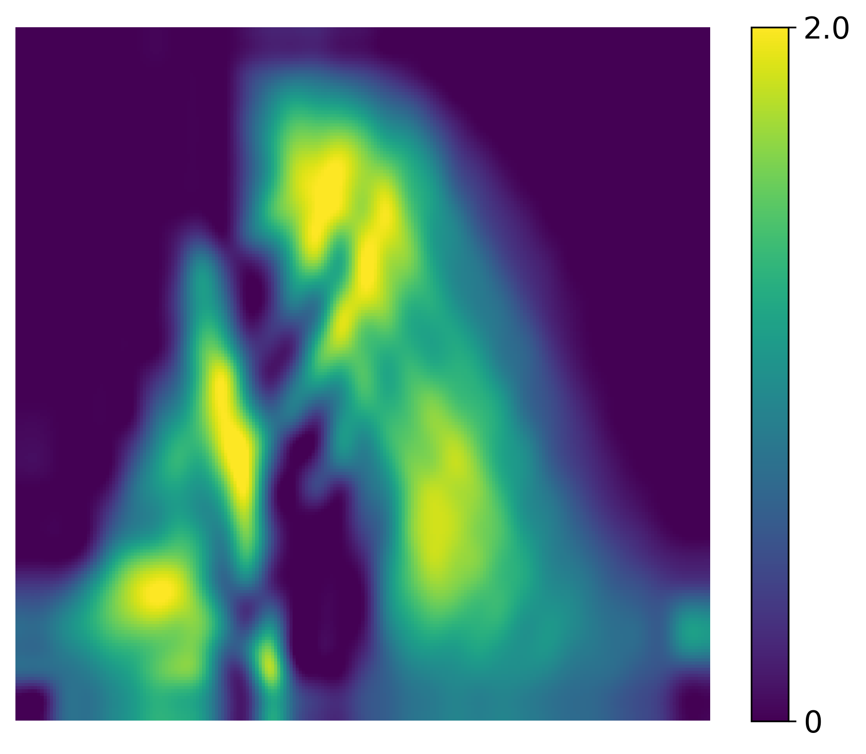
We investigate the impact of the temporal discretization by recovering an inclusion in the shape of the letter ‘$B$’, for which the true coefficient is $a(\mathbf{x})=2$, see (7.3) and (7.4). In this test, $\lambda=3$ in CWF (4.6), and the Tikhonov regularization parameter is set to $\alpha=3\times 10^{-5}$. We set the parameter $\varepsilon=0.01$ in (3.2), $c=5$ in (4.9) and the final time $T=4,$ as in (7.10). To simulate a realistic scenario, we add $1\%$ noise to the measurement data, i.e. $\sigma=0.01$ in (7.11), (7.12). We perform reconstructions for the CIP2 using three different numbers of time steps: $N_{t}\in\{10,20,40\}$. The results are displayed on Figure 2.

(a) True image

(b) $N_{t}=10$

(c) $N_{t}=20$

(d) $N_{t}=40$

Figure 2. Reconstruction results for different numbers of time steps $N_{t}=T/h=4/h,$ where $T=4$ as in (7.10), and $h$ is as in (3.15). Clearly, $N_{t}=20$ is the optimal number.

For $N_{t}=40$, the result is heavily contaminated by the numerical noise, rendering the image heavily corrupted by artifacts. For $N_{t}=10$, the reconstruction suffers from a significant blur. The clearest and the most accurate image is obtained with $N_{t}=20$. This finding highlights a counter-intuitive phenomenon of CIP2. Indeed, the idea that by decreasing the grid step size $h=4/N_{t}$ in (3.15) one would automatically improve the image quality does not work here. In fact, we demonstrate that the opposite is true for this ill-posed problem. Apparently, the step size $h$ in (3.15) acts as a sort of a regularization parameter here by filtering out high-frequency instabilities. Consequently, we fix $N_{t}=20$ for all subsequent numerical tests, which means $h=4/20=0.2.$

In Test 7.2 we numerically find the value of the optimal parameter $\varepsilon$ in (3.2).

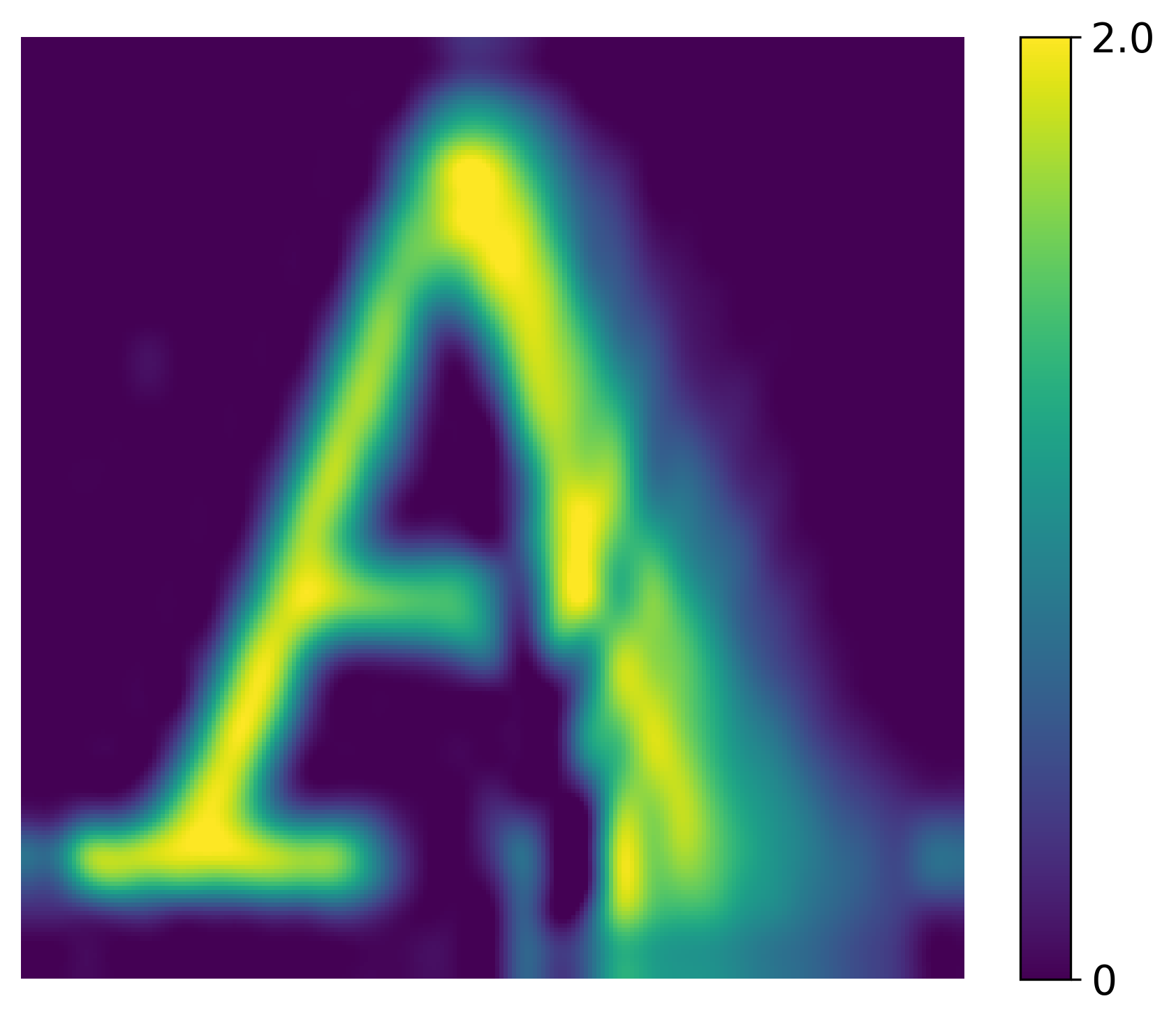
Test 7.2.

We now find an optimal value of the parameter $\varepsilon$ in (3.2). We test the case when the inclusion has the shape of the letter $\Omega$, for which the true coefficient $a(\mathbf{x})=2$ inside of this inclusion and $a(\mathbf{x})=0$ outside of it, see (7.3) and (7.4). In this test, $\lambda=3$ in CWF (4.6), the Tikhonov regularization parameter is $\alpha=3\times 10^{-5}$ and $N_{t}=20$. We again add 1% noise to the measurement data, i.e. $\sigma=0.01$ in (7.11), (7.12). The parameter $\varepsilon$ is varied over the set $\{0.001,0.01,0.03,0.05,0.1\}$, while the final time is fixed at $T=4$ as in (7.10) and $c=5$.

(a) True image

(b) $\varepsilon=0.001$

(c) $\varepsilon=0.01$

(d) $\varepsilon=0.03$

(e) $\varepsilon=0.05$

(f) $\varepsilon=0.1$

Figure 3. Reconstruction results illustrating the choice of an optimal value of the parameter $\varepsilon$ in (3.2). Obviously, $\varepsilon=0.01$ is the best one out of five values $\{0.001,0.01,0.03,0.05,0.1\}$. Hence, we assign the optimal value of this parameter $\varepsilon=0.01$ in all numerical tests below.

As observed in Figure 3, at $\varepsilon=0.001$, the reconstruction suffers from the numerical instability, resulting in significant distortions. Conversely, as $\varepsilon$ increases beyond $0.03$, the images become increasingly blurred due to the poor approximation in (3.2). At the same time, the value $\varepsilon=0.01$ yields both the sharpest and the most accurate reconstruction. Therefore, we set $\varepsilon=0.01$ for the subsequent tests.

In Test 7.3 we investigate the sensitivity of reconstruction results to the parameter $\lambda$ in the Carleman Weight Function $\varphi_{\lambda}\left(x_{1}\right)$ in (4.6).

Test 7.3.

We investigate the choice of the optimal value of the parameter $\lambda$ in CWF (4.6) by imaging an inclusion with the shape of the letter ’$A$’. The true coefficient $a(\mathbf{x})=2$ inside of this inclusion and $a(\mathbf{x})=0$ outside of it, see (7.3) and (7.4). Other parameters are set to the values determined from previous examples: $\varepsilon=0.01$, $T=4$, $N_{t}=20,$ $c=5$. To account for the data perturbations, 1% noise is added to the measurements, i.e. $\sigma=0.01$ in (7.11), (7.12). The Tikhonov regularization parameter is set to $\alpha=3\times 10^{-5}$, and reconstructions are performed for five values of the weight: $\lambda\in\{1,2,3,4,5\}$.

(a) True image

(b) $\lambda=1$

(c) $\lambda=2$

a

(d) $\lambda=3$

(e) $\lambda=4$

(f) $\lambda=5$

Figure 4. Reconstruction results illustrating the choice of an optimal value of the parameter $\lambda$ in Carleman Weight Function $\varphi_{\lambda}\left(x_{1}\right)$ in (4.6). Obviously, $\lambda=3$ is the best one out of five values $\{1,2,3,4,5\}$. Hence, we assign the optimal value of the parameter $\lambda=3$ in all numerical tests below.

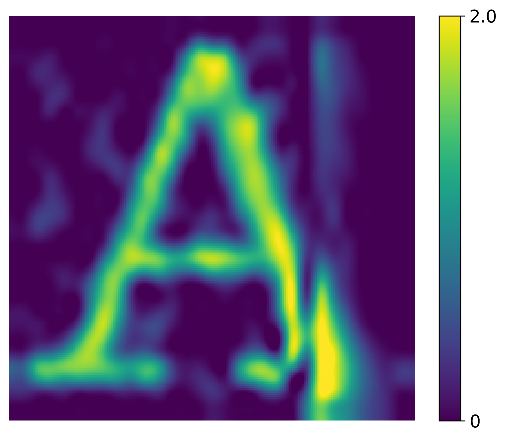
As shown in Figure 4, the reconstruction quality varies significantly with the value of $\lambda$. For smaller values ($\lambda=1,2$), the recovered images appear blurred, and the boundaries of the letter ‘$A$’ are poorly defined. In contrast, for larger values $\lambda=4,5$, the images exhibit noticeable artifacts and structural distortions; specifically, the limbs of the letter ‘$A$’ appear to be either disconnected or broken. The value $\lambda=3$ yields the clearest result, providing a sharp and continuous recovery of the inclusion shape with minimal background noise. Based on this observation, we fix $\lambda=3$ for the remainder of this study.

Based on Tests 7.1-7.3, we use the following values of the parameters in all tests below:

(7.14) $$T=4,\text{ }N_{t}=20,\text{ }\varepsilon=0.01,\text{ }\alpha=3\times 10^{-5},\text{ }\lambda=3,\text{ }c=5.$$

In the next two tests, we investigate the robustness of our method with respect to the different noise levels and coefficient values.

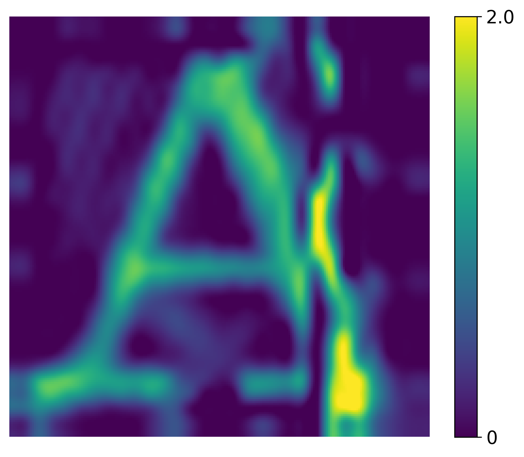
Test 7.4.

We investigate the impact of the noise level $\sigma$ in the boundary data (7.11), (7.12) via imaging an inclusion of the shape of the letters ’$SZ$’. The true coefficient is $a(\mathbf{x})=2$ inside of this inclusion and $a(\mathbf{x})=0$ outside of it, see see (7.3) and (7.4). The choice of parameters is as in (7.14). Noise levels of $1\%$, $3\%$, $5\%$ are added to the measurements, i.e. $\sigma=0.01,$ $0.03,$ $0.05$.

(a) True image

(b) 1% noise

(c) 3% noise

(d) 5% noise

Figure 5. Reconstruction results illustrating the sensitivity to the noise level. Even for the highest noise levels of 5% shapes of both inclusions are recognizable and the maximal value $\max a\left(\mathbf{x}\right)=2$ inside these letters is reconstructed accurately.

The reconstruction results are presented in Figure 5. As the noise level increases, we observe a corresponding increase in background artifacts and blurring. Nevertheless, even at the highest noise level of $5\%$, the geometry of the letters ‘$SZ$’ remains recognizable and the maximal value $\max a\left(\mathbf{x}\right)=2$ inside these letters is reconstructed accurately. This demonstrates a good degree of robustness of the method with respect to the random noise in the input data (7.11), (7.12).

Using (7.3) and (7.4), we now examine the influence of the magnitude $a$ of the value of the coefficient $a\left(\mathbf{x}\right)$ inside the inclusion on the quality of the reconstruction.

Test 7.5.

This test investigates the performance of our method for different values of the true coefficient $a(\mathbf{x})$. As in (7.3), we set the true coefficient to be constant within the inclusion and zero outside. The values of the constant $a$ within inclusions are taken as in (7.4), i.e. $a=2$, $3$, $5$,$10$. The shapes of inclusions are the letter ’$A$’ and the letters ’$SZ$’. All other parameters remain the same as the ones in (7.14). In all cases, $1\%$ noise is added to the measurements. The reconstructions are compared to assess the sensitivity of the method to the magnitude of the unknown coefficient.

(a) $a=2$

(b) $a=3$

(c) $a=5$

(d) $a=10$

(e) $a=2$

(f) $a=3$

(g) $a=5$

(h) $a=10$

Figure 6. Results of the reconstructions illustrating the sensitivity of our method to the value of the number $a$ in (7.3). Both shapes of inclusions and the maximal values of the unknown coefficient $a(\mathbf{x})$ are accurately reconstructed.

The results of the reconstructions are presented in Figure 6. The method successfully reconstructs the shapes of both inclusions for all tested coefficient values. Furthermore, the maximal values of the coefficient $a(\mathbf{x})$ are accurately reconstructed. It is noteworthy that the reconstruction quality does not degrade for larger values of $a(\mathbf{x})$. Even for the high value of $a=10$, the images remain sharp and accurate, confirming the capability of the convexification method to handle strongly nonlinear problems with large values of coefficients.

Finally, we present the results for the three-dimensional case.

Test 7.6.

We consider the reconstruction of 3-D inclusions of the shapes of the letters ‘$L$’ and ‘$K$’ located inside the unit cube $\Omega=[1,2]^{3}$. The true coefficient is $a(\mathbf{x})=2$ inside the inclusions and $a(\mathbf{x})=0$ elsewhere, see (7.3) and (7.4). The spatial domain is discretized using a $20\times 20\times 20$ grid. We set parameters as in (7.14). We add $1\%$ random noise to the boundary measurement data.

The reconstruction results are displayed in two separate figures for clarity. Figure 7 presents the 3-D isosurface plots of the reconstructed coefficient $a(\mathbf{x})$, illustrating the spatial recovery of the inclusions. Figure 8 provides the corresponding X-Z cross-sectional views (front view) to demonstrate the accuracy in the vertical plane, maintaining consistent color mapping between the 2-D cross-sections and 3-D isosurfaces.

(a) True 3-D image of ‘L’

(b) Reconstructed 3-D image of ‘L’

(c) True 3-D image of ‘K’

(d) Reconstructed 3-D image of ‘K’

Figure 7. Three-dimensional reconstruction results for different inclusion shapes (‘L’ and ‘K’). Here $a=2$, see (7.3).

(a) True ‘L’ in X-Z section

(b) Reconstructed ‘L’ in X-Z section

(c) True ‘K’ in X-Z section

(d) Reconstructed ‘K’ in X-Z section

Figure 8. Three-dimensional reconstruction results: X-Z cross-sectional views corresponding to Figure 7. Here $a=2$, see (7.3).

The reconstruction results are presented in Figures 7 and 8. As observed, the algorithm successfully reconstructs the spatial structures of both the ‘$L$’ and ‘$K$’ shapes with high fidelity. The value of the number $a$ inside the inclusions is also accurately reconstructed. The consistent accurate recoveries of these distinct 3-d geometries strongly validates the robustness of the proposed method.

8. Conclusions

For the first time, we have developed a globally convergent numerical method for the CIP posed in [8] in the most challenging case of the $\delta\left(\mathbf{x}\right)-$function in the initial condition for either the hyperbolic equation (2.6), (2.7) or the parabolic equation (2.16), (2.17). First, we have applied an analog of the Laplace transform to transform the original CIP for the wave equation with the unknown potential into a CIP for a similar parabolic equation. Next, we have developed a new approximate mathematical model for the latter CIP. This model is based on two approximations:

1. The approximation (3.2) of the solution of parabolic equation (2.16) with initial data (2.17). This approximation is based on the asymptotic behavior at $t\rightarrow 0^{+}$ of the fundamental solution of the parabolic equation (2.16), see (2.21)-(2.24) as established in Theorem 2.2.

2. The assumption of the representation via finite differences with condition (1.1) of the $t-$derivative of an associated integral differential equation (3.11).

We have developed a version of the globally convergent convexification numerical method for our approximate mathematical model. Global convergence here is understood in terms of Definition 1.1 of section 1. Furthermore, uniqueness theorem is proven for that model. This theorem partially addresses the original question of Gelfand, i.e. addresses that question within the framework of that model.

We have carried out exhaustive numerical studies of our method both in 2-d and 3-d cases. These studies revealed a high accuracy of our reconstructions of complicated structures for noisy data. We conclude, therefore, that this reconstruction accuracy confirms a high degree of the adequacy of our approximate mathematical model.

9. Appendix 1: Proof of Theorem 2.1

We use here the decomposition of the fundamental solution of problem (2.6), (2.7), which is given in [31, Lemmata 2.2.1 and 2.2.3]. In this book the representation of the solution is in the form of infinite series, assuming that coefficients of the corresponding hyperbolic equation belong $C^{\infty}(\mathbb{R}^{n})$. Unlike this, we assume here that the coefficient $a(\mathbf{x})\in C^{l}\left(\mathbb{R}^{n}\right),$ $\ell=5[n/2]+3,$ see (2.4). Hence, we use only a finite segment of this series with a remainder term. This representation of the solution is given below for odd and even $n$ separately.

We start with the representation (2.9) for $n=2m+1$, $m\geq 1$. In this case formulae (2.10) for functions $\alpha_{k}(\mathbf{x})$ are given in [31, page 32]. It follows from formulae (2.10) that $\alpha_{s}\in C^{\ell-2(s+m)}(\mathbb{R}^{n})$, $s=\left[-m,S\right],$ and all $\alpha_{k}(\mathbf{x})$ are bounded in $\mathbb{R}^{n}$, since

$$\ell=5\left[\frac{n}{2}\right]+3>2(S+m)=2\left(2m+1\right)=2n+2.$$

Substituting representation (2.9) in equation (2.6) and takin into account that $\alpha_{k}(\mathbf{x})$ are solutions of equations

$$\left.\begin{array}[]{c}2\nabla\alpha_{-m}(\mathbf{x})\cdot\nabla\left(|\mathbf{x}|^{2}\right)=0,\\ 2\nabla\alpha_{s}(\mathbf{x})\cdot\nabla\left(|\mathbf{x}|^{2}\right)+4(s-m)\alpha_{s}(\mathbf{x})=\Delta\alpha_{s-1}(\mathbf{x})+a(\mathbf{x})\alpha_{s-1}(\mathbf{x}),~s\in\left[-m+1,S\right],\end{array}\right.$$

we obtain that the function ${v}_{S}(\mathbf{x},t)$ is the solution of the following problem

(9.1) $$\left.\begin{array}[]{c}2\left(\partial_{t}^{2}-\Delta-a(\mathbf{x})\right){v}_{S}=h_{S}(\mathbf{\ x},t),~\mathbf{x}\in\mathbb{R}^{n},~t>|\mathbf{x}|,\\ {v}_{S}(\mathbf{x},t)|_{t<|\mathbf{x}|}=0,\end{array}\right.$$

where

$$h_{S}(\mathbf{x},t)=\left(\Delta\alpha_{S}(\mathbf{x})+a(\mathbf{x})\alpha_{S}(\mathbf{x})\right)\theta_{S}(t^{2}-|\mathbf{x}|^{2}).$$

The equality ${v}_{S}(\mathbf{x},t)=0$ for $t<|\mathbf{x}|$ follows from the fact that the speed of sound is $1$.

Below $B_{1},B_{2}>0$ denote different numbers depending only on the number $a_{0}$ in (2.4). Let $D_{t}=\{(\mathbf{x},\tau):\mathbf{x}\in\mathbb{\ R}^{n},0<\tau\leq t\}$. The function $h_{S}\in H^{S}(D_{t})$ since $\ell=2(S+m+1)+S$. Using the method of energy estimates method and condition (2.4), one can prove the following estimate

(9.2) $$\|{v}_{S}\|_{H^{S+1}(\Omega_{t})}\leq B_{1}e^{B_{2}t}\|h_{S}\|_{H^{S}(D_{t})},~\forall t>0,$$

where the domain $\Omega_{t}$ is defined in (2.8), and numbers $C_{1}$ and $C_{2}$ depend only on $a_{0}$. Since

(9.3) $$\|h_{S}\|_{H^{S}(D_{t})}\leq B_{1}t^{\eta_{S}},$$

where $\eta_{S}=S+n+1$, then the following estimate holds

(9.4) $$\|{v}_{S}\|_{H^{S+1}(\Omega_{t})}\leq B_{1}t^{\eta_{S}}e^{B_{2}t}\|h_{S}\|_{H^{S}(D_{t})},~\forall t>0.$$

Since $2(S+1)>n+2$ then by the Sobolev embedding theorems, ${v}_{S}\in C^{2}(\Omega_{t})$. Hence, using (9.3) and (9.4), we obtain

(9.5) $$\|{v}_{S}\|_{C^{2}(\Omega_{t})}\leq B_{1}e^{B_{2}t},~\forall t>0.$$

Equation (9.1) and inequality (9.5) imply

(9.6) $$\|\partial_{t}^{2}{v}_{S}\|_{C(\Omega_{t})}\leq B_{1}e^{B_{2}t},~\forall t>0,$$

which implies

(9.7) $$\|\partial_{t}{v}_{S}\|_{C(\Omega_{t})}\leq B_{1}e^{B_{2}t},~\forall t>0.$$

Hence, we have proved that the function ${v}_{S}(\mathbf{x},t)$ is bounded in the domain $\Omega_{t}$ together with its derivatives up to the second order for any fixed $t>0$. In addition, we have proven that this function grows not faster than $e^{B_{2}t}$ as $t\rightarrow\infty$, together with its derivatives up to the second order.

Consider now the case $n=2m,m\geq 1$. In this case the representation of the solution of problem (2.6), (2.7) has the form (2.11), where the function ${v}_{S}(\mathbf{x},t)$ is the solution of the Cauchy problem (9.1) with $h_{S}(\mathbf{x},t)$ given by

$$h_{S}(\mathbf{x},t)=\left(\Delta\alpha_{S}(\mathbf{x})+a(\mathbf{x})\alpha_{S}(\mathbf{x})\right)\theta_{S+1/2}(t^{2}-|\mathbf{x}|^{2}).$$

Since $S=m+1$, then estimates (9.2)-(9.7) are also valid for the function ${v}_{S}(\mathbf{x},t)$ with $\eta_{S}=S+n+3/2$. In addition, the following estimates are valid:

(9.8) $$\left.\begin{array}[]{c}\|v_{S}(\mathbf{x},t)\|_{C^{2}(B_{R})}\leq B_{1}e^{B_{2}t},~t>0,\\ \|\partial_{t}v_{S}(\mathbf{x},t)\|_{C^{2}(B_{R})}\leq B_{1}e^{B_{2}t},~t>0,\\ \|\partial_{t}^{2}v_{S}(\mathbf{x},t)\|_{C^{2}(B_{R})}\leq B_{1}e^{B_{2}t},~t>0.\end{array}\right.$$

$\square$

10. Appendix 2: Proof of Theorem 2.2

By (2.1) $a\left(\mathbf{x}\right)=0$ in a small neighborhood of the point $\left\{\mathbf{x}=0\right\}.$ Hence, uniqueness and existence of the solution $u\left(\mathbf{x},t\right)$ of problem (2.16), (2.17) satisfying (2.20) easily follow from results of Chapter 4 of [23]. Theorem 2.1 guarantees the existence of transformation (2.14) for the function $U$ and its derivatives up to the second order. More precisely,

$$u\left(\mathbf{x},t\right)=\mathcal{L}\left(U\right),u_{x_{i}}\left(\mathbf{x},t\right)=\mathcal{L}\left(U_{x_{i}}\right),\text{ }u_{x_{i}x_{j}}\left(\mathbf{x},t\right)=\mathcal{L}\left(U_{x_{i}x_{j}}\right),\text{ }u_{t}\left(\mathbf{x},t\right)=\mathcal{L}\left(U_{tt}\right).$$

We need to prove asymptotic formulae (2.21)-(2.24).

Let $n=2m+1$. Substituting representation (2.9) in (2.14) and using (2.13), we obtain

$$u(\mathbf{x},t)=\frac{e^{-\frac{|\mathbf{x}|^{2}}{4t}}}{4\sqrt{\pi t^{3}}}\int\limits_{0}^{\infty}\left[\sum\limits_{s=-m}^{S}\alpha_{s}(\mathbf{x})\theta_{s}(z)+{v}_{S}(\mathbf{x},\sqrt{z+|\mathbf{x}|^{2}})\right]e^{-\frac{z}{4t}}dz.$$

where $S=m+1,$ and estimates (9.5)-(9.7) hold for the function ${v}_{S}(\mathbf{x},t)$. Simple calculations lead to the formula

(10.1) $$u(\mathbf{x},t)=\frac{e^{-\frac{|\mathbf{x}|^{2}}{4t}}}{4\sqrt{\pi t^{3}}}\left[w_{S}(\mathbf{x},t)+\overline{w}_{S}(\mathbf{x},t)\right],\quad t>0,$$

where

(10.2) $$w_{S}(\mathbf{x},t)=\sum\limits_{s=-m}^{S}\alpha_{s}(\mathbf{x})(4t)^{s+1},$$

(10.3) $$\overline{w}_{S}(\mathbf{x},t)=\int\limits_{0}^{\infty}e^{-\frac{z}{4t}}{v}_{S}\left(\mathbf{x},\sqrt{z+|\mathbf{x}|^{2}}\right)\,dz.$$

Using estimates (9.5)-(9.7), we obtain

(10.4) $$\left.\begin{array}[]{c}\overline{w}_{S}(\mathbf{x},t)=O(t),\\ \partial_{x_{i}}\overline{w}_{S}(\mathbf{x},t)=O(t),~i\in\left[1,n\right],\\ \partial_{x_{i}x_{j}}\overline{w}_{S}(\mathbf{x},t)=O(t),~i,j\in\left[1,n\right],\\ \partial_{t}\overline{w}_{S}(\mathbf{x},t)=O(t),\\ \mathbf{x}\in B_{M},\text{ }t\rightarrow 0^{+},\end{array}\right.$$

for any fixed $M>0$. Indeed, to prove the formula in the first line of (10.4), we use (9.5). Hence,

$$\left|\overline{w}_{S}(\mathbf{x},t)\right|\leq\int\limits_{0}^{\infty}e^{-\frac{z}{4t}}\left|{v}_{S}\left(\mathbf{x},\sqrt{z+|\mathbf{x}|^{2}}\right)\right|\,dz\leq B_{1}\int\limits_{0}^{\infty}e^{-\frac{z}{4t}}e^{B_{2}\sqrt{z+|\mathbf{x}|^{2}}}\,dz\leq$$

(10.5) $$\leq 4tB_{1}e^{B_{2}M}\int\limits_{0}^{\infty}e^{-y+2B_{2}\sqrt{ty}}\,dy=O(t),~\mathbf{x}\in B_{M},~t\rightarrow 0^{+}.$$

Estimates in the second and third lines of (10.4) of the first and second derivatives of the function $\overline{w}_{S}(\mathbf{x},t)$ with respect to $x_{i}$ can be done similarly. However the estimate of the derivative of the function $\overline{w}_{S}(\mathbf{x},t)$ with respect to $t$ in the fourth line of (10.4) requires more explanations.

First, we note that

(10.6) $$\int\limits_{0}^{\infty}e^{-\frac{s}{4t}}{v}_{S}\left(\mathbf{x},\sqrt{z+|\mathbf{x}|^{2}}\right)\,dz=(4t)^{2}\int\limits_{0}^{\infty}e^{-\frac{z}{4t}}\partial_{z}^{2}\left[v_{S}\left(\mathbf{x},\sqrt{z+|\mathbf{x}|^{2}}\right)\right]\,dz.$$

Hence,

$$\partial_{t}\int\limits_{0}^{\infty}e^{-\frac{z}{4t}}{v}_{S}\left(\mathbf{\ x},\sqrt{z+|\mathbf{x}|^{2}}\right)\,dz=4\int\limits_{0}^{\infty}z\,e^{-\frac{s}{4t}}\partial_{z}^{2}\left[v_{S}\left(\mathbf{x},\sqrt{z+|\mathbf{\ x}|^{2}}\right)\right]\,dz.$$

Hence, using (9.6) and (10.5), we obtain

$$\left|\partial_{t}\int\limits_{0}^{\infty}e^{-\frac{z}{4t}}{v}_{S}\left(\mathbf{x},\sqrt{z+|\mathbf{x}|^{2}}\right)\,dz\right|\leq 4\int\limits_{0}^{\infty}z\,e^{-\frac{s}{4t}}\left|\partial_{z}^{2}\left[v_{S}\left(\mathbf{x},\sqrt{z+|\mathbf{x}|^{2}}\right)\right]\right|\,dz\leq$$

$$\leq B_{1}\int\limits_{0}^{\infty}\,e^{-\frac{s}{4t}}ze^{B_{2}\sqrt{z+|\mathbf{x}|^{2}}}dz=O\left(t\right),~\mathbf{x}\in B_{M},~t\rightarrow 0^{+},$$

which proves the estimate in the fourth line of (10.4).

We now work with the function $w_{S}(\mathbf{x},t)$ in (10.1), (10.2). First, we note that by (2.10)

$$\frac{e^{-\frac{|\mathbf{x}|^{2}}{4t}}}{4\sqrt{\pi t^{3}}}\alpha_{-m}(\mathbf{x})(4t)^{1-m}=\frac{1}{(2\sqrt{\pi t})^{n}}\,e^{-\frac{|\mathbf{x}|^{2}}{4t}}=u_{0}(\mathbf{x},t).$$

Hence, we can rewrite representation (10.1) in the form

(10.7) $$u(\mathbf{x},t)=u_{0}(\mathbf{x},t)\left[\widehat{w}_{S}(\mathbf{x},t)+2\pi^{m}(4t)^{m-1}\overline{w}_{S}(\mathbf{x},t)\right],\quad t>0,$$

where

(10.8) $$\begin{array}[]{l}\widehat{w}_{S}(\mathbf{x},t)=1+\sum\limits_{s=-m+1}^{S}\widehat{\alpha}_{s}(\mathbf{x})(4t)^{s+m},\\ \widehat{\alpha}_{s}(\mathbf{x})=\frac{1}{4}\int\limits_{0}^{1}z^{s+m-1}(\Delta\alpha_{s-1}(\xi)+a(\xi)\alpha_{s-1}(\xi))|_{\xi=z\mathbf{x}}\,dz,~\>s\in\left[-m+1,S\right].\end{array}$$

Representation (2.21) with $\kappa=1$ follows from (10.7) and (10.8). Differentiating (10.7) with respect to $t$ and using (10.4) , we obtain

$$u_{t}(\mathbf{x},t)=\partial_{t}u_{0}(\mathbf{x},t)[1+O(t)]+$$

$$+u_{0}(\mathbf{x},t)\left[O(t)+2\pi^{m}\partial_{t}\left((4t)^{m-1}\int\limits_{0}^{\infty}e^{-\frac{z}{4t}}{v}_{S}\left(\mathbf{x},\sqrt{z+|\mathbf{x}|^{2}}\right)\,dz\right)\right],~\mathbf{x}\in B_{M},\text{ }t\rightarrow 0.$$

Using (10.6), we obtain

$$\partial_{t}\left((4t)^{m-1}\int\limits_{0}^{\infty}e^{-\frac{z}{4t}}{v}_{S}\left(\mathbf{x},\sqrt{z+|\mathbf{x}|^{2}}\right)\,dz\right)=$$

$$\qquad=4(m+1)(4t)^{m}\int\limits_{0}^{\infty}e^{-\frac{z}{4t}}\partial_{z}^{2}\left[v_{S}\left(\mathbf{x},\sqrt{z+|\mathbf{x}|^{2}}\right)\right]\,dz=$$

$$\qquad+4(4t)^{m-1}\int\limits_{0}^{\infty}z\,e^{-\frac{z}{4t}}\partial_{z}^{2}\left[v_{S}\left(\mathbf{x},\sqrt{z+|\mathbf{x}|^{2}}\right)\right]\,dz=O(t^{m}),~\mathbf{x}\in B_{M},~t\rightarrow 0^{+}.$$

Hence,

$$u_{t}(\mathbf{x},t)=\partial_{t}u_{0}(\mathbf{x},t)[1+O(t)],~\mathbf{x}\in B_{M},~t\rightarrow 0^{=}.$$

It proves relation (2.22) with $\kappa=1$.

Differentiating (10.7) with respect to $x_{i}$ and using again (10.4), we obtain

$$u_{x_{i}}(\mathbf{x},t)=\partial_{x_{i}}u_{0}(\mathbf{x},t)[1+O(t)]+u_{0}(\mathbf{x},t)\,O(t),~t\rightarrow 0^{+}.$$

Also,

$$u_{0}(\mathbf{x},t) = -\partial_{x_{i}}u_{0}(\mathbf{x},t)\frac{2t}{x_{i}}=$$

$$= \partial_{x_{i}}u_{0}(\mathbf{x},t)\,O(t),~\mathbf{x}\in G_{\sigma}(M),~t\rightarrow 0^{+}.$$

Hence,

$$u_{x_{i}}(\mathbf{x},t)=\partial_{x_{i}}u_{0}(\mathbf{x},t)[1+O(t)],~\mathbf{x}\in G_{\sigma}(M),~t\rightarrow 0^{+}.$$

The latter equality is the same as the one in (2.23) with $\kappa=1$. The proof of equality (2.24) with $\kappa=1$ is similar.

Thus, Theorem 2.2 is proven for the case when $n=2m+1,m\geq 1$, $\ell=5m+3=5[n/2]+3$.

Consider now case $n=2m,$ $m\geq 1$. Then (2.13) and (2.14) lead to

$$u(\mathbf{x},t)=\frac{e^{-\frac{|\mathbf{x}|^{2}}{4t}}}{4\sqrt{\pi t^{3}}}\int\limits_{0}^{\infty}e^{-\frac{s}{4t}}\left[\sum\limits_{s=-m}^{S}\alpha_{s}(\mathbf{x})\theta_{s+1/2}(z)+{v}_{S}\left(\mathbf{x},\sqrt{z+|\mathbf{x}|^{2}}\right)\right]dz.$$

This equality can be represented in the form similar to (10.1):

(10.9) $$u(\mathbf{x},t)=\frac{e^{-\frac{|\mathbf{x}|^{2}}{4t}}}{4\sqrt{\pi t^{3}}}\left[2\sqrt{\pi t}\,w_{S}(\mathbf{x},t)+\overline{w}_{S}(\mathbf{x},t)\right],\quad t>0,$$

where functions $w_{S}(\mathbf{x},t)$ and $\overline{w}_{S}(\mathbf{x},t)$ are determined by formulae (10.2) and (10.3), respectively.

If $S=m+1$ then estimates (9.2)-(9.7) are also valid for ${v}_{S}(\mathbf{x},t)$ with $\eta_{S}=S+n+3/2,$ and estimates (9.8) hold as well.

Note that in this case

$$\frac{e^{-\frac{|\mathbf{x}|^{2}}{4t}}}{4\sqrt{\pi t^{3}}}\,\left(2\sqrt{\pi t}\right)\alpha_{-m}(4t)^{1-m}=\frac{e^{-\frac{|\mathbf{x}|^{2}}{4t}}}{(4{\pi t})^{n/2}}=u_{0}(\mathbf{x},t).$$

Hence, representation (10.9) we can be written as:

(10.10) $$u(\mathbf{x},t)=u_{0}(\mathbf{x},t)\left[\widehat{w}_{K}(\mathbf{x},t)+\pi^{m-1/2}(4t)^{m-3/2}\bar{w}_{K}(\mathbf{x},t)\right],\quad t>0,$$

where $\widehat{w}_{K}(\mathbf{x},t)$ is given by the first line of (10.8). Note that representation (10.10) differs from representation (10.7) by the term $(4t)^{m-3/2}$, where the power $m-3/2$ is less by $1/2,$ as compares with ${m-1}$ in (10.7). It is important if $m=1,$ then $n=2.$ only. If $m>1$, then the validity of Theorem 2.2 with $\kappa=1$ follows from representation (10.10) and inequalities (9.2)-(9.7), (9.8) just as it was in the above case when $n$ is odd. However, if $n=2,$ then $m=1$, and we need to put $\kappa=1/2$ in estimates (2.21)-(2.24) .

Thus, Theorem 2.2 is proven in both cases: odd and even $n$. $\square$

References

- [1] A. B. Bakushinskii, M. V. Klibanov, and N. A. Koshev, Carleman weight functions for a globally convergent numerical method for ill-posed Cauchy problems for some quasilinear PDEs, Nonlinear Anal. Real World Appl. 34 (2017), 201–224. doi:10.1016/j.nonrwa.2016.08.008
- [2] L. Beilina, Domain decomposition finite element/finite difference method for the conductivity reconstruction in a hyperbolic equation, Commun. Nonlinear Sci. Numer. Simul. 37 (2016), 222–237. doi:10.1016/j.cnsns.2016.01.016
- [3] L. Beilina and E. Lindström, An adaptive finite element/finite difference domain decomposition method for applications in microwave imaging, Electronics 11 (2022), 2079-9292. doi:10.3390/electronics11091359
- [4] Yu. M. Berezanski, The uniqueness theorem in the inverse problem of spectral analysis for the Schrödinger equation, Trudy Moskov. Mat. Obšč. 7 (1958), 1–62.
- [5] M. Boulakia, M. de Buhan, T. Delaunay, S. Imperiale and P. Moireau, Solving inverse source wave problem—from Carleman estimates to observer design, Math. Control Relat. Fields 16 (2026), 40–81. doi:10.3934/mcrf.2025007
- [6] A. L. Bukhgeim and M. V. Klibanov, Global uniqueness of a class of multidimensional inverse problems, Soviet Mathematics Doklady, 24 (1981), 244-247.
- [7] G. Chavent, Nonlinear Least Squares for Inverse Problems: Theoretical Foundations and Step-by-Step Guide for Applications, Springer, Dordrecht, 2009. doi:10.1007/978-90-481-2785-6
- [8] I. M. Gelfand, Some problems of functional analysis and algebra, Proceedings of the International Congress of Mathematicians (Amsterdam, 1954), Vol. 1, North-Holland, Amsterdam, 1957, pp. 253–276.
- [9] A. V. Goncharsky and S. Y. Romanov, Iterative methods for solving coefficient inverse problems of wave tomography in models with attenuationn, Inverse Probl. 33 (2017), 025003. doi:10.1088/1361-6420/33/2/025003
- [10] A. V. Goncharsky, S. Y. Romanov, and S. Y. Seryozhnikov, On mathematical problems of two-coefficient inverse problems of ultrasonic tomography, Inverse Probl. 40 (2024), 045026. doi:10.1088/1361-6420/ad2aa9
- [11] V. Isakov, Inverse Problems for Partial Differential Equations, 3rd ed., Springer, Cham, 2017. doi:10.1007/978-3-319-51658-5
- [12] M. V. Klibanov, Inverse problems and Carleman estimates, Inverse Probl. 8 (1992), 575–596. doi:10.1088/0266-5611/8/4/009
- [13] M.V. Klibanov and O.V. Ioussoupova, Uniform strict convexity of a cost functional for three dimensional inverse scattering problem, SIAM J. Math. Anal. 26 (1995), 147–179. doi:10.1137/S0036141093244039
- [14] M. V. Klibanov, Global convexity in a three-dimensional inverse acoustic problem, SIAM J. Math. Anal. 28 (1997), 1371–1388. doi:10.1137/S0036141096297364
- [15] M. V. Klibanov and T. R. Lucas and R. M. Frank, A fast and accurate imaging algorithm in optical/diffusion tomography, Inverse Problems 13 (1997), 1341–1361. doi:10.1088/0266-5611/13/5/015
- [16] M.V. Klibanov, Carleman estimates for global uniqueness, stability and numerical methods for coefficient inverse problems, J. Inverse Ill-Posed Probl. 21 (2013), 477–560. doi:10.1515/jip-2012-0072.
- [17] M.V. Klibanov, J. Li and W. Zhang, Convexification for an inverse parabolic problem, Inverse Probl. 36 (2020), 085008. doi:10.1088/1361-6420/ab9893
- [18] M.V. Klibanov and J. Li, Inverse Problems and Carleman Estimates: Global Uniqueness, Global Convergence and Experimental Data, De Gruyter, Berlin, 2021. doi:10.1515/9783110745481
- [19] M. V. Klibanov, V. A. Khoa, A. V. Smirnov, Loc H. Nguyen, G. W. Bidney, Lam H. Nguyen, A. Sullivan, and V. N. Astratov, Convexification inversion method for nonlinear SAR imaging with experimentally collected data, J. Appl. Ind. Math. 15 (2021), 413–436. doi:10.1134/s1990478921030054
- [20] M.V. Klibanov, A new type of ill-posed and inverse problems for parabolic equations, Commun. Anal. Comput. 2 (2024), 367–398. doi:10.3934/cac.2024018
- [21] M.V. Klibanov, J. Li and Z. Yang, Convexification numerical method for a coefficient inverse problem for the system of nonlinear parabolic equations governing mean field games, Inverse Probl. Imaging 19 (2025), 219–252. doi:10.3934/ipi.2024031
- [22] M. V. Klibanov and J. Li, Carleman Estimates in Mean Field Games, De Gruyter, Berlin, 2025. doi:10.1515/9783111723112
- [23] O. A. Ladyzhenskaya, V. A. Solonnikov, and N. N. Uralceva, Linear and Quasilinear Equations of Parabolic Type, American Mathematical Society, Providence, RI, 1968.
- [24] M.M. Lavrent’ev, V.G. Romanov and S.P. Shishatskii, Ill-Posed Problems of Mathematical Physics and Analysis, American Mathematical Society, Providence, RI, 1986.
- [25] S. Ma and M. Salo, Fixed angle inverse scattering in the presence of a Riemannian metric, J. Inverse Ill-Posed Probl. 30 (2022), 495–520. doi:10.1515/jiip-2020-0119
- [26] V. A. Marchenko, Certain problems in the theory of second-order differential operators, Doklady Akad. Nauk SSSR 72 (1950), 457-463.
- [27] V. A. Marchenko, Sturm-Liouville operators and applications, Revised, AMS Chelsea Publishing, Providence, RI, 1986. doi:10.1090/chel/373
- [28] R. G. Novikov, The approach to approximate inverse scattering at fixed energy in three dimensions, IMRP Int. Math. Res. Pap. 6 (2005), 287–349. doi:10.1155/IMRP.2005.287
- [29] Rakesh and M. Salo, The fixed angle scattering problem and wave equation inverse problems with two measurements, Inverse Probl. 36 (2020), 035005. doi:10.1088/1361-6420/ab23a2
- [30] Rakesh and M. Salo, Fixed angle inverse scattering for almost symmetric or controlled perturbations, SIAM J. Math. Anal. 52 (2020), 5467–5499. doi:10.1137/20M1319309
- [31] V.G. Romanov, Investigation Methods for Inverse Problems, VSP, Utrecht, 2002. doi:10.1515/9783110943849
- [32] V.G. Romanov, Ray statement of the acoustic tomography problem, Dokl. Math. 106 (2022), 254–258. doi:10.1134/S1064562422040147
- [33] J.A. Scales, M.L. Smith, T.L. Fisher, Global optimization methods for multimodal inverse problems, J. Comput. Phys. 103 (1992), 258-268. doi:10.1016/0021-9991(92)90400-S
- [34] A.N. Tikhonov, A.V. Goncharsky, V.V. Stepanov and A.G. Yagola, Numerical Methods for the Solution of Ill-Posed Problems, Kluwer Academic Publishers Group, Dordrecht, 1995. doi:10.1007/978-94-015-8480-7
- [35] B.R. Vainberg, Asymptotic methods in equations of mathematical physics, CRC Press, London, 1989. doi:10.1201/9781003580423