Time-varying System Identification of Bedform Dynamics Using Modal Decomposition

Abstract

Measuring sediment transport in riverbeds has long been a challenging research problem in geomorphology and river engineering. Traditional approaches rely on direct measurements using sediment samplers. Although such measurements are often considered ground truth, they are intrusive, labor-intensive, and prone to large variability. As an alternative, sediment flux can be inferred indirectly from the kinematics of migrating bedforms and temporal changes in bathymetry. While such approaches are helpful, bedform dynamics are nonlinear and multiscale, making it difficult to determine the contributions of different scales to the overall sediment flux. Fourier decomposition has been applied to examine bedform scaling, but it treats spatial and temporal variability separately. In this work, we introduce Dynamic Mode Decomposition (DMD) as a data-driven framework for analyzing riverbed evolution. By incorporating this representation into the Exner equation, we establish a link between modal dynamics and net sediment flux. This formulation provides a surrogate measure for scale-dependent sediment transport, enabling new insights into multiscale bedform-driven sediment flux in fluvial channels.

I Introduction

Accurately modeling and predicting sediment transport in fluvial environments remains a fundamental challenge in geomorphology and river engineering. Fluvial channels act as primary conduits for both water and sediment [9, 8]. The continuous processes of erosion and deposition shape Earth’s surface, influence ecological diversity, and affect human activities such as navigation, flood control, and infrastructure development [21]. Since sediment transport underpins both the morphology and function of channel systems, reliable approaches for its quantification are of critical importance.

Traditionally, sediment transport has been measured directly using devices such as sediment traps or Helley–Smith samplers, which capture material moving along the bed over a specified interval [20, 4, 17, 1]. While often regarded as ground truth, these methods are labor-intensive, intrusive, and highly sensitive to deployment conditions. Reported measurements vary substantially in space and time, in addition to factors such as sampler orientation, mesh size, sediment grain distribution, and the hydrodynamic disturbance created by the device itself. As a result, direct sampling is not only time-consuming but also limited in accuracy and duration, making it insufficient for resolving the dynamics of sediment flux in natural channels. Given these limitations, researchers have increasingly turned to indirect approaches. One widely adopted method is to infer sediment flux from the kinematics of migrating bedforms and from temporal changes in channel bathymetry (see for details [18, 9, 19]). Bedforms act as signatures of sediment motion. Their characteristics, such as amplitude, wavelength, and migration velocity, can provide indirect estimates of volumetric sediment flux [16]. The volumetric sediment flux, $q_{s}$, represents the rate at which sediment volume passes per unit channel width. Estimating $q_{s}$ is central to quantifying bedload transport. However, bedform dynamics are inherently nonlinear and strongly scale dependent [14]. Bedforms of different sizes coexist, migrate at distinct velocities, and interact through feedbacks among morphology, shear stress, and transport rate [9, 19, 2]. This multiscale variability makes it difficult to determine the relative contributions of different bedform scales to the overall sediment flux, which remains an open research question. Previous studies have used Fourier decomposition of bed elevation fields to examine scaling behavior and the role of different bedform sizes in sediment transport [3]. These analyses showed that small, fast-migrating secondary bedforms can significantly contribute to flux and drive the propagation of larger, slower bedforms. While Fourier methods provide valuable spectral information, they treat spatial and temporal variations separately.

Figure 1: Riverbed topography visualization. (a) Illustrates 2D topography at a specific time. (b) Spatial bed elevation profile along a selected transect (shown in red line in Figure 1(a)). (c) Spatio-temporal evolution of the riverbed topography. The figure also describes the dimensions of the data. (d) Temporal bed elevation profile along a selected point.

Dynamic Mode Decomposition (DMD) has emerged as a widely used tool in fluid mechanics and data-driven modeling, valued for its ability to extract coherent spatio-temporal patterns and provide reduced-order representations of complex flow fields [5, 15, 10]. In this work, we propose a novel framework based on DMD for characterizing the scale dependence of sediment transport analysis. DMD decomposes the evolution of bed elevation into spatio-temporal modes, each representing a coherent pattern with an associated growth/decay rate and frequency. This makes DMD particularly well-suited for the “tall-and-skinny” structure of riverbed elevation datasets, where many spatial samples are collected over relatively short time records [7]. By substituting the DMD-based linear approximation of bed elevation dynamics into the Exner equation and integrating across space, we establish a connection between DMD modes and net sediment flux.

Contributions: The contributions of this article are as follows:

• The paper studies the spatio-temporal coherent structure of the riverbed elevation using DMD.

• It derives a mathematical connection between sediment flux and spatio-temporal modes of riverbed elevation computed from DMD.

II Data Description

The dataset analyzed in this study originates from large-scale flume experiments conducted at the St. Anthony Falls Laboratory (SAFL) Main Channel. The flume is $85\,m$ long and horizontally $2.75\,m$ wide and is equipped with discharge regulation and sediment recirculation systems to maintain morphodynamic equilibrium during experiments [8]. The spatio-temporal bed evolution was measured along the channel centerline using a submerged laser scanning device mounted on an automated cart. The dataset consists of three-dimensional arrays of bed elevation change, denoted as $\eta(x,y,t)$, where $t$ represents the acquisition time in seconds, $x$ the streamwise locations, and $y$ the spanwise locations. Formally, $\eta(x,y,t)\in\mathbb{R}^{N_{x}\times N_{y}\times N_{t}},$ where $N_{x}$, $N_{y}$, and $N_{t}$ correspond to the number of streamwise, spanwise, and temporal indices, respectively. Figure 1 explains the bed elevation data. Figure 1 (a) illustrates the topography at a given moment. In the stream direction, the bed is $12\;m$ long and $0.5\;m$ wide. The elevation of the bed is limited between $0$ to $0.329\;m$. There are $3008$ points in the stream direction $(N_{x}=3008)$ and there are $126$ points in the span direction ($N_{y}=126$). Figure 1 (b) shows the elevation of the river bed along a transect. Figure 1(c) shows the temporal evolution of the topography by representing the three-dimensional bed elevation in Figure 1(a) as a two-dimensional heat map, which also illustrates the dimensions of the spatio-temporal data. Figure 1 (d) shows the temporal evolution of a point at the middle of the channel on a transect. The data was recorded for $9.71$ hours at a resolution of approximately $2\;\text{min}$, which corresponds to $300$ time snapshots. This high-resolution spatio-temporal record of channel bed morphology provides an ideal basis for applying dynamic mode decomposition (DMD) to investigate the coherent structures and temporal dynamics of riverbed evolution.

III DMD Framework for Bed Elevation

III-A Formulation of DMD for Bed-Elevation Fields

DMD is a data-driven technique that extracts coherent spatio-temporal patterns from data by decomposing it into modes and complex eigenvalues. Each mode represents a spatial structure, while each eigenvalue characterizes the temporal behavior through a growth/decay rate and oscillation frequency [7]. In practice, DMD assumes that consecutive snapshots of the system satisfy an approximate linear evolution of the form $X^{\prime}=AX$. Here, $X=[x_{1},x_{2},\ldots,x_{m-1}]$ and $X^{\prime}=[x_{2},x_{3},\ldots,x_{m}]$ are snapshot matrices constructed from sequential measurements of the system state, where each column $x_{k}$ represents a vectorized snapshot of the spatial field at time $t_{k}$. The operator $A$ is an unknown linear mapping that advances the state from one snapshot to the next. DMD estimates this operator directly from data and computes its eigenvalues and eigenvectors to obtain the dominant dynamical modes. This procedure yields a reduced-order linear representation of the system dynamics, which can often be interpreted as a finite-dimensional approximation of the Koopman operator [12, 11].

We apply DMD to analyze the temporal evolution of riverbed topography described in Section II. First, we consider a sequence of bed-elevation fields $\{\eta_{1}(x,y),\;\eta_{2}(x,y),\;\dots,\;\eta_{p}(x,y)\}$ measured on a Cartesian grid with $m$ rows and $n$ columns measured at discrete times $t_{1},\dots,t_{p}$. Each snapshot can be written as:

$$\eta_{k}\equiv\eta_{k}(x,y)\in\mathbb{R}^{m\times n},\qquad\forall k=1,\dots,p.$$

Figure 2 shows how the two-dimensional snapshot is vectorized by stacking each row using the $\operatorname{vec}(\cdot)$ operator:

$$h_{k}\;=\;\operatorname{vec}\big(\eta_{k}\big)\in\mathbb{R}^{mn},\qquad k=1,\dots,p.$$

By arranging the vectorized snapshots into a single matrix, we get the spatio-temporal matrix $H$, where, $H\;=\;\big[\,h_{1},\;h_{2},\;\dots,\;h_{p}\,\big]\in\mathbb{R}^{\,mn\times p}.$ Here, $m\times n$ denotes the size of the spatio-temporal matrix while $mn$ is the length of each vectorized snapshot, and $p$ denotes the number of snapshots. We create two metrices, $H_{1}$ and its time shifted version $H_{2}$ from $H$ by choosing the first $q+1$ number of snapshots: $H_{1}\;=\;\big[\,h_{1},\;h_{2},\;\dots,\;h_{q}\,\big]\;\text{and}\;H_{2}\;=\;\big[\,h_{2},\;h_{3},\;\dots,\;h_{q+1}\,\big]$. where, $H_{1},H_{2}\in\mathbb{R}^{\,mn\times q}$. We assume a linear map $A$ such that

$$H_{2}\approx A\,H_{1}\implies A\approx H_{2}H^{\dagger}_{1}$$ (1)

Here, $A\in\mathbb{R}^{\,mn\times mn}$ and $H^{\dagger}_{1}$ is the Moore-Penrose pseudo-inverse of $H_{1}$. Directly solving for $A$ is computationally expensive due to the high-dimensionality of the spatio-temporal matrices. DMD can tackle this problem by using the singular value decomposition (SVD) of $H_{1}$ [7].

Figure 2: Schematic showing how a two-dimensional bed elevation snapshot is stacked into a one-dimensional column vector for constructing the DMD data matrix.

By taking SVD we can write $H_{1}\;=\;U\,\Sigma\,V^{*}$. Here, $U\in\mathbb{R}^{mn\times q},\;\Sigma\in\mathbb{R}^{q\times q},\;V\in\mathbb{R}^{q\times mn},$. Consequently, $H_{1}^{\dagger}\;=\;(U\,\Sigma\,V^{*})^{\dagger}\;=\;V\,\Sigma^{-1}\,U^{*}.$ Using the relation in Equation 1 a least-squares estimate of $A$ can be written as:

$$A\approx H_{2}H_{1}^{\dagger}\;=\;H_{2}V\Sigma^{-1}U^{*}.$$

We can further reduce the dimensionality by truncating smaller ranks and keeping the $r$ largest singular values. Projecting $A$ onto the $r$-dimensional subspace spanned by the columns of $U$ yields the reduced operator

$$\tilde{A}\;=\;U_{r}^{*}AU_{r}\;=\;U_{r}^{*}H_{2}V_{r}\Sigma^{-1}\in\mathbb{R}^{r\times r}.$$

We compute the eigen decomposition of the reduced operator:

$$\tilde{A}W\;=\;W\Lambda,\qquad\Lambda=\operatorname{diag}(\lambda_{1},\dots,\lambda_{r}),\;W\in\mathbb{C}^{r\times r}$$

The DMD modes in the full state space are obtained as

$$\Phi\;=\;H_{2}V\Sigma^{-1}W\in\mathbb{C}^{\,mn\times r}$$

so that the $k$-th DMD mode $\phi_{k}$ is the $k$-th column of $\Phi$ and can be un-vectorized to the spatial field $\phi_{k}(x,y)=\operatorname{vec}^{-1}(\phi_{k})\in\mathbb{C}^{m\times n}.$ One can convert discrete eigenvalues $(\lambda_{k})$ to continuous-time eigenvalues ($(\omega_{k})$) as follows:

$$\omega_{k}\;=\;\frac{\ln(\lambda_{k})}{\Delta t}$$ (2)

where $\Delta t$ is the sampling interval. We collect all the eigenvalues into $\Omega=\operatorname{diag}(\omega_{1},\dots,\omega_{r})$. We define the modal amplitude vector $\alpha\in\mathbb{C}^{r}$ from the initial snapshot. If no mean-removal is used, a common choice is

$$\alpha\;=\;\Phi^{\dagger}\,h_{1},$$

where $\Phi^{\dagger}$ is the Moore–Penrose pseudo-inverse of $\Phi$. Then the reconstructed vectorized state at continuous time $t$ is

$$\hat{h}(t)\;=\;\Phi\,\big(e^{\Omega t}\alpha\big)\qquad\text{(continuous-time form)}$$

or, in discrete-time at snapshot index $j$ (with $t_{j}=(j-1)\Delta t$),

$$\hat{h}_{j}\;=\;\Phi\,\Lambda^{\,j-1}\alpha\qquad\text{(discrete-time form).}$$

Finally, we reshape the vector back to the spatial field:

$$\widehat{\eta}(x,y,t)\;=\;\operatorname{vec}^{-1}\!\big(\hat{h}(t)\big)\in\mathbb{R}^{m\times n}.$$

Figure 3: Semicircular distribution of DMD eigenspectra estimated from spatio-temporal bed elevation data. Due to symmetry, only the upper half of the unit circle is shown. The semicircle is partitioned into four regions based on period ranges. Here, $N$ denotes the number of eigenvalues within each region. Eigenvalues inside the unit semicircle are annotated with their individual periods, while those on the unit semicircle are color-coded according to period.

It is a common practice in DMD analysis to remove the temporal mean from the data to focus on the fluctuations. Removing the mean elevation we get,

$$\bar{\eta}\;=\;\frac{1}{K}\sum_{k=1}^{K}\eta_{k}(x,y),\qquad\bar{h}\;=\;\operatorname{vec}(\bar{\eta})\in\mathbb{R}^{mn},$$

and form fluctuation snapshots

$$\tilde{h}_{k}\;=\;h_{k}-\bar{h},\qquad\tilde{H}_{1}=[\tilde{h}_{1},\dots,\tilde{h}_{K-1}],\;\tilde{H}_{2}=[\tilde{h}_{2},\dots,\tilde{h}_{K}].$$

Apply the SVD and DMD steps above to $\tilde{H}_{1},\tilde{H}_{2}$ to obtain fluctuation modes $\tilde{\Phi}$, eigenvalues $\tilde{\Lambda}$, and amplitudes $\tilde{\alpha}$ (computed for example by $\tilde{\alpha}=\tilde{\Phi}^{\dagger}\tilde{h}_{1}$). The full-field reconstruction then adds the mean back:

$$\widehat{h}(t)\;=\;\bar{h}\;+\;\tilde{\Phi}\,e^{\Omega t}\,\tilde{\alpha},$$

or equivalently at discrete snapshot $j$,

$$\widehat{h}_{j}\;=\;\bar{h}\;+\;\tilde{\Phi}\,\tilde{\Lambda}^{\,j-1}\tilde{\alpha}.$$

Finally,

$$\widehat{\eta}(x,y,t_{j})\;=\;\operatorname{vec}^{-1}\!\big(\widehat{h}_{j}\big).$$ (3)

Here, $\phi_{k}(x,y)$ encodes coherent spatial patterns, $\omega_{k}$ determines their temporal evolution, and $\alpha_{k}$ sets their relative amplitudes.

III-B DMD Results

We have applied DMD on the bed elevation dynamics described in Section II. The dataset has $300$ snapshots. We have selected $98\%$ of the data and took full rank in SVD. It has been observed that the elevation dynamics are sensitive to rank reduction. Discarding ranks can significantly distort the eigenspectrum by introducing spurious values. Since DMD attempts to preserve the Frobenius norm of the $A$ matrix, it can introduce spurious eigenvalues. This significantly deteriorates the reconstruction performance. At the same time, it distorts the eigenspectra, which impairs accurate system identification. Therefore, we selected full rank. In the full rank SVD, the maximum number of possible eigenvalue is $294$ ($98\%$ of $300$ snapshots). Since each eigenvalue has a complex conjugate, we obtained $147$ different frequencies (time period, $T=1/f$) from the analysis.

Figure 4: Comparison of real river bed elevation and that of DMD reconstructed snapshot at a transect.

Figure 5: (a) Comparison of the probability distribution function between the real river bed elevation and that of the DMD reconstructed. (b) Scatter plot correlation between the original riverbed elevation and that of the DMD reconstructed.

Figure 6: (a) Elevation fluctuation and dominant top five DMD modes that contribute most to the sediment transportation are shown at a fixed point over time. (b) Elevation fluctuation and the dominant top five DMD modes that contribute most to sediment transportation are shown at a fixed instant across the mid-transect.

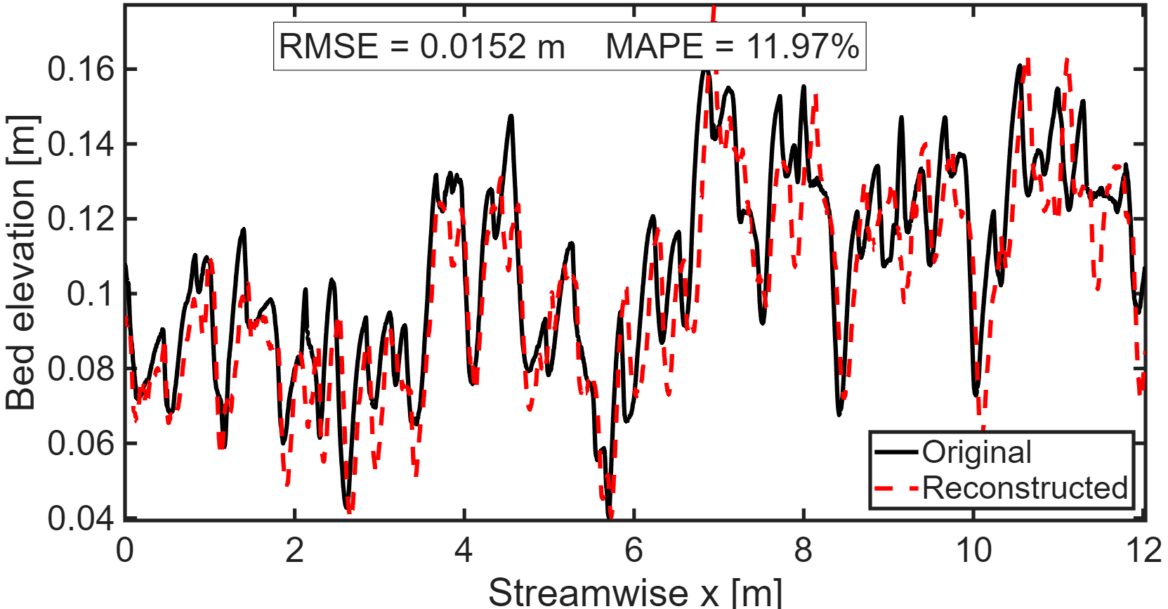
Figure 3 shows the DMD spectra. It also shows the periods associated with identified DMD eigenvalues. The periods were estimated using Equation 2. The size of the dots representing the eigenvalue is proportional to the DMD power associated with the mode. This helps identify the strength of the mode and its temporal period. In general, DMD eigenvalues are plotted on a unit circle. Since DMD eigenvalues exhibit symmetric behavior along x-axis, for brevity we plot only the upper half. We divide the semicircle into four regions based on periods. From left to right, along the semicircle, frequency decreases and time period increases. The divided regions are shown using separate envelopes. The figure illustrates the range of time periods in each envelope and the number of eigenvalues that fall inside the envelope. Here, if any eigenvalue ($\lambda$) varies by less than $1\%$, i.e., $0.99<|\lambda|<1.01$, we consider it to lie on the unit circle. Such an eigenvalue is associated with neither growth nor decay. In other words, it is considered persistent. On the other hand, eigenvalues that lie within the unit circle are shown with periods associated with them. These eigenvalues have relatively larger DMD power. Most of these eigenvalues are associated with modes shorter than $10$ minutes, indicating a fast-migrating and temporally decaying component of the bedform. In total, there are $12$ eigenvalues inside the unit circle, while $135$ eigenvalues lie on or outside the unit circle. The range $3.90-6\;\text{min}$ contains the majority of the periods ($N=47$), while only $9$ eigenvalues have periods longer than $1\;\text{hour}$. This indicates that bedform migration dynamics are primarily dominated by shorter periods or high-frequency components. To avoid clutter, we did not annotate individual periods on and outside the unit circle. Instead, the periods are represented using a color scale.

Figure 4 shows the reconstructed bed elevation at $y=63$ for the 150th time snapshot. The MAPE (mean absolute percentage error) estimated for that snapshot is $11.97\%$, showing the reconstruction accuracy of DMD. The figure shows that DMD is capable of visually reconstructing the bed elevation. The reconstruction was done using Equation 3. To examine the overall reconstruction performance, we estimated statistical measures of the reconstructed dynamics by computing the probability distribution function (PDF) and scatter plot. Figure 5(a) compares the original PDF and reconstructed PDF. It shows that the reconstructed PDF almost overlaps the original. Figure 5(b) shows the correlation between the original and the reconstructed elevation dynamics. Each point in the correlation signifies one point $\eta_{k}(x,t)$ of the bed elevation field at a particular instant. The correlation score is $0.9$, indicating the identified eigenvalues can accurately reconstruct the original dynamics. This is important in the sense that it ensures the system identification is justifiable.

Figure 6(a) shows the evolution of selected DMD modes at a particular point. The point is located at the center of the channel. The figure shows temporal evolution of elevation at that point. The black line represents the fluctuation of original elevation, while the colored lines show the temporal evolution of DMD modes associated with the point. Note that, in DMD, the mean is subtracted from the data. Therefore, DMD modes are computed from the fluctuations and compared with fluctuations rather than the raw elevation. Figure 6(b) characterizes the spatial behavior of the selected modes. Here we show the spatial component of the modes along one transect ($y=63$) at $150$th snapshot. The figure also illustrates the wavelengths associated with them. Note that the legend in Figure 6 (a) and Figure 6 (b) follows the same order.

IV Linking DMD and Sediment Flux via the Exner Equation

We begin with the two-dimensional Exner equation, which represents mass balance in sediment [13, 6, 10]:

$$(1-\lambda_{p})\,\frac{\partial\eta}{\partial t}\;+\;\nabla\!\cdot\vec{q}_{s}\;=\;0$$ (4)

where $\eta(x,y,t)$ is the bed elevation, $\lambda_{p}$ is the bed porosity, and $\vec{q}_{s}=(q_{s,x},q_{s,y})$ is the volumetric sediment flux vector. From DMD analysis in Section III, we obtain a linear, data-driven approximation of the temporal evolution of the topography. In continuous-time form we write

$$\frac{\partial\eta}{\partial t}\;\approx\;L\eta$$ (5)

where $L$ denotes the (linear) generator associated with the DMD model. In discrete time, DMD yields a matrix $A$ with eigenpairs $A\phi_{k}=\lambda_{k}\phi_{k}$; the corresponding continuous-time generator is related by $L=\tfrac{1}{\Delta t}\log(A)$, so that $L\phi_{k}=\omega_{k}\phi_{k}$ with $\omega_{k}=\log(\lambda_{k})/\Delta t$. Substituting (5) into (4) yields

$$(1-\lambda_{p})\,L\eta\;+\;\nabla\!\cdot\vec{q}_{s}\;=\;0\implies\nabla\!\cdot\vec{q}_{s}\;=\;-(1-\lambda_{p})\,L\eta.$$ (6)

To relate the DMD representation of $\eta$ to net streamwise flux through a cross-section at a fixed $y$, we integrate (6) in $x$ from $x_{\min}$ to $x_{\max}$:

$$\int_{x_{\min}}^{x_{\max}}\nabla\!\cdot\vec{q}_{s}(x,y,t)\,dx\;=\;-(1-\lambda_{p})\int_{x_{\min}}^{x_{\max}}(L\eta)(x,y,t)\,dx.$$ (7)

The left-hand side of the Exner equation can be written using the 2D divergence as:

$$\int_{x_{\min}}^{x_{\max}}\nabla\!\cdot\vec{q}_{s}(x,y,t)\,dx=\int_{x_{\min}}^{x_{\max}}\left(\frac{\partial q_{s,x}}{\partial x}+\frac{\partial q_{s,y}}{\partial y}\right)dx$$

$$=\frac{\partial}{\partial x}\left(\int_{x_{\min}}^{x_{\max}}q_{s,x}\,dx\right)+\frac{\partial}{\partial y}\left(\int_{x_{\min}}^{x_{\max}}q_{s,y}\,dx\right)$$

$$=q_{s,x}^{\mathrm{net}}(y,t)+\frac{\partial}{\partial y}\left(\int_{x_{\min}}^{x_{\max}}q_{s,y}\,dx\right).$$ (8)

We have defined the net streamwise flux through the transect as:

$$q_{s,x}^{\mathrm{net}}(y,t):=q_{s,x}(x_{\max},y,t)-q_{s,x}(x_{\min},y,t)$$

We obtain from Equation 8 and Equation 7

$$q_{s,x}^{\mathrm{net}}(y,t)+\frac{\partial}{\partial y}\!\left(\int_{x_{\min}}^{x_{\max}}q_{s,y}\,dx\right)=-(1-\lambda_{p})\int_{x_{\min}}^{x_{\max}}(L\eta)\,dx.$$ (9)

Since streamwise transport dominates and lateral flux variations are negligible, the $\partial_{y}$ term is commonly dropped. This yields the leading-order relation

$$q_{s,x}^{\mathrm{net}}(y,t)\;=\;-(1-\lambda_{p})\int_{x_{\min}}^{x_{\max}}(L\eta)\,dx.$$ (10)

We can express the reconstructed bed elevation as a superposition of DMD modes,

$$\eta(x,y,t)\approx\sum_{k}\alpha_{k}\phi_{k}(x,y)\,e^{\omega_{k}t}$$

where $\{\phi_{k}\}$ are (continuous-time) DMD modes, $\alpha_{k}$ are initial amplitudes, and $\omega_{k}$ are the associated continuous growth rates (units $[T]^{-1}$). Under the assumptions that (i) $L$ is linear and (ii) commuting $L$ and the $x$-integral is permissible, the right-hand side of (9) becomes

$$q_{s,x}^{\mathrm{net}}(y,t) \approx-(1-\lambda_{p})\!\int_{x_{\min}}^{x_{\max}}(L\eta)\,dx$$ (11)

$$\approx-(1-\lambda_{p})\!\sum_{k}\alpha_{k}e^{\omega_{k}t}\int_{x_{\min}}^{x_{\max}}L\phi_{k}(x,y)\,dx$$

$$\approx-(1-\lambda_{p})\!\sum_{k}\alpha_{k}e^{\omega_{k}t}\,\omega_{k}\int_{x_{\min}}^{x_{\max}}\phi_{k}(x,y)\,dx$$ (12)

Here, we used the eigenvalue relation $L\phi_{k}=\omega_{k}\phi_{k}$. Equation (12) shows that a weighted sum over DMD modes gives the net streamwise sediment flux through a transect. Each mode contributes in proportion to its integrated spatial mode shape over the transect, its modal amplitude, and its growth/decay rate $\omega_{k}$. We have assumed that cross-stream transport and its lateral gradient are negligible at the transect of interest.

Figure 7: Cumulative contribution of individual modes to total sediment transportation; the slowest 7 modes account for 50.9%, the fastest 120 modes contribute 25.7%, and all 147 modes explain 100% of transport.

V Discussion and Implications

In this section, we evaluate the implications of the mathematical derivation in Equation 12. The goal is to verify whether the surrogate measure of sediment flux estimated from DMD modes is consistent with the literature. By discarding the summation sign in Equation 12, we can write the contribution of each DMD mode $(\phi_{k})$ to the net sediment transport as $q_{s,x}^{k}(y,t,\phi_{k})=-(1-\lambda_{p})\alpha_{k}e^{\omega_{k}t}\,\omega_{k}\left(\int_{x_{\min}}^{x_{\max}}\phi_{k}(x,y)\,dx\right).$ Here, $q^{k}_{s,x}(y,t,\phi_{k})$ signifies the individual modal contribution to the net sediment flux, allowing the net flux to be decomposed into multiple spatial and temporal scales. The speed associated with each mode at a transect was estimated by computing its wavelength using spatial Fourier and Hilbert analysis, then multiplying it by the frequency obtained from the DMD eigenvalues.

The modes shown in Figure 6 were selected based on their contribution to sediment transport. The figure shows that slower modes contribute most individually, as $4$ of the $5$ modes depicted have a period longer than $1\;\text{hour}$. We sort the modes based on their speed and compute cumulative contributions by summing the sorted percentile contributions from the fastest to the slowest mode. This provides a clear visualization of how a small subset of modes dominates total sediment transport.

Figure 7 presents the cumulative contribution of individual modes to net sediment transport. The analysis shows that just the $7$ slowest modes account for $50.9\%$ of the total transport, while the remaining $140$ modes collectively contribute the other half. Moreover, the fastest $120$ modes, although numerous, contribute only $25.7\%$ in total. This indicates that sediment transport is dominated by a small number of slow, long-wavelength modes, whereas faster, short-wavelength modes provide a distributed but comparatively smaller contribution. Such behavior is consistent with recent studies showing that the spectral contribution of bedforms to sediment flux decreases with increasing frequency following a power-law scaling $q_{s}(f)\propto f^{-0.6}$ [9, 8]. Because low-frequency components correspond to large-scale, slowly migrating bedforms, this relationship implies that a small number of slow modes can carry a disproportionately large fraction of the sediment transport. In contrast, higher-frequency modes associated with smaller bedforms contribute more modestly despite their larger number. Unlike purely spectral approaches, the present DMD-based framework directly links sediment transport to dynamically evolving spatio-temporal modes of riverbed evolution, allowing the contribution of each mode to the net transport to be quantified explicitly.

VI Conclusion

In this paper, we present a novel data-driven framework for characterizing spatiotemporal mode-dependent sediment transport from riverbed topography. By substituting DMD modes of bed elevation into the Exner equation, we establish a physics-informed link between spatio-temporal modes and net sediment flux. Our analysis shows that the largest contributions to sediment transport come from slow, long-wavelength modes, while faster, small-wavelength modes, although individually smaller, are numerous and collectively influence transport dynamics. The analysis further reveals that persistent modes, characterized by DMD eigenvalues on the unit circle, act as the primary carriers of the bulk of the sediment flux. Thus, the proposed framework provides a non-intrusive surrogate for measuring sediment flux, offering new insights into the multiscale structure of bedform-driven transport. Future work will focus on extending the methodology to characterize sediment transport under different flow and channel conditions.

References

- [1] (2005) Effect of sampling time on measured gravel bed load transport rates in a coarse-bedded stream. Water Resources Research 41 (11). Cited by: §I.
- [2] (2020) A mixed length scale model for migrating fluvial bedforms. Geophysical Research Letters 47 (15), pp. e10–1029. Cited by: §I.
- [3] (2014) Spectral description of migrating bed forms and sediment transport. Journal of Geophysical Research: Earth Surface 119 (2), pp. 123–137. Cited by: §I.
- [4] (1971) Development and calibration of a pressure-difference bedload sampler. US Department of the Interior, Geological Survey, Water Resources Division. Cited by: §I.
- [5] (2018) Implications of the selection of a particular modal decomposition technique for the analysis of shallow flows. Journal of Hydraulic Research 56 (6), pp. 796–805. Cited by: §I.
- [6] (2005) A unified model for subaqueous bed form dynamics. Water Resources Research 41 (12). Cited by: §IV.
- [7] (2016) Dynamic mode decomposition: data-driven modeling of complex systems. SIAM. Cited by: §I, §III-A, §III-A.
- [8] (2022) Reconstructing sediment transport by migrating bedforms in the physical and spectral domains. Water Resources Research 58 (7), pp. e2022WR031934. Cited by: §I, §II, §V.
- [9] (2023) On the scaling and growth limit of fluvial dunes. Journal of Geophysical Research: Earth Surface 128 (6), pp. e2022JF006955. Cited by: §I, §I, §V.
- [10] (2009) Nature of deformation of sandy bed forms. Journal of Geophysical Research: Earth Surface 114 (F3). Cited by: §I, §IV.
- [11] (2022) A linear dynamical perspective on epidemiology: interplay between early covid-19 outbreak and human mobility. Nonlinear Dynamics 109 (2), pp. 1233–1252. Cited by: §III-A.
- [12] (2025) A koopman-theoretic approach to car-following and multi-lane interaction modeling. IEEE Open Journal of Intelligent Transportation Systems. Cited by: §III-A.
- [13] (2005) A generalized exner equation for sediment mass balance. Journal of Geophysical Research: Earth Surface 110 (F4). Cited by: §IV.
- [14] (2020) Entropy and intermittency of river bed elevation fluctuations. Journal of Geophysical Research: Earth Surface 125 (8), pp. e2019JF005499. Cited by: §I.
- [15] (2016) Correspondence between koopman mode decomposition, resolvent mode decomposition, and invariant solutions of the navier-stokes equations. Physical Review Fluids 1 (3), pp. 032402. Cited by: §I.
- [16] (1965) Bedload equation for ripples and dunes. US Government Printing Office. Cited by: §I.
- [17] (2009) Experimental evidence for statistical scaling and intermittency in sediment transport rates. Journal of Geophysical Research: Earth Surface 114 (F1). Cited by: §I.
- [18] (2012) Coupled dynamics of the co-evolution of gravel bed topography, flow turbulence and sediment transport in an experimental channel. Journal of Geophysical Research: Earth Surface 117 (F4). Cited by: §I.
- [19] (2011) Multiscale statistical characterization of migrating bed forms in gravel and sand bed rivers. Water Resources Research 47 (12). Cited by: §I.
- [20] (2006) Bed load bias: comparison of measurements obtained using two (76 and 152 mm) helley-smith samplers in a gravel bed river. Water Resources Research 42 (1). Cited by: §I.
- [21] (2016) Reduced sediment transport in the yellow river due to anthropogenic changes. Nature Geoscience 9 (1), pp. 38–41. Cited by: §I.