Movable-Antenna Index Modulation (MA-IM): System Framework and Performance Analysis

Abstract

This paper proposes a movable-antenna-based index modulation (MA-IM) framework that exploits the spatial mobility of a single reconfigurable antenna to create additional information-bearing dimensions for next-generation wireless systems. By discretizing the continuous movable region into a dense set of candidate sampling points and selecting representative anchors for indexing, the proposed framework converts spatial degrees of freedom into a practical modulation resource. Building on this framework, we develop a family of anchor-selection strategies with different levels of channel awareness, including geometry-based, SNR-based, max–min channel-domain, and joint constellation-aware designs. For the resulting MA-IM schemes, joint maximum-likelihood (ML) detectors are derived, along with a low-complexity two-stage detector, and unified analytical upper bounds on the average bit error probability (ABEP) are established based on the joint index–modulation constellation. The results reveal that directly indexing all sampling points is generally unreliable, highlighting the necessity of anchor optimization. The performance of MA-IM is shown to depend on key system parameters, including channel richness, spatial correlation, the number of index states, and the modulation order. In particular, increasing the number of index states and increasing the QAM order affect MA-IM in fundamentally different ways, even under the same transmission rate. Among the proposed schemes, the joint constellation-aware anchor design achieves the best error performance, demonstrating that optimizing channel-domain separation alone is insufficient and that effective MA-IM design must account for the geometry of the joint signal constellation. Simulation results further show that, with properly designed anchors, MA-IM can approach or even outperform same-spectral-efficiency QAM baselines.

I Introduction

In recent years, mobile communication systems have been rapidly evolving toward ultra-high capacity, ultra-low latency, and ultra-high energy efficiency [1]. However, traditional multi-antenna technologies such as multiple-input multiple-output (MIMO) and massive MIMO [2] are increasingly limited by hardware scalability, RF-chain cost, power consumption, and physical deployment constraints. Moreover, spectrum scarcity makes it difficult to meet future capacity demands merely by increasing modulation order or bandwidth. These trends call for new architectures that can enhance spectral and energy efficiency without additional hardware or power overhead [3, 4, 5].

To address the aforementioned challenges, a new class of reconfigurable antenna technologies has attracted significant interest. Reconfigurable intelligent surfaces (RIS) [6] enable programmable manipulation of the propagation environment through large arrays of nearly passive elements, whereas reconfigurable array antennas achieve flexible beamforming via switching networks or tunable components [7]. In parallel, fluid antennas (FA) [8, 9, 10] allow rapid relocation of the active port within a compact enclosure, effectively exploiting small-scale spatial channel fluctuations with extremely low hardware overhead. A more radical form of spatial reconfigurability is provided by movable antennas (MA) [11, 12, 13, 14], which physically reposition a single RF element within a bounded 2D/3D/6D region. Unlike conventional fixed-geometry antennas (FGA), both FA and MA convert the spatial position itself into a controllable communication resource, enabling the system to probe or select favorable channel realizations without increasing the number of RF chains, transmit power, or antenna aperture. This spatial mobility provides several notable advantages: (i) access to rich channel diversity at minimal hardware cost; (ii) position-domain scheduling for improved signal-to-noise ratio (SNR) or lower correlation; and (iii) channel-shaping capabilities comparable to MIMO or RIS but with substantially lower energy consumption. Consequently, FA and MA, alongside RIS and MIMO, are emerging as key enablers of 6G reconfigurable spatial communications, with promising applications in integrated sensing and communication (ISAC), cooperative networks, and green wireless systems [15, 16, 17, 18].

Meanwhile, index modulation (IM) [19] has emerged as an effective technique for improving spectral efficiency (SE) and reducing hardware cost by conveying information through an additional index dimension. The key idea of IM is to activate or select certain entities, such as antennas, subcarriers, time slots, carrier frequencies, or channel states [20, 21, 22], thereby enabling the transmission of extra bits beyond conventional signal constellations. As a result, IM can enhance SE without increasing the modulation order, making it attractive for green communication systems with strict hardware and energy constraints.

IM has been widely integrated into fixed-antenna architectures. A representative example is spatial modulation (SM) [23], which conveys index bits via antenna activation. Numerous extensions, including generalized SM (GSM) [24], quadrature SM (QSM) [25], enhanced SM (ESM) [26], and precoding SM (PSM) [27], further improve SE and reliability through richer activation patterns and advanced processing techniques. Beyond conventional MIMO systems, IM has also been combined with emerging architectures. For instance, frequency diverse arrays (FDA) [28] introduce additional index dimensions across frequency and spatial domains [29, 30, 31, 32]. In mmWave systems, spatial scattering modulation (SSM) [33] exploits sparse propagation paths for index transmission, while its extension, polarized SSM (PSSM) [34], further leverages polarization diversity.

Despite these advances, most existing IM schemes rely on fixed-position antenna architectures (FPA-IM), whose index space is fundamentally constrained by the physical antenna layout, limiting scalability in the spatial domain. To overcome this limitation, recent works have explored IM with reconfigurable antenna structures such as RIS and FA [35]. In particular, FA-enabled IM schemes have been proposed for MIMO systems [36], grouping-based designs [37], and position-domain index modulation [38], demonstrating improved SE and robustness. Furthermore, continuous-trajectory FA (CT-FA) based IM [39] exploits channel variations induced by antenna motion to enable covert communication.

Despite the demonstrated potential of MA in enhancing spatial degrees of freedom and improving channel reconfigurability, to the best of the authors’ knowledge, no existing work has systematically integrated the spatial mobility of MA with the IM framework. In particular, the literature lacks a unified study on how to construct index states from the continuous two-dimensional movable region of an MA, nor does it provide corresponding modulation schemes, detection algorithms, or performance analyses tailored for such systems. This clear research gap presents a timely opportunity to explore the synergy between MA and IM.

Motivated by this observation, combining the spatial mobility of MA with the indexing principle of IM opens up an entirely new modulation dimension, where the physical position of the antenna itself serves as a controllable information-bearing resource. Such a hybrid architecture can enhance SE without requiring additional RF chains or expanded bandwidth, while exploiting the rich channel diversity induced by MA movement. To fully leverage this new modulation dimension, it is essential to carefully reconcile the discrete nature of IM with the intrinsically continuous spatial mobility of MA. In this regard, although IM introduces discrete index states, the proposed MA-IM framework does not quantize the antenna motion itself at a conceptual level. Instead, the intrinsic continuous spatial degrees of freedom of MA are preserved through dense spatial sampling and channel-domain design, which enables MA-IM to retain the fundamental characteristics of MA systems. However, the integration of continuous spatial mobility with discrete index modulation gives rise to two fundamental challenges.

• How to discretize the continuous movable region into a finite set of sampling points? The MA operates over a continuous spatial region, whereas IM inherently relies on discrete states. Therefore, it is necessary to construct a sufficiently dense set of sampling points to approximate the continuous spatial domain, while preserving the underlying channel variations induced by antenna movement.

• How to select representative sampling points for reliable index modulation? Although dense spatial sampling captures the continuous nature of MA, directly indexing all sampling points is generally unreliable due to strong spatial correlation, which leads to poor distinguishability among index states. Therefore, it is essential to select a subset of representative sampling points that maximizes channel separability and enables reliable index detection.

To overcome these challenges, this paper presents a novel MA-based index modulation framework and makes the following key contributions:

• We develop a practical MA-IM system model that converts the continuous movable region of the antenna into a discrete set of candidate transmission positions through dense spatial sampling. This discretization reveals a large pool of channel realizations induced by the MA mobility and provides a foundation for constructing index-modulated transmission states.

• We introduce the concept of anchor selection for MA systems. Unlike conventional FA-IM schemes that assume a predefined set of antenna ports and only perform indexing among them, the proposed framework first selects a subset of representative ports (anchors) from a dense set of candidate MA sampling locations. This additional design freedom allows the system to exploit the underlying channel geometry and significantly improve the separability among index states.

• Based on the proposed anchor-selection framework, we develop a family of MA-IM schemes with progressively increasing levels of channel awareness, including random activation, geometry-based selection, SNR-based representative selection, cell-constrained max–min design, global max–min optimization, and joint constellation-distance-aware anchor selection. These schemes form a unified design hierarchy that systematically enhances the separability of index states in the channel domain and, ultimately, in the joint index–modulation constellation. This framework enables a comprehensive performance comparison across geometry-driven, channel-aware, and constellation-aware port selection strategies.

• For the resulting MA-IM transmission schemes, we derive joint maximum-likelihood (ML) detectors that simultaneously estimate the active index state and the transmitted QAM symbol. In addition, tight union-bound expressions of the average bit error probability (ABEP) are obtained for representative schemes, enabling analytical performance characterization under various system parameters.

• To reduce the computational burden of exhaustive ML detection, we further design a low-complexity two-stage detector that achieves a favorable performance–complexity tradeoff and makes MA-IM suitable for practical implementation.

• Extensive Monte Carlo simulations validate the accuracy of the derived ABEP expressions and demonstrate that the proposed channel-aware anchor selection strategies significantly improve the reliability of MA-IM systems. The results also provide useful design guidelines on sampling density, index alphabet size, and modulation order for MA-enabled communication systems.

Overall, the results demonstrate that MA-IM can effectively exploit spatial reconfigurability to enhance modulation dimensionality and system performance without increasing hardware complexity. The proposed framework offers new insights and practical methodologies for the design of next-generation green, SE, and reconfigurable wireless communication systems.

The remainder of this paper is organized as follows. Section II establishes the overall MA-based transmission framework. Besides, a family of anchor-selection strategies for constructing index-modulated transmission states are given in Section III. Section IV presents the corresponding joint ML detectors for all schemes and develops a low-complexity two-stage detection algorithm. Section V provides a comprehensive performance analysis, including the achievable throughput and the derived ABEP upper bounds. Section VI reports extensive simulation results that validate the theoretical findings. Finally, Section VII concludes the paper and outlines several promising future research directions.

II System Model and Movable Antenna Discretization

The MA-IM system investigated in this paper is depicted in Fig. 1. At the transmitter, a MA is employed, whereas the user adopts conventional FPA such as phase array (PA). The MA module is connected to the RF chain through flexible coaxial cables, thereby enabling real-time and continuous adjustment of its spatial position. Let the position of an MA be represented by the Cartesian coordinate vector $\boldsymbol{t}=[x,y]^{T}\in\mathcal{C},$ where $\mathcal{C}$ denotes the designated two-dimensional (2D) region within which the transmit MA is allowed to move freely without mechanical constraints. Throughout this work, we focus on narrowband and quasi-static channel conditions. We further assume that the MA can relocate with sufficiently high agility such that the positioning overhead is negligible relative to the extended channel coherence time, thus ensuring that MA reconfiguration does not disrupt communication [40].

Figure 1: System model of the proposed MA-IM framework.

II-A Channel model

The channel vector between the MA-IM transmitter and the user is determined by both the propagation environment and the positions of the MA. Since the movement range of the antennas is negligible compared with the signal propagation distance, the far-field assumption is adopted. Based on this assumption, the MA–PA channels can be modeled using the plane-wave approximation [41]. Consequently, for each propagation path, the complex path coefficients at different MA locations exhibit different phases. This property allows the spatial variation of the channel to be fully characterized by the phase term induced by the propagation distance difference.

Figure 2: Illustration of the spatial angle domain corresponding to the transmit region

Assume that the number of propagation paths is $L$. As illustrated in Fig. 2, the $l$-th path is characterized by its elevation and azimuth angles of departure (AoD), denoted by $\theta^{l}$ and $\phi^{l}$, respectively. The corresponding 3D unit propagation direction can be defined according to the geometric coordinate system in Fig. 2. Since MA is restricted to a 2D transmit region, only the projection of the propagation direction onto this region is relevant for characterizing the phase variation across different MA positions.

Accordingly, the effective 2D wavefront vector of the $l$-th path on the transmit region is written as $\boldsymbol{n}^{l}=\left[\sin\theta^{l}\cos\phi^{l},\cos\theta^{l}\right]^{T}$.

Let the origin of the MA region be $\boldsymbol{o}=[0,0]^{T}$, and let $\boldsymbol{t}=[x,y]^{T}$ denote an arbitrary transmit position on the 2D region. Under the plane-wave assumption, the path-length difference of the $l$-th propagation path between $\boldsymbol{t}$ and $\boldsymbol{o}$ is given by the projection of the displacement $\boldsymbol{t}-\boldsymbol{o}$ onto the effective wavefront vector, i.e.,

$$\rho^{l}(\boldsymbol{t})=(\boldsymbol{n}^{l})^{T}(\boldsymbol{t}-\boldsymbol{o})=x\sin\theta^{l}\cos\phi^{l}+y\cos\theta^{l}.$$ (1)

Thus, the field-response vector characterizing the transmit MA is defined as [42]

$$\boldsymbol{f}\left(\boldsymbol{t}\right)=\left[e^{j\frac{2\pi}{\lambda}\rho^{1}\left(\boldsymbol{t}\right)},e^{j\frac{2\pi}{\lambda}\rho^{2}\left(\boldsymbol{t}\right)},\cdots,e^{j\frac{2\pi}{\lambda}\rho^{L}\left(\boldsymbol{t}\right)}\right]^{T}\in\mathbb{C}^{L},$$ (2)

with the symbol $\lambda$ denoting the wavelength.

II-B Port discretization

To facilitate theoretical analysis and performance evaluation, this paper introduces a sampled MA model. Instead of allowing the MA to move continuously over the region $\mathcal{C}$, we approximate this continuous area using a sufficiently dense set of discrete sampling points. Formally, the continuous movement space is discretized into a finite set $\mathcal{C}_{d}=\left\{\mathbf{t}_{1},\mathbf{t}_{2},\dots,\mathbf{t}_{Q}\right\}$ with $Q$ being the total sampling number, and the MA is assumed to move among these discrete points. This discretization converts the original continuous-position selection problem into a finite-state switching problem, significantly simplifying the modeling and analysis.

As long as the sampling points are dense enough, the discrete points can accurately capture the spatial phase variations and channel fluctuations over the continuous region. Therefore, the sampled points serve as a high-fidelity approximation of the continuous MA movement space, without sacrificing the spatial degrees of freedom or channel diversity gains inherent to MA.

Moreover, this sampled MA abstraction is also aligned with practical hardware implementations. Whether the MA is driven by mechanical actuators (e.g., linear rails or stepper motors) or realized through micro-electro-mechanical systems (MEMS)/liquid-metal mechanisms as in FA, the physically reachable antenna positions are inherently discrete with finite spatial resolution. Furthermore, under the sampling-theoretic constraints, Lemma 1 provides the maximum allowable sampling interval for discretizing the movable-antenna region, thereby offering a theoretical guideline for constructing a finite set of sampling points from the original continuous movement space.

Lemma 1.

Consider a rich-scattering environment where the spatial correlation between two antenna positions separated by distance $\Delta r$ is approximated by [43, 44]

$$\rho(\Delta r)=J_{0}\!\left(\frac{2\pi\Delta r}{\lambda}\right),$$ (3)

where $J_{0}(\cdot)$ denotes the zeroth-order Bessel function. Given a target correlation level $\rho_{\mathrm{tar}}\in[0,1)$, the maximum spacing $\Delta r_{\max}$ that guarantees $\rho(\Delta r)\geq\rho_{\mathrm{tar}}$ is

$$\Delta r_{\max}\approx\frac{\lambda}{\pi}\sqrt{1-\rho_{\mathrm{tar}}}.$$ (4)

Proof.

Using the approximation $J_{0}(x)\approx 1-x^{2}/4$ for small $x$, we obtain

$$\rho(\Delta r)\approx 1-\frac{1}{4}\!\left(\frac{2\pi\Delta r}{\lambda}\right)^{2}.$$ (5)

Imposing $\rho(\Delta r)\geq\rho_{\mathrm{tar}}$ leads to

$$1-\frac{1}{4}\!\left(\frac{2\pi\Delta r}{\lambda}\right)^{2}\geq\rho_{\mathrm{tar}},$$ (6)

which gives

$$\Delta r_{\max}\approx\frac{\lambda}{\pi}\sqrt{\,1-\rho_{\mathrm{tar}}\,}.$$ (7)

This completes the proof. ∎

Compared with the Nyquist sampling limit $\lambda/2$, the spacing $\Delta r_{\max}$ derived in Lemma 1 based on channel-similarity constraints is strictly smaller. Consequently, the admissible sampling intervals for discretizing the movable-antenna region along the $x$– and $y$–directions can be written as:

$$dx\in\left[0,\Delta r_{\max}\right],\quad dy\in\left[0,\Delta r_{\max}\right].$$ (8)

(8) indicates that as the sampling interval approaches zero, the movable-antenna region effectively behaves as a continuous domain. However, to ensure the target channel similarity $\rho_{\mathrm{tar}}$, the sampling interval must be bounded above by $\Delta r_{\max}$. In the subsequent section, to simplify the analysis and highlight the key performance trends, we set $d_{x}$ and $d_{y}$ to their maximum allowable values.

Figure 3: Illustration of the sampling layout in the MA region under the target channel similarity constraint $\rho_{\mathrm{tar}}=0.9$.

Fig. 3 shows all sampling points within the MA’s movable region under the design target $\rho_{\mathrm{tar}}=0.9$. The channel similarity between any two positions $\boldsymbol{t}_{m}$ and $\boldsymbol{t}_{n}$ is defined as

$$\rho_{h}=\boldsymbol{f}(\boldsymbol{t}_{m})^{\dagger}\boldsymbol{f}(\boldsymbol{t}_{n})/L.$$ (9)

By computing the similarity for all adjacent sampling-point pairs in Fig. 3 and taking the average, an averaged similarity of $\rho_{h}=0.8945$ is obtained, indicating that the corresponding channels are highly correlated. This observation further confirms the validity of the proposed lemma.

III Index modulation scheme

Building upon the above discretization and partitioning framework, a straightforward approach is to directly treat all sampled MA positions as candidates for index modulation. From an information-theoretic perspective, such a design maximizes the number of index states and thus increases the achievable index modulation rate. However, directly indexing all sampled positions is generally undesirable in practice. As the indexed positions become denser, the spatial separation between adjacent positions decreases, and the resulting channel responses become increasingly similar. This reduces the distinguishability among index states in the channel domain and makes reliable detection at the receiver more challenging, thereby leading to a higher bit error rate (BER).

Therefore, it is essential to select a subset of representative sampling points for IM. The objective is to enhance the distinguishability among index states and improve the reliability of ML detection. The primary focus of this work is on how to design such representative anchor selection strategies. Hence, we develop a family of MA-IM schemes that differ in their representative port selection strategies.

As a baseline, a random activation scheme is considered, where the MA can move freely within the selected mobility block. A geometry-based scheme then fixes the MA at the geometric center of each block, providing a deterministic representative position. To further exploit channel variations, an SNR-based scheme selects the port with the largest channel gain within each block. In addition, a distance-based scheme employs a max–min (i.e., maximizing the minimum pairwise channel distance, which is sometimes referred to as a min–max formulation in related literature [45]) criterion to select the representative port that maximizes the minimum channel distance among different index states within each block. Next, we consider a channel-domain anchor design that removes the geometric partition constraint and directly selects representative ports according to a global max–min channel-distance criterion. Furthermore, to fully capture the joint effect of index selection and signal modulation, we propose a constellation-aware anchor design, which directly optimizes the minimum Euclidean distance of the resulting joint index–modulation constellation, thereby achieving significantly improved detection performance.

III-A Random activation (Scheme 1)

In this scheme, we first divide the 2D movable region of the MA into $N=N_{1}\times N_{2},$ where $N_{1}$ and $N_{2}$ denote the numbers of grids along the horizontal and vertical directions, respectively. To ensure distinct MA-IM states, the condition $N<Q$ must be satisfied. This raises a practical question: when a grid index is selected for transmission, which sampling point within that grid should be used as the actual MA position?

The movable region is partitioned into $N$ geometric cells, and the $c$-th cell contains a set of candidate sampling points denoted by $\mathcal{S}_{c}$. In this scheme, the transmit position is randomly selected from the candidate points inside the activated cell, i.e.,

$$q_{\mathrm{tx}}\sim\mathrm{Unif}\big(\mathcal{S}_{c}\big),$$ (10)

and the MA transmits from the corresponding physical coordinate $\boldsymbol{t}_{q_{\mathrm{tx}}}$ with $\mathrm{Unif}(\cdot)$ denoting a uniform random selection from the specified set .

Let $\boldsymbol{h}_{q}\triangleq\boldsymbol{f}(\boldsymbol{t}_{q})\in\mathbb{C}^{N_{r}}$ be the corresponding channel vectors. Consequently, the received signal $\boldsymbol{y}\in\mathbb{C}^{N_{r}\times 1}$ can be written as

$$\boldsymbol{y}=E_{s}s\,\boldsymbol{h}_{q_{\mathrm{tx}}}+\boldsymbol{n}.$$ (11)

Here, $E_{s}$ denotes the transmit energy per symbol and $\boldsymbol{n}\in\mathbb{C}^{N_{r}\times 1}$ is the complex additive white Gaussian noise (AWGN), satisfying $\boldsymbol{n}\sim\mathcal{CN}(0,N_{0}\boldsymbol{I})$. Moreover, $s\in\mathcal{S}_{M}$ denotes the transmitted modulation symbol drawn from an $M$-QAM constellation, where $|\mathcal{S}_{M}|=M$ and $\mathbb{E}[|s|^{2}]=1$.

Although Scheme 1 reflects the random mobility of the movable antenna, the unknown transmit position within each cell leads to unreliable demodulation and degraded BER performance. Therefore, it mainly serves as a baseline to motivate anchor-based designs, which aim to improve the reliability of index transmission.

III-B Geometry-based anchoring (Scheme 2)

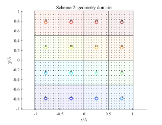
To address the randomness and unreliability of Scheme 1, a natural idea is to assign a deterministic representative transmit position to each cell. A simple yet intuitive choice is to exploit the geometric structure of the partition. In Scheme 2, each cell is represented by a fixed anchor point determined based on the geometric structure of the partition.

Let $\mathbf{c}_{c}$ denote the geometric center of the $c$-th cell and let $\mathbf{t}_{q}$ denote the coordinate of the $q$-th sampling point. The representative port of cell $c$ is selected as the sampling point closest to the cell center. Hence, the representative anchor point $a_{c}$ is chosen as

$$a_{c}=\arg\min_{q\in\mathcal{S}_{c}}\bigl\|\boldsymbol{t}_{q}-\boldsymbol{c}_{c}\bigr\|^{2}$$ (12)

Thus, each grid is represented by a unique anchor point, which serves as the actual MA transmit location for that grid, as shown in Fig. 4.

Figure 4: Example of MA indexing: each block corresponds to one index value, and the colored point denotes the selected physical transmit coordinate for that index.

Consequently, IM operates directly on this set of anchors. Based on Fig. 1, the incoming bitstream can therefore be partitioned into two sub-vectors of lengths $\log_{2}M\quad$ and $\left\lfloor\log_{2}N\right\rfloor$ denoted as $\boldsymbol{p}_{1}$ and $\boldsymbol{p}_{2}$. The bits in $\boldsymbol{p}_{1}$ are mapped to an $M$-QAM symbol $s$, whereas the IM bits in $\boldsymbol{p}_{2}$ are used to select a unique MA position pattern $I=\{1,2,\ldots,N\}.$

Let $\mathcal{A}=\{a_{1},a_{2},\ldots,a_{C}\}$ denote the set of anchor indices, where $a_{c}$ corresponds to the representative sampling point selected in the $c$-th cell. When the index state $c$ is activated, the MA directly transmits from the anchor position $\boldsymbol{t}_{a_{c}}$.

The received signal $\boldsymbol{y}\in\mathbb{C}^{N_{r}}$ can therefore be written as

$$\boldsymbol{y}=E_{s}s\,\boldsymbol{h}_{a_{c}}+\boldsymbol{n}.$$ (13)

While Scheme 2 assigns a deterministic anchor to each cell based purely on geometric proximity, the resulting anchor positions do not necessarily correspond to favorable channel conditions. In practical wireless environments, the channel strength may vary significantly across different sampling points within the same cell due to multipath propagation and small-scale fading. As a result, selecting the geometric center as the representative position may lead to suboptimal transmission reliability.

To address this limitation, we next consider a channel-aware representative selection strategy that exploits the instantaneous channel strength within each cell.

III-C SNR-based selection (Scheme 3)

To improve the reliability of index transmission while preserving the geometric partition structure, we consider a representative port selection strategy based on the instantaneous channel strength within each cell. This scheme is referred to as Scheme 3.

Hence, the representative port for the $c$-th cell is selected as the port with the largest channel gain within that cell, i.e.,

$$q_{c}^{\star}=\mathrm{arg}\max_{q\in\mathcal{S}_{c}}|\boldsymbol{h}_{q}|^{2}.$$ (14)

To facilitate practical implementation, the SNR-based representative selection procedure is summarized in Algorithm 1. The algorithm simply scans all candidate ports within each cell and selects the port with the maximum channel gain as the representative position.

The selected representative ports form the set

$$\mathcal{B}=\{q_{1}^{\star},q_{2}^{\star},\dots,q_{C}^{\star}\}.$$

The effective channel corresponding to the $c$-th index state is therefore $\tilde{\boldsymbol{h}}_{c}=\boldsymbol{h}_{q_{c}^{\star}}.$

Compared with the geometry-based scheme (Scheme 2), Scheme 3 improves the received signal quality by selecting the strongest port in each cell, thereby increasing the effective SNR for each index state.

When the $c$-th index state is activated, the transmitted signal experiences the effective channel $\tilde{\boldsymbol{h}}_{c}$. The received signal can be expressed as

$$\boldsymbol{y}=E_{s}s\tilde{\boldsymbol{h}}_{c}+\boldsymbol{n}.$$ (15)

Algorithm 1 Cell-wise SNR-Based Representative Selection (Scheme 3)

0: Candidate port sets $\{\mathcal{S}_{c}\}_{c=1}^{C}$, channel coefficients $\{h_{q}\}$

0: Representative ports $\{q_{c}^{\star}\}_{c=1}^{C}$

1: for $c=1$ to $C$ do

2:  $q_{c}^{\star}=\arg\max_{q\in\mathcal{A}_{c}}|h_{q}|^{2}$

3: end for

4: return $\{q_{c}^{\star}\}$

Figure 5: Example of MA indexing under Scheme 3. Black dots denote candidate sampling positions, while colored circles indicate the selected representative ports in each cell.

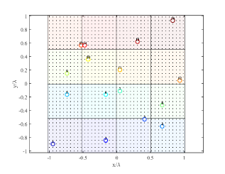
Fig. 10 illustrates the representative ports selected under Scheme 3. The MA region is first partitioned into multiple geometric cells, where each cell corresponds to one index state. Within each cell, the sampling point with the strongest channel gain is chosen as the representative transmit position according to (14). The black dots denote all candidate sampling positions, while the colored circles indicate the selected representative ports. Compared with geometry-based anchoring, this channel-aware selection strategy improves the effective SNR associated with each index state and therefore enhances the reliability of index detection.

While Scheme 3 selects the representative port in each cell based on the strongest channel gain, this criterion focuses on improving the signal strength of individual index states rather than their mutual distinguishability. As a result, the selected ports from different cells may still produce highly correlated channel responses, which limits the separability of the resulting index states.

To address this limitation, we next consider a representative selection strategy that explicitly maximizes the minimum pairwise channel distance among the selected ports.

III-D Distance-based selection (Scheme 4)

To further improve the distinguishability among different index states while preserving the geometric partition structure, we consider a cell-constrained max–min representative selection strategy, referred to as Scheme 4.

Unlike Scheme 3, which selects the representative port in each cell based on the strongest channel gain, the proposed Scheme 4 explicitly considers the separability among different index states. Specifically, one representative port is deterministically selected from each cell such that the minimum pairwise channel distance among all selected ports is maximized. In this respect, the representative ports are obtained by solving

$$\{q_{1}^{\star},\dots,q_{C}^{\star}\}=\arg\max_{q_{1}\in\mathcal{S}_{1},\dots,q_{C}\in\mathcal{S}_{C}}\min_{i\neq j}|\boldsymbol{h}_{q_{i}}-\boldsymbol{h}_{q_{j}}|.$$ (16)

The optimization in (16) ensures that the channel states associated with different index positions are well separated in the complex channel space, thereby improving the distinguishability of different index states.

However, directly solving the combinatorial optimization in (16) is computationally prohibitive when the number of candidate ports is large. To address this issue, we propose a greedy cell-constrained search algorithm to compute the representative ports $\{q_{1}^{\star},\dots,q_{C}^{\star}\}$. The procedure is summarized in Algorithm 2.

Algorithm 2 Greedy Cell-Constrained Max–Min Representative Selection (Scheme 4)

0: Candidate port sets $\{\mathcal{S}_{c}\}_{c=1}^{C}$, channel coefficients $\{\boldsymbol{h}_{q}\}_{q=1}^{Q}$, maximum iteration number $I_{\max}$

0: Representative ports $\{q_{c}^{\star}\}_{c=1}^{C}$

1: Initialize representative ports $q_{c}^{(0)}\in\mathcal{S}_{c}$ using geometric anchors

2: Set iteration index $i=0$

3: repeat

4:  for $c=1$ to $C$ do

5:   Fix representatives of other cells $\{q_{j}\}_{j\neq c}$

6:   for each candidate $q\in\mathcal{S}_{c}$ do

7:    Compute distance metric

$$\eta_{c}(q)=\min_{j\neq c}|\boldsymbol{h}_{q}-\boldsymbol{h}_{q_{j}}|$$

8:   end for

9:   Update representative

$$q_{c}^{(i+1)}=\arg\max_{q\in\mathcal{S}_{c}}\eta_{c}(q)$$

10:  end for

11:  $i\leftarrow i+1$

12: until convergence or $i=I_{\max}$

13: $q_{c}^{\star}=q_{c}^{(i)}$

Once the representative ports set $\mathcal{C}=\{q_{c}^{\star}\}_{c=1}^{C}$ are determined, the effective channel corresponding to the $c$-th index state is given by $\bar{\boldsymbol{h}}_{c}=\boldsymbol{h}_{q_{c}^{\star}}.$

The received signal can be written as

$$\boldsymbol{y}=E_{s}s\bar{\boldsymbol{h}}_{c}+\boldsymbol{n}.$$ (17)

Figure 6: Example of MA indexing under Scheme 4. Black dots denote candidate sampling positions, while colored circles indicate the selected representative ports in each cell.

Fig. 6 shows the representative ports obtained by Scheme 4. Compared with Fig. 5, most representative ports are different because Scheme 4 optimizes the minimum channel distance among index states rather than the individual channel strength. Nevertheless, a few representative ports coincide with those in Scheme 3, indicating that the strongest channel position may also yield good channel separability in certain cells.

The previous schemes (Schemes 1–4) share a common design principle in that the movable region is first partitioned into geometric cells and one representative port is selected from each cell. Although different criteria are used for representative selection (random sampling, geometric anchoring, SNR maximization, and max–min channel separation), the underlying geometric partition constraint remains unchanged.

However, the wireless channel induced by MA may vary highly non-uniformly across space, and spatial proximity does not necessarily imply channel similarity. Consequently, restricting the anchor positions to predefined geometric cells may limit the achievable channel separability among index states.

Motivated by this observation, we next consider a channel-domain anchor design strategy that removes the geometric partition constraint and directly optimizes the anchor positions according to channel dissimilarity.

III-E Channel-domain max–min anchor design (Scheme 5)

Unlike Schemes 1–4, which follow a cell-constrained design based on geometric partitioning of the movable region, Scheme 5 constructs the index states directly in the channel domain. The key motivation is that MA-induced channels may vary highly non-uniformly across space, whereas geometric partitioning imposes a uniform spatial grid that does not necessarily reflect the underlying channel structure.

Consequently, spatially adjacent cells in Schemes 1–4 may still correspond to highly similar channel responses. In such cases, the minimum separation between anchor channels is essentially limited by the grid resolution. When the number of index states $N$ increases, the geometric cells must shrink accordingly, which inevitably reduces the minimum channel distance between neighboring anchors and leads to a denser joint constellation, thereby degrading the reliability of index detection.

In contrast, Scheme 5 does not rely on geometric proximity. Instead, it explicitly selects anchor positions based on channel dissimilarity and aims to maximize the minimum pairwise channel distance among the chosen anchors. This max–min criterion ensures that the resulting anchor channels are as mutually distinguishable as possible, yielding a joint constellation with significantly larger minimum Euclidean distance and thereby substantially more robust ML demodulation.

We seek an anchor set

$$\mathcal{D}=\{a_{1},a_{2},\ldots,a_{N}\}\subseteq\{1,2,\ldots,Q\},$$ (18)

that maximizes the minimum channel separation, namely

$$\max_{\mathcal{D}:\,|\mathcal{D}|=N}\;\min_{i\neq j}\big\|\boldsymbol{h}_{a_{i}}-\boldsymbol{h}_{a_{j}}\big\|.$$ (19)

This max–min criterion is aligned with classical codebook optimization and directly improves the minimum distance of the joint constellation, which in turn lowers the ABEP union bound and the BER.

Since the combinatorial problem (19) is NP-hard [46], we employ the farthest-point sampling (FPS) strategy, which provides an effective greedy approximation [47]. The procedure is summarized in Algorithm 3.

Algorithm 3 Max–min channel-domain anchor selection via farthest-point sampling

0: Complex channel samples $\{\boldsymbol{h}_{q}\}_{q=1}^{Q}$, target number of anchors $N$

0: Anchor index set $\mathcal{D}=\{a_{1},\ldots,a_{N}\}$

1:  Step 1: Pre-compute pairwise channel distances

2: for $q_{1}=1$ to $Q$ do

3:  for $q_{2}=1$ to $Q$ do

4:   $D(q_{1},q_{2})=|\boldsymbol{h}_{q_{1}}-\boldsymbol{h}_{q_{2}}|$

5:  end for

6: end for

7:  Step 2: Initialize the first anchor

8: Compute the average distance of each point: $\bar{d}(q)=\frac{1}{Q-1}\sum_{q^{\prime}\neq q}D(q,q^{\prime})$

9: Select the point with the largest average distance: $a_{1}=\arg\max_{q}\bar{d}(q)$

10: $\mathcal{D}\leftarrow\{a_{1}\}$

11:  Step 3: Iteratively select the remaining $C-1$ anchors

12: for $c=2$ to $N$ do

13:  for each $q\in\{1,\ldots,Q\}$ do

14:   Compute the distance to current anchor set:

$$d_{\min}(q)=\min_{a\in\mathcal{D}}D(q,a)$$

15:  end for

16:  Exclude already selected anchors by setting $d_{\min}(a)=0$ for all $a\in\mathcal{D}$

17:  Select the farthest point:

$$a_{c}=\arg\max_{q}d_{\min}(q)$$

18:  Update: $\mathcal{D}\leftarrow\mathcal{D}\cup\{a_{c}\}$

19: end for

20: return $\mathcal{D}$

Furthermore, Fig. 7 shows the anchors obtained by Algorithm 3. Compared with the geometry-driven distribution in Fig. 4, the anchors selected by Scheme 5 are determined entirely in the channel domain and are therefore not constrained by the geometric grid. As a result, the spatial spacing among anchors is adaptively adjusted according to channel dissimilarity. This can be clearly observed in Fig. 7, where geometrically close positions may correspond to highly distinct channel realizations, while the smallest channel distance may occur between positions that are not spatially adjacent. Such behavior highlights the benefit of channel- domain anchor design in enlarging the minimum channel separation among index states.

Figure 7: Geometry-domain visualization of the max–min anchor selection. Black dots represent all sampled MA positions, while colored circles indicate the selected $N$ anchors.

Once the anchor set $\mathcal{D}$ is obtained, the MA activates the position $\boldsymbol{t}_{a_{I}}$ corresponding to the selected index $I$ and transmits symbol $s$. The received signal is then

$$\boldsymbol{y}=E_{s}s\,\boldsymbol{h}_{a_{I}}+\boldsymbol{n}.$$ (20)

For the anchor set $\mathcal{D}$, we define the minimum channel separation as

$$d_{\min}^{h}=\min_{i\neq j}\big\|\boldsymbol{h}_{a_{i}}-\boldsymbol{h}_{a_{j}}\big\|.$$ (21)

Although the overall ABEP of MA-IM with QAM is determined by the Euclidean distances of the joint constellation points $\{\boldsymbol{h}_{a_{i}}s_{m}\}$, the channel-side metric $d_{\min}^{h}$ provides a useful measure of the distinguishability between index states.

In particular, when the same QAM symbol is transmitted from two different anchors, the corresponding pairwise distance becomes $|s_{m}|\,\|\boldsymbol{h}_{a_{i}}-\boldsymbol{h}_{a_{j}}\|$. Therefore, increasing $d_{\min}^{h}$ generally improves the separability of index states and reduces the probability of index-detection errors. However, the overall BER performance ultimately depends on the geometry of the joint constellation $\{\boldsymbol{h}_{a_{i}}s_{m}\}$, which motivates the constellation-aware anchor optimization introduced in Scheme 6.

III-F Joint constellation–distance anchoring (Scheme 6)

Scheme 5 selects anchor ports by maximizing the minimum separation between channel vectors, i.e., $\min_{i\neq j}\|\boldsymbol{h}_{i}-\boldsymbol{h}_{j}\|$. However, the detection performance of IM is ultimately determined by the Euclidean distance between the received signal constellation points.

To better align the anchor design with the BER performance, we further consider a joint constellation-distance criterion. Specifically, the anchor set $\mathcal{E}$ is selected by maximizing the minimum distance between all possible received signal points

$$D_{\min}^{\mathrm{joint}}(\mathcal{E})=\min_{(i,m)\neq(j,n)}\big\|\boldsymbol{h}_{a_{i}}s_{m}-\boldsymbol{h}_{a_{j}}s_{n}\big\|.$$ (22)

Compared with Scheme 5, which only considers the separation of channel vectors, Scheme 6 directly optimizes the minimum Euclidean distance of the joint spatial–symbol constellation, thereby providing a design criterion more closely related to the BER performance.

The same greedy farthest-point selection framework used in Scheme 5 can be directly applied by replacing the channel-distance metric with the joint constellation distance defined above. Therefore, the algorithmic procedure is omitted for brevity.

III-G Computational Complexity Discussion

We briefly analyze the computational complexity of the proposed representative-port selection strategies.

For Scheme 3, the representative port in each cell is determined by selecting the candidate port with the largest channel gain. Suppose that the $c$-th cell contains $|\mathcal{S}_{c}|$ candidate ports. The search within that cell requires $\mathcal{O}(|\mathcal{S}_{c}|)$ operations. Summing over all cells yields the overall complexity $\mathcal{O}\!\left(\sum_{c=1}^{C}|\mathcal{S}_{c}|\right)=\mathcal{O}(Q),$ which scales linearly with the number of candidate ports.

For Scheme 4, the representative ports are obtained through an iterative max–min optimization. In each iteration, every candidate port in a cell evaluates its minimum channel distance to the representative ports of the other cells. Assuming that each cell contains approximately $Q/C$ candidate ports, the computational cost per iteration is approximately $\mathcal{O}(CQ)$. If the algorithm converges after $I$ iterations, the overall complexity becomes $\mathcal{O}(ICQ)$.

For Scheme 5, the anchor set is optimized globally in the channel domain using a farthest-point sampling strategy. The computational cost is dominated by the pairwise channel distance computation $\mathcal{O}(Q^{2})$ and the iterative anchor updates $\mathcal{O}(NQ)$. Therefore, the overall complexity scales as $\mathcal{O}(Q^{2}+NQ).$

Scheme 6 adopts the same greedy farthest-point framework as Scheme 5 but replaces the channel-distance metric with the joint constellation distance $\|\boldsymbol{h}_{a_{i}}s_{m}-\boldsymbol{h}_{a_{j}}s_{n}\|$. Since the algorithmic structure remains unchanged, Scheme 6 has the same asymptotic complexity $\mathcal{O}(Q^{2}+NQ)$. The only additional overhead arises from evaluating the constellation-dependent distance metric, which introduces a constant factor related to the modulation order $M$ but does not change the complexity order.

In summary, Schemes 1–3 have relatively low computational complexity since the representative ports are selected independently within each cell. Scheme 4 introduces an iterative optimization to enlarge the channel separation among index states, resulting in higher computational complexity but improved detection reliability. Schemes 5 and 6 remove the geometric partition constraint and perform global anchor optimization in the channel domain, which leads to the highest computational cost among the considered strategies.

Nevertheless, the anchor-selection procedures in Schemes 3–6 are executed only once during system configuration and can be performed offline before data transmission. Therefore, the additional computational overhead does not significantly affect the real-time operation of practical MA-IM systems.

To facilitate comparison and provide a clearer overview of the proposed designs, we summarize the key characteristics of all schemes in Table I. The performance trends are provided as qualitative insights based on the design principles of each scheme, and will be quantitatively validated in the simulation section.

TABLE I: Comparison of the proposed MA-IM schemes in terms of design principle, complexity, and performance characteristics

Scheme	Anchor Design Principle	Search Scope	Complexity	Performance Trend (Qualitative)
Scheme 1	Random activation within cell	Local (cell-wise)	High (receiver-side exhaustive)	Very low (baseline)
Scheme 2	Geometry-based center selection	Local (cell-wise)	Low	Moderate
Scheme 3	SNR-based representative selection	Local (cell-wise)	Low	Moderate
Scheme 4	Cell-constrained max–min channel separation	Local (cell-wise, optimized)	Medium	High
Scheme 5	Global max–min channel separation	Global (all sampling points)	High (offline)	Moderate–high
Scheme 6	Joint constellation-distance-aware optimization	Global (constellation-aware)	High (offline)	Highest

IV Proposed detector

In this section, ML detectors are developed for the five schemes introduced in the previous section. Furthermore, a low-complexity detection method is proposed for Scheme 1 to reduce the computational burden of exhaustive ML search.

IV-A ML Detector

For the MA-IM schemes introduced in Section III, the receiver jointly detects the MA position index and the transmitted modulation symbol using a maximum-likelihood (ML) detector. The ML detector evaluates all feasible transmit hypotheses and selects the one that minimizes the Euclidean distance between the received signal and the corresponding channel response.

The general ML decision rule can be written as

$$(\hat{q},\hat{s})=\arg\min_{\begin{subarray}{c}q\in\mathcal{Q}\\ s\in\mathcal{S}_{M}\end{subarray}}\left\|\boldsymbol{y}-E_{s}s\,\boldsymbol{h}_{q}\right\|^{2},$$ (23)

where $\mathcal{Q}$ denotes the set of allowable MA sampling positions and $\mathcal{S}_{M}$ represents the $M$-QAM constellation.

The main difference among the proposed schemes lies in the definition of the candidate set $\mathcal{Q}$.

Scheme 1: the MA position is randomly selected within the activated grid during transmission. Since the receiver does not know the exact transmit location, the ML detector must search over the entire sampling set

$$\mathcal{Q}_{1}=\{1,2,\ldots,Q\},$$ (24)

resulting in a per-symbol detection complexity of $\mathcal{O}(QM)$.

After obtaining the detected sampling-point index $\hat{q}_{1}$, the corresponding grid index can be determined through the mapping

$$\hat{I}_{1}=\ell(\hat{q}_{1}),$$ (25)

where $\ell(\cdot)$ maps a sampling-point index to its associated grid label.

Scheme 2–Scheme 5: the MA transmission is restricted to a set of $N$ representative anchor positions. Let the anchor set be

$$\mathcal{Q}_{a}=\{a_{1},a_{2},\ldots,a_{N}\}.$$

Although the anchor-selection strategies differ across these schemes (geometry-based, SNR-based, distance-based, and channel-domain optimization), the resulting ML detector shares the same structure

$$(\hat{c},\hat{s})=\arg\min_{\begin{subarray}{c}c\in\{1,\ldots,N\}\\ s\in\mathcal{S}_{M}\end{subarray}}\left\|\boldsymbol{y}-E_{s}s\,\boldsymbol{h}_{a_{c}}\right\|^{2}.$$ (26)

Since the search is only performed over the $N$ anchor positions, the per-symbol detection complexity is reduced to $\mathcal{O}(NM)$.

Therefore, compared with Scheme 1, the representative-anchor-based schemes significantly reduce the detection complexity while improving the reliability of index detection through more structured anchor design.

IV-B Low-complexity two-stage detector for scheme 1

As revealed by expressions (24)–(25), Scheme 1 requires the ML detector to evaluate the distance metric over all $Q$ sampling points, resulting in a computational complexity that grows linearly with $Q$. Therefore, when $Q\gg N$, the complexity of Scheme 1 becomes significantly higher than that of Schemes 2-5. More importantly, despite employing an exhaustive ML search, Scheme 1 does not necessarily achieve better error performance. This is because the channel responses of adjacent sampling points are highly similar, which leads to extremely small decision distances between candidate positions. Consequently, the ML detector becomes more susceptible to noise-induced confusion, thereby yielding a higher detection error rate. In this sense, Scheme 1 simultaneously suffers from the dual drawbacks of the highest computational complexity and the weakest decision separability.

Algorithm 4 Two-stage detector with top-$K$ anchors

0: Received signal $\boldsymbol{y}$, anchor channels $\{\boldsymbol{h}_{a_{c}}\}_{c=1}^{N}$ from Scheme 1, sampling-point channels $\{\boldsymbol{f}(\boldsymbol{t}_{q})\}_{q=1}^{Q}$, QAM alphabet $\mathcal{S}_{M}$, grid partitions $\{\mathcal{S}_{c}\}_{c=1}^{N}$, and $K$ ($K<N$).

0: Detected grid index $\hat{I}_{\mathrm{two}}$ and symbol $\hat{s}_{\mathrm{two}}$.

1:  Stage 1: Coarse detection using anchor-based ML metrics

2: for $c=1$ to $N$ do

3:  Compute coarse ML metric

$$D_{c}=\min_{s\in\mathcal{S}_{M}}\bigl\|\,\boldsymbol{y}-s\,\boldsymbol{h}_{a_{c}}\,\bigr\|^{2}.$$ (27)

4: end for

5: Sort $\{D_{c}\}$ in ascending order and select top-$K$ anchors:

$$\mathcal{C}_{K}=\{c_{1},c_{2},\ldots,c_{K}\}.$$

6:  Stage 2: Refined search over the union of top-$K$ grids

7: Construct refined candidate set

$$\mathcal{U}_{K}=\bigcup_{c\in\mathcal{C}_{K}}\mathcal{S}_{c}.$$

8: Perform fine ML search

$$(\hat{q}_{\mathrm{two}},\hat{s}_{\mathrm{two}})=\arg\min_{\begin{subarray}{c}q\in\mathcal{U}_{K}\\ s\in\mathcal{S}_{M}\end{subarray}}\bigl\|\,\boldsymbol{y}-s\,\boldsymbol{f}(\boldsymbol{t}_{q})\,\bigr\|^{2}.$$ (28)

9:  Final output

10: Map the detected sampling index to its grid

$$\hat{I}_{\mathrm{two}}=\ell(\hat{q}_{\mathrm{two}}).$$

11: return $\big(\hat{I}_{\mathrm{two}},\hat{s}_{\mathrm{two}}\big)$.

To alleviate these issues, this subsection proposes a low-complexity two-stage detector with top-$K$ anchors, as shown in Algorithm 4. The key idea is as follows: (i) first leverage the anchor points of Scheme 1 to perform a coarse search over all $N$ anchors and select the top-$K$ grids with the smallest anchor-based ML metrics; (ii) then, within these $K$ high-confidence grids, refine the detection by searching only among the sampling points belonging to the selected grids.

In terms of complexity, the full ML detector requires $\mathcal{O}(QM)$ metric evaluations per symbol. By contrast, the proposed two-stage detector with top-$K$ anchors needs $\mathcal{O}(NM)$ evaluations to compute $\{D_{c}\}$ in (27), plus $\mathcal{O}\big(|\mathcal{U}_{K}|\big)\approx\mathcal{O}\big(MK\,Q/N\big)$ evaluations in the refined search of (28) when the sampling points are evenly distributed among grids. Hence, the overall complexity scales as $\mathcal{O}\big(MN+MK\,Q/N\big),$ which yields a substantial reduction compared to $\mathcal{O}(MQ)$ when $Q\gg N$ and $K\ll N$. Moreover, since the coarse stage already prunes unlikely grids and concentrates the fine search on high-confidence regions, the performance loss relative to full ML is typically minor.

V Performance analysis

V-A Throughput and Spectral-Efficiency Analysis

We first analyze the achievable spectral efficiency (SE) of the proposed MA-IM framework. For a conventional MA system without IM, information is carried solely by the modulation symbol $s\in\mathcal{S}_{M}$, where $|\mathcal{S}_{M}|=M$ denotes the size of the $M$-QAM constellation. The resulting SE is

$$R_{\mathrm{MA}}=\log_{2}M.$$ (29)

In the proposed MA-IM framework, the movable region is discretized into $N$ index states. During each channel use, $\lfloor\log_{2}N\rfloor$ bits are conveyed by the index of the selected position, in addition to the $\log_{2}M$ bits carried by the modulation symbol. Hence, the overall throughput becomes

$$R_{\mathrm{MA\text{-}IM}}=\log_{2}M+\left\lfloor\log_{2}N\right\rfloor.$$ (30)

Compared with the conventional MA system, the proposed MA-IM scheme therefore achieves an SE gain of

$$\Delta R=\left\lfloor\log_{2}N\right\rfloor.$$ (31)

If all candidate sampling points are used as index states ($N=Q$), the maximal achievable throughput is

$$R_{\mathrm{MA\text{-}IM}}^{\max}\approx\log_{2}M+\left\lfloor\log_{2}Q\right\rfloor.$$ (32)

This result indicates that the achievable SE of MA-IM grows with the number of distinguishable spatial sampling points. In practice, however, the number of usable index states is limited by channel correlation and detection reliability, which motivates the anchor-selection strategies proposed in Section III.

V-B ABEP analysis

This subsection provides a theoretical characterization of the ABEP of the proposed MA-IM framework under ML detection.

We focus on Schemes 2–6, in which each index state is mapped to a unique and deterministic anchor position $a_{c}$. This property greatly simplifies the analysis since the ML detector only needs to examine the $N$ anchor states rather than the entire spatial sampling grid.

For anchor $a_{c}$ and QAM symbol $s_{m}$, the noiseless received signal can be written as

$$x_{c,m}=h_{a_{c}}s_{m}.$$ (33)

Collecting all possible index–modulation pairs yields a joint constellation $\mathcal{X}=\{x_{\ell}\}_{\ell=1}^{\mathcal{L}},\qquad\mathcal{L}=NM.$

Under AWGN with noise variance $N_{0}$, the ML decision between two distinct constellation points $x_{\ell}$ and $x_{\ell^{\prime}}$ depends only on their Euclidean separation. The pairwise error probability (PEP) is therefore

$$P(\ell\to\ell^{\prime})=Q\!\left(\frac{|x_{\ell}-x_{\ell^{\prime}}|}{\sqrt{2N_{0}}}\right),\qquad\ell^{\prime}\neq\ell,$$ (34)

where $Q(\cdot)$ denotes the Gaussian $Q$-function.

Let $w(\ell,\ell^{\prime})$ denote the Hamming distance between the bit labels associated with $x_{\ell}$ and $x_{\ell^{\prime}}$. Following the classical union bound for digital modulation [48], the conditional bit error probability satisfies

$$P_{b}|x_{\ell}\leq\frac{1}{B_{\mathrm{tot}}}\sum_{\ell^{\prime}\neq\ell}w(\ell,\ell^{\prime})P(\ell\to\ell^{\prime}),$$ (35)

where $B_{\mathrm{tot}}=\log_{2}M+\left\lfloor\log_{2}N\right\rfloor$ is the total number of transmitted bits per channel use.

Assuming all constellation points are equiprobable, the ABEP is upper-bounded by

$$P_{b}\leq\frac{1}{\mathcal{L}B_{\mathrm{tot}}}\sum_{\ell=1}^{\mathcal{L}}\sum_{\ell^{\prime}\neq\ell}w(\ell,\ell^{\prime})Q\!\left(\frac{|x_{\ell}-x_{\ell^{\prime}}|}{\sqrt{2N_{0}}}\right).$$ (36)

The bound in (36) accounts for all pairwise confusions in the joint index–modulation constellation and therefore provides a tight approximation of the BER performance in the high-SNR regime.

Importantly, (36) shows that the error performance of MA-IM is governed by the geometry of the joint constellation $\{h_{a_{c}}s_{m}\}$. Consequently, anchor selection plays a crucial role in shaping the Euclidean distances among constellation points. In particular, anchor-design strategies that enlarge the minimum joint distance, such as the channel-domain max–min construction (Scheme 5) and the joint constellation optimization (Scheme 6), lead to improved ABEP performance.

VI Simulation results

This subsection presents a comprehensive numerical evaluation of the proposed MA-IM transmission framework. We examine the detection performance of the three index-modulation schemes developed in this paper. All simulation results are obtained under a unified setup to ensure a fair comparison. The movable antenna (MA) operates over a two-dimensional region $\mathcal{C}=[-G,G]^{2}$ with sufficiently dense spatial sampling according to Lemma 1. To reflect a realistic system configuration, we consider a carrier frequency of $1\,$GHz, corresponding to a wavelength of $\lambda=0.3\,$m. Unless otherwise specified, let $G$=1m . Since this work is the first to introduce the MA-IM concept, no existing benchmark algorithms are available for direct comparison. Since this work is the first to introduce the MA-IM framework, there are no existing benchmark algorithms specifically designed for MA-IM.

Although FA-IM and FAG-IM schemes in [36, 37] also employ antenna-port indexing, their design philosophy differs from the proposed MA-IM framework. In particular, the methods in [36, 37] assume a given set of antenna ports and focus on designing IM transmission over these ports, whereas the present work aims to select the optimal ports from a dense set of spatial sampling points within the movable region. Moreover, the approaches in [36, 37] are developed for MIMO systems, while the MA-IM framework considered in this paper focuses on the SISO case. Therefore, a direct comparison is not straightforward. Instead, to demonstrate the SE advantage of the proposed MA-IM framework, we compare it with conventional QAM systems transmitting the same number of bits per channel use.

Figure 8: Simulation and analytical performance of the proposed MA-IM system when $L$=6, $N$=16, $\rho(\Delta r)=0.9$ and 4QAM.

Fig. 8 reports the BER performance of the considered MA-IM schemes in a six-path geometric multipath channel under QPSK modulation, together with the corresponding analytical ABEP upper bounds. The spatial sampling density is determined by the correlation constraint $\rho(\Delta r)=0.9$, and the movable region is divided into $N=16$ index states. In the figure, “ML” and “two-stage” denote Monte Carlo simulation results, while “Th” represents the analytical bound derived in (36). The analytical bounds closely match the simulated BER in the moderate-to-high $E_{s}/N_{0}$ regime, validating the accuracy of the proposed analysis.

Several observations can be made. Scheme 1 exhibits poor performance due to random in-cell activation, confirming its role as a baseline. Schemes 2, 3, and 5 achieve comparable BER performance, indicating that geometry-based anchoring, SNR-based selection, and unconstrained channel-domain max–min design provide similar gains under the considered setting. In contrast, Scheme 4 achieves a noticeable improvement. This can be explained by its cell-constrained max–min representative selection, which jointly enforces spatial regularity and channel separation. Compared with Scheme 5, which performs global max–min optimization without geometric constraints, Scheme 4 avoids selecting overly clustered or unevenly distributed anchors. As a result, it provides a more balanced constellation structure and improves the effective separability among index states.

Most importantly, Scheme 6 achieves a significant performance gain by directly maximizing the minimum Euclidean distance of the joint index–modulation constellation. As a result, it outperforms all other schemes and approaches the same-SE QAM benchmark at high SNR. In addition, the proposed two-stage detector achieves near-ML performance with much lower complexity.

Figure 9: BER performance of the proposed MA-IM schemes with $L=12$, $N=16$, $\rho(\Delta r)=0.9$ and $M$=4.

When the number of propagation paths increases from $L=6$ in Fig. 8 to $L=12$ in Fig. 9, all MA-IM schemes exhibit a notable performance improvement. This is due to the enhanced channel richness introduced by additional multipath components, which reduces the similarity of channel responses across nearby positions due to the superposition of multiple propagation paths with different phases and directions. As a result, the separability among index states is improved, leading to a larger minimum distance in the joint index–modulation constellation and thus lower BER. This gain is particularly pronounced for Scheme 3–Scheme 5, which explicitly exploit channel-domain characteristics, while Scheme 2 achieves only moderate improvement due to its geometry-based design.

Scheme 6 continues to achieve the best performance, confirming that directly optimizing the joint constellation distance is the most effective strategy, especially in rich multipath environments. In contrast, the same-SE QAM benchmark remains unchanged with $L$, highlighting that MA-IM uniquely benefits from multipath by converting channel diversity into performance gain. The proposed two-stage detector maintains near-ML performance across all cases.

This result reveals that, unlike conventional modulation schemes, MA-IM benefits from richer multipath environments by exploiting the induced channel diversity as an additional information dimension.

(a) $\rho(\Delta r)=0.7$

(b) $\rho(\Delta r)=0.8$

Figure 10: BER performance of the proposed MA-IM schemes with $L=12$, $N=16$ and $M$=4.

Fig. 10 compares the BER performance of the proposed MA-IM schemes under different spatial correlation levels, with $\rho(\Delta r)=0.7$ and $\rho(\Delta r)=0.8$, respectively. It can be observed that increasing $\rho(\Delta r)$ leads to a noticeable performance degradation for all MA-IM schemes. This is because a larger correlation coefficient implies higher similarity among channel responses at different spatial positions, which reduces the separability of index states and decreases the minimum distance of the joint index–modulation constellation.

Despite this degradation, the relative performance ordering remains consistent. Scheme 6 continues to achieve the best performance and exhibits strong robustness against increased spatial correlation, confirming the effectiveness of joint constellation optimization. Schemes 3–5 experience more pronounced performance degradation as $\rho(\Delta r)$ increases, since their designs explicitly rely on channel-domain separability, which diminishes under stronger spatial correlation. In particular, Scheme 4 is most sensitive due to its dependence on max–min channel distance optimization. In contrast, Scheme 2 exhibits more stable performance. As a geometry-based scheme, it does not rely heavily on channel diversity, and is therefore less affected by increased correlation. Consequently, its relative performance improves compared to channel-aware schemes in highly correlated environments.

In contrast, the same-SE QAM benchmark remains almost unchanged under different $\rho(\Delta r)$ values, since it does not rely on spatial degrees of freedom. This highlights a fundamental advantage of MA-IM, namely its ability to leverage spatial diversity, while also revealing that its performance is inherently coupled with the spatial correlation structure of the channel. This observation underscores the importance of anchor design under correlated propagation conditions.

Figure 11: BER performance of the proposed MA-IM schemes with $L=12$, $\rho(\Delta r)=0.7$ and $M$=32, $N$=16.

Fig. 11 illustrates the BER performance of the proposed MA-IM schemes under higher-order QAM modulation with $M=32$. Compared with Fig. 10(a), the BER performance of all schemes degrades as the modulation order increases. An interesting observation is that the same-SE QAM benchmark now outperforms Scheme 6. This is because, although Scheme 6 directly optimizes the Euclidean distances of the joint MA–QAM constellation, its overall BER is still affected by both index-domain and symbol-domain errors. In contrast, conventional QAM avoids index detection errors and therefore becomes more competitive under high-order modulation.

Another notable observation is that Scheme 3 achieves significantly better performance than Schemes 2, 4, and 5 in this setting. This suggests that, when the modulation constellation becomes denser, selecting anchors with stronger channel gains is more beneficial than purely enlarging channel-domain separation. Meanwhile, the relatively small gap between Schemes 4 and 5 indicates that max–min channel distance alone is insufficient to guarantee the best BER performance under high-order modulation.

Overall, these results reveal a modulation-order-dependent design tradeoff: while joint constellation optimization is highly effective under low-to-moderate modulation orders, SNR-oriented anchor selection becomes increasingly attractive as the QAM order grows.

Figure 12: BER performance of the proposed MA-IM schemes with $L=12$, $\rho(\Delta r)=0.7$ and $M$=4, $N$=128.

Fig. 12 shows the BER performance of the proposed MA-IM schemes when the number of index states 128. Compared with Fig. 10(a), all schemes exhibit clear performance degradation. This behavior can be explained by the increased density of index states. Although a larger $N$ improves the throughput, it also reduces the minimum separation among candidate index states in the spatial/channel domain, which in turn decreases the minimum distance of the resulting joint constellation and degrades the BER performance. This further confirms that not all sampling points should be directly indexed, and that anchor optimization is necessary for reliable MA-IM transmission.

Another important observation from the comparison between Fig. 11–Fig. 12 is that increasing the QAM order and increasing the number of MA index states affect MA-IM in fundamentally different ways, even when the total spectral efficiency, i.e., $\log_{2}(M)+\log_{2}(N)$, is kept constant. While a larger $M$ mainly densifies the symbol constellation, a larger $N$ additionally reduces the separability among index states. Therefore, enlarging $N$ imposes a more severe penalty on BER than enlarging $M$.

Moreover, Scheme 6 remains the best-performing scheme even in this dense-index regime, demonstrating the effectiveness of directly optimizing the joint constellation distance. By contrast, Schemes 2 and 3 become the weakest anchor-based designs, indicating that simple geometry-based or SNR-based selection is insufficient when the number of index states is large. Schemes 4 and 5 achieve comparable performance, suggesting that explicit distance-aware anchor design becomes more important than purely local or gain-oriented rules as $N$ increases.

The simulation results demonstrate that the performance of the proposed MA-IM framework is jointly governed by four key system parameters, namely the number of propagation paths $L$, the spatial sampling density $Q$, the number of index states $N$, and the QAM modulation order $M$. Among them, $N$ and $M$ not only affect the BER performance but also directly determine the SE of the system. This reveals an inherent performance–rate tradeoff that must be carefully balanced in practical implementations.

Among the considered schemes, Scheme 6 consistently achieves the best BER performance across different configurations, owing to its direct optimization of the minimum Euclidean distance of the joint index–modulation constellation. Schemes 3–5 provide moderate performance by partially exploiting channel-domain characteristics, whereas Scheme 2, based on simple geometric partitioning, shows relatively limited performance gains.

Nevertheless, it is worth noting that Scheme 2 remains closest to the original movable antenna (MA) operation principle, as it preserves the spatial continuity of antenna movement without enforcing a structured anchor selection. This highlights a fundamental tradeoff between implementation simplicity and performance optimization.

Overall, these results validate the effectiveness of the proposed MA-IM framework and provide useful design guidelines for selecting system parameters and anchor strategies in practical MA-enabled wireless systems.

VII Conclusion

This paper investigated an MA-IM framework that exploits the spatial mobility of a single reconfigurable antenna to create additional information-bearing dimensions. By discretizing the continuous movable region into a dense set of candidate sampling points and selecting representative anchors for indexing, the proposed framework converts the spatial DoFs of the MA into a practical modulation resource.

Building upon this framework, we developed a family of anchor-selection strategies with different levels of channel awareness, along with the corresponding ML and low-complexity two-stage detectors, and derived unified ABEP upper bounds based on the joint index–modulation constellation.

The results reveal several key insights. First, directly indexing all sampling points is generally unreliable, highlighting the necessity of anchor optimization. Second, MA-IM performance is governed by channel richness, spatial correlation, the number of index states, and the modulation order. In particular, increasing the number of propagation paths improves performance via enhanced channel diversity, whereas higher spatial correlation or excessively large index sets degrade BER by reducing index-state separability. Moreover, increasing the QAM order and the number of index states affect MA-IM differently, even under the same transmission rate.

Among the considered schemes, the joint constellation-aware anchor design consistently achieves the best performance, demonstrating that optimizing channel-domain separation alone is insufficient and that anchor design should align with the geometry of the resulting signal constellation. With properly designed anchors, MA-IM can achieve substantial performance gains and approach, or even outperform, same-spectral-efficiency QAM baselines. Overall, MA-IM provides a promising transmission paradigm whose key advantage lies in optimizing representative ports from a dense movable region before indexing.

Future work may extend the proposed framework to wideband channels, MIMO systems, dynamic trajectory design, and prototype validation. In addition, practical implementation aspects such as movement latency and positioning errors of MA may affect system performance. These effects can be mitigated through system-level designs, for example, by employing multi-antenna architectures that enable parallel transmission and repositioning. A comprehensive investigation of such non-ideal effects, as well as hardware constraints, remains an important direction for future work.

References

- [1] W. Saad, M. Bennis, and M. Chen, “A vision of 6g wireless systems: Applications, trends, technologies, and open research problems,” IEEE Network, vol. 34, no. 3, pp. 134–142, 2020.
- [2] L. Lu, G. Y. Li, A. L. Swindlehurst, A. Ashikhmin, and R. Zhang, “An overview of massive mimo: Benefits and challenges,” IEEE Journal of Selected Topics in Signal Processing, vol. 8, no. 5, pp. 742–758, 2014.
- [3] A. M. Jaradat, M. Alayedi, and H. Arslan, “A survey of radio resource scheduling for 6g and future wireless networks,” IEEE Open Journal of the Communications Society, pp. 1–1, 2025.
- [4] F. A. Pereira de Figueiredo, “An overview of massive MIMO for 5g and 6g,” IEEE Latin America Transactions, vol. 20, no. 6, pp. 931–940, 2022.
- [5] X. Li, H. Min, Y. Zeng, S. Jin, L. Dai, Y. Yuan, and R. Zhang, “Sparse MIMO for ISAC: New opportunities and challenges,” IEEE Wireless Communications, vol. 32, no. 4, pp. 170–178, 2025.
- [6] Y. Liu, X. Liu, X. Mu, T. Hou, J. Xu, M. Di Renzo, and N. Al-Dhahir, “Reconfigurable intelligent surfaces: Principles and opportunities,” IEEE Communications Surveys & Tutorials, vol. 23, no. 3, pp. 1546–1577, 2021.
- [7] M. Liu, M. Li, R. Liu, Q. Liu, and A. L. Swindlehurst, “Reconfigurable antenna arrays: Bridging electromagnetics and signal processing,” arXiv preprint arXiv:2510.17113, 2025.
- [8] K.-K. Wong, A. Shojaeifard, K.-F. Tong, and Y. Zhang, “Fluid antenna systems,” IEEE Transactions on Wireless Communications, vol. 20, no. 3, pp. 1950–1962, 2021.
- [9] K. K. Wong, A. Shojaeifard, K.-F. Tong, and Y. Zhang, “Performance limits of fluid antenna systems,” IEEE Communications Letters, vol. 24, no. 11, pp. 2469–2472, 2020.
- [10] K.-K. Wong and K.-F. Tong, “Fluid antenna multiple access,” IEEE Transactions on Wireless Communications, vol. 21, no. 7, pp. 4801–4815, 2022.
- [11] L. Zhu, W. Ma, and R. Zhang, “Movable antennas for wireless communication: Opportunities and challenges,” IEEE Communications Magazine, vol. 62, no. 6, pp. 114–120, 2024.
- [12] ——, “Modeling and performance analysis for movable antenna enabled wireless communications,” IEEE Transactions on Wireless Communications, vol. 23, no. 6, pp. 6234–6250, 2024.
- [13] L. Zhu, W. Ma, B. Ning, and R. Zhang, “Movable-antenna enhanced multiuser communication via antenna position optimization,” IEEE Transactions on Wireless Communications, vol. 23, no. 7, pp. 7214–7229, 2024.
- [14] X. Shao, Q. Jiang, and R. Zhang, “6d movable antenna based on user distribution: Modeling and optimization,” IEEE Transactions on Wireless Communications, 2024.
- [15] J. Zou, H. Xu, C. Wang, L. Xu, S. Sun, K. Meng, C. Masouros, and K.-K. Wong, “Shifting the isac trade-off with fluid antenna systems,” IEEE Wireless Communications Letters, vol. 13, no. 12, pp. 3479–3483, 2024.
- [16] W. K. New, K.-K. Wong, C. Wang, C.-B. Chae, R. Murch, H. Jafarkhani, and Y. Hao, “Fluid antenna systems: Redefining reconfigurable wireless communications,” IEEE Journal on Selected Areas in Communications, pp. 1–1, 2025.
- [17] L. Chen, M.-M. Zhao, M.-J. Zhao, and R. Zhang, “Antenna position and beamforming optimization for movable antenna enabled isac: Optimal solutions and efficient algorithms,” IEEE Transactions on Signal Processing, vol. 73, pp. 3812–3828, 2025.
- [18] X. Cao, P. Jiang, G. Zhu, Y. He, and M. Guizani, “Joint antenna position and beamforming optimization for movable antenna enabled secure irs-isac network,” IEEE Transactions on Network Science and Engineering, pp. 1–15, 2025.
- [19] E. Basar, “Index modulation techniques for 5g wireless networks,” IEEE Communications Magazine, vol. 54, no. 7, pp. 168–175, 2016.
- [20] E. Aydın and H. Ilhan, “A novel SM-based MIMO system with index modulation,” IEEE Communications Letters, vol. 20, no. 2, pp. 244–247, 2016.
- [21] T. Mao, Q. Wang, Z. Wang, and S. Chen, “Novel index modulation techniques: A survey,” IEEE Communications Surveys & Tutorials, vol. 21, no. 1, pp. 315–348, 2018.
- [22] T. Zhang, Y. Zou, G. Wang, A. Chaaban, G. Liu, and J. Cheng, “RIS-Aided index modulation for OFDM systems: Analysis and code design for flat-fading channels,” IEEE Transactions on Communications, vol. 72, no. 10, pp. 6192–6208, 2024.
- [23] R. Y. Mesleh, H. Haas, S. Sinanovic, C. W. Ahn, and S. Yun, “Spatial modulation,” IEEE Transactions on vehicular technology, vol. 57, no. 4, pp. 2228–2241, 2008.
- [24] M. Di Renzo, H. Haas, A. Ghrayeb, S. Sugiura, and L. Hanzo, “Spatial modulation for generalized MIMO: Challenges, opportunities, and implementation,” Proceedings of the IEEE, vol. 102, no. 1, pp. 56–103, 2014.
- [25] S. Guo, H. Zhang, P. Zhang, S. Dang, C. Liang, and M.-S. Alouini, “Signal shaping for generalized spatial modulation and generalized quadrature spatial modulation,” IEEE Transactions on Wireless Communications, vol. 18, no. 8, pp. 4047–4059, 2019.
- [26] S. Althunibat and R. Mesleh, “Enhancing spatial modulation system performance through signal space diversity,” IEEE Communications Letters, vol. 22, no. 6, pp. 1136–1139, 2018.
- [27] L. He, J. Wang, and J. Song, “Spatial modulation for more spatial multiplexing: Rf-chain-limited generalized spatial modulation aided MM-Wave MIMO with hybrid precoding,” IEEE Transactions on Communications, vol. 66, no. 3, pp. 986–998, 2018.
- [28] B. Huang, D. Orlando, W.-Q. Wang, J. Jian, Y. Jia, W. Jia, and W. Liu, “GLRT-based adaptive target detection for FDA-MIMO radar in mainlobe deceptive jamming,” IEEE Sensors Journal, vol. 25, no. 8, pp. 13 330–13 343, 2025.
- [29] B. Huang, J. Xu, and M.-S. Alouini, “Generalized code-frequency-space index modulation: A next-generation green communication solution,” IEEE Transactions on Wireless Communications, vol. 24, no. 7, pp. 5990–6005, 2025.
- [30] J. Jian, W.-Q. Wang, B. Huang, L. Zhang, M. A. Imran, and Q. Huang, “MIMO-FDA communications with frequency offsets index modulation,” IEEE Transactions on Wireless Communications, 2023.
- [31] J. Jian, Q. Huang, B. Huang, and W.-Q. Wang, “FDA-MIMO-based integrated sensing and communication system with frequency offsets permutation index modulation,” IEEE Transactions on Communications, pp. 1–1, 2024.
- [32] G. Huang, S. Ouyang, Y. Ding, and V. Fusco, “Index modulation for frequency diverse array,” IEEE Antennas and Wireless Propagation Letters, vol. 19, no. 1, pp. 49–53, 2020.
- [33] X. Zhu, W. Chen, Z. Li, Q. Wu, and J. Li, “Quadrature spatial scattering modulation for mmwave transmission,” IEEE Communications Letters, vol. 27, no. 5, pp. 1462–1466, 2023.
- [34] Q. Li, K. J. Kim, S. Ruan, L. Yuan, L. Yang, and J. Zhang, “Polarized spatial scattering modulation,” IEEE Communications Letters, vol. 23, no. 12, pp. 2252–2256, 2019.
- [35] Q. Li, S. Bai, M. Wen, and D. Huang, “RIS-Based code index modulation for joint active/passive transmission,” IEEE Transactions on Vehicular Technology, vol. 73, no. 5, pp. 7316–7321, 2024.
- [36] J. Zhu, G. Chen, P. Gao, P. Xiao, Z. Lin, and A. U. Quddus, “Index modulation for fluid antenna-assisted MIMO communications: System design and performance analysis,” IEEE Transactions on Wireless Communications, vol. 23, no. 8, pp. 9701–9713, 2024.
- [37] X. Guo, Y. Xu, D. He, C. Zhang, H. Hong, K.-K. Wong, W. Zhang, and Y. Wu, “Fluid antenna index modulation for mimo systems: Robust transmission and low-complexity detection,” IEEE Transactions on Communications, 2025.
- [38] H. Yang, H. Xu, K.-K. Wong, C.-B. Chae, R. Murch, S. Jin, and Y. Zhang, “Position index modulation for fluid antenna system,” IEEE Transactions on Wireless Communications, 2024.
- [39] M. Liu, Y. Xiao, L. Zhang, S. Yang, C. Wu, and X. Lei, “Index modulation for covert transmission in continuous-trajectory fluid antenna systems,” IEEE Transactions on Vehicular Technology, 2025.
- [40] W. Ma, L. Zhu, and R. Zhang, “MIMO capacity characterization for movable antenna systems,” IEEE Transactions on Wireless Communications, vol. 23, no. 4, pp. 3392–3407, 2023.
- [41] L. Zhu, W. Ma, and R. Zhang, “Modeling and performance analysis for movable antenna enabled wireless communications,” IEEE Transactions on Wireless Communications, vol. 23, no. 6, pp. 6234–6250, 2023.
- [42] C. Jiang, C. Zhang, C. Huang, J. Ge, D. Niyato, and C. Yuen, “Movable antenna-assisted integrated sensing and communication systems,” IEEE Transactions on Wireless Communications, 2025.
- [43] W. C. Jakes and D. C. Cox, Microwave mobile communications. Wiley-IEEE press, 1994.
- [44] W. K. New, K.-K. Wong, H. Xu, K.-F. Tong, and C.-B. Chae, “An information-theoretic characterization of MIMO-FAS: Optimization, diversity-multiplexing tradeoff and q-outage capacity,” IEEE Transactions on Wireless Communications, vol. 23, no. 6, pp. 5541–5556, 2024.
- [45] S. Boyd and L. Vandenberghe, Convex Optimization. Cambridge University Press, 2004.
- [46] T. F. Gonzalez, “Clustering to minimize the maximum intercluster distance,” Theoretical computer science, vol. 38, pp. 293–306, 1985.
- [47] V. V. Vazirani, Approximation algorithms. Springer, 2001, vol. 1.
- [48] J. G. Proakis and M. Salehi, Digital communications. McGraw-hill New York, 2001, vol. 4.