Bayesian Inference for Epidemic Final Size Datasets with Hidden Underlying Household Structure

Abstract

Households represent a key unit of interest in infectious disease epidemiology, in both empirical studies and mathematical modelling. The within-household transmission potential of an infectious disease is often summarised in terms of a secondary attack ratio, the proportion of an index case’s household contacts who become infected during the index case’s infectious period. Despite its widespread use, the secondary attack ratio depends on the distribution of household compositions seen during the study period, making the information it conveys difficult to generalise to new populations and different contexts. Extending estimates of transmission potential to new populations instead requires estimates of person-to-person transmission rates which can be convoluted with data on population structure to parametrise mechanistic transmission models.

In this study we present a new Bayesian inference method which uses an MCMC algorithm to infer the transmission intensity by imputing the unreported household structure underlying the epidemic dynamics. This method can be run on household epidemiological data reported at varying levels of resolution. For synthetic data from a realistic underlying household size distribution, we were able to achieve over 95% coverage in our estimates of transmission rate over a range of transmission intensity scenarios. The method was also able to consistently achieve over 95% coverage for data generated with a pathological underlying household size distribution, given strong information about the household size distribution. Using an existing dataset which recorded micro-scale household epidemiological outcomes during the COVID-19 pandemic, we show that at least stratifying observed secondary attack ratios by household size substantially reduces the uncertainty in transmission parameter estimates. Our findings suggest that researchers conducting household epidemiological studies can drastically improve the utility of their results to infectious disease modellers by reporting household-stratified estimates, without needing to report full micro-level transmission outcomes. These results aim to encourage the reporting of higher resolution outputs in future epidemiological field work as, in the absence of strong priors, the transmission parameters were not easily identifiable from low resolution datasets, which are commonly reported.

Introduction

Households are important units of study in infectious disease epidemiology, both as sites of prolonged intense social contact and as convenient population units for empirical studies[26, 24]. Studies that investigate within-household transmission studies are common and provide essential data on emerging pathogens, while household structure plays an extremely important role in determining the onward spread of infection. For example, during the COVID-19 pandemic contact-tracing studies showed household contacts to be much more likely to be infected than other types of contacts (e.g. workplace, social) [42, 3, 4]. Household structure also plays a key role in interventions against infection, with non-pharmaceutical interventions (NPIs) such as stay-at-home orders acting at the household level, and uptake of vaccines showing correlations within families.

In field studies of household transmission, secondary attack rate (SAR), defined as the number of secondary cases divided by the number of contacts, is ubiquitous as a measure of transmissibility of a pathogen in enclosed settings such as households. As a simple ratio, it can be calculated from relatively coarse epidemiological data, requiring field researchers only to identify cohabitants of an index case and record their infection status over a sufficiently long period. Despite its widespread use, its simplicity makes the SAR poorly suited to capture the complex dynamics of person-to-person transmission.

Infectious disease dynamics arise from a combination of biological and sociological factors which the SAR summarises as a single number, meaning that an estimate of SAR from an outbreak in one population provides very limited insight into the behaviour of future outbreaks in other populations with differing demographic and social contact structures. Instead, mechanistic models that are parameterised to reflect the social structure of specific populations are necessary to analyse infectious disease outbreaks and to make predictions. Mechanistic mathematical models play an important role providing quantitative evidence and models have been developed that take account the geographical, gender/sex, age, workplace and household structured complexity in social mixing patterns [6, 33, 14].

Despite the considerable literature on household-structured epidemic modelling and due to the ubiquity of the SAR, empirical household transmission studies most often report their data with SAR and logistic regression in mind. These studies often only report the number of cases and the number of contacts, giving little to no information on the household size distribution and only reporting the mean of the household final size distribution. Because each secondary infectious cases increases the infectious pressure on any remaining susceptible household members and thus increases their likelihood of being infected, the household final size distribution is often bimodal and so particularly poorly-described by its mean (see, e.g. [15], Figure 2). While efficient likelihood-based methods for parameterising mechanistic models exist and are relatively efficient in populations of the small scale of a household [1, 15], they require higher resolution data than just the reported overall SAR. Therefore, in order to estimate person-to-person transmission rates from these studies we must augment the datasets, imputing the household structure that underlies them.

Data augmentation and data imputation have a long and successful history of use in inference for a variety of applications in infectious disease modelling [29, 20, 46, 41]. The central problem these methods seek to address is that epidemics are rarely fully observed, meaning that epidemiological datasets are often incomplete and so we cannot directly evaluate the model likelihood based on these data alone. Data imputation approaches address this by augmenting these datasets with the missing information and treating the unobserved data as parameters. Standard parameter inference methods, often using MCMC, can then be used with additional steps which propose values for the missing data and identify scenarios which are most consistent with the outcomes we do observe.

In this study we present a novel mass imputation MCMC method for estimating transmission rates from household-stratified datasets at three different levels of detail: low information datasets which report the total number of contacts, the total number of secondary cases, and the number of households, with no information on how infection stratifies by household size; medium information datasets which report these same outcomes stratified by household size; and high information datasets which report the number of contacts and cases for each individual household included in the study. In the high information setting our method resembles a standard likelihood-based MCMC approach, while in the low and medium information cases we impute the number of contacts and cases in each household and evaluate the joint likelihoods of specific combinations of parameter and distribution of contacts and cases by household. Our method can incorporate existing knowledge of background demography by using the household size distribution of the ambient population as a basis for its proposals of household-specific contact and case numbers.

We validate our method by demonstrating that it is able to successfully recover transmission rates from synthetic data generated with an underlying household size distribution taken from the UK labour force survey[31] over a range of parameter values. For data generated from a pathological “split” household distribution, results varied and the algorithm tended to overestimated transmission, particularly when density dependent mixing was assumed. However, in the majority of cases this could be corrected by incorporating information about this pathological household size distribution. We demonstrate the practical applicability of our approach by estimating parameters from household-based COVID-19 studies. We use our high-information method to estimate the transmission rate and density mixing parameter from [8], which provides a high information set, and compare our estimates when we aggregate the data and apply our medium- and low-information methods. We find that in the low information case, the most common level of detail in household studies, there are identifiability issues. We find that contacts and cases stratified by household size are necessary to identify both parameters and that uncertainty could be reduced with datasets which report the size and number of secondary cases of each household in the study. We further estimate transmission rates from a number of low information datasets taken from a systematic review of household transmission of SARS-CoV-2 [24].

These results show that low-information datasets, which are commonly reported in household transmission studies, are insufficient to be able to parametrise the simplest of mechanistic models. Contacts and cases stratified by household size can resolve identifiability issues and datasets reporting the full outcomes of household outbreaks can further reduce uncertainty in parameter estimates.

Methods

Transmission model

The datasets of interest in this analysis come from household transmission studies, with our transmission model simulating the processes which generated the data in a given study. We make the assumption that each household in the study experiences an outbreak seeded by a single primary case with all subsequent infections coming as a result of within-household transmission and that the maximum household size is $m+1$. The infectious period of an individual, denoted $I$, is a random variable which follows a specified distribution which is the same for all individuals. During this infectious period, individuals make infectious contact with each other individual in their household according to a Poisson process with a rate given by the parametric, form dependent on the size of the household,

$$\beta_{n}=\frac{\beta}{n^{\eta}}\qquad\text{for }n=1,\dots,m,$$ (1)

where $n$ is the number of initially susceptible individuals (one less than the size of the household), hereafter referred to as contacts, $\beta>0$ is the base transmission rate and $\eta\in[0,1]$ is a mixing parameter. This particular parametric form for a transmission rate dependent on the size of the household is often considered [9, 2] and allows us to move between two common mixing assumptions: density dependence ($\eta=0$) and frequency dependence ($\eta=1$) [10, 25, 35]. Throughout this paper we assume that

$$I\sim\text{Gamma}(a,a)$$ (2)

so that $\mathbb{E}[I]=1$ and the expected number of secondary cases produced by a primary case in a household with $n$ initial susceptible contacts is $\beta_{n}$. In particular we will consider the cases when $a=1$, so that $I\sim\text{Exponential(1)}$ and the infectious disease dynamics are Markovian, the limit for $a\rightarrow\infty$, so that we have a constant infectious period $I\equiv 1$, and an intermediate case, namely when $a=2$.

Datasets

Depending on how results from such studies are reported, datasets can vary in the amount of information that is reported. In this paper we only consider “final size” data, i.e. we ignore information about when individuals become infected and focus on how many initially susceptible individuals, named contacts, are recorded as having been infected by the end of the period during which the household was observed, hence having become cases. We consider three categories of final size datasets distinguished by the level of information reported, with this information level denoted by a letter $J\in\{L,M,H\}$. Datasets of a given information level are denoted $D_{J}$. Low-information datasets ($J=L$) report the total number of contacts, cases and households in a study, so that the dataset consists of just three integers. Medium-information datasets ($J=M$) report the number of contacts and cases, stratified by the size of the household, i.e. three integers for each household size observed in the data, including the household size itself. High information datasets ($J=H$) report the number of households with each observed combination of the number of initially susceptible contacts and the final number of cases. In this case, data may be reported in a upper (or lower) triangular table. Given the focus is on estimating within-household transmission, we do not consider fully susceptible households (generally the situation in case-ascertainment studies) or households with only one member.

Likelihood

Given a dataset $D$, we aim to estimate the posterior of the transmission parameters $\theta=(\beta,\eta)$, $\pi(\theta\>|\>\mathbf{D})$, using a Markov chain Monte Carlo method. Throughout the fitting process we assume a fixed value of $a$ (either $a=1,2$ or $a\rightarrow\infty$) and so all dependence on $a$ is suppressed, including in the above posterior. We first construct a likelihood that can be evaluated using a high-information dataset.

Let $Z$ denote the final size of a household outbreak. We can use results from [7] to construct a set of triangular equations which can be solved to determine the exact distribution of $Z$ conditional on $n$ and $\theta$:

$$\sum_{z=0}^{j}{n-z\choose j-z}\frac{\mathbb{P}\left(Z=z\>|\>n,\>\theta\right)}{\phi(\beta(j-n))^{1+z}}={n\choose j}\quad j=0,1,\dots,n,$$ (3)

where $\phi(t)=\mathbb{E}\left[\exp\left(I\right)\right]=\left(1-\frac{t}{a}\right)^{a}$ is the moment generating function of the infectious period. Alternative methods for the computation of the final size distribution could be found in [16].

In order to derive our likelihood more easily, we define an enumeration map $f$, so that we can write out a high-information dataset as a vector of counts:

$$f(n,z)=\sum_{i=1}^{n-1}(i+1)+z=\frac{(n-1)(n+2)}{2}+z$$ (4)

This enumeration orders household outcomes first in terms of the number of contacts and secondly in terms of the number of cases among these contacts. Given households of size one are not included in the dataset, the enumeration starts counting from $f(1,0)=0,f(1,1)=1$ and $f(2,0)=2$, which are the indices corresponding to households with 1 contact and 0 cases, 1 contact and 1 case and 2 contacts and 0 cases respectively. The counting stops at $K=f(m,m)$, which corresponds to a household of size $m+1$ in which each of the $m$ contacts are infected. We also define the element wise inverses of $f$, $f_{n}$ and $f_{z}$, such that $f(f_{n}(k),f_{z}(k))=k$. We can therefore represent a high-information dataset by a flat vector, $\mathbf{C}\in\mathbb{N}^{K}$ where $C_{k}$ is the number of households with $f_{n}(k)$ initially susceptible contacts and $f_{z}(k)$ non-primary cases.

Our aim is now to estimate the posterior for $\theta$ given a high-information dataset $\mathbf{C}$, which we denote as $\pi(\theta|\mathbf{C})$. For some $\theta$ we can define a vector of final size distributions $\mathbf{P}(\theta)\in[0,1]^{K}$ where $P_{k}(\theta)=\mathbb{P}\left(Z=f_{z}(k)\>|\>f_{n}(k),\>\theta\right)$. For a given $\theta$ and relatively small $m$ ($\leq 20$, the scale of a household), $\mathbf{P}(\theta)$ is straightforward and efficient to calculate by solving the linear system in Equation (3). We assume that our study population samples household sizes from an underlying household size distribution, $\mathbf{p}=(p_{1},\dots,p_{m})$, where $p_{n}$ is the probability a randomly selected household is size $n+1$. We assume a hierarchical framework for the final size outcomes $\mathbf{C}$:

$$\mathbf{p}\>|\>\boldsymbol{\alpha} \sim\text{Dir}(\boldsymbol{\alpha})$$ (5)

$$\mathbf{C}\>|\>\mathbf{p},\theta \sim\text{Multi}(\sum C_{k},\mathbf{P}\odot_{f_{n}}\mathbf{p})$$ (6)

where $\boldsymbol{\alpha}=(\alpha_{1},\dots,\alpha_{m})$ are chosen parameters for the Dirichlet distribution and $\odot_{f_{n}}$ denotes an element wise product where the $k^{\text{th}}$ entry of the first vector is multiplied by the $f_{n}(k)^{\text{th}}$. Note that if $\mathbf{p}=(p_{1},\dots,p_{m})\sim\text{Dir}(\boldsymbol{\alpha})$ then $\mathbb{E}(p_{i})=\frac{\alpha_{i}}{\alpha_{0}}$ where $\alpha_{0}=\sum_{i=1}^{m}\alpha_{i}$. Also, larger values of $\alpha_{0}$ correspond to smaller variance of $\mathbf{p}$ and so in some sense larger $\alpha_{0}$ represents higher confidence that the household size distribution in the study is close to $\mathbb{E}(\mathbf{p})$. Note that, although this is similar to a Dirichlet-Multinomial distribution, it is not the same because $\mathbf{C}$ and $\mathbf{p}$ are of length $K$ and $m$ respectively. We can derive a likelihood similar to that of a Dirichlet-Multinomial as follows:

$$L(\theta\>|\>\mathbf{C},\boldsymbol{\alpha}) =\pi(\mathbf{C}\>|\>\theta,\boldsymbol{\alpha})$$ (7)

$$=\int_{S_{m-1}}\pi(\mathbf{C}\>|\mathbf{p},\theta)\pi(\mathbf{p}\>|\boldsymbol{\alpha})\text{d}\mathbf{p}$$ (8)

$$=\int_{S_{m-1}}\frac{1}{\text{B}(\mathbf{C})}\prod_{k=0}^{K}\left(P_{k}(\theta)p_{f_{n}(k)}\right)^{C_{k}}\frac{1}{\text{B}(\boldsymbol{\alpha})}\prod_{n=1}^{m}p_{n}^{\alpha_{n}-1}\text{d}\mathbf{p}$$ (9)

$$=\frac{1}{\text{B}(\mathbf{C})B(\boldsymbol{\alpha})}\prod_{k=0}^{K}P_{k}(\theta)^{C_{k}}\int_{S_{m-1}}\prod_{k=0}^{K}p_{f_{n}(k)}^{C_{k}}\prod_{n=1}^{m}p_{n}^{\alpha_{n}-1}\text{d}\mathbf{p},$$ (10)

where $S_{m-1}$ is the $m-1$ simplex. If we let $\boldsymbol{\gamma}\in\mathbb{R}^{m}$ be defined such that $\gamma_{n}:=\sum_{k=f(n,0)}^{f_{(}n,n)}C_{k}+\alpha_{n}-1$, then we can reduce the likelihood to the following:

$$\pi(\mathbf{C}\>|\>\theta,\boldsymbol{\alpha}) =\frac{1}{\text{B}(\mathbf{C})\text{B}(\boldsymbol{\alpha})}\prod_{k=0}^{K}P_{k}(\theta)^{C_{k}}\int_{S_{n-1}}\prod_{n=1}^{m}p_{n}^{\gamma_{n}}\text{d}\mathbf{q}$$ (11)

$$=\frac{\text{B}(\boldsymbol{\gamma})}{\text{B}(\mathbf{C})\text{B}(\boldsymbol{\alpha})}\prod_{k=0}^{K}P_{k}(\theta)^{C_{k}}.$$ (12)

All components of this likelihood can be efficiently calculated, making it suitable for inference methods that require many evaluations of the likelihood, such as MCMC.

Data Augmentation and MCMC algorithm

In the cases that we only have a medium/low-information dataset $D_{J}$ ($J\in\{L,M\}$) we would like to derive the posterior distribution of $\theta$, $\pi(\theta\>|D_{J},\>\boldsymbol{\alpha})$. However, we cannot directly evaluate the corresponding likelihood $L(\theta\>|D_{J},\boldsymbol{\alpha})=\pi(D_{J}\>|\>\theta,\boldsymbol{\alpha})$. Instead, we must augment the dataset, adding the household structure necessary to use the likelihood in Equation (12). Therefore, we target $\pi(\theta,\mathbf{C}\>|\>D_{J},\boldsymbol{\alpha})\propto\pi(D_{J},\mathbf{C}\>|\>\theta,\boldsymbol{\alpha})\pi(\theta)=\pi(\mathbf{C}\>|\>\theta,\boldsymbol{\alpha})\pi(\theta)$ where the equality comes from the fact that $D_{J}$ is fully determined by $\mathbf{C}$. If we can specify an appropriate proposal distribution $q_{J}((\theta^{\prime},\mathbf{C}^{\prime})\>|\>(\theta,\mathbf{C}))$ then we can use a Metropolis-Hastings algorithm with acceptance probability

$$A((\theta^{\prime},\mathbf{C}^{\prime})\>|\>(\theta,\mathbf{C}))=\min\left(1,\frac{\pi(\mathbf{C}^{\prime}|\theta^{\prime},\alpha)\pi(\theta^{\prime})q_{J}((\theta^{\prime},\mathbf{C}^{\prime})|(\theta,\mathbf{C}))}{\pi(\mathbf{C}|\theta,\alpha)\pi(\theta)q_{J}((\theta,\mathbf{C})|(\theta^{\prime},\mathbf{C}^{\prime}))}\right)$$ (13)

to sample from $\pi(\theta,\>\mathbf{C}\>|\>D_{J},\>\boldsymbol{\alpha})$ from which we can get the marginal distribution $\pi(\theta\>|\>D_{J},\>\boldsymbol{\alpha})$. Note that so long as the proposal distribution results in an aperiodic and irreducible chain, the algorithm will target the required distribution.

Proposal Distribution

We now need to define a proposal distribution $q_{J}:(\mathbb{R}^{2}\times g_{J}(D_{J}))\rightarrow(\mathbb{R}^{2}\times g_{J}(D_{J}))$ where $g_{J}(D_{J})$ denotes the set of compatible high-information datasets for a given medium/low-information dataset; see Appendix A for a formal definition of $g_{J}$. Note that $\mathbb{R}^{2}\times g_{J}(D_{J})$ is not a standard space, being the product of a discrete space $g_{J}(D_{J})$ with specific restrictions, and a more standard space $\mathbb{R}^{2}$. In order to efficiently navigate this space (avoiding proposing incompatible high-information datasets), we cannot use standard choices for the proposal distribution and so need to specify our own.

Suppose we start with $(\theta_{0},\mathbf{C}_{0})$. We split our proposal into two cases. On each iteration of the MCMC algorithm either a new set of transmission parameters is proposed (and $\mathbf{C}_{1}=\mathbf{C}_{0}$) or a new household structure is proposed (and $\theta_{1}=\theta_{0})$ with probability $s$ and $1-s$ respectively, where $s$ is a chosen hyper-parameter.
In the case where we propose a new set of transmission parameters, we use a 2-dimensional Gaussian proposal distribution centred on $\theta$ such that $\theta_{1}\sim\mathcal{N}(\theta_{0},\Sigma)$. In this paper we either consider the case when $\eta$ is known/assumed and we only fit $\beta$ in which case $\Sigma=\begin{pmatrix}\sigma&0\\ 0&0\end{pmatrix}$ for some $\sigma>0$ or the case where we fit both parameters with independent Gaussian proposals with identical standard deviation so $\Sigma=\begin{pmatrix}\sigma&0\\ 0&\sigma\end{pmatrix}$.
The case in which we propose a new household structure is more complicated. Since the space $g_{J}(D_{J})$ is dependent on the information level of the dataset, we specify different proposal distributions for $J=L$ and $J=M$. The intuition for $q_{L}$ is that individual contacts, either infected or not, are selected at random from the current household structure $\mathbf{C}_{0}$ and then moved from their household to another. The resulting household structure, $\mathbf{C}_{1}$, is still compatible with $D_{L}$ (i.e., $\mathbf{C}_{1}\in g_{L}(D_{L})$). This process is represented pictorially in Figure 1 and the full algorithm is presented in Algorithm 1. The algorithm for $q_{M}$ is shown in Algorithm 2.

Figure 1: Visual representation of the low information proposal algorithm (Algorithm 1). Three hypothetical proposal steps are shown for a low information dataset with $(N,y,n)=(24,25,45)$ and maximum number of household contacts $m=3$. On the left hand side the indices of the outcomes are shown with pictorial representations of these outcomes (primary cases, secondary cases and non-cases shown by red Ps, red positive signs and blue negative signs respectively). Each proposal move is represented by a black arrow starting at an entry in the previous pseudo-dataset and ending at an entry in the new pseudo-dataset with their respective indices being $k_{1}$ and $k_{2}$ in the notation of Algorithm 1. The infectious status of the contact being moved is shown by the symbol on the arrow. Data that have changed in a step are shown as white digits with a black outline.

Once a new pair $(\theta_{1},\mathbf{C}_{1})$ is proposed, it is accepted with the probability given in Equation (13).

Priors

The prior on $\theta$ in Equation (13), $\pi(\theta)$, is the product of the two independent priors for $\beta$ and $\eta$, i.e. $\pi(\theta)=\pi_{1}(\beta)\pi_{2}(\eta)$. There are no restrictions on the distributions of $\pi_{1}$ or $\pi_{2}$. However, throughout this paper we do constrain $\pi_{1}$ and $\pi_{2}$ based on the meaning of the parameters: $\beta$ is a rate, so is assumed $\geq 0$, and although its range might be larger (even involving negative values), we assume $\eta\in[0,1]$.

Synthetic data generation

In order to validate our method, we generated synthetic high-information datasets with known parameters. We try to re-estimate $\beta$ (with $\eta$ known and fixed) from the corresponding low-information dataset. Each of these datasets had $N=1000$ households with sizes sampled from a given household size distribution. We used two household distributions, one informed by the 2023 UK Labour Force Survey (LFS) [31] and another one constructed to be an extreme example in which most of the households are either of the smallest or largest possible size, i.e. 2 or 6 (Figure S1). In both cases, the maximum number of contacts is $m=5$. For details of these distributions see Appendix C. The final sizes of each outbreak are then sampled from the probabilities in Equation (3).

Results

Validation on synthetic data

We first validated our method, estimating $\beta$ from synthetic datasets generated from known parameters and Equation (3). We used 12 different parameter sets and two different household distributions, generating 100 datasets of 1000 households for each of these 24 combinations. When estimating $\beta$ from each synthetic dataset we fixed $\eta$ to the value used to generate the dataset. In each case, the parameters for the Dirichlet distribution ($\boldsymbol{\alpha}$) were chosen so that they were proportional to (i.e. the expectation of the Dirichlet was equal to) the household size distribution used to generate the datasets. The value of $\alpha_{0}=\sum_{n=1}^{m}\alpha_{n}$ determines how “concentrated” the Dirichlet distribution is, reflecting how confident we are that the household size distribution in the study is similar to what we have specified as the mean of the Dirichlet. The smaller the value of $\alpha_{0}$ the further and more easily the household distribution can wander from the mean of the Dirichlet during the inference. We fit the model for $\alpha_{0}=100$ (less constrained) and $\alpha_{0}=1000$ (very constrained).

Each panel in Figure 2 shows the 95% confidence intervals for $\beta$ estimated from 100 synthetic datasets for a given parameter set with $\beta$ determined by the column and $\eta$ determined by the row. Within each panel are results for synthetic datasets generated from the UK household size distribution and the extreme “split” distribution (with fixed probabilities, i.e. corresponding to the limit for $\alpha_{0}\to\infty$) and then both fitted with either $\alpha_{0}=100$ or $1000$.

Figure 2: In each subplot, 95% confidence intervals for the posteriors of $\beta$ are shown for 100 low information synthetic datasets per household size distribution. Each dataset is generated using the Ball model ($I\sim\text{Gamma}(2,2)$) and 1000 household sizes sampled either from the UK LFS (2023) or the “split” household size distribution (see Appendix C for details), and $\beta$ is re-estimated separately using $\alpha_{0}=100$ and $1000$. Each subplot row shows results for synthetic data generated with different base transmission rate ($\beta$) and each column shows results for different density mixing parameter ($\eta$). The value of $\beta$ used to generate the data is shown by the vertical dotted line in each plot and confidence intervals are plotted in green if this value is contained in them and red otherwise. The percentage of synthetic datasets for which the real value is contained within the 95% confidence interval is shown above each set of confidence intervals. All fits were done with $I\sim\text{Gamma}(2,2)$ for a known $\eta$ and so only $\beta$ was inferred.

For data generated from the UK household distribution the correct parameters are recovered by the MCMC algorithm at least 95% of the time for all 12 values of $\theta$. However, when data is generated from the “split” distribution, the MCMC systematically overestimates $\beta$ when $\eta=0$ or $0.5$ and $\alpha_{0}=100$. For $\theta=(0.2,0),(0.5,0),(1.5,0),(2,0),(0.5,0.5),(1.5,0.5)\text{ and }(2.0,0.5)$ only $17\%,1\%,44\%,83\%,85\%,42\%$ and $63\%$ of the datasets, respectively, result in posteriors with 95% intervals that overlap with the actual values, with most datasets resulting in overestimate. For $\eta=1$, there was a tendency for $\beta$ to be underestimated when data was generated from the split distribution with $\alpha_{0}=100$. However, if an $\alpha_{0}$ is increased to $1000$, more strongly restricting the MCMC not to wander too far from the split household size distribution, then the value of $\beta$ can be recovered successfully in all cases (minimum of 93% coverage with the 95% confidence intervals).

Fitting to real data

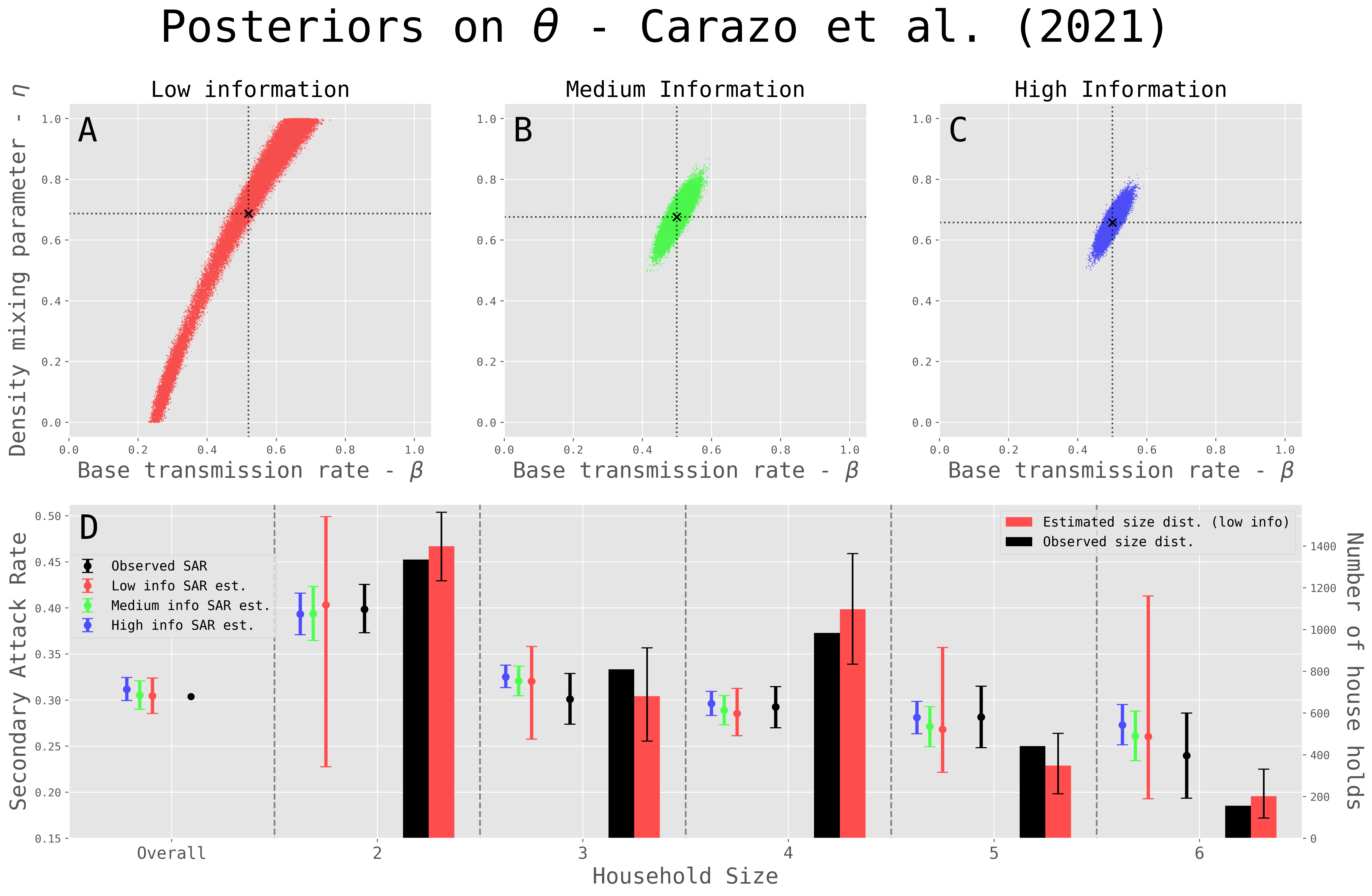
[8] reports final size data from outbreaks in households of health care workers in Québec, Canada during the COVID-19 pandemic. In that paper, final size data is reported in sufficient detail for a high information dataset. This allowed us to compare the performance of the MCMC method on a real dataset at each of the three information levels. For the choice of $\boldsymbol{\alpha}$ we used data from the 2021 Census in Canada which reported the number of households of each size in Québec. We use this distribution in the same way as the UK LFS (see Appendix C); however, given the census aggregated all households with 5 or more individuals, we arbitrarily distributed these households between sizes 5 and 6 at a 2:1 ratio. When estimating parameters, we used an $\boldsymbol{\alpha}$ centred around such a distribution, with a value of $\alpha_{0}=200$.

Figure 3: Panels A, B, and C show the posterior distributions of $\theta$ obtained by fitting the low- (red), medium- (green), and high-information (blue) versions of the data from [8], respectively. Panel D displays the secondary attack rate (SAR) implied by each posterior alongside the observed SAR (black) for each household size and overall; error bars represent 95% confidence intervals, with those for the observed SAR estimated by bootstrapping. Bars indicate the number of households of each size in the low-information fit (red) compared with the observed distribution (black). The infectious period is assumed to be $I\sim\text{Gamma}(2,2)$.

Panels A, B and C in Figure 3 show the posteriors of simultaneously fitting both $\beta$ and $\eta$ to the low- (red), medium- (green) and high-information datasets (blue). For each of these we had a $\text{Uniform}(0,1)$ prior on $\eta$ and an improper (positive reals) prior on $\beta$. These results are for $I\sim\text{Gamma}(2,2)$, though the same plots for $I\sim\text{Exponential}(1)$ and $I=1$ are shown in Figures S3 and S4 respectively. In Panel A of Figure 3 we can see that there were issues of identifiability between $\beta$ and $\eta$, with the MCMC exploring all values of $\eta$ (limited by assumption to [0,1]) and so we end up with a strip of values compatible with the observed SAR. With the medium-information dataset, instead, the parameters were clearly identifiable and the posterior was similar to, though slightly less certain than, the one obtained from the high-information dataset. The means in these two cases – shown by the black cross – are 0.57 (0.51, 0.63) for $\beta$ and 0.70 (0.59, 0.80) for $\eta$ for the medium-information dataset, and 0.57 (0.52, 0.62) for $\beta$ and 0.70 (0.61, 0.78) for $\eta$ for the high information one.

The error bars in Panel D of Figure 3 show the estimated overall and size-stratified SAR for each of the information levels and the observed values from [8]. The low-information confidence intervals do appear to cover the observed value for all sizes but are very wide, particularly for households of size 2 or 6. Adding higher levels of information incrementally narrows the confidence intervals and the medium- and high-information SAR estimates are close to those observed in the data. The bar chart in Panel D of Figure 3 shows the number of households of each size from the low information fit (red) and the observed data (black). The error bars cover the observed household size distribution showing that the algorithm proposed sensible household structures.

Next we estimated the transmission rate for SARS-CoV-2 from 23 papers [12, 27, 45, 17, 21, 43, 5, 18, 28, 13, 38, 40, 37, 44, 11, 19, 8, 30, 34] (25 datasets) that reported at least a low-information dataset. These were chosen from the ones considered by a series of literature reviews by Madewell et al. [22, 23, 24]. For each of these low information datasets we fit the base transmission rate ($\beta$) using the posterior for $\eta$ obtained from [8], combined with an improper prior on $\beta$, as the prior, i.e. $\pi(\theta)=\pi_{2}(\eta)$, and again assuming $I\sim\text{Gamma}(2,2)$. Using this prior was necessary given the issues with identifiability found for the low information case in Figure 3, but the resulting MCMC chains mixed well, as shown in the trace plots in Figures S5, S6 and S7.. For each study we found census or similar data to inform $\boldsymbol{\alpha}$ (in all cases, the data was size-weighted as discussed in Appendix C and we used $\alpha_{0}=200$). Each low information dataset and source for $\boldsymbol{\alpha}$ can be found in the supplementary CSV file. Figure 4 shows the estimates and 95% confidence intervals for each of these studies, split by variant – where specified – and colour coded accordingly. The table on the right hand size also shows the reported SAR, mean household size (including index cases) and number of households ($N$) for each study.

Figure 4: Base transmission rates ($\beta$) for SARS-CoV-2 estimated from low-information datasets from studies included in Madewell et al. [22, 23, 24], colour coded and grouped by strain where it was specified. A table on the right hand side lists the SAR, average household size and number of households in each of these studies.

We successfully inferred transmission parameters from low-information datasets, combining prior information on $\eta$ (in this case obtained from the high-information dataset in [8]) and information on the household size distribution of the relevant populations in $\boldsymbol{\alpha}$. We were able to properly account for differences in household size and better quantify the uncertainty compared to binomial confidence intervals often used for SARs.

Discussion

In this paper we present a novel MCMC algorithm for estimating epidemiological parameters from household final size data of different levels of coarseness. This includes very coarse “low information” datasets which only report the total number of household, total number of household contacts and total number of secondary cases. Without using an inference method to impute a household size distribution, like the MCMC approach we present here, it would not be possible to fit a mechanistic model to datasets of this kind. We first fit to low-information datasets derived from synthetically generated high-information dataset in order to assess the algorithm’s ability to recover the transmission rate, before applying the method to real data.

Insights

For data generated from a realistic household size distribution – in this paper, from the UK Labour Force Survey (UK LFS) – the algorithm reliably recovered the transmission rate $\beta$ for datasets generated from a range of parameter values of both $\beta$ and $\eta$. For all 12 parameter combinations we considered, the true value of $\beta$ was covered by the 95% confidence interval. However, the performance on data from an unrealistic “split” household size distribution, in which the majority of households had either 2 or 6 individuals (but the mean size of $\approx 3$ was the same), varied significantly for different parameters.

The performance was particularly poor in the case that $\alpha_{0}=100$ (relatively weak constraint on the household size distributions of a study from which a low-information dataset is collected). This is because the synthetic data was generated from the “split” household size distribution, but the MCMC was not strongly constrained to preserve that distribution and was settling on a distribution that include a significant number of households with sizes closer to the mean.

Given the strong non-linear relationship between the transmission rate and the SAR for different household sizes (see Figure S2), the same value of $\beta$ leads to a different SAR from the “split” distribution compared to the distribution the MCMC is settling on. In particular, for $\eta=0$ (bottom left panel of Figure S2), the former is larger than the latter, so to fit the same SAR, a significantly larger $\beta$ is required with the new distribution compared to the original one, causing the observed overestimation. This discrepancy is strongest for values of $\beta$ around 0.5, in line with what can be seen in Figure 2.

The same qualitative discrepancy is seen for $\eta=0.5$, though to a much less extent and reaching its maximum around 1.5, resulting in consistent overestimation for $\beta=1.5$ and $\beta=2.0$. The discrepancy, instead, is minimal for $\eta=1$, and interestingly is slightly reversed, which is compatible with the slight underestimation observed in this case in Figure 2.

Note that in all cases increasing the value of $\alpha_{0}$ constrained the MCMC to not drift away from the “split” distribution, leading to much better results, with a minimum of 93% of confidence intervals containing the actual values of $\beta$.

These results demonstrate the importance of the size distribution of the household study, which are often not reported in low-information datasets. In the absence of that information, assumptions need to be made about such a distribution and the confidence we have in it. However, such assumptions interact in non-trivial ways with the amount of person-to-person transmission and the assumed way in which transmission scales with the household size. However, although discrepancies emerge particularly strongly when mixing is close to being density-dependent ($\eta$ close to 0), for respiratory diseases such as SARS-CoV-2, which is the example used in this paper, it is common to assume frequency dependent mixing ($\eta=1$). In this case, estimates appear to be much less affected by deviations from the true distribution of the household size in the studies the low-information dataset comes from.

We then investigated the difference in performance when estimating both $\beta$ and $\eta$ simultaneously from low-, medium- and high-information datasets from [8]. The resulting posteriors on ($\beta,\eta$) demonstrate that at least medium-information datasets are necessary to confidently identify both simultaneously and that simply reporting low-information datasets is insufficient for transmission parameters to be estimated with any confidence in the absence of informative priors. However, if detailed data on the final size of outbreaks in each household cannot be reported in full, then total contacts and cases stratified by household size could still be used to identify both the transmission rate and the density mixing parameter almost to the same level of accuracy.

Finally, we estimated $\beta$ for a number of household studies which provided at least low-information datasets taken from the Madewell et al. systematic reviews [22, 23, 24]. Only 25 of the 144 studies included in these reviews a) tried to identify co-primary cases, b) dealt with suspected co-primaries in a way that preserved the household sizes and c) reported sufficient detail so that a low-information dataset could be extracted or derived.

Using existing inference methods, we would not be able to estimate transmission rates from these datasets. However, the framework presented in this paper allows us to consolidate these low-information final size datasets with household size data and prior information on the density mixing parameter to estimate transmission rates. Compared to the Binomial confidence intervals often used for estimates of SAR, the error bars in Figure 4 more accurately show the uncertainty in our estimates.

Limitations

In order to fit a transmission model to low-information data we were required to keep the model very simple. One limitation comes from our assumption of a single primary case. Many household studies limit the period of follow up in order to limit the risk of multiple independent introductions. However, multiple primary cases are not uncommon, e.g. when multiple residents attend social events together and so would be at risk of contracting a disease from a shared source.

One of the common uses of household-stratified transmission surveys is to estimate the relative susceptibility and infectivity associated with characteristics such as age, sex and ethnicity. In this work, however, we limited ourselves to identical individuals, all mixing homogeneously within each household, both to simplify the model for testing and to ensure that $g_{J}(D_{J})$ was not too large. However, future work could relax this assumption and perform a similar investigation to estimate the effects of risk factors on transmission.

Conclusion

In this paper we presented an MCMC algorithm that can estimate transmission rates from very coarse datasets of the type commonly reported in household transmission studies. We successfully recovered parameters from synthetic datasets and estimated transmission rates for COVID-19 under an assumption of frequency-dependent mixing from a number of household studies.

However, we also demonstrated that, in the absence of prior information on the parameter controlling how person-to-person transmission varies with household size, low information datasets are generally insufficient to resolve both this mixing parameter and the transmission rate. This result suggests researchers conducting household transmission studies can greatly improve the usefulness of their results for parametrising mechanistic models by reporting contacts and cases stratified by household size and, if possible, full information on the frequency of each outcome.

Code availability

All code used to implement the methods described in this paper and to generate all figures can be found in this GitHub repository.

Appendix A Formal Definitions of $g_{J}(D_{J})$

Medium-Information Datasets

Let a medium information dataset be encoded in a tuple of two vectors $D_{M}=(\mathbf{n},\mathbf{z})\in\mathbb{N}^{m}\times\mathbb{N}^{m}$ where $\mathbf{n}\geq\mathbf{z}$ element-wise. We can then define a function $g_{M}:\mathbb{N}^{m}\times\mathbb{N}^{m}\rightarrow\mathcal{P}(\mathbb{N}^{K})$ (where $\mathcal{P}(S)$ denotes the power set of of a set $S$) such that $g_{M}(D_{M})$ is the set of high information datasets compatible with the medium information dataset $D_{M}$. For the purpose of a formal definition of $g_{M}$ we define two matrices $\mathbf{A},\mathbf{B}\in\mathbb{N}^{m\times K}$ where

$$A_{i,k} =\begin{cases}i\quad\quad\quad\quad&\text{if }f(i,0)\leq k\leq f(i,i)\\ 0&\text{otherwise}\end{cases}$$ (14)

$$B_{i,k} =\begin{cases}k-f(i,0)&\>\text{if }f(i,0)\leq k\leq f(i,i)\\ 0&\>\text{otherwise}\end{cases}$$ (15)

Then

$$g_{M}((\mathbf{n},\mathbf{z}))=\{\mathbf{C}\in\mathbb{N}^{K}:(\mathbf{AC}=\mathbf{n})\>\land\>(\mathbf{BC}=\mathbf{z})\}$$ (16)

Similar to the high-information case, since $\sum_{k=f(n,0)}^{f(n,n)}C_{k}$ is the same for all $n=1,\dots,m$ and $\mathbf{C}\in g_{M}((\mathbf{n},\mathbf{z}))$ the choice of $\boldsymbol{\alpha}$ does not effect the likelihood.

Low-information Datasets

Let a low-information dataset be encoded by three integers in a 3-tuple, denoted $D_{L}=(N,n,z)\in\mathbb{N}^{3}$ where $z\leq n$ and $N\leq n\leq mN$. $N$ denotes the number of households, $n$ the total number of contacts and $z$ the total number of cases. We can then again define a function $g_{L}:\mathbb{N}^{3}\rightarrow\mathcal{P}(\mathbb{N}^{K})$ where $g_{L}(D_{L})$ is the set of high information datasets compatible with the low information datasets. For low information datasets we will define $g_{L}(D_{L})$ similarly to how we did for $g_{M}(D_{M})$. We define two vectors, $\mathbf{w}$ and $\mathbf{v}\in\mathbb{N}^{K}$, such that $w_{k}=f_{n}(k)$ and $v_{k}=f_{z}(k)$ and so

$$g_{L}((N,n,z))=\{\mathbf{C}\in\mathbb{N}^{K}:(\langle\mathbf{C},\mathbf{w}\rangle=n)\>\land\>(\langle\mathbf{C},\mathbf{v}\rangle=z)\>\land\>(\langle\mathbf{C},\mathbf{1}\rangle=N)\}$$ (17)

Appendix B Proposal algorithms for $q_{M}$ and $q_{L}$

Algorithm 1 Low information new frequency count pseudo-dataset proposal algorithm

1:$\mathbf{C}=(C_{0},\dots,C_{K})\in\mathbf{N}^{K-1}$

2:Calculate the total number of households with at least 2 contacts,

$$S_{1}=\sum_{\{k:f_{n}(k)\geq 2\}}C_{k}.$$

3:Calculate a probability distribution proportional to the number of households with each outcome and conditioned on there being at least 2 contacts $P_{1}=(0,0,\frac{C_{2}}{S_{1}},\dots,\frac{C_{K}}{S_{1}})$

4:Sample an index $k_{1}$ from $P_{1}$ and denote $f_{n}(k_{1})$ and $f_{z}(k_{1})$ by $n_{1}$ and $z_{1}$ respectively.

5:Uniformly draw a random number $u_{\text{inf}}\in[0,1]$

6:if $u_{\text{inf}}\leq\frac{z_{1}}{n_{1}}$ then an infected contact is chosen and we set $s=1$ else set $s=0$

7:Calculate the total number of households with fewer than $m$ contacts,

$$S_{2}=\sum_{\{k:f_{n}(k)\leq(m-1)\}}c_{k}$$

8:Calculate another probability vector $P_{2}$ conditioned on there being fewer than the maximum number of contacts such that for $k=0,\dots,K$:

$$P_{2k}=\begin{cases}\frac{c_{k}}{S_{2}-1}&\text{ if }f_{n}(k)<m\text{ and }k\neq k_{1}\\ \frac{c_{k}-1}{S_{2}-1}&\text{ if }k=k_{1}\\ 0&\text{ otherwise}\end{cases}$$ (18)

9:Draw a second index, $k_{2}$, from $P_{2}$ and denote $f_{n}(k_{2})$ and $f_{z}(k_{2})$ by $n_{2}$ and $z_{2}$ respectively.

10:Define a new frequency count partition $C^{*}=(c_{0}^{*},\dots,c_{K}^{*})$ by starting with a copy of the original frequency count partition, $\mathcal{C}$.

11:Update the entries $c_{k_{1}}^{*}$ and $c_{k_{2}}^{*}$ in turn by subtracting 1. Note it could be that $k_{1}=k_{2}$ in which case we subtract 2 from $c_{k_{1}}^{*}$ in this step.

12:Define

$$k_{3}=f(n_{1}-1,z_{1}-s)\text{ and }k_{4}=f(n_{2}+1,z_{2}+s).$$

13:Update the entries $c_{k_{3}}^{*}$ and $c_{k_{4}}^{*}$ in turn by adding 1. Note that it is possible that $k_{3}=k_{2}$ and/or $k_{4}=k_{1}$ and the entries at those indices are unchanged.

Algorithm 2 Medium information new partition proposal algorithm

1:$C=(c_{0},\dots,c_{K})$

2:Calculate the total number of cases in households with at least 2 contacts, $S_{1}=\sum_{k=2}^{K}c_{k}f_{z}(k)$

3:Calculate a probability distribution proportional to the number of households with each outcome and conditioned on there being at least 2 contacts

$$P_{1}=(0,0,0,\frac{c_{3}}{S_{1}},\frac{2c_{4}}{S_{1}},\dots,\frac{mc_{K}}{S_{1}})$$

4:Sample an index $k_{1}$ from $P_{1}$. Denote $f_{n}(k_{1})$ and $f_{z}(k_{1})$ by $n_{1}$ and $z_{1}$ respectively.

5:Calculate the number of non-case contacts in households with $n_{1}$ contacts

$$S_{2}=\sum_{k=f(n_{1},0)}^{f(n_{1},n_{1})}(n_{1}-f_{z}(k))c_{k}$$

6:Calculate another probability vector $P_{2}$ conditioned on their being $n_{1}$ contacts and weighted by the number of non-case contacts. For $k=0,\dots,K$:

$$P_{2k}=\begin{cases}\frac{c_{k}(n_{1}-f_{z}(k))}{S_{2}-1}&\text{ if }f_{n}(k)=n_{1}\text{ and }k\neq k_{1}\\ \frac{(c_{k}-1)(n_{1}-f_{z}(k))}{S_{2}-1}&\text{ if }k=k_{1}\\ 0&\text{ otherwise}\end{cases}$$ (19)

7:Draw a second index, $k_{2}$, from $P_{2}$

8:Define a new frequency count partition $C^{*}=(c_{0}^{*},\dots,c_{K}^{*})$ by starting with a copy of the original frequency count partition, $\mathcal{C}$.

9:Update the entries $c_{k_{1}}^{*}$ and $c_{k_{2}}^{*}$ in turn by subtracting 1. Note it could be that $k_{1}=k_{2}$ in which case we subtract 2 from $c_{k_{1}}^{*}$ in this step.

10:Update the entries $c_{k_{1}-1}^{*}$ and $c_{k_{2}+1}^{*}$ in turn by adding 1.

Appendix C Household size distributions

We generated synthetic data for two very different household distributions: the UK Labour Force Survey (LFS) from 2023 and an unrealistic “split” distribution in which most households are either composed of 2 or the maximum (6) number of individuals. In the former case, we took the UK LFS household size distribution, removed the probability of selecting a household of size 1 and re-normalised the distribution, obtaining the probability $P_{\text{UK}}^{k}$ that a randomly selected household in our population is of size $k$ ($k=2,\dots,6$). We then derived the size-weighted distribution, i.e. we made the probability of a household included dataset having $k$ contacts proportional to $kP_{UK}^{k}$. This is the household distribution we would expect to see in our study if an infection spreading between household could be described well by a homogeneously mixing model in the general population, so that each individual in the population is equally likely be infected, and further assuming the same probability for each case to be detected and have their household included in the study. The split distribution was selected so that the mean of the size-weighted distribution was the same as the size-weighted distribution based on the UK LFS. See Figure S1 for the size-weighted distributions used.

Appendix D Procedure for selecting appropriate papers from [24]

From the full list of papers that estimated secondary attack rate in [24], we first filtered out papers, so that the remaining ones were compatible with the model assumptions and that we could extract a low-information dataset, according to the following criteria:

1. In each household, all contacts must have been tested or screened for symptoms;

2. There was a procedure for identifying the primary and co-primary cases, e.g. based on symptom onset or epidemiological investigation;

3. If co-primary cases were suspected, those individuals were not removed without the rest of the household being removed, as this would have left the household partially depleted;

4. There was sufficient information reported to deduce a total number of contacts, cases and households.

Papers that received ad-hoc consideration were the following:

• [17]: SAR was reported for family clusters, not households. Here, the work was included, with clusters treated as households.

• [36]: SARs were reported for 127 households and 138 index cases. It was not possible to disentangle the contacts in households with a single primary cases from the information provided and so this paper was not included.

• [11]: Different SARs, based on PCR testing and symptoms, were reported. We included the data from PCR testing.

• [39]: The number of households with a single primary case in the study was not clear and so this paper was not included.

• [32]: The number of households was not explicitly stated and so was estimated from the mean household size and total number of contacts as $225/2.3\approx 98$ households. The paper was included.

Supplementary plots

Figure S1: Size-weighted household size distributions that were used to generate synthetic data. The distribution for the UK LFS (2023) [31] and the “split” distribution are shown in red and blue, respectively. Both distributions share a mean final size, after size weighting, of 3.32 which is shown by the vertical black dotted line. For the purpose of this paper households reported to have 6+ individuals in the UK LFS are assumed to have size exactly 6.

	$\beta=0.2$		$\beta=0.5$		$\beta=1.5$
	UK	Split	UK	Split	UK	Split
$\eta=0$	22.2(19.9,24.1)%	25.3(22.4,27.9)%	50.2(47.3,52.7)%	56.9(54.1,60.0)%	84.1(81.9,86.2)%	86.7(84.6,88.4)%
$\eta=0.5$	13.2(11.7,14.6)%	13.3(11.9,14.9)%	32.6(29.9,34.7)%	33.4(31.0,36.2)%	71.6(68.6,73.9)%	74.3(71.6,76.8)%
$\eta=1$	8.6(7.3,10.0)%	8.2(7.0,9.4)%	21.0(19.3,22.9)%	19.6(17.6,21.5)%	52.5(49.8,55.1)%	50.8(47.5,54.4)%
	$\beta=2.0$
	UK	Split
$\eta=0$	80.3(77.6,82.6)%	90.5(88.8,91.9)%
$\eta=0.5$	80.3(77.6,82.6)%	82.5(80.1,85.0)%
$\eta=1$	63.3(60.7,66.5)%	62.1(59.0,66.0)%

Table S1: The secondary attack rates (SAR) from the synthetic datasets for each value of $\beta$, $\eta$ and household size distribution. These results are obtained for an infectious period distribution $I\sim\text{Gamma}(2,2)$.

Figure S2: In this figure we compare the mean final size (top row) and mean SAR (bottom row) for households of different sizes (2–6) for different transmission rates ($\beta$ – shown on the x-axis). Vertical dashed lines are shown at the values of $\beta$ considered in Figure 2. Each row shows results for a different value of $\eta$, ranging from $\eta=0$ (density dependent mixing), $\eta=0.5$ and $\eta=1$ (frequency dependent mixing). We also show the mean final size/SAR for two different household size distributions: the “split” distribution shown in Figure S1 and the household size distribution that the MCMC chain resulting from the data augmentation process from the low-information data settles on: this was derived by averaging over the chains obtained from fitting the datasets generated from $\eta=1$, $\beta=0.5$, the “split” distribution and $\alpha_{0}=100$. This mean household size distribution is similar for other values of $\eta$ and $\beta$.

Figure S3: Panels A, B, and C show the posterior distributions of $\theta$ obtained by fitting the low- (red), medium- (green), and high-information (blue) versions of the data from [8], respectively. Panel D displays the secondary attack rate (SAR) implied by each posterior alongside the observed SAR (black) for each household size and overall; error bars represent 95% confidence intervals, with those for the observed SAR estimated by bootstrapping. Bars indicate the number of households of each size in the low-information fit (red) compared with the observed distribution (black). The infectious period is assumed to be $I\sim\text{Exponential}(1)$.

Figure S4: Panels A, B, and C show the posterior distributions of $\theta$ obtained by fitting the low- (red), medium- (green), and high-information (blue) versions of the data from [8], respectively. Panel D displays the secondary attack rate (SAR) implied by each posterior alongside the observed SAR (black) for each household size and overall; error bars represent 95% confidence intervals, with those for the observed SAR estimated by bootstrapping. Bars indicate the number of households of each size in the low-information fit (red) compared with the observed distribution (black). The infectious period is assumed to be fixed to $I=1$.

Figure S5: Trace plots for $\beta$ for each of the papers reporting low information datasets taken from Madewell et al. (datasets 1-10). Each plot is colour-coded by the variant, as in Figure 4: blue for pre-Alpha, green for Alpha, orange for Delta, red for Omicron and black for Unspecified/Other. Note that the chain lengths ($x$-axis ranges) vary significantly between panels and that all chains mix well: those that appear not to mix well are just much shorter than the others and correspond to studies with small numbers of households.

Figure S6: Trace plots for $\beta$ for each of the papers reporting low information datasets taken from Madewell et al. (datasets 11-20). Each plot is colour-coded by the variant, as in Figure 4: blue for pre-Alpha, green for Alpha, orange for Delta, red for Omicron and black for Unspecified/Other. Note that the chain lengths ($x$-axis ranges) vary significantly between panels and that all chains mix well: those that appear not to mix well are just much shorter than the others and correspond to studies with small numbers of households.

Figure S7: Trace plots for $\beta$ for each of the papers reporting low information datasets taken from Madewell et al. (datasets 21-28). Each plot is colour-coded by the variant, as in Figure 4: blue for pre-Alpha, green for Alpha, orange for Delta, red for Omicron and black for Unspecified/Other. Note that the chain lengths ($x$-axis ranges) vary significantly between panels and that all chains mix well: those that appear not to mix well are just much shorter than the others and correspond to studies with small numbers of households.

References

- [1] The final size distribution for a generalized stochastic epidemic. Ph.D., Emory University, United States – Georgia, (English). External Links: ISBN 979-8-206-78084-0, Link Cited by: Introduction.
- [2] (1995) A Generalized Model of Parasitoid, Venereal, and Vector-Based Transmission Processes. The American Naturalist 145 (5), pp. 661–675. External Links: ISSN 0003-0147, Link Cited by: Transmission model.
- [3] (2021) Risk Factors, Epidemiological and Clinical Outcome of Close Contacts of COVID-19 Cases in a Tertiary Hospital in Southern India. JOURNAL OF CLINICAL AND DIAGNOSTIC RESEARCH (en). External Links: ISSN 2249782X, Link, Document Cited by: Introduction.
- [4] (2021-03) A case-control study of determinants for COVID-19 infection based on contact tracing in Dungun district, Terengganu state of Malaysia. Infectious Diseases (London, England) 53 (3), pp. 222–225 (eng). External Links: ISSN 2374-4243, Document Cited by: Introduction.
- [5] (2022-03) SARS-CoV-2 B.1.1.529 (Omicron) Variant Transmission Within Households — Four U.S. Jurisdictions, November 2021–February 2022. Morbidity and Mortality Weekly Report 71 (9), pp. 341–346. External Links: ISSN 0149-2195, Link, Document Cited by: Fitting to real data.
- [6] (2016-04) Reproduction numbers for epidemic models with households and other social structures II: Comparisons and implications for vaccination. Mathematical Biosciences 274, pp. 108–139. External Links: ISSN 0025-5564, Link, Document Cited by: Introduction.
- [7] (1986) A Unified Approach to the Distribution of Total Size and Total Area under the Trajectory of Infectives in Epidemic Models. Advances in Applied Probability 18 (2), pp. 289–310. External Links: ISSN 0001-8678, Link, Document Cited by: Likelihood.
- [8] (2021-04) Characterization and evolution of infection control practices among severe acute respiratory coronavirus virus 2 (SARS-CoV-2)–infected healthcare workers in acute-care hospitals and long-term care facilities in Québec, Canada, Spring 2020. Infection Control & Hospital Epidemiology 43 (4), pp. 481–489 (en). External Links: ISSN 0899-823X, 1559-6834, Link, Document Cited by: Figure S3, Figure S4, Introduction, Figure 3, Fitting to real data, Fitting to real data, Fitting to real data, Fitting to real data, Insights.
- [9] (2004) A Bayesian MCMC approach to study transmission of influenza: application to household longitudinal data. Statistics in Medicine 23 (22), pp. 3469–3487 (en). Note: _eprint: https://onlinelibrary.wiley.com/doi/pdf/10.1002/sim.1912 External Links: ISSN 1097-0258, Link, Document Cited by: Transmission model.
- [10] (1995) How Does Transmission of Infection Depend on Population Size?. In Epidemic models: their structure and relation to data, pp. 84–94. Cited by: Transmission model.
- [11] (2022) High secondary attack rate and persistence of SARS-CoV-2 antibodies in household transmission study participants, Finland 2020-2021. Frontiers in Medicine 9, pp. 876532 (eng). External Links: ISSN 2296-858X, Document Cited by: 3rd item, Fitting to real data.
- [12] (2021-03) Incidence, household transmission, and neutralizing antibody seroprevalence of Coronavirus Disease 2019 in Egypt: Results of a community-based cohort. PLOS Pathogens 17 (3), pp. e1009413 (en). External Links: ISSN 1553-7374, Link, Document Cited by: Fitting to real data.
- [13] (2022-08) Increased transmissibility of SARS-CoV-2 alpha variant (B.1.1.7) in children: three large primary school outbreaks revealed by whole genome sequencing in the Netherlands. BMC infectious diseases 22 (1), pp. 713 (eng). External Links: ISSN 1471-2334, Document Cited by: Fitting to real data.
- [14] (2022-09) A computational framework for modelling infectious disease policy based on age and household structure with applications to the COVID-19 pandemic. PLOS Computational Biology 18 (9), pp. 1–38. External Links: Link, Document Cited by: Introduction.
- [15] (2022-09) Inferring risks of coronavirus transmission from community household data. Statistical Methods in Medical Research 31 (9), pp. 1738–1756 (en). External Links: ISSN 0962-2802, Link, Document Cited by: Introduction.
- [16] (2013-02) How big is an outbreak likely to be? Methods for epidemic final-size calculation. Proceedings of the Royal Society A: Mathematical, Physical and Engineering Sciences 469 (2150), pp. 20120436. External Links: Link, Document Cited by: Likelihood.
- [17] (2021-06) Household transmission but without the community-acquired outbreak of COVID-19 in Taiwan. Journal of the Formosan Medical Association 120, pp. S38–S45. External Links: ISSN 0929-6646, Link, Document Cited by: 1st item, Fitting to real data.
- [18] (2022-02) Increased household transmission and immune escape of the SARS-CoV-2 Omicron variant compared to the Delta variant: evidence from Norwegian contact tracing and vaccination data. medRxiv (en). Note: Pages: 2022.02.07.22270437 External Links: Link, Document Cited by: Fitting to real data.
- [19] (2021-04) Transmission of COVID-19 and its Determinants among Close Contacts of COVID-19 Patients Running title. Journal of Research in Health Sciences 21 (2), pp. e00514 (eng). External Links: ISSN 2228-7809, Document Cited by: Fitting to real data.
- [20] (2009-09) Bayesian analysis for emerging infectious diseases. Bayesian Analysis 4 (3), pp. 465–496 (en). External Links: ISSN 1936-0975, 1931-6690, Link, Document Cited by: Introduction.
- [21] (2020-08) Household Transmission of SARS-CoV-2 in the United States. Clinical Infectious Diseases: An Official Publication of the Infectious Diseases Society of America, pp. ciaa1166. External Links: ISSN 1058-4838, Link, Document Cited by: Fitting to real data.
- [22] (2020-12) Household Transmission of SARS-CoV-2: A Systematic Review and Meta-analysis. JAMA Network Open 3 (12), pp. e2031756. External Links: ISSN 2574-3805, Link, Document Cited by: Figure 4, Fitting to real data, Insights.
- [23] (2021-08) Factors Associated With Household Transmission of SARS-CoV-2: An Updated Systematic Review and Meta-analysis. JAMA Network Open 4 (8), pp. e2122240. External Links: ISSN 2574-3805, Link, Document Cited by: Figure 4, Fitting to real data, Insights.
- [24] (2022-04) Household Secondary Attack Rates of SARS-CoV-2 by Variant and Vaccination Status: An Updated Systematic Review and Meta-analysis. JAMA Network Open 5 (4), pp. e229317. External Links: ISSN 2574-3805, Link, Document Cited by: Appendix D, Appendix D, Introduction, Introduction, Figure 4, Fitting to real data, Insights.
- [25] (2001-06) How should pathogen transmission be modelled?. Trends in Ecology & Evolution 16 (6), pp. 295–300 (English). External Links: ISSN 0169-5347, Link, Document Cited by: Transmission model.
- [26] (2008) Social contacts and mixing patterns relevant to the spread of infectious diseases. PLoS medicine 5 (3), pp. e74. Cited by: Introduction.
- [27] (2022-05) Risk factors associated with household transmission of SARS-CoV-2 in Negeri Sembilan, Malaysia. Journal of Paediatrics and Child Health 58 (5), pp. 769–773 (eng). External Links: ISSN 1440-1754, Document Cited by: Fitting to real data.
- [28] (2022-07) Impact of Severe Acute Respiratory Syndrome Coronavirus 2 (SARS-CoV-2) Vaccination and Pediatric Age on Delta Variant Household Transmission. Clinical Infectious Diseases 75 (1), pp. e35–e43. External Links: ISSN 1058-4838, Link, Document Cited by: Fitting to real data.
- [29] (1999-01) Bayesian Inference for Partially Observed Stochastic Epidemics. Journal of the Royal Statistical Society Series A: Statistics in Society 162 (1), pp. 121–129. External Links: ISSN 0964-1998, Link, Document Cited by: Introduction.
- [30] (2022-01) Increased Secondary Attack Rates among the Household Contacts of Patients with the Omicron Variant of the Coronavirus Disease 2019 in Japan. International Journal of Environmental Research and Public Health 19 (13), pp. 8068 (en). Note: Number: 13 External Links: ISSN 1660-4601, Link, Document Cited by: Fitting to real data.
- [31] (2024-05) Families and households statistics explained - Office for National Statistics. External Links: Link Cited by: Figure S1, Introduction, Synthetic data generation.
- [32] (2020-08) Coronavirus Disease Outbreak in Call Center, South Korea. Emerging Infectious Diseases 26 (8), pp. 1666–1670. External Links: ISSN 1080-6040, Link, Document Cited by: 5th item.
- [33] (2011-10) Epidemic growth rate and household reproduction number in communities of households, schools and workplaces. Journal of Mathematical Biology 63 (4), pp. 691–734 (en). External Links: ISSN 1432-1416, Link, Document Cited by: Introduction.
- [34] (2021-12) Risk of Secondary Household Transmission of COVID-19 from Health Care Workers in a Hospital in Spain. Epidemiologia (Basel, Switzerland) 3 (1), pp. 1–10 (eng). External Links: ISSN 2673-3986, Document Cited by: Fitting to real data.
- [35] (2008-11) Contact rate calculation for a basic epidemic model. Mathematical Biosciences 216 (1), pp. 56–62. External Links: ISSN 0025-5564, Link, Document Cited by: Transmission model.
- [36] (2022-02) Community transmission and viral load kinetics of the SARS-CoV-2 delta (B.1.617.2) variant in vaccinated and unvaccinated individuals in the UK: a prospective, longitudinal, cohort study. The Lancet Infectious Diseases 22 (2), pp. 183–195 (English). External Links: ISSN 1473-3099, 1474-4457, Link, Document Cited by: 2nd item.
- [37] (2021-03) Low secondary transmission rates of SARS-CoV-2 infection among contacts of construction laborers at open air environment. Germs 11 (1), pp. 128–131 (eng). External Links: ISSN 2248-2997, Document Cited by: Fitting to real data.
- [38] (2021-07) Increased Transmissibility of the SARS-CoV-2 Alpha Variant in a Japanese Population. International Journal of Environmental Research and Public Health 18 (15), pp. 7752 (eng). External Links: ISSN 1660-4601, Document Cited by: Fitting to real data.
- [39] (2022) SARS-CoV-2 Transmission Dynamics in Households With Children, Los Angeles, California. Frontiers in Pediatrics 9. External Links: ISSN 2296-2360, Link Cited by: 4th item.
- [40] (2020-11) Burden of Illness in Households With Severe Acute Respiratory Syndrome Coronavirus 2–Infected Children. Journal of the Pediatric Infectious Diseases Society 9 (5), pp. 613–616. External Links: ISSN 2048-7207, Link, Document Cited by: Fitting to real data.
- [41] (2020-12) Bayesian inference for multistrain epidemics with application to ESCHERICHIA COLI O157:H7 in feedlot cattle. The Annals of Applied Statistics 14 (4), pp. 1925–1944. External Links: ISSN 1932-6157, 1941-7330, Link, Document Cited by: Introduction.
- [42] (2022-04) Differences in Transmission between SARS-CoV-2 Alpha (B.1.1.7) and Delta (B.1.617.2) Variants. Microbiology Spectrum 10 (2), pp. e00008–22. External Links: Link, Document Cited by: Introduction.
- [43] (2022-05) Transmission of SARS-CoV-2 within households: a remote prospective cohort study in European countries. European Journal of Epidemiology 37 (5), pp. 549–561 (en). External Links: ISSN 1573-7284, Link, Document Cited by: Fitting to real data.
- [44] (2020-07) Basic epidemiological parameter values from data of real-world in mega-cities: the characteristics of COVID-19 in Beijing, China. BMC Infectious Diseases 20 (1), pp. 526. External Links: ISSN 1471-2334, Link, Document Cited by: Fitting to real data.
- [45] (2021-12) Transmissibility of SARS-CoV-2 Variants as a Secondary Attack in Thai Households: a Retrospective Study. IJID regions 1, pp. 1–2 (eng). External Links: ISSN 2772-7076, Document Cited by: Fitting to real data.
- [46] (2016-03) Reconstructing transmission trees for communicable diseases using densely sampled genetic data. The Annals of Applied Statistics 10 (1), pp. 395–417 (en). External Links: ISSN 1932-6157, 1941-7330, Link, Document Cited by: Introduction.