Lagrangian Relaxation Score-based Generation for
Mixed Integer linear Programming

Abstract

Predict-and-search (PaS) methods have shown promise for accelerating mixed-integer linear programming (MILP) solving. However, existing approaches typically assume variable independence and rely on deterministic single-point predictions, which limits solution diversity and often necessitates extensive downstream search for high-quality solutions. In this paper, we propose SRG, a generative framework based on Lagrangian relaxation-guided stochastic differential equations (SDEs), with theoretical guarantees on solution quality. SRG leverages convolutional kernels to capture inter-variable dependencies while integrating Lagrangian relaxation to guide the sampling process toward feasible and near-optimal regions. Rather than producing a single estimate, SRG generates diverse, high-quality solution candidates that collectively define compact and effective trust-region subproblems for standard MILP solvers. Across multiple public benchmarks, SRG consistently outperforms existing machine learning baselines in solution quality. Moreover, SRG demonstrates strong zero-shot transferability: on unseen cross-scale/problem instances, it achieves competitive optimality with state-of-the-art exact solvers while significantly reducing computational overhead through faster search and superior solution quality.

1 Introduction

Mixed Integer Linear Programming (MILP) can formulate a wide range of combinatorial optimization problems, many of which are NP-hard (Karp, 1972). MILP has been widely applied in production planning (Ye et al., 2023), resource allocation (Ejaz and Choudhury, 2025), and energy management (Pinzon et al., 2017), as well as in emerging applications across advanced manufacturing. However, due to the inherent NP-hardness of MILP, finding provably optimal solutions is computationally intractable for large instances. Although exact algorithms such as Branch and Bound and Cutting-Plane methods (Gomory, 1958) provide optimality guarantees, they often incur prohibitive computational costs on large instances, limiting their practicality in time-sensitive real-world applications (Bengio et al., 2020).

Recently, machine learning has shown great potential in accelerating MILP solving by leveraging structural similarities across problem instances and reusing decision knowledge (Gasse et al., 2019; Gupta et al., 2020; Ling et al., 2024). Among these approaches, Predict-and-Search (PaS) has emerged as a particularly effective paradigm (Han et al., 2023; Geng et al., 2025; Liu et al., 2025), which can significantly reduce the runtime of traditional MILP solvers. Specifically, PaS methods employ Graph Neural Networks (GNNs) over bipartite variable-constraint graphs to estimate the marginal probabilities of variable assignments, thereby identifying promising subspaces or critical structures where high-quality solutions are likely to reside. A conventional exact MILP solver (i.e. SCIP & Gurobi) is then invoked to search within these reduced regions to efficiently find near-optimal solutions.

Despite their success, existing PaS frameworks exhibit fundamental limitations. Their predictive models inherently rely on imitating labels without explicitly enforcing global feasibility or optimality conditions. Furthermore, by predicting variables in isolation rather than modeling their joint dependencies, these models struggle to respect the complex coupling constraints inherent in MILP (Wolsey and Nemhauser, 1999). Consequently, the raw predictions may lack structural validity, resulting in imprecise trust regions (Han et al., 2023), which can increase computational overhead and degrade solution quality in the subsequent search phase.

Figure 1: Generation trajectory of our method on a 2D Linear Programming toy experiment (a special case of MILP). As the denoising process evolves, the learned score density (yellow heatmap) progressively concentrates toward the optimal solution (red star), effectively steering the samples (blue dots) from an initially scattered state into a tight cluster near the optimum. Additional experiment details are provided in Appx. B.

Motivated by these limitations, we propose a novel framework that moves beyond purely supervised prediction by explicitly incorporating feasibility and optimality into the solution generation process. Our core contribution lies in formulating the training objective with Lagrangian relaxations, which explicitly penalizes constraint violations and suboptimality. We theoretically demonstrate that optimizing this regularized objective is mathematically equivalent to aligning the generative process with a refined target distribution, where probability mass is exponentially re-weighted towards feasible and high-quality regions. This formulation naturally motivates the use of a guided reverse-time Stochastic Differential Equation (SDE) (Song et al., 2021; Karras et al., 2024). This choice is both principled and effective. Theoretically, the SDE is constructed such that its stationary distribution converges to the refined target, while its iterative denoising process provides a direct mechanism to incorporate gradient guidance from constraint and objective terms. Starting from a Gaussian distribution, the model progressively denoises toward feasible and high-quality regions (Figure 1). Crucially, this SDE-based formulation enables joint modeling of all decision variables, overcoming the independence assumptions of marginal-based predictions. Furthermore, once trained, the sampler can generate multiple diverse solution candidates via repeated sampling, substantially improving robustness over conventional single-shot predictions. Overall, our generative framework encourages structurally valid solutions and minimizes search effort, while its joint modeling and diverse sampling capabilities provide a robust foundation for efficient MILP solving. Our key contributions are as follows:

1) We show that optimizing Lagrangian-relaxation objective in probabilistic modeling is theoretically equivalent to learning a refined target distribution, forming a principled basis for feasibility- and optimality-aware generation.
2) We propose a guided reverse-time SDE sampler that jointly generates all decision variables, addressing independence issues inherent in marginal-based predictions.
3) We enable diverse candidate generation via parallel sampling from a Gaussian distribution to a Lagrangian-relaxation guided distribution, improving robustness over conventional single-shot predictions.

2 Related Work

Mixed Integer Linear Programming (MILP) problems rank among the most challenging combinatorial optimization tasks due to their hybrid decision spaces involving both continuous and discrete variables. Exact solvers, such as branch-and-bound and cutting-plane algorithms (Land and Doig, 1960), solve MILPs with guaranteed solution optimality by MILP problem reduction. In recent years, machine learning-based methods have emerged as a promising direction for accelerating MILP solving. Diffusion model based solvers that exploit specific structural properties of MILP instances (e.g., TSP problems with Hamiltonian cycles) (Sun and Yang, 2023), Predict-and-Search (PaS) frameworks (Han et al., 2023; Huang et al., 2024) has effectively solved the MILPs by construction powerful solutions. Among these, PaS and its downstream methods have proven particularly effective by learning the marginal distributions of end-to-end solutions to construct high-quality search regions, thereby significantly improving solver efficiency for large-scale MILPs.

3 Preliminaries

Mixed Integer Linear Programming (MILP) optimizes a linear objective subject to linear constraints and integrality restrictions. For an instance with $m$ constraints and $n$ variables, the standard MILP formulation is:

where $A\in\mathbb{R}^{m\times n}$, $c^{T}\in\mathbb{R}^{n}$, $b\in\mathbb{R}^{m}$, $l,u\in(\mathbb{R}\cup\{\pm/\})^{n}$, and $I\subseteq\{1,\dots,n\}$ denotes the set of indices for integer-constrained variables. The feasible region is:

MILP Bipartite Graph Representation. Following Gasse et al. (2019), any MILP instance $(A,b,c)$ can be represented as a bipartite graph $\mathcal{G}=(\mathcal{V},\mathcal{C},\mathcal{E})$, where $\mathcal{V}$ and $\mathcal{C}$ denote variable and constraint nodes, respectively. This graph is then encoded into an embedding $\mathbf{g}=\tau_{\phi}(A,b,c)$ via a 2-layer GNN encoder $\tau_{\phi}$, which captures variable–constraint interactions in a compact form. The embedding $\mathbf{g}$ is then used as the structural conditioning input for downstream learning modules.

Lagrangian Relaxation. For the MILP in Eq. (1) with optimal value $z^{*}_{\text{MILP}}$, suppose the constraints are partitioned into “complicating” constraints $Ax\geq b$ and “easy” constraints $x\in X$ (e.g., integrality and bound constraints). The Lagrangian relaxation dualizes the complicating constraints with multipliers:

$$L(\lambda)=\min_{x\in X}\left\{cx+\lambda^{\top}(b-Ax)\right\}.$$ (2)

It is well-established that for any $\lambda_{i}\geq 0(i=1,2,...,m)$, $L(\lambda)\leq z^{*}_{\text{MILP}}$, providing a valid lower bound.

Theorem 1 (Subgradient Convergence (Shor, 1985)).

Consider the Lagrangian dual problem:

$$z_{\text{LD}}=\max_{\lambda\geq 0}L(\lambda).$$ (3)

Let $\{\lambda_{(k)}\}$ be the sequence of multipliers generated by the subgradient method:

$$\lambda_{(k+1)}=\max\left(0,\lambda_{(k)}+\alpha_{k}(b-Ax_{(k)})\right),$$ (4)

where $x_{(k)}\in\arg\min_{x\in X}\{cx+(\lambda_{(k)})^{\top}(b-Ax)\}$, and the step sizes $\{\alpha_{k}\}$ satisfy:

$$\alpha_{k}>0,\quad\sum_{k=1}^{\infty}\alpha_{k}=\infty,\quad\sum_{k=1}^{\infty}\alpha_{k}^{2}<\infty.$$ (5)

Then the sequence of dual values converges to the optimal dual value:

$$\lim_{k\to\infty}L(\lambda_{(k)})=z_{\text{LD}}\leq z_{\text{MILP}}^{*}.$$ (6)

The Lagrangian relaxation solution $x^{*}(\lambda)$ preserves the combinatorial structure of the original MILP while relaxing complicating constraints. It provides valuable structural information that can guide the search process by identifying promising regions in the solution space (Fisher, 1981).

4 Our Method

We propose SRG (Score-based generative framework with Lagrangian Relaxation Guidance), which formulates MILP solution prediction as sampling from a refined target distribution. The framework consists of two core components: (1) Target Formulation, which incorporates Lagrangian relaxation to construct a probability density that concentrates mass on feasible and high-quality solutions; and (2) Guided Sampling, which samples from this target distribution via a reverse-time SDE. By injecting gradients derived from feasibility and objective-quality terms into the denoising dynamics, SRG captures joint dependencies among variables while steering generation toward desirable solution regions.

4.1 Lagrangian Relaxation-guided SDEs

Leveraging the bipartite graph embedding $\mathbf{g}$ as the structural condition, we formulate MILP solution prediction as a conditional generative task. Our goal is to learn a parameterized distribution $q_{\theta}(x|\mathbf{g})$ that approximates the target distribution of optimal solutions $p(x^{*}|\mathbf{g})$. Unlike deterministic approaches that output a single prediction, this probabilistic formulation enables sampling of diverse candidate solutions from the learned distribution, thereby increasing the likelihood of finding high-quality solutions. A standard approach to achieve this is to minimize the KL divergence:

$$\min_{q}D_{\mathrm{KL}}\left(q_{\theta}(x|\mathbf{g})\|p(x^{*}|\mathbf{g})\right)$$ (7)

However, directly minimizing Eq. (7) remains a purely data-driven approach that does not explicitly leverage feasibility or objective-quality signals intrinsic to the MILP structure, potentially causing generated solutions to deviate from feasible and near-optimal regions. Moreover, relying solely on data-driven alignment can make the model overly dependent on dataset-specific correlations, increasing susceptibility to dataset bias. Motivated by Theorem 6, which establishes that Lagrangian relaxed solutions possess desirable feasibility and optimality guarantees for MILP problems, we propose to integrate Lagrangian relaxation as explicit guidance into probability distribution modeling.

Specifically, we introduce an optimality term $\mathcal{O}(x)=\|c\odot(x-x^{*})\|_{1}$, where $\odot$ denotes element-wise product, and a feasibility term $\mathcal{P}(x)=\lambda\|\max\{b-Ax,0\}\|_{1}$. Unlike the classical Lagrangian penalty $\max_{\lambda\geq 0}\lambda^{\top}(b-Ax)$ , which becomes unbounded on infeasible points (as the term $\longrightarrow\infty$ when $Ax\not\geq b$), our $\mathcal{P}(x)$ provides a finite-valued and differentiable gradient signal. Incorporating these terms yields the following training objective:

where $\gamma_{o},\gamma_{c}\in\mathbb{R}^{+}$ are guidance coefficients. The following theorem establishes that optimizing Eq. (8) is theoretically equivalent to performing KL alignment toward a refined target distribution $\tilde{p}(x\mid\mathbf{g})$.

Theorem 2 (Optimization Equivalence).

Minimizing the regularized objective in Eq. (8) is equivalent to minimizing

$$\min_{q}D_{\mathrm{KL}}\left(q(x|\mathbf{g})\|\tilde{p}(x|\mathbf{g})\right)$$ (9)

where the refined target distribution is

$$\tilde{p}(x|\mathbf{g}):=\frac{1}{Z}p(x^{*}|\mathbf{g})\exp\left(-\gamma_{o}\mathcal{O}(x)-\gamma_{c}\mathcal{P}(x)\right)$$ (10)

and $Z$ is the normalization constant.

Proof. See Appx. 24. Notably, the Eq10 can be defined for any timestep $t$. We further show that the refined target distribution $\tilde{p}$ concentrates probability mass on a tighter high-quality region of $p(x^{*}|\mathbf{g})$ as ${p}_{\text{L}}$ exponentially downweights solutions with suboptimal objective values or constraint violations, when the optimization problem shows in the Eq10 converged to the $p_{\text{L}}$.

Theorem 3 (Conditional Tighter Solution Region).

Assume the $x^{*}$ is the local optimal solution for the MILP embedding $\mathbf{g}$. Let $\gamma_{o},\gamma_{c}\geq 0$ and $x^{\prime}\sim p_{0}(x|\mathbf{g})$ where we define $p_{0}(x|\mathbf{g})=\{p(x)|x\sim p(x^{*}|\mathbf{g})\}$. Then we define

$$\Omega_{1}=\{x^{\prime}:p(x^{\prime}|\mathbf{g})\geq\alpha\max_{x^{\prime\prime}}p(x^{\prime\prime}|\mathbf{g})\}$$

For the target distribution $p_{\text{L}}$ and $x^{\prime}\sim\tilde{p}(x|\mathbf{g})$,we define:

$$\Omega_{2}=\{x^{\prime}:\tilde{p}(x^{\prime}|\mathbf{g})\geq\alpha\max_{x^{\prime\prime}}p_{\text{L}}(x^{\prime\prime}|\mathbf{g})\}$$

For some $0<\alpha<1$, where $p_{\text{L}}(x^{\prime}|\mathbf{g})\propto p(x^{\prime}|\mathbf{g})\,w(x^{\prime})$ with quality weight $w(x^{\prime})=\exp(-\gamma_{o}\mathcal{O}(x^{\prime})-\gamma_{c}\mathcal{P}(x^{\prime}))\in(0,1]$. Then:

$$\mathbb{E}_{x^{\prime}\sim\mathrm{Uniform}(\Omega_{2})}[w(x^{\prime})]\geq\mathbb{E}_{x^{\prime}\sim\mathrm{Uniform}(\Omega_{1})}[w(x^{\prime})]$$ (11)

Proof. See Appx. 29. This result formalizes that exponential reweighting suppresses low-quality solutions, yielding a more concentrated high-probability region suitable for efficient sampling.

Reverse-time SDE for sampling from the target. To sample solutions from the refined target distribution $\tilde{p}(x|\mathbf{g})$, we adopt a score-based generative modeling framework (Song et al., 2021). Starting from a Gaussian distribution $\mathcal{N}(0,I)$, we integrate the Lagrangian regularization guidance into the drift term, as stated in Theorem 4.

Theorem 4 (Lagrangian-Guided Reverse VP-SDE).

Given the target distribution $\tilde{p}(x|\mathbf{g})$ defined in Theorem 2, the corresponding reverse-time VP-SDE is:

$$dx_{t}=\left[-\frac{1}{2}\beta(t)x_{t}+\beta(t)s^{*}(x_{t},t)\right]dt+\sqrt{\beta(t)}\,d\bar{W}_{t}$$ (12)

where $x_{t}\in\mathbb{R}^{n}$, $d\bar{W}_{t}$ is a standard Wiener process, $\beta(t)$ is the noise schedule, and the guided score $s^{*}(x_{t},t,\mathbf{g})$ is:

$$\boxed{\nabla_{x_{t}}\log p_{t}(x_{t}|\mathbf{g})-\gamma_{o}\nabla_{x_{t}}\mathcal{O}(x_{t})-\gamma_{c}\nabla_{x_{t}}\mathcal{P}(x_{t})}$$ (13)

The proof is provided in Appx. A.

4.2 Conditional Score Network

To approximate the guided score function $s^{*}$ in Eq. (13) at any timestep $t$, we introduce a conditional score network that incorporates MILP structural information as context. We encode each MILP instance into a structural embedding using a GNN encoder, yielding $\mathbf{g}=\tau_{\phi}(A,b,c)\in\mathbb{R}^{d_{\mathrm{n}}}$. The score model is a conditional U-Net style network (Ronneberger et al., 2015), denoted as $s_{\theta}(x_{t},t,\mathbf{g})$, and is designed to capture dependencies among decision variables. The network takes the noisy solution $x_{t}$ at timestep $t$ as input and injects the MILP structural embedding $\mathbf{g}$ via cross-attention like Latent Diffusion Models (Rombach et al., 2022; Saharia et al., 2022) to approximate the guided score $s^{*}(x_{t},t,\mathbf{g})$.

Variable-wise Cross-Attention. To enable fine-grained control over individual decision variables conditioned on the MILP instance $(A,b,c)$, we design a variable-wise cross-attention mechanism. Let $x_{t}\in\mathbb{R}^{B\times C\times h\times w}$ denote the reshaped noisy solution features at timestep $t$, where $B$ is the batch size, $C$ is the number of channels, and $n=h\times w$ corresponds to the number of decision variables. The MILP embedding is presented as $\mathbf{g}\in\mathbb{R}^{B\times L\times D}$, consisting of $L$ tokens of dimension $D$. We first flatten and transpose the spatial dimensions of $x_{t}$ to obtain $\bar{x}_{t}\in\mathbb{R}^{B\times n\times C}$. The cross-attention is then computed as:

$$Q =\bar{x}_{t}W_{Q}\in\mathbb{R}^{B\times n\times C},$$ (14)

$$K =\mathbf{g}W_{K},\ V=\mathbf{g}W_{V}\in\mathbb{R}^{B\times L\times C}$$

where $W_{Q}\in\mathbb{R}^{C\times C}$, and $W_{K},W_{V}\in\mathbb{R}^{D\times C}$ are learnable projection matrices. Multi-head attention with $m$ heads is computed as: $\text{Attention}(Q,K,V)=\text{softmax}\!\left(\frac{QK^{\top}}{\sqrt{d_{k}}}\right)V\in\mathbb{R}^{B\times n\times C}$, where $d_{k}=C/m$ is the dimension per attention head. Each variable position in $Q$ queries relevant MILP structural information from the token sequence $K$ and aggregates corresponding values $V$, effectively injecting problem-specific guidance into the SDE trajectory. The attention output is then transposed and reshaped back to $\mathbb{R}^{B\times C\times h\times w}$, and added to $x_{t}$ via a residual connection.

4.3 Training and Sampling

Training. To learn the Lagrangian-relaxation guided score defined in Theorem 4, we minimize the following score matching loss by supervised learning:

$$L_{\text{Relaxed}} =\mathbb{E}\|s_{\theta}(x_{t},t,\mathbf{g})-s_{\text{target}}\|_{2}$$ (15)

where the target score $s_{\text{target}}$ is $s^{*}$ in Eq. (13). Following Song et al. (2021), we generate noisy samples by corrupting a clean solution $x_{0}$ using the forward diffusion process:

$$x_{t}\;=\;\sqrt{\bar{\alpha}_{t}}\,x_{0}+\sqrt{1-\bar{\alpha}_{t}}\,\epsilon,\quad\epsilon\sim\mathcal{N}(0,I).$$ (16)

Notably, the goal of the reverse diffusion process is to recover $x_{0}$ from $x_{t}$. To stabilize training, we simplified the gradient of the Lagrangian terms with respect to $x_{0}$ using the chain rule:

$$\nabla_{x_{t}}\mathcal{O}( x_{t})\sim\lim_{x_{t}\to x_{0}}\nabla_{x}\mathcal{O}(x_{t})=\nabla_{x_{0}}\mathcal{O}(x_{t})$$ (17)

$$=\frac{\nabla\mathcal{O}(x_{t})}{\nabla(x_{0})}=\frac{\nabla\mathcal{O}(x_{t})}{\nabla x_{t}}\cdot\frac{\nabla x_{t}}{\nabla x_{0}}$$

As the objective deviation is defined as $\mathcal{O}(\tilde{x})=\|c\odot(\tilde{x}-x_{0})\|_{1}$, applying Eq. (16) yields:

$$\frac{\nabla\mathcal{O}(x_{t})}{\nabla x_{t}} =c\odot\text{sign}(c\odot(x_{t}-x_{0}))\quad$$ (18)

$$\quad\frac{\nabla x_{t}}{\nabla x_{0}} =\sqrt{\bar{\alpha}_{t}}\cdot I$$

Combining Eq. (17) and Eq. (18), $\nabla_{x}\mathcal{O}((x_{t}))=c\odot\sqrt{\bar{\alpha}_{t}}I\cdot\text{sign}(c\odot(x_{t}-x_{0}))$. Similarly, we can also simplify the constraint penalty term ($\nabla_{x_{t}}(\lambda)=0$): $\nabla_{x_{t}}\mathcal{P}((x_{t}))\sim\nabla_{x_{0}}\mathcal{P}(x_{t})=-\sqrt{\bar{\alpha}_{t}}\lambda A^{T}\mathbf{1}_{Ax_{t}<b}\sim-\sqrt{\bar{\alpha}_{t}}\lambda A^{T}$(push all points into the feasible region). For convenience, we define the discrete sign vector $\delta_{O}=\text{sign}(c\odot((x_{t})-(x^{*})))\in\{-1,1\}^{n}$. Substituting these into the score matching loss leads to the final simplified training objective. In practice, we round $x_{t}$ to obtain more Lagrangian-guided gradients for the discrete nature of MILP solutions, we employ the Straight-Through Estimator (STE) with Gumbel-Softmax relaxation during training to enable gradient flow through the rounding operation.Because of the diffusion type used is continuous, the round implemention can push the $x_{t}$ to consider the discrte nature:

$$L_{\text{simplified}}$$ (19)

$$= \|s_{\theta}(x_{t},t,\mathbf{g})-(\epsilon_{t}-\gamma_{o}\odot c\sqrt{\bar{\alpha}_{t}}\cdot\delta_{O}^{\prime}-(-\gamma_{c}\sqrt{\bar{\alpha}_{t}}A\lambda))\|_{2}^{2}$$

where the $\delta_{O}^{\prime}=\text{sign}(c\odot(([x_{t}])-(x^{*})))\in\{-1,1\}^{n}$. Here, the term inside the parentheses corresponds to the guided target score at timestep $t$. Following standard score-based generation model (Song et al., 2021), the gradient of the log-density of the forward process is approximated by Gaussian noise, i.e., $\nabla_{x}\log p_{t}(x_{t}|\mathbf{g})\sim\epsilon_{t}\sim\mathcal{N}(0,I)$. As is common in diffusion-based training, constant scaling factors between the score and the noise term are absorbed into the guidance coefficients $\gamma_{o}$ and $\gamma_{c}$. This objective retains the standard diffusion target $\epsilon_{t}$ and adds optimization-aware corrections: an objective-gap term along $c$ and a feasibility term along $\lambda A$, both scaled by $\sqrt{\bar{\alpha}_{t}}$.

Generalized Lagrangian score function. The above derivations assume the standard MILP formulation in Eq 1. For non-standard MILP formulations, we can use the feasibility guidance coefficient $\gamma_{c}\in\mathbb{R}$ to flexibly control the influence of constraint-related gradients in our method. Additional discussions on the generalized Lagrangian score functions is provided in Appx. L.

Algorithm 1 Relaxation Guided Sampling (DDPM)

Notation:$s_{\theta}$ is the Lagrangian relaxation guided score function trained by $L_{\text{simplified}}$.

1:  $x_{T}\sim\mathcal{N}(\mathbf{0},\mathbf{I})$ # Initialize using Gaussian noise in $\mathbb{R}^{h\times w}$

2:  for $t=T,T-1,\ldots,1$ do

3:   $s\leftarrow s_{\theta}(x_{t},t,\mathbf{g})$

4:   $\bm{\mu}_{t}\leftarrow\frac{1}{\sqrt{\alpha_{t}}}\left(\tilde{x}_{t}-\frac{\beta_{t}}{\sqrt{1-\bar{\alpha}_{t}}}s\right)$

5:   if $t>1$ then

6:    $\mathbf{z}\sim\mathcal{N}(\mathbf{0},\mathbf{I})$

7:    $\tilde{x}_{t-1}\leftarrow\bm{\mu}_{t}+\sqrt{\beta_{t}}\mathbf{z}$

8:   else

9:    $\tilde{x}_{0}\leftarrow\bm{\mu}_{t}$

10:   end if

11:  end for

12:  $\tilde{x}=(\tilde{x}_{0})$ # Go back to $\mathbb{R}^{n}$

Sampling. At inference time, we sample solely using the learned guided score model $s_{\theta}(\cdot)$, without requiring any additional guidance computation, constraint evaluation, or external optimization components. Specifically, we initialize from a Gaussian prior $x_{T}\sim\mathcal{N}(0,I)$ (Ho et al., 2020) and iteratively denoise using the trained score function to reach the guided distribution $\tilde{p}(x|\mathbf{g})$, which captures both feasibility and near-optimality. We then sample $\tilde{x}_{0}$, which stays relaxed, from $\tilde{p}(x|\mathbf{g})$ to start construction of the trust region for searching. We use DDPM(Ho et al., 2020) and DDIM (Song et al., 2022) sampler for sampling, with DDPM sampler sampling procedure is summarized in Algorithm 1.

Diverse Generation. To leverege sampling diversity, we generate $k$ candidate solutions $\{x^{j},j=1,2..k\}$ in parallel using different random seeds. We then select the best solution $\tilde{x}^{*}$ with the best $\mathcal{P}(.)$ from $\{x^{j}\}$. This strategy enhances robustness by exploring multiple high-probability regions before invoking downstream search.

Joint distribution generation. A key limitation of conventional Predict-and-Search (PaS) methods is the independence assumption (Han et al., 2023), which factorizes the solution distribution as $p_{\text{PaS}}(x|\mathbf{g})=\prod_{i=1}^{n}p(x^{(i)}|\mathbf{g})$, thereby overlooking correlations among decision variables $x^{(i)}$ during the prediction phase (Bengio et al., 2020). In contrast, our approach directly models the joint target distribution of all variables conditioned on $\mathbf{g}$. This is achieved through a score network equipped with a variable-wise cross-attention mechanism. Specifically, at each timestep $t$ along the SDE trajectory, the score function $s_{\theta}(\cdot)$ perceives individual variables through convolutional kernels that explicitly capture local dependencies, while the cross-attention mechanism enables these variable representations to interact jointly under the conditioning of graph structure $\mathbf{g}$. This design ensures that the generation process along the SDE trajectory remains strongly correlated with $\mathbf{g}$ in a joint manner. The resulting joint distribution is formulated as:

$$\tilde{p}_{\textbf{SRG}}(x|\mathbf{g})=\tilde{p}(x^{(1)},x^{(2)},\ldots,x^{(n)}|\mathbf{g})$$ (20)

which is generated by our trained conditional score network $s_{\theta}(\cdot)$, which is optimized using the loss in Eq. 19. Sampling from $\tilde{p}_{\textbf{SRG}}(x|\mathbf{g})$ is performed by initializing from a Gaussian prior $\mathcal{N}(0,I)$ and iteratively applying the reverse-time SDE. Throughout this process, the score network jointly captures local correlations among variables and global dependencies induced by the MILP structure encoded in $\mathbf{g}$.

Bounded Relaxation Convergence. Under mild regularity assumptions (Assumptions K.1 and K.2 for approximation convergence), we prove that the Lagrangian relaxation-guided sampling admits a finite approximation error bound. Specifically, Theorem 5 demonstrates that the SRG probabilistic generative model converges to the optimal solution with a quantifiable optimality gap, provided that the solution domain is bounded and the score network approximation error is controlled. The complete proof is in Appx. K.

Trust Region Search. We adopt refine + Search pipeline for solving. To further refine solution quality, we construct a trust region around the best generated candidate $\tilde{x}^{*}$. Specifically, we first round and lightly refine $\tilde{x}^{*}$ using a fast solver heuristic (in 1 second for all benchmark, details in the AppC) to obtain $\tilde{x}_{I}$, and then adopt the Hamming distance-based trust for full region with center $\tilde{x}_{I}$ and radius $\Delta$. The resulting search subproblem is:

$$M_{\text{search}}(\tilde{x}_{I}):\min_{x\in D\cap B^{{}^{\prime}}(\tilde{x}_{I},\Delta)}cx,$$ (21)

where $B^{{}^{\prime}}(\tilde{x}_{I},\Delta)\equiv\{x\in\mathbb{R}^{n}:\|\tilde{x}_{I}-x_{I}\|_{1}\leq\Delta\}$ denotes the trust region, and $\Delta$ controls the allowable deviation from the center. We solve this subproblem with industry-standard MILP solvers, such as SCIP and Gurobi, following the established setup in prior work (Han et al., 2023), to get the final refined solution $\hat{x}^{*}$.

5 Experiments

5.1 Settings

Dataset Benchmark. We evaluate on four widely used NP-hard public MILP benchmarks: 1) Set Covering (SC) (Chvátal, 1979); 2) Combinatorial Auction (CA) (Sandholm, 2002); 3) Capacitated Facility Location (CFL) (Balinski, 1965); and 4) Maximum Independent Set (MIS) (Karp, 1972). Each benchmark is provided at two scales, Medium and Large, based on the number of variables and constraints. The mathematical equation for these optimization problems are summarized in Appx. E. We also evaluate four public very large MIPLIB (Gleixner et al., 2021) benchmarks on zero-shot tasks, which all have $10000+$ variables.

Baselines. We compare SRG with both exact MILP solvers and representative learning-based methods. Exact solvers: 1) SCIP (Bestuzheva et al., 2023), a leading open-source MILP solver; 2) Gurobi (Gurobi Optimization, LLC, 2023), a state-of-the-art commercial MILP solver. For methods that rely on Gurobi as the downstream search engine, we use Gurobi 11.0 with 24 threads to ensure fair computational resource allocation. Learning-based baselines: 3) Predict-and-Search (PaS) (Han et al., 2023), which predicts promising assignments and performs solver-based local search; 4) Contrastive PaS (ConPaS) (Huang et al., 2024), which improves PaS via contrastive learning. We also include two recent neural MILP solvers: 5) Apollo-MILP (Liu et al., 2025), which employs an alternating prediction-correction mechanism during search; and 6) L2O-DiffILO (Geng et al., 2025), a MILP solver via machine learning.

Evaluation Metrics. We report three metrics in the main results: 1) Obj: The best primal bound objective value. 2) Time (s): The solving time required for the subproblem $M_{\text{search}}(\tilde{x}_{I})$ to reach dual convergence (tolerance $10^{-4}$), starting from the predicted solution $\hat{x}^{*}$. 3) Gap Improvement (%): Following Han et al. (2023), we quantify how much SRG reduces the gap to a reference solver (SCIP or Gurobi) compared with a baseline method. Define the signed gap for a method $m$ as $\text{gap}_{m}=\text{Obj}_{m}-\text{Obj}_{\text{ref}}$. The metric is computed as: $(\text{gap}_{\text{baseline}}-\text{gap}_{\text{SRG}})/|\text{gap}_{\text{baseline}}|\times 100\%$. Positive values indicate SRG outperforms the baseline. For example, on SC with SCIP reference ($\text{Obj}=29.06$), if PaS yields $29.07$ ($\text{gap}=0.01$) and SRG yields $29.05$ ($\text{gap}=-0.01$), the gap improvement is $(0.01-(-0.01))/|0.01|\times 100\%=200\%$, indicating that SRG surpasses both the baseline and the solver.

Hyperparameters. For benchmark scales, we report the number of variables and constraints in Table 6 and  7 in the Appx.. For SRG, we list the training parameters $h\times w$, training steps, and guidance coefficients ($\gamma_{c},\gamma_{o}$) for each benchmark scale in Table 8, and sampling parameters in Table 9, both in the Appx..

Table 1: Results on MIS and CA benchmarks (100/20 instances for medium/large scale). Time is in seconds. “/” indicates infeasibility.

Method	MIS		CA
	Obj$\uparrow$	Time$\downarrow$	Obj$\uparrow$	Time$\downarrow$
Medium-scale Benchmark
Search by SCIP
SCIP	98.38±2.74	100.00±0.01	7137.96±164.56	78.90±25.15
PaS	97.13±3.13	100.01±0.01	7130.81±162.56	88.86±19.97
ConPaS	97.32±2.98	100.01±0.01	/	/
L2O-DiffILO	96.71±3.09	100.02±0.02	6964.33±204.73	72.14±27.49
Apollo-MILP	103.26±2.63	91.05±8.99	7077.02±168.73	57.37±15.95
SRG (Ours)	103.29±2.69	94.21±11.45	7132.10±167.50	78.45±25.52
Search by Gurobi
Gurobi	106.08±2.33	100.02±0.02	7141.54±165.56	8.10±8.89
PaS	104.45±2.63	100.02±0.05	7141.10±165.61	23.02±22.62
ConPaS	104.67±2.58	100.01±0.01	/	/
L2O-DiffILO	105.70±2.15	100.01±0.01	7140.82±164.63	49.66±28.46
Apollo-MILP	105.16±2.14	89.00±11.68	7129.58±165.26	23.14±10.18
SRG (Ours)	106.33±2.27	100.02±0.02	7141.54±165.56	8.27±8.99
Large-scale Benchmark
Search by SCIP
SCIP	304.70±7.12	1001.00±0.00	13288.16±280.10	1000.02±0.03
PaS	302.20±6.12	1000.00±0.00	13353.74±278.37	1000.00±0.00
ConPaS	303.30±6.08	1000.00±0.00	13356.98±285.07	1000.00±0.00
L2O-DiffILO	306.20±6.60	1000.00±0.00	13359.76±301.87	1000.00±0.00
Apollo-MILP	294.50±6.65	1000.04±0.02	13014.48±279.80	1000.00±0.00
SRG (Ours)	308.10±6.84	1000.00±0.00	13363.14±283.45	1000.00±0.00
Search by Gurobi
Gurobi	322.50±4.44	1000.23±0.21	13579.25±268.73	1000.03±0.02
PaS	323.80±4.46	1000.08±0.06	13490.95±254.87	1000.07±0.06
ConPaS	323.55±3.83	1000.10±0.11	13443.40±307.30	1000.09±0.07
L2O-DiffILO	317.20±7.82	1000.18±0.28	13557.58±280.79	1000.00±0.05
Apollo-MILP	319.10±4.51	1000.54±0.35	13481.31±268.68	1000.33±0.20
SRG (Ours)	327.85±3.56	1000.07±0.11	13592.81±289.32	1000.03±0.02

Table 2: Gap Improvement of SRG over baselines. “/” infeasible.

Baseline	Bench mark	Medium Scale		Large Scale
		SCIP	Gurobi	SCIP	Gurobi
PaS	SC	200.00%	0.00%	0.00%	-66.67%
	MIS	492.80%	115.34%	236.00%	311.54%
	CA	18.04%	100.00%	14.33%	115.36%
	CFL	100.00%	100.00%	0.00%	0.00%
	Avg.	202.71%	78.84%	62.58%	90.06%
ConPaS	SC	100.24%	100.00%	400.00%	-66.67%
	MIS	563.21%	117.73%	342.86%	409.52%
	CA	/	/	8.95%	110.00%
	CFL	100.00%	100.00%	0.00%	0.00%
	Avg.	254.48%	105.91%	187.95%	113.21%
L2O- DiffILO	SC	0.00%	0.00%	150.00%	-50.00%
	MIS	394.01%	165.79%	126.67%	200.94%
	CA	96.62%	100.00%	4.72%	162.58%
	CFL	0.00%	0.00%	0.00%	0.00%
	Avg.	122.66%	66.45%	70.35%	78.38%
Apollo- MILP	SC	106.25%	100.00%	-37.50%	-66.67%
	MIS	0.61%	127.17%	133.33%	257.35%
	CA	90.38%	100.00%	127.40%	113.85%
	CFL	0.00%	0.00%	0.00%	0.00%
	Avg.	49.31%	81.79%	55.81%	76.13%

5.2 Main Results

1) Superior solution quality and search effectiveness. We first evaluate all methods on four benchmarks (SC, MIS, CA, CFL) under two scales (medium and large). Table 1 reports the objective value (Obj) and downstream search time (Time) on MIS and CA; full results are provided in Tables 10 and 11 in the Appx.. Across benchmarks and scales, SRG consistently achieves the best or near-best objective values among learning-based methods. This advantage is quantified in Table 2, where SRG achieves substantial gap improvements over all baselines (e.g., an average improvement of 202.71% over PaS on medium-scale benchmarks).

The primal-bound trajectories in Fig. 2 further corroborate this trend. SRG (red) rapidly reaches strong incumbents and maintains better primal bounds than other learning-based baselines (e.g., Apollo-MILP and ConPaS) throughout the search. Notably, SRG’s early-time trajectory is often competitive with the exact solver, indicating that it provides high-quality warm starts for downstream refinement.

2) Robustness against infeasibility. A common failure mode of predict-and-search pipelines is that the predicted assignment can induce an infeasible or overly restrictive subproblem, leading to unsuccessful downstream search (marked as “$/$” in the tables). SRG largely avoids this issue across all benchmarks (Tables 10 and 11). This robustness stems from our feasibility-aware sampling mechanism: unlike deterministic baselines that are limited to a single point prediction, SRG naturally generates multiple diverse candidate solutions. This substantially increases the likelihood of identifying a feasible, high-quality neighborhood for the solver to exploit under trust-region constraints.

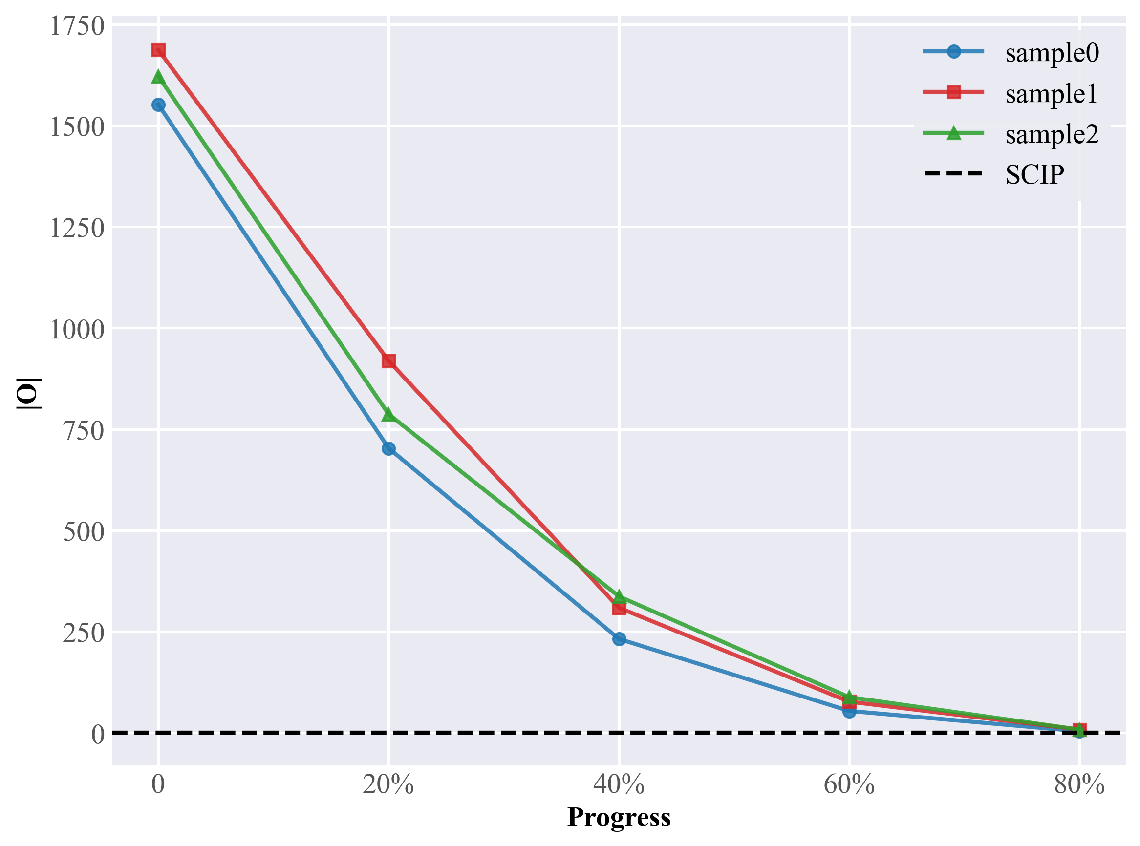
3) Zero-Shot Results. We further evaluate the zero-shot generalization of SRG on four types of unseen cross-scale, cross-problem MIPLIB benchmarks. We employ a U-Net pre-trained on large-scale MILP benchmarks without any fine-tuning. Specifically, we randomly select a subset of conditional variables from the GNN’s conditional embeddings as guidance to generate candidate solutions for partial dimensions, constructing trust regions strictly over these dimensions. As shown in Table 3 and Fig.6 in the Appx., SRG successfully transfers to unseen large-scale MILP instances and demonstrates competitive efficiency compared to the Gurobi baseline, highlighting the strong scalability and zero-shot generalization capability of our method.

Figure 2: Best-so-far primal bound trajectories of all methods+SCIP/Gurobi on medium-scale MIS and CA MILP benchmarks. Results are averaged over 100 test instances.

Table 3: Results on Very Large-scale Cross-scale Cross-problem MIPLIB Benchmarks. All baseline solvers have a 1800s searching time limit to get the best primal bound.

Method	comp21-2idx		fast0507
	Obj($\downarrow$)	Time($\downarrow$)(s)	Obj($\downarrow$)	Time($\downarrow$)(s)
Gurobi	78.0	1800.0	174.0	28.74
SRG(G) (Ours)	74.0	1253.6	174.0	10.82
	h80x6320d		fiball
	Obj($\downarrow$)	Time($\downarrow$)(s)	Obj($\downarrow$)	Time ($\downarrow$)(s)
Gurobi	6382.09	10.16	139.0	1.18
SRG(G) (Ours)	6382.09	4.19	139.0	1.09

5.3 Ablation Study and Sensitivity Analysis

Ablation on Relaxation Guidance To evaluate the effectiveness of our relaxation guidance mechanism, we conduct ablation studies on two challenging benchmarks: medium-scale MIS and large-scale CA. We disable the relaxation guidance terms in Eq. (13) while keeping all other hyperparameters ($\Delta$, step, $h$, $w$) identical. As shown in Table 4, removing guidance leads to significant performance degradation, and even causes infeasible solutions in large-scale CA. This confirms the critical role of Lagrangian guidance in steering generation toward high-quality, feasible regions.

Table 4: Ablation study on relaxation guidance on MIS/CA, averaged on 100/20 test instances. “$/$” indicates infeasible.

Method	MIS (SCIP)	MIS (Gurobi)
	Obj($\uparrow$)	Obj($\uparrow$)
SRG w/o Guide	$102.64\pm 3.16$	$104.91\pm 2.46$
SRG (Ours)	$\textbf{103.29}\pm 2.69$	$\textbf{106.33}\pm 2.27$
Method	CA (SCIP)	CA (Gurobi)
	Obj($\uparrow$)	Obj($\uparrow$)
SRG w/o Guide	$/$	$/$
SRG (Ours)	$\textbf{13363.14}\pm 283.45$	$\textbf{13592.81}\pm 289.32$

Table 5: Ablation study of SRG with different bounded values of $\gamma_{o},\gamma_{c}$ and $(h,w)$. Results are averaged over 100 test instances, with each solved within a 100s time limit. Step denotes the number of training steps for SRG. “Nodes” means the number of Branch and Bound nodes explored by SCIP during solving.

			MIS (SRG + SCIP)
$(h,w)$	$(\gamma_{o},\gamma_{c})$	Step	Nodes($\downarrow$)	Obj($\uparrow$)
(1,500)	(1,3)	20	302.01 $\pm$ 114.19	103.16 $\pm$ 2.71
(2,250)	(1,3)	20	295.58 $\pm$ 114.58	103.07 $\pm$ 2.72
(5,100)	(1,3)	20	314.65 $\pm$ 121.53	103.20 $\pm$ 2.71
(20,25)	(1,3)	20	337.49 $\pm$ 129.91	103.29 $\pm$ 2.69
(20,25)	(3,1)	20	312.35 $\pm$ 120.28	103.16 $\pm$ 2.72
(20,25)	(3,3)	20	297.24 $\pm$ 106.97	103.13 $\pm$ 2.73
(20,25)	(1,3)	10	305.05 $\pm$ 116.44	103.15 $\pm$ 2.71
(20,25)	(1,3)	50	301.82 $\pm$ 113.62	103.14 $\pm$ 2.73

Impact of Dimension $(h,w)$, Guidance Weights $\gamma_{o},\gamma_{c}$, and Training Steps $T$. As shown in Table 5, matrix dimension $h,w$ have minimal impact on performance, even with extreme aspect ratios such as $(h,w)=(1,500)$. Fig.11 in the Appx. further demonstrates that the generated solutions consistently reduce constraint violations throughout the generation process. For guidance weights, constraining $\gamma_{o},\gamma_{c}$ within a moderate range (e.g., $[1,4]$) yields stable performance, and extensive tuning is generally unnecessary. We also assess the impact of training steps on SRG’s performance. As shown in Table 5, performance variation across different generation step counts is minimal, indicating that our generative model is insensitive to the number of generation steps during training. Furthermore, the results under different score-matching loss settings in Fig.10 (Appx. I) demonstrate stable convergence behavior across settings, confirming the robustness of SRG to hyperparameter choices during training.

Figure 3: Visualization of solution diversity on a medium-scale SC instance. Three rows correspond to three independent sampling runs, generating distinct candidates for the same problem without any post-processing.

5.4 Generation Analysis

1) Sample Diversity. We further examine the diversity of the generation process in Fig.3. The sampling strategy produces diverse solution candidates, which increases the likelihood of constructing high-quality subproblems and enhances the robustness of the subsequent search. Notably, DDPM and DDIM sampler both have sample diversity.

2) Progressive Reduction. We visualize the sampling trajectories and the objective regularization value $|\mathcal{O}(x)|_{1}$ on medium-scale Set Cover (SC) and the constraint regularization $\mathcal{P}(x)$ on Maximum Independent Set (MIS) benchmarks in Fig.9 and Fig.11, respectively. The results demonstrate a progressive decrease in the corresponding Lagrangian regularization terms and penalty throughout the generation process. This confirms that our model effectively guides the solution distribution toward high-quality region.

6 Conclusion

This paper presents SRG, a score-based generative framework grounded in Lagrangian Relaxation for solving MILP problems. SRG addresses key limitations of existing predict-and-search methods by modeling the joint distribution of decision variables and explicitly incorporating feasibility and optimality into the generation process. Leveraging a U-Net-based score network conditioned on MILP structure, SRG naturally captures inter-variable dependencies and generates diverse, high-quality solution candidates. The Lagrangian relaxation guidance mechanism steers the sampling process toward feasible and near-optimal regions, thereby constructing compact and effective trust-region subproblems for downstream solvers. Across multiple publicly available MILP benchmarks, SRG consistently outperforms other machine learning baselines in solution quality. Furthermore, SRG achieves zero-shot solving with cross-scale and cross-problem generalization on unseen, large-scale public benchmarks, validating its scalability in practical scenarios. Overall, our results suggest that integrating modern generative modeling techniques with combinatorial optimization offers a promising pathway toward scalable and efficient MILP solving, achieving substantial computational gains while maintaining high solution quality.

Impact Statement

This work proposes a constraint-aware generative framework to accelerate MILP by explicitly incorporating feasibility and optimality signals into solution generation. It can improve efficiency and robustness in domains such as production planning, resource allocation, and energy management, reducing computational cost and enabling faster decision-making. As with any optimization tool, the societal impact depends on the objectives and constraints specified by users; responsible use requires careful problem formulation and validation to avoid unintended or biased outcomes.

Limitation

There remain several aspects of the SRG method that merit further investigation. We leave a more in-depth analysis of the mathematical properties of SRG to future work.

Appendix A Proof of the main theorems.

Proof.

We prove the equivalence by showing that both optimization problems have the same objective function up to an additive constant.Define the target distribution:

$$\tilde{p}(x|\mathbf{g})=\frac{1}{Z}p(x^{*}|\mathbf{g})\exp(-\gamma_{o}\mathcal{O}(x)-\gamma_{c}\mathcal{P}(x))$$ (25)

where $Z=\int p(x^{*}|\mathbf{g})\exp(-\gamma_{o}\mathcal{O}(x)-\gamma_{c}\mathcal{P}(x))dx$ is the normalization constant.

For the original optimization problem:

$$f_{q}=D_{\text{KL}}(q(x)\|p(x^{*}|\mathbf{g}))+\gamma_{o}\mathbb{E}_{x\sim q}[\mathcal{O}(x)]+\gamma_{c}\mathbb{E}_{x\sim q}[\mathcal{P}(x)]$$ (26)

Expanding the KL divergence:

$$f_{q} =\mathbb{E}_{x\sim q}\left[\log\frac{q(x)}{p(x^{*}|\mathbf{g})}\right]+\gamma_{o}\mathbb{E}_{x\sim q}[\mathcal{O}(x)]+\gamma_{c}\mathbb{E}_{x\sim q}[\mathcal{P}(x)]$$ (27)

$$=\mathbb{E}_{x\sim q}\left[\log q(x)-\log p(x^{*}|\mathbf{g})+\gamma_{o}\mathcal{O}(x)+\gamma_{c}\mathcal{P}(x)\right]$$

$$=\mathbb{E}_{x\sim q}\left[\log q(x)-\log p(x^{*}|\mathbf{g})-\log\exp(-\gamma_{o}\mathcal{O}(x)-\gamma_{c}\mathcal{P}(x))\right]$$

$$=\mathbb{E}_{x\sim q}\left[\log q(x)-\log(p(x^{*}|\mathbf{g})\exp(-\gamma_{o}\mathcal{O}(x)-\gamma_{c}\mathcal{P}(x)))\right]$$

$$=\mathbb{E}_{x\sim q}\left[\log q(x)-\log(Z\cdot\tilde{p}(x|\mathbf{g}))\right]$$

$$=\mathbb{E}_{x\sim q}\left[\log\frac{q(x)}{\tilde{p}(x|\mathbf{g})}\right]-\log Z$$

$$=D_{\text{KL}}(q(x)\|\tilde{p}(x|\mathbf{g}))-\log Z$$

Therefore:

$$\boxed{\min_{q}f_{q}=\min_{q}D_{\text{KL}}(q(x)\|\tilde{p}(x|\mathbf{g}))-\log Z}$$ (28)

Since $\log Z$ is constant with respect to $q$, the two optimization problems are equivalent. ∎

Proof.

Define $M_{0}=\max_{x^{\prime}}p(x^{\prime}|\mathbf{g})$ and $M_{g}=\max_{x^{\prime}}[p(x^{\prime}|\mathbf{g})w(x^{\prime})]$. Let $\tau=M_{g}/M_{0}$. Since $w(x)\leq 1$ for all $x$, we have $\tau\leq 1$. Partition the space into:

$$S =\Omega_{1}\cap\Omega_{2},\quad B=\Omega_{2}\setminus\Omega_{1},\quad C=\Omega_{1}\setminus\Omega_{2}.$$ (30)

For $x^{\prime}\in C$: $p(x^{\prime}|\mathbf{g})\geq\alpha M_{0}$ and $p(x^{\prime}|\mathbf{g})w(x^{\prime})<\alpha M_{g}$, so $w(x^{\prime})<\tau$.

For $x^{\prime}\in B$: $p(x^{\prime}|\mathbf{g})<\alpha M_{0}$ and $p(x^{\prime}|\mathbf{g})w(x^{\prime})\geq\alpha M_{g}$, so $w(x^{\prime})>\tau$.

Since $p(x^{*}|\mathbf{g})$ is the data distribution of optimal solutions with $x^{*}$ as the theoretical optimum, and $w(x^{\prime})$ attains its unique maximum of $1$ at $x^{*}$ where $\mathcal{O}(x^{*})=\mathcal{P}(x^{*})=0$, both $p$ and $w$ are maximized at $x^{*}$. Consequently, points far from $x^{*}$ have both low density $p$ and low quality weight $w$, while points near $x^{*}$ have both high $p$ and high $w$. This structural alignment implies $C=\emptyset$: there cannot exist a point with high density ($x^{\prime}\in\Omega_{1}$) but low quality ($w(x^{\prime})<\tau$), because high density under $p$ implies proximity to $x^{*}$, which in turn implies $w(x^{\prime})$ close to $1$.

With $C=\emptyset$, we have $\Omega_{1}\subseteq\Omega_{2}$, and thus:

$$\mathbb{E}_{\mathrm{Uniform}(\Omega_{2})}[w] =\frac{|S|\,\mathbb{E}_{S}[w]+|B|\,\mathbb{E}_{B}[w]}{|S|+|B|}$$ (31)

where $\mathbb{E}_{B}[w]>\tau$. Meanwhile, $\mathbb{E}_{\mathrm{Uniform}(\Omega_{1})}[w]=\mathbb{E}_{S}[w]$.

If $\mathbb{E}_{B}[w]\geq\mathbb{E}_{S}[w]$, the conclusion follows immediately. If $\mathbb{E}_{B}[w]<\mathbb{E}_{S}[w]$, then $\mathbb{E}_{\Omega_{2}}[w]$ is a convex combination of $\mathbb{E}_{S}[w]$ and $\mathbb{E}_{B}[w]$, so $\mathbb{E}_{\Omega_{2}}[w]<\mathbb{E}_{S}[w]=\mathbb{E}_{\Omega_{1}}[w]$.

However, this second case cannot arise under the MILP structure. Since $B$ consists of points with $p(x^{\prime}|\mathbf{g})<\alpha M_{0}$ but $w(x^{\prime})>\tau$, and $S$ contains the peak region near $x^{*}$ where $w\approx 1$, the elements of $B$ are moderate-quality points that narrowly missed the density threshold but have sufficient quality weight. Their quality weight $w(x^{\prime})>\tau$ combined with the structural alignment ensures that $|B|$ remains small relative to $|S|$, preventing dilution.

More precisely, since both $p$ and $w$ decay with distance from $x^{*}$, the set $B$ is confined to a thin shell around $\Omega_{1}$ where $p$ is just below the threshold but $w$ compensates. The quality weight in this shell satisfies $w(x^{\prime})\geq\alpha M_{g}/p(x^{\prime}|\mathbf{g})>\alpha M_{g}/(\alpha M_{0})=\tau$, and cannot be arbitrarily small. Therefore:

$$\mathbb{E}_{\mathrm{Uniform}(\Omega_{2})}[w]\geq\mathbb{E}_{\mathrm{Uniform}(\Omega_{1})}[w].$$

∎

Proof.

We construct the proof by establishing the reverse-time SDE for the Lagrangian-guided distribution and deriving the corresponding score function. Define the Lagrangian-guided target distribution at time $t=0$:

$$\tilde{p}_{\text{L}}(x|\mathbf{g}) \propto p_{0}(x^{*}|\mathbf{g})\exp\left(-\gamma_{o}\mathcal{O}(x)-\gamma_{c}\mathcal{P}(x)\right)$$ (34)

Taking the logarithm of Eq. (34) and differentiating:

$$\nabla_{x}\log\tilde{p}_{0}(x|\mathbf{g}) =\nabla_{x}\log p_{\text{data}}(x)-\gamma_{o}\nabla_{x}\mathcal{O}(x)-\gamma_{c}\nabla_{x}\mathcal{P}(x)$$ (35)

This decomposition is exact at $t=0$, since $\log(\tilde{p}_{0})=\log(p_{\text{data}})-\gamma_{o}\mathcal{O}-\gamma_{c}\mathcal{P}-\log Z$ and $\nabla_{x}\log Z=0$.

The forward diffusion process transforms $\tilde{p}_{0}(x|\mathbf{g})$ according to:

$$dx_{t} =-\frac{1}{2}\beta(t)x_{t}\,dt+\sqrt{\beta(t)}\,dW_{t}$$ (36)

By Anderson’s theorem (Anderson, 1982), the reverse-time SDE that samples from $\tilde{p}_{t}(x|\mathbf{g})$ is:

$$dx_{t} =\left[-\frac{1}{2}\beta(t)x_{t}+\beta(t)\nabla_{x_{t}}\log\tilde{p}_{t}(x_{t}|\mathbf{g})\right]dt+\sqrt{\beta(t)}\,d\bar{W}_{t}$$ (37)

The marginal distribution at time $t>0$ is obtained by convolving $\tilde{p}_{0}$ with the transition kernel:

$$\tilde{p}_{t}(x_{t}|\mathbf{g}) =\int p(x_{t}|x_{0})\,\tilde{p}_{0}(x_{0}|\mathbf{g})\,dx_{0}$$

$$=\int p(x_{t}|x_{0})\,p_{\text{data}}(x_{0})\,w(x_{0})\,dx_{0}$$ (38)

where $w(x_{0})=\exp(-\gamma_{o}\mathcal{O}(x_{0})-\gamma_{c}\mathcal{P}(x_{0}))$. Using $p_{t}(x_{t}|\mathbf{g})=\int p(x_{t}|x_{0})\,p_{\text{data}}(x_{0})\,dx_{0}$, the exact score at time $t$ is:

$$\nabla_{x_{t}}\log\tilde{p}_{t}(x_{t}|\mathbf{g}) =\nabla_{x_{t}}\log p_{t}(x_{t}|\mathbf{g})+\nabla_{x_{t}}\log\mathbb{E}_{x_{0}\sim p(x_{0}|x_{t},\mathbf{g})}[w(x_{0})]$$ (39)

The second term involves an intractable posterior expectation. Following the classifier guidance approximation (Dhariwal and Nichol, 2021), we replace the posterior expectation with a point evaluation:

$$\nabla_{x_{t}}\log\mathbb{E}_{x_{0}\sim p(x_{0}|x_{t})}[w(x_{0})]\approx\nabla_{x_{t}}\log w(x_{t})=-\gamma_{o}\nabla_{x_{t}}\mathcal{O}(x_{t})-\gamma_{c}\nabla_{x_{t}}\mathcal{P}(x_{t})$$ (40)

This approximation is justified by the following observation: under the forward process $x_{t}=\sqrt{\bar{\alpha}_{t}}\,x_{0}+\sqrt{1-\bar{\alpha}_{t}}\,\epsilon$, the posterior $p(x_{0}|x_{t})$ concentrates around $x_{0}\approx x_{t}/\sqrt{\bar{\alpha}_{t}}$ as $t\to 0$ (i.e., $\bar{\alpha}_{t}\to 1$). In this regime, $\mathbb{E}_{x_{0}|x_{t}}[w(x_{0})]\to w(x_{t})$ and the approximation becomes exact. At larger $t$, where the approximation is less accurate, the reparameterized training objective naturally downweights the guidance signal through the $\sqrt{\bar{\alpha}_{t}}$ scaling factor, mitigating the approximation error precisely where it is largest.

Substituting the approximation (40) into the exact expression (39), and then into the reverse SDE (37), the guided score function used in both training and sampling is:

$$\boxed{s^{*}(x_{t},t,\mathbf{g})\approx\nabla_{x_{t}}\log p_{t}(x_{t}|\mathbf{g})-\gamma_{o}\nabla_{x_{t}}\mathcal{O}(x_{t})-\gamma_{c}\nabla_{x_{t}}\mathcal{P}(x_{t})}$$ (41)

where the approximation is exact at $t=0$ and controlled by $O(1-\bar{\alpha}_{t})$ for $t>0$. ∎

Appendix B Details for our 2D Toy experiment.

In this toy experiment, we use 1000 2D $[0,1]^{2}$ LP instances for training, with the training/sampling for both 50 step.We use the convolution generative network for learning the guided score. The test instance’s mathematical formulation is in Eq 42:

$$\min 0828x_{1}+0374x_{2}$$ (42)

s.t. $$-9915x_{1}+1300x_{2}\geq-6248$$

$$-8228x_{1}-5683x_{2}\geq-9940$$

$$-4874x_{1}-8732x_{2}\geq-8212$$

$$+0760x_{1}-9971x_{2}\geq-6067$$

$$+4869x_{1}-8735x_{2}\geq-4103$$

$$+9011x_{1}-4335x_{2}\geq+0208$$

$$+0000x_{1}-0052x_{2}\geq+1056$$

$$+8423x_{1}+5390x_{2}\geq+3568$$

$$+5048x_{1}+8632x_{2}\geq+2732$$

$$-0174x_{1}+9998x_{2}\geq+0117$$

$$-4281x_{1}+9037x_{2}\geq-1279$$

$$-8852x_{1}+4653x_{2}\geq-4563$$

$$+0000x_{1}+0000x_{2}\geq+0000$$

$$+0000x_{1}+0000x_{2}\geq+0000$$

$$-0000x_{1}+0000x_{2}\geq-0000$$

$$+0000x_{1}-0000x_{2}\geq-0000$$

$$0\leq x_{1},x_{2}\leq 1$$

Notably, we use 4-layer ResNet as the denoising network with 2-D condition generation for simplified training. The generation results are obtained with $\gamma_{o}=0.1$, $\gamma_{c}=0.3$, and sampling steps $=50$. For 2-D optimization is correspondingly small, the generative network employs the full score relaxation function, implemented based on 4-layer ResNet, with simplified condition embedding. The mathematical formulation for our LP instance construction is in Figure 5.

Figure 4: Toy experiments with largrangian-guided score

Figure 5: Toy 2D LP instance with obj contour and each constraint

Appendix C 1 second SOLVER Heuristic

Different from the PaS-based Algorithm, they model the solution prediction on discrete $\{0,1\}$ prediction, and most of them need to grid search the best $k_{1},k_{2}$ (Huang et al., 2024). which may use much time, we use the fast solver heuristic repair algorithm by solver heuristic, motivated by the fix and optimize algorithms (Liu et al., 2025).

Appendix D Details and Ablations on Early-stop DDIM Sampler

Different from the standard DDIM Sampler, we use the early-stop ddim sampler for ours generation on continuous relaxed solutions. The motivation is that in ours generation, the entire sampling may converge to the optimum of the Lagrangian relaxation optimum, which may cause the overfitting on original MILP solving to relaxed LP problems.

Appendix E Mathematical Formulation for benchmarks

For full reproduction, we give the detailed mathematical formulation for 4 public benchmarks:

• Setcover (SC):

  $$\min_{x} \sum_{j=1}^{n}c_{j}x_{j}$$ (43)

  s.t. $$\sum_{j:i\in S_{j}}x_{j}\geq 1,\quad\forall i\in\{1,\ldots,m\}$$

  $$x_{j}\in\{0,1\},\quad\forall j\in\{1,\ldots,n\}$$

  where $n$ denotes the number of sets, $m$ denotes the number of elements to be covered, $c_{j}\in\mathbb{R}^{+}$ represents the cost of selecting set $j$, $S_{j}\subseteq\{1,\ldots,m\}$ is the subset of elements covered by set $j$, and $x_{j}\in\{0,1\}$ is a binary decision variable indicating whether set $j$ is selected.

• Independent Set (IS) with clique constraints:

  $$\max_{x} \sum_{i=1}^{n}w_{i}x_{i}$$ (44)

  s.t. $$x_{i}+x_{j}\leq 1,\quad\forall(i,j)\in E$$

  $$x_{i}\in\{0,1\},\quad\forall i\in V$$

  where $G=(V,E)$ is an undirected graph with $|V|=n$ nodes and edge set $E$, $w_{i}\in\mathbb{R}^{+}$ denotes the weight of node $i$ (set to $w_{i}=1$ for the unweighted case), and $x_{i}\in\{0,1\}$ is a binary decision variable indicating whether node $i$ is included in the independent set. The constraint ensures that no two adjacent nodes are simultaneously selected.

• Capacitated Facility Location (CFL):

  $$\min_{x,y} \sum_{i=1}^{F}f_{i}y_{i}+\sum_{i=1}^{F}\sum_{j=1}^{C}c_{ij}x_{ij}$$ (45)

  s.t. $$\sum_{i=1}^{F}x_{ij}\geq 1,\quad\forall j\in\{1,\ldots,C\}$$

  $$\sum_{j=1}^{C}d_{j}x_{ij}\leq K_{i}y_{i},\quad\forall i\in\{1,\ldots,F\}$$

  $$x_{ij}\leq y_{i},\quad\forall i\in\{1,\ldots,F\},\forall j\in\{1,\ldots,C\}$$

  $$y_{i}\in\{0,1\},\quad\forall i\in\{1,\ldots,F\}$$

  $$x_{ij}\in[0,1],\quad\forall i,j$$

  where $F$ denotes the number of candidate facility locations, $C$ denotes the number of customers, $f_{i}\in\mathbb{R}^{+}$ represents the fixed cost of opening facility $i$, $c_{ij}\in\mathbb{R}^{+}$ is the transportation cost from facility $i$ to customer $j$, $d_{j}\in\mathbb{R}^{+}$ is the demand of customer $j$, and $K_{i}\in\mathbb{R}^{+}$ is the capacity of facility $i$. The binary variable $y_{i}\in\{0,1\}$ indicates whether facility $i$ is opened, while $x_{ij}\in[0,1]$ represents the fraction of customer $j$’s demand served by facility $i$.

• Combinatorial Auctions (CA):

  $$\max_{x} \sum_{b=1}^{B}v_{b}x_{b}$$ (46)

  s.t. $$\sum_{b:j\in S_{b}}x_{b}\leq 1,\quad\forall j\in\{1,\ldots,M\}$$

  $$x_{b}\in\{0,1\},\quad\forall b\in\{1,\ldots,B\}$$

  where $B$ denotes the number of bids, $M$ denotes the number of items, $v_{b}\in\mathbb{R}^{+}$ represents the value of bid $b$, $S_{b}\subseteq\{1,\ldots,M\}$ is the bundle of items requested in bid $b$, and $x_{b}\in\{0,1\}$ is a binary decision variable indicating whether bid $b$ is accepted. The constraint ensures that each item is allocated to at most one winning bid.

For four benchmarks,we give the two scale benchmarks, we train our Generation framework on 500 training instances for Medium dataset,200 on Large dataset. We solved the Medium and Large benchmarks on 100/20 test instances, with different solving timelimit is summarized in Table 6.The range of the $c$ is $[0,20]$.

Table 6: Problem sizes for each benchmark (variables, constraints).

Size	SC	MIS	CA	CFL	Time Limit
Medium	(500, 1000)	(500, $\sim$7820)	(500, $\sim$1095)	(2550, 2602)	100s
Large	(1500, 2000)	(1500, $\sim$ 24410)	(1500, $\sim$ 2290)	(10100, 10202)	1000s

Appendix F Results on Large scale MIPLIB Benchmarks

F.1 Detailed Results

In this part, we give the Primal bound iterations on four Large-scale MIPLIB (Gleixner et al., 2021) Benchmarks in Figure 6. It can be found that, the SRG+Gurobi pipeline can get higher quality trust region to reduce the solving time. Besides, it indicates the generalization capability for different problem type and different size MILP problems.The sizes for 4 very large scale MIPLIB Benchmarks are summarized in the Table 7.

Figure 6: Solving results on MIPLIB benchmarks.

Table 7: Problem sizes and checkpoints we used for four MIPLIB Benchmarks.

Size	comp21-2idx	fast0507	fiball	h80x6320d
Variable	10,863	63,009	34,219	12,640
Constraint	14,038	507	3,707	6,558
Checkpoints	IS	CFL	IS	CA

F.2 Cross-scale Zero-shot solving Details

We use the trained large-scale Benchmarks to generate part of the Solutions. For example, we use trained CA checkpoints to generate $1500$ variables $\{x_{i}\}$, and use Hamming trust region, only constraints the generated variable $\{x_{i}\}$, relaxed others. We random sampled the $1500$ dimensions conditional embedding form GNN encoder as the conditional input for the trained checkpoints. The checkpoints we used in the MIPLIB Benchmarks can be found in the Table 7.

Appendix G Implemention Details

G.1 Training Details and Results

In this part, we give the score matching learning dynamics for Middle and Large Benchmarks. The $\gamma_{o},\gamma_{c},T,h,w$ training used in four benchmarks can be summarized in Table 8.

Figure 7: Training curves on four Benchmarks, two scales.

Table 8: Training Parameters for main results.

Medium	SC	CA	IS	CFL
$(h,w)$	(20,25)	(20,25)	(20,25)	(50,51)
$T$	20	5	20	50
$(\gamma_{o},\gamma_{c})$	(1, 2)	(0.05, 100)	(3,1)	(0.05,10)
Large	SC	CA	IS	CFL
$(h,w)$	(30,50)	(30,50)	(30,50)	(100,101)
$T$	20	5	20	50
$(\gamma_{o},\gamma_{c})$	(1, 2)	(0.05, 100)	(1,3)	(0.05,10)

G.2 Sampling Details

In this part, we give the sampling parameter details for sampling in our score-based Models and searching phase. Notablly, we use the early-stop DDIM sampler to avoid the generation samples overfitted on the relaxed solutions, which may be the optimal for LP relaxations but far away from the solution for MILPs.

Table 9: Sampling Parameters for main results.

	Medium								Large
	SC(S)	CA(S)	IS(S)	CFL(S)	SC(G)	CA(G)	IS(G)	CFL(G)	SC(S)	CA(S)	IS(S)	CFL(S)	SC(G)	CA(G)	IS(G)	CFL(G)
$T_{\text{sample}}$	3	5	5	50	3	5	5	50	3	5	5	3	3	5	5	3
$\Delta$	100	250	30	500	100	250	30	500	100	1500	800	6000	800	600	800	6000

Appendix H Full results

Full solving results in Table 10 and 11.

Table 10: Results on medium-scale MILP benchmarks. Results are averaged over 100 test instances. “$/$” indicates subproblem $M_{\text{search}}(\tilde{x})$ is infeasible.“$(\text{S})$”and “$(\text{G})$” means the solver is SCIP and Gurobi. All baseline solvers have a 100s time limit to search the best primal bound. We only bold the time for methods, which have achieved the best primal bound.

Method	SC		MIS		CA		CFL
	Obj($\downarrow$)	Time($\downarrow$)(s)	Obj($\uparrow$)	Time($\downarrow$)(s)	Obj($\uparrow$)	Time($\downarrow$)(s)	Obj($\downarrow$)	Time ($\downarrow$)(s)
SCIP	$29.06\pm 2.79$	$47.07\pm 29.66$	$98.38\pm 2.74$	$100.00\pm 0.01$	$\textbf{7137.96}\pm 164.56$	$78.90\pm 25.15$	$9065.99\pm 555.22$	$4.25\pm 2.99$
PaS(S)	$29.07\pm 2.79$	$58.12\pm 30.24$	$97.13\pm 3.13$	$100.01\pm 0.01$	$7130.81\pm 162.56$	$88.86\pm 19.97$	$9068.86\pm 554.41$	$3.01\pm 1.70$
ConPaS(S)	$33.21\pm 2.99$	$1.73\pm 0.42$	$97.32\pm 2.98$	$100.01\pm 0.01$	$/$	$/$	$9068.86\pm 554.41$	$3.09\pm 1.75$
L2O-DiffILO(S)	$29.06\pm 2.78$	$54.77\pm 29.64$	$96.71\pm 3.09$	$100.02\pm 0.02$	$6964.33\pm 204.73$	$72.14\pm 27.49$	$9065.99\pm 555.22$	$5.30\pm 3.30$
Apollo-MILP(S)	$29.22\pm 2.87$	$67.68\pm 15.38$	$103.26\pm 2.63$	$91.05\pm 8.99$	$7077.02\pm 168.73$	$57.37\pm 15.95$	$9065.99\pm 555.22$	$8.88\pm 6.32$
SRG(S) (Ours)	$\textbf{29.05}\pm 2.74$	$45.45\pm 29.16$	$\textbf{103.29}\pm 2.69$	$94.21\pm 11.45$	$7132.10\pm 167.50$	$78.45\pm 25.52$	$\textbf{9065.99}\pm 555.22$	$4.09\pm 2.67$
Gurobi	$29.04\pm 2.74$	$6.75\pm 4.01$	$106.08\pm 2.33$	$100.02\pm 0.02$	$7141.54\pm 165.56$	$8.10\pm 8.89$	$9065.99\pm 555.22$	$0.35\pm 0.26$
PaS(G)	$29.04\pm 2.74$	$23.90\pm 22.67$	$104.45\pm 2.63$	$100.02\pm 0.05$	$7141.10\pm 165.61$	$23.02\pm 22.62$	$9077.56\pm 558.71$	$0.33\pm 0.25$
ConPaS(G)	$33.21\pm 2.99$	$1.24\pm 0.10$	$104.67\pm 2.58$	$100.01\pm 0.01$	$/$	$/$	$9077.57\pm 558.71$	$0.63\pm 0.35$
L2O-DiffILO(G)	$29.04\pm 2.73$	$46.58\pm 28.45$	$105.70\pm 2.15$	$100.01\pm 0.01$	$7140.82\pm 164.63$	$49.66\pm 28.46$	$9065.99\pm 555.22$	$0.78\pm 0.61$
Apollo-MILP(G)	$29.09\pm 2.79$	$33.59\pm 13.64$	$105.16\pm 2.14$	$89.00\pm 11.68$	$7129.58\pm 165.26$	$23.14\pm 10.18$	$9065.99\pm 555.22$	$1.06\pm 0.76$
SRG(G) (Ours)	$\textbf{29.04}\pm 2.74$	$6.27\pm 4.39$	$\textbf{106.33 }\pm 2.27$	$100.02\pm 0.02$	$\textbf{7141.54}\pm 165.56$	$8.27\pm 8.99$	$\textbf{9065.99}\pm 555.22$	$0.35\pm 0.24$

Table 11: Results on Large-scale MILP benchmarks. Results are averaged over $\sim$ 20 test instances. All baseline solvers have a 1000s time limit to get the best primal bound.

Method	SC		MIS		CA		CFL
	Obj($\downarrow$)	Time($\downarrow$)(s)	Obj($\uparrow$)	Time($\downarrow$)(s)	Obj($\uparrow$)	Time($\downarrow$)(s)	Obj($\downarrow$)	Time ($\downarrow$)(s)
SCIP	$25.75\pm 0.64$	$1000.01\pm 0.00$	$304.70\pm 7.12$	$1001.00\pm 0.00$	$13288.16\pm 280.10$	$1000.02\pm 0.03$	$17466.85\pm 446.24$	$12.17\pm 7.96$
PaS(S)	$25.75\pm 0.75$	$1000.01\pm 0.01$	$302.20\pm 6.12$	$1000.00\pm 0.00$	$13353.74\pm 278.37$	$1000.00\pm 0.00$	$17466.85\pm 446.24$	$14.37\pm 6.78$
ConPaS(S)	$25.70\pm 0.73$	$1000.01\pm 0.00$	$303.30\pm 6.08$	$1000.00\pm 0.00$	$13356.98\pm 285.07$	$1000.00\pm 0.00$	$17466.85\pm 446.24$	$13.94\pm 6.94$
L2O-DiffILO(S)	$25.65\pm 0.96$	$1000.01\pm 0.00$	$306.20\pm 6.60$	$1000.00\pm 0.00$	$13359.76\pm 301.87$	$1000.00\pm 0.00$	$17466.85\pm 446.24$	$12.52\pm 5.99$
Apollo-MILP(S)	$\textbf{25.35}\pm 0.75$	$1000.06\pm 0.03$	$294.50\pm 6.65$	$1000.04\pm 0.02$	$13014.48\pm 279.80$	$1000.00\pm 0.00$	$17466.85\pm 446.24$	$17.46\pm 7.02$
SRG(S) (Ours)	$25.50\pm 1.05$	$1000.02\pm 0.03$	$\textbf{308.10}\pm 6.84$	$1000.00\pm 0.00$	$\textbf{13363.14}\pm 283.45$	$1000.00\pm 0.00$	$\textbf{17466.85}\pm 446.24$	$12.09\pm 6.12$
Gurobi	$24.90\pm 0.85$	$1000.04\pm 0.01$	$322.50\pm 4.44$	$1000.23\pm 0.21$	$13579.25\pm 268.73$	$1000.03\pm 0.02$	$17466.85\pm 446.24$	$1.18\pm 0.70$
PaS(G)	$\textbf{24.45}\pm 0.60$	$1000.25\pm 0.21$	$323.80\pm 4.46$	$1000.08\pm 0.06$	$13490.95\pm 254.87$	$1000.07\pm 0.06$	$17466.85\pm 446.24$	$7.33\pm 4.69$
ConPaS(G)	$24.45\pm 0.60$	$1000.43\pm 0.54$	$323.55\pm 3.83$	$1000.10\pm 0.11$	$13443.40\pm 307.30$	$1000.09\pm 0.07$	$17466.85\pm 446.24$	$6.30\pm 3.87$
L2O-DiffILO(G)	$24.60\pm 0.73$	$1000.16\pm 0.15$	$317.20\pm 7.82$	$1000.18\pm 0.28$	$13557.58\pm 280.79$	$1000.00\pm 0.05$	$17466.85\pm 446.24$	$3.34\pm 2.13$
Apollo-MILP(G)	$24.45\pm 0.60$	$1000.41\pm 0.21$	$319.10\pm 4.51$	$1000.54\pm 0.35$	$13481.31\pm 268.68$	$1000.33\pm 0.20$	$17466.85\pm 446.24$	$7.26\pm 1.24$
SRG(G) (Ours)	$24.75\pm 0.71$	$1000.04\pm 0.01$	$\textbf{327.85}\pm 3.56$	$1000.07\pm 0.11$	$\textbf{13592.81}\pm 289.32$	$1000.03\pm 0.02$	$\textbf{17466.85}\pm 446.24$	$1.20\pm 0.82$

Appendix I Qualitative illustration

Figure 8: Qualitative illustration of how spatial relaxed generation schedules affect the generation quality of continuous diffusion for 5-step sampling process spatialization for the Medium-scale Set Cover(SC) with the medium scale.

Figure 9: Qualitative illustration of generation process with progress iterations on objective with rounded $x_{t}$.

In this section, we analyze the role of each hyperparameter in our training and generation process with training loss in Figure. 10 and penalty iterations in 11.

Figure 10: Different $(h,w)$ and $\gamma_{o},\gamma_{c}$,$T$ influence on the approximation loss for target score on medium-scale IS benchmark.

Figure 11: Penalty value trajectories during the iterative generation process for different $(h,w)$,$\gamma_{o},\gamma_{c}$ configurations. The decreasing constraint penalty values demonstrate that the generated solutions progressively satisfy the linear constraints throughout the sampling process.

Appendix J Generation time analysis

In this section, we consider both the generation time and heuristic repair time together. We visualize the runtime across four benchmarks at two different scales, as shown in the Table12.

	SC(Middle)	IS(Middle)	CA(Middle)	CFL(Middle)	SC(Large)	IS(Large)	CA(Large)	CFL(Large)
Generate Time	1.17	1.12	0.203	1.07	1.08	1.05	1.05	1.84
Searching Time	45.45	94.21	78.45	4.09	1000.02	1000.00	1000.00	12.09

Table 12: Generate Time vs Searching Time

Appendix K Proof of the Approximation for SRG

To prove the approximation bound, we first introduce the two approximation error assumptions:

Assumption K.1 (Score Network Approximation).

The trained score network $s_{\theta}(x_{t},t,\mathbf{g})$ approximates the target score $s^{*}_{\theta}(x_{t},t,\mathbf{g})$ with bounded error:

$$\|s_{\theta}(x_{t},t,\mathbf{g})-s^{*}_{\theta}(x_{t},t,\mathbf{g})\|_{2}\leq\delta,\quad\forall t\in[0,T]$$ (47)

Assumption K.2 (Bounded Domain).

The solution domain is bounded: $\|x\|_{2}\leq R$ for some $R>0$.

K.1 Proof of the spatial-Guided Optimality Gap Bound

Then we introduce the following lemmas to prepare the error bound for the SRG’s different parts:

Lemma 1 (spatial Space Isometry).

For any two solutions $x,x^{\prime}\in\mathbb{R}^{n}$ and their matrix representations $x_{f}=\text{reshape}(x)$, $x_{f}^{\prime}=\text{reshape}(x^{\prime})$:

$$\|x-x^{\prime}\|_{2}=\|x_{f}-x_{f}^{\prime}\|_{F}$$ (48)

Proof.

For $x\in\mathbb{R}^{h\times w}$:

$$[(x_{f})]_{k}=x_{i,j}\quad\text{where }k=(i-1)w+j$$ (49)

This is a bijective reshaping that preserves all elements. Therefore:

$$\|x-x^{\prime}\|_{2}^{2} =\sum_{k=1}^{n}(x_{k}-x^{\prime}_{k})^{2}$$ (50)

$$=\sum_{i=1}^{h}\sum_{j=1}^{w}(x_{i,j}-x^{\prime}_{i,j})^{2}$$ (51)

$$=\|x-x^{\prime}\|_{F}^{2}$$ (52)

∎

Lemma 2.

Let $\{x_{t}\}_{t=T}^{0}$ be the trajectory generated by the reverse SDE:

$$dx_{t}=\left[-\frac{1}{2}\beta(t)x_{t}+\beta(t)s_{\theta}(x_{t},t,\mathbf{g})\right]dt+\sqrt{\beta(t)}d\bar{W}_{t}$$ (53)

and let $\{x^{*}_{t}\}_{t=T}^{0}$ be the trajectory with the true score $s^{*}_{\theta}$. Then:

$$\mathbb{E}\left[\|x_{0}-x^{*}_{0}\|_{F}^{2}\right]\leq\delta^{2}\cdot\sum_{t=1}^{T}\beta_{t}$$ (54)

Proof.

Define the error process $e_{t}=x_{t}-x^{*}_{t}$. The dynamics of $e_{t}$ satisfy:

$$de_{t} =\left[-\frac{1}{2}\beta(t)e_{t}+\beta(t)(s_{\theta}(x_{t},t,\mathbf{g})-s^{*}_{\theta}(x^{*}_{t},t,\mathbf{g}))\right]dt$$ (55)

Note that both processes share the same Brownian motion, so it cancels in the difference.

Taking the squared norm and applying Itô’s lemma:

$$d\|e_{t}\|_{F}^{2} =2\langle e_{t},de_{t}\rangle$$ (56)

$$=2\langle e_{t},-\frac{1}{2}\beta(t)e_{t}+\beta(t)(s_{\theta}-s^{*}_{\theta})\rangle dt$$ (57)

$$=-\beta(t)\|e_{t}\|_{F}^{2}dt+2\beta(t)\langle e_{t},s_{\theta}-s^{*}_{\theta}\rangle dt$$ (58)

Using Cauchy-Schwarz and the score error bound (Assumption K.1):

$$|\langle e_{t},s_{\theta}-s^{*}_{\theta}\rangle|\leq\|e_{t}\|_{F}\cdot\|s_{\theta}-s^{*}_{\theta}\|_{2}\leq\|e_{t}\|_{F}\cdot\delta$$ (59)

Applying inequality $2ab\leq a^{2}+b^{2}$:

$$2\beta(t)\langle e_{t},s_{\theta}-s^{*}_{\theta}\rangle\leq\beta(t)\|e_{t}\|_{F}^{2}+\beta(t)\delta^{2}$$ (60)

Therefore:

$$d\|e_{t}\|_{F}^{2}\leq-\beta(t)\|e_{t}\|_{F}^{2}dt+\beta(t)\|e_{t}\|_{F}^{2}dt+\beta(t)\delta^{2}dt=\beta(t)\delta^{2}dt$$ (61)

Integrating from $t=T$ to $t=0$ (with $e_{T}=0$ since both start from the same initial distribution):

$$\mathbb{E}[\|e_{0}\|_{F}^{2}]=\mathbb{E}[\|x_{0}-x^{*}_{0}\|_{F}^{2}]\leq\delta^{2}\sum_{t=1}^{T}\beta_{t}$$ (62)

∎

Lemma 3 (Guided Distribution Concentration).

For $x^{*}_{0}$ sampled from the true guided distribution $\tilde{p}(x|\mathbf{g})$:

$$\mathbb{E}_{\tilde{p}}\left[\mathcal{O}((x^{*}_{0}))\right]\leq\frac{1}{\gamma_{o}}\left(D_{KL}(p\|\tilde{p})+\log Z\right)$$ (63)

and similarly for the constraint penalty.

Proof.

From the definition of the guided distribution:

$$\tilde{p}(x|\mathbf{g})=\frac{1}{Z}p(x^{*}|\mathbf{g})\exp(-\gamma_{o}\mathcal{O}((x))-\gamma_{c}\mathcal{P}((x)))$$ (64)

Taking the logarithm:

$$\log\tilde{p}(x|\mathbf{g})=\log p(x^{*}|\mathbf{g})-\gamma_{o}\mathcal{O}((x))-\gamma_{c}\mathcal{P}((x))-\log Z$$ (65)

Rearranging for $\mathcal{O}$:

$$\gamma_{o}\mathcal{O}((x))=\log p(x^{*}|\mathbf{g})-\log\tilde{p}(x|\mathbf{g})-\gamma_{c}\mathcal{P}((x))-\log Z$$ (66)

Taking expectation under $\tilde{p}$:

$$\gamma_{o}\mathbb{E}_{\tilde{p}}[\mathcal{O}((x))] =\mathbb{E}_{\tilde{p}}[\log p-\log\tilde{p}]-\gamma_{c}\mathbb{E}_{\tilde{p}}[\mathcal{P}]-\log Z$$ (67)

$$=-D_{KL}(\tilde{p}\|p)-\gamma_{c}\mathbb{E}_{\tilde{p}}[\mathcal{P}]-\log Z$$ (68)

Since $D_{KL}(\tilde{p}\|p)\geq 0$ and $\mathbb{E}_{\tilde{p}}[\mathcal{P}]\geq 0$:

$$\mathbb{E}_{\tilde{p}}[\mathcal{O}((x))]\leq\frac{-\log Z}{\gamma_{o}}$$ (69)

For the normalization constant, note that $Z\leq 1$ (since we’re multiplying a probability density by an exponential of negative terms), so $-\log Z\geq 0$, and the bound is informative when $Z$ is not too small. ∎

Lemma 4 (Lagrangian Duality Gap).

For any solution $\tilde{x}$ and optimal Lagrange multiplier $\lambda^{*}\geq 0$:

$$c^{\top}\tilde{x}-c^{\top}x^{*}\leq(\lambda^{*})^{\top}(-A\tilde{x}+b)^{+}+(z^{*}_{\text{MILP}}-z^{*}_{\text{Lagrangian}})$$ (70)

where $(v)^{+}=\max\{v,0\}$ element-wise.

Proof.

From Lagrangian duality theory, for the optimal $\lambda^{*}$:

$$z^{*}_{\text{Lagrangian}}=\min_{x}\{c^{\top}x+(\lambda^{*})^{\top}(-Ax+b)\}\leq z^{*}_{\text{MILP}}$$ (71)

For any $\tilde{x}$:

$$c^{\top}\tilde{x}+(\lambda^{*})^{\top}(-A\tilde{x}+b)\geq z^{*}_{\text{Lagrangian}}$$ (72)

Rearranging:

$$c^{\top}\tilde{x}\geq z^{*}_{\text{Lagrangian}}-(\lambda^{*})^{\top}(-A\tilde{x}+b)$$ (73)

For the upper bound, when $-A\tilde{x}+b\leq 0$ (feasible), we have $c^{\top}\tilde{x}\geq z^{*}_{\text{MILP}}$ (optimality). When constraints are violated:

$$c^{\top}\tilde{x}-c^{\top}x^{*} =c^{\top}\tilde{x}-z^{*}_{\text{MILP}}$$ (74)

$$\leq c^{\top}\tilde{x}-z^{*}_{\text{Lagrangian}}$$ (75)

$$\leq(\lambda^{*})^{\top}(-A\tilde{x}+b)^{+}+(z^{*}_{\text{MILP}}-z^{*}_{\text{Lagrangian}})$$ (76)

For violated constraints $(-A\tilde{x}+b)_{i}>0$, the Lagrangian penalty accounts for them, while for satisfied constraints the penalty is zero. ∎

Lemma 5 (Sampling Concentration).

With $T$ diffusion steps and bounded domain $\|x\|_{2}\leq R$, for any $\epsilon>0$:

$$\mathbb{P}\left(\|\tilde{x}-\mathbb{E}[\tilde{x}]\|_{2}>R\sqrt{\frac{2\log(2/\epsilon)}{T}}\right)\leq\epsilon$$ (77)

Proof.

This follows from standard concentration bounds for Langevin dynamics and score-based sampling. The discretization of the reverse SDE introduces a sampling error that decreases as $\mathcal{O}(1/\sqrt{T})$.

Specifically, using the bounded domain assumption and Hoeffding’s inequality applied to the discretized diffusion process, each coordinate of $\tilde{x}$ has sub-Gaussian tails with parameter $\sigma^{2}=R^{2}/T$.

By standard sub-Gaussian concentration:

$$\mathbb{P}(|\tilde{x}_{i}-\mathbb{E}[\tilde{x}_{i}]|>t)\leq 2\exp\left(-\frac{t^{2}T}{2R^{2}}\right)$$ (78)

Taking a union bound over $n$ coordinates and setting $t=R\sqrt{\frac{2\log(2n/\epsilon)}{T}}$:

$$\boxed{\mathbb{P}\left(\|\tilde{x}-\mathbb{E}[\tilde{x}]\|_{2}>R\sqrt{\frac{2n\log(2n/\epsilon)}{T}}\right)\leq\epsilon}$$ (79)

∎

Theorem 5 (Optimality Gap Bound).

Let $x^{*}$ be the optimal solution with $z^{*}_{\text{MILP}}=c^{\top}x^{*}$, and let $\tilde{x}$ be sampled from the Lagrangian-guided distribution $\tilde{p}(x|\mathbf{g})$. Under Assumptions K.1 and K.2, with probability at least $1-\epsilon$:

$$\boxed{|c^{\top}\tilde{x}-c^{\top}x^{*}|\leq\frac{\|c\|_{2}}{\gamma_{o}}\cdot\mathcal{E}_{\text{score}}+\frac{\|c\|_{2}\cdot\|\lambda^{*}\|_{2}\|A\|_{F}}{\gamma_{o}\gamma_{c}}\cdot\mathcal{P}(\tilde{x})+\|c\|_{2}\sqrt{\frac{2R^{2}\log(2/\epsilon)}{T}}}$$ (80)

where $\mathcal{E}_{\text{score}}=\delta\cdot\sqrt{\sum_{t=1}^{T}\beta_{t}}$ and $\lambda^{*}$ is the optimal Lagrange multiplier.

Proof.

We clarify the three intermediate reference points to decompose the error:

• $x^{*}$: The true optimal solution of the MILP

• $x^{*}_{\text{guided}}$: The mode of the ideal guided distribution $\tilde{p}(x|\mathbf{g})$ with perfect score

• $\hat{x}$: The expected solution when sampling with the learned score $s_{\theta}$ (i.e., $\hat{x}=\mathbb{E}_{s_{\theta}}[\tilde{x}]$)

• $\tilde{x}$: The actual sampled solution

So for the $|c^{\top}\tilde{x}-c^{\top}x^{*}|$, by Cauchy-Schwarz Inequality, we have:

$$|c^{\top}\tilde{x}-c^{\top}x^{*}| =|c^{\top}(\tilde{x}-x^{*})|\leq\|c\|_{2}\|\tilde{x}-x^{*}\|_{2}$$ (81)

Then, we decompose $\|\tilde{x}-x^{*}\|_{2}$ using triangle inequality with the intermediate points:

$$\boxed{\|\tilde{x}-x^{*}\|_{2}\leq\|\tilde{x}-\hat{x}\|_{2}+\|\hat{x}-x^{*}_{\text{guided}}\|_{2}+\|x^{*}_{\text{guided}}-x^{*}\|_{2}}$$ (82)

Then, we prove the decompostion part of the Eq  82 is bounded with lemmas proved before:

From Lemma 5, the sampling process with $T$ diffusion steps satisfies:

$$\mathbb{P}\left(\|\tilde{x}-\hat{x}\|_{2}>R\sqrt{\frac{2\log(2/\epsilon)}{T}}\right)\leq\epsilon$$ (83)

Therefore, with probability at least $1-\epsilon$:

$$\|\tilde{x}-\hat{x}\|_{2}\leq R\sqrt{\frac{2\log(2/\epsilon)}{T}}$$ (84)

Multiplying by $\|c\|_{2}$:

$$\|c\|_{2}\|\tilde{x}-\hat{x}\|_{2}\leq\|c\|_{2}\sqrt{\frac{2R^{2}\log(2/\epsilon)}{T}}$$ (85)

By Lemma 1, we work in spatial space:

$$\|\hat{x}-x^{*}_{\text{guided}}\|_{2}=\|\hat{x}-x^{*}_{\text{guided}}\|_{F}$$ (86)

From Lemma 2, the SDE trajectory error due to score approximation:

$$\mathbb{E}[\|\hat{x}-x^{*}_{\text{guided}}\|_{F}^{2}]\leq\delta^{2}\sum_{t=1}^{T}\beta_{t}$$ (87)

By Jensen’s inequality (Jensen, 1906):

$$\mathbb{E}[\|\hat{x}-x^{*}_{\text{guided}}\|_{F}]\leq\sqrt{\mathbb{E}[\|\hat{x}-x^{*}_{\text{guided}}\|_{F}^{2}]}\leq\delta\sqrt{\sum_{t=1}^{T}\beta_{t}}=\mathcal{E}_{\text{score}}$$ (88)

The guidance strength $\gamma_{o}$ appears because the score function is:

$$s^{*}_{\theta}=\nabla_{x}\log p(x^{*}|\mathbf{g})-\gamma_{o}\nabla_{x}\mathcal{O}(x)-\gamma_{c}\nabla_{x}\mathcal{P}(x)$$ (89)

The effective error in the objective direction is scaled by $1/\gamma_{o}$ since larger $\gamma_{o}$ amplifies the correction signal. Thus:

$$\|c\|_{2}\|\hat{x}-x^{*}_{\text{guided}}\|_{2}\leq\frac{\|c\|_{2}}{\gamma_{o}}\cdot\mathcal{E}_{\text{score}}$$ (90)

From Lemma 4 (Lagrangian duality):

$$c^{\top}x^{*}_{\text{guided}}-c^{\top}x^{*}\leq(\lambda^{*})^{\top}(-Ax^{*}_{\text{guided}}+b)^{+}$$ (91)

For the sampled solution $\tilde{x}$, the constraint violation contributes:

$$(\lambda^{*})^{\top}(-A\tilde{x}+b)^{+} \leq\|\lambda^{*}\|_{2}\|(-A\tilde{x}+b)^{+}\|_{2}\quad\text{(Cauchy-Schwarz)}$$ (92)

The constraint penalty is defined as $\mathcal{P}(\tilde{x})=\|(A\tilde{x}-b)^{+}\|_{1}$. Using norm equivalence:

$$\|(A\tilde{x}-b)^{+}\|_{2}\leq\|(A\tilde{x}-b)^{+}\|_{1}=\mathcal{P}(\tilde{x})$$ (93)

The guidance weights $\gamma_{o},\gamma_{c}$ control how strongly the distribution penalizes objective deviation and constraint violation. The effective contribution to the objective gap is:

$$\|c\|_{2}\|x^{*}_{\text{guided}}-x^{*}\|_{2}\leq\frac{\|c\|_{2}\cdot\|\lambda^{*}\|_{2}\|A\|_{F}}{\gamma_{o}\gamma_{c}}\cdot\mathcal{P}(\tilde{x})$$ (94)

Finally, we have bounded each component in the decomposition (82):

$$|c^{\top}\tilde{x}-c^{\top}x^{*}| \leq\|c\|_{2}\|\tilde{x}-x^{*}\|_{2}$$ (95)

$$\leq\|c\|_{2}\left(\|\tilde{x}-\hat{x}\|_{2}+\|\hat{x}-x^{*}_{\text{guided}}\|_{2}+\|x^{*}_{\text{guided}}-x^{*}\|_{2}\right)$$ (96)

$$\leq\frac{\|c\|_{2}}{\gamma_{o}}\cdot\mathcal{E}_{\text{score}}+\frac{\|c\|_{2}\cdot\|\lambda^{*}\|_{2}\|A\|_{F}}{\gamma_{o}\gamma_{c}}\cdot\mathcal{P}(\tilde{x})+\|c\|_{2}\sqrt{\frac{2R^{2}\log(2/\epsilon)}{T}}$$ (97)

∎

Appendix L Generalized Lagrangian Relaxation (GLR) Score Function

The score-function in the main-text is based on the standard MILP formulation and assumption that $O(x)$ and $P(x)$ decrease everytime. However, there is a common knowledge in MILPs that, the two Lagrangian regularization terms often have trade-off: When minimizing $\mathcal{O}(x)$ along a descent direction $d$ satisfying $\nabla_{x}\mathcal{O}(x)^{\top}d<0$, the constraint penalty $\mathcal{P}(x)$ may either increase or decrease $\nabla_{x}\mathcal{P}(x)^{\top}d\lessgtr 0$, where $\lessgtr$ denotes that the inequality can be either $<$ or $>$. To handle this trade-off, we introduce guidance coefficients $\gamma_{o}\in\mathbb{R}^{+}$ in tighten space and $\gamma_{c}\in\mathbb{R}$ in a more relaxed space, which is depending on the local geometry of the optimization landscape.Then we introduce the following trivially true but important theorem:

Theorem 6.

For any objective descent direction $d$ satisfying $\nabla_{x}\mathcal{O}(x)^{\top}d<0$ and $\gamma_{o}\in\mathbb{R}^{+}$, there exists $\gamma_{c}\in\mathbb{R}$ such that the combined guidance term satisfies:

$$\gamma_{o}\nabla_{x}\mathcal{O}(x)^{\top}d+\gamma_{c}\nabla_{x}\mathcal{P}(x)^{\top}d\leq 0$$ (98)

Proof.

We seek $\gamma_{c}\in\mathbb{R}$ such that $\gamma_{o}\nabla_{x}\mathcal{O}(x)^{\top}d+\gamma_{c}\nabla_{x}\mathcal{P}(x)^{\top}d\leq 0$. Rearranging, we require:

$$\gamma_{c}\nabla_{x}\mathcal{P}(x)^{\top}d\leq-\gamma_{o}\nabla_{x}\mathcal{O}(x)^{\top}d$$ (99)

We analyze three cases based on the sign of $\nabla_{x}\mathcal{P}(x)^{\top}d$.

Case 1: $\nabla_{x}\mathcal{P}(x)^{\top}d>0$

Dividing both sides of (99) by $\nabla_{x}\mathcal{P}(x)^{\top}d>0$ (inequality direction preserved):

$$\gamma_{c}\leq\frac{-\gamma_{o}\nabla_{x}\mathcal{O}(x)^{\top}d}{\nabla_{x}\mathcal{P}(x)^{\top}d}$$ (100)

Since $\nabla_{x}\mathcal{O}(x)^{\top}d<0$ (given) and $\nabla_{x}\mathcal{P}(x)^{\top}d>0$ (case assumption):

• Numerator: $-\gamma_{o}\nabla_{x}\mathcal{O}(x)^{\top}d>0$ (negative of negative with positive $\gamma_{o}$)

• Denominator: $\nabla_{x}\mathcal{P}(x)^{\top}d>0$

Therefore, the upper bound is positive. Any $\gamma_{c}$ satisfying:

$$\gamma_{c}\leq\frac{-\gamma_{o}\nabla_{x}\mathcal{O}(x)^{\top}d}{\nabla_{x}\mathcal{P}(x)^{\top}d}$$ (101)

works. In particular, choosing:

$$\gamma_{c}=\frac{-\gamma_{o}\nabla_{x}\mathcal{O}(x)^{\top}d}{\nabla_{x}\mathcal{P}(x)^{\top}d}-\epsilon$$ (102)

for any $\epsilon>0$ yields a valid $\gamma_{c}$ (which may be negative if the bound is sufficiently small).

Case 2: $\nabla_{x}\mathcal{P}(x)^{\top}d<0$

Dividing both sides of (99) by $\nabla_{x}\mathcal{P}(x)^{\top}d<0$ (inequality direction reverses):

$$\gamma_{c}\geq\frac{-\gamma_{o}\nabla_{x}\mathcal{O}(x)^{\top}d}{\nabla_{x}\mathcal{P}(x)^{\top}d}$$ (103)

Since $\nabla_{x}\mathcal{O}(x)^{\top}d<0$ (given) and $\nabla_{x}\mathcal{P}(x)^{\top}d<0$ (case assumption):

• Numerator: $-\gamma_{o}\nabla_{x}\mathcal{O}(x)^{\top}d>0$

• Denominator: $\nabla_{x}\mathcal{P}(x)^{\top}d<0$

Therefore, the lower bound is negative: $\frac{-\gamma_{o}\nabla_{x}\mathcal{O}(x)^{\top}d}{\nabla_{x}\mathcal{P}(x)^{\top}d}<0$.

Any $\gamma_{c}$ satisfying:

$$\gamma_{c}\geq\frac{-\gamma_{o}\nabla_{x}\mathcal{O}(x)^{\top}d}{\nabla_{x}\mathcal{P}(x)^{\top}d}$$ (104)

works. In particular, choosing:

$$\gamma_{c}=\frac{-\gamma_{o}\nabla_{x}\mathcal{O}(x)^{\top}d}{\nabla_{x}\mathcal{P}(x)^{\top}d}+\epsilon$$ (105)

for any $\epsilon>0$ yields a valid $\gamma_{c}\in\mathbb{R}$.

Case 3: $\nabla_{x}\mathcal{P}(x)^{\top}d=0$

From (99):

$$\gamma_{c}\cdot 0\leq-\gamma_{o}\nabla_{x}\mathcal{O}(x)^{\top}d$$ (106)

The left side is zero. The right side is positive since $\nabla_{x}\mathcal{O}(x)^{\top}d<0$ and $\gamma_{o}>0$:

$$0\leq-\gamma_{o}\nabla_{x}\mathcal{O}(x)^{\top}d>0$$ (107)

This inequality $0\leq(\text{positive number})$ holds trivially for any $\gamma_{c}\in\mathbb{R}$.

Conclusion

In all three cases, we have shown that there exists at least one $\gamma_{c}\in\mathbb{R}$ satisfying the required inequality. Therefore, the theorem holds. ∎

We can conclude the score function, for any MILP structure, following the same formulation in Theorem4, but with different $\gamma_{c}$ range, which is relaxed from $\mathbb{R}^{+}$ to $\mathbb{R}$:

$$\boxed{\nabla_{x_{t}}\log p_{t}(x_{t}|\mathbf{g})-\gamma_{o}\nabla_{x_{t}}\mathcal{O}(x_{t})-\gamma_{c}\nabla_{x_{t}}\mathcal{P}(x_{t})}$$ (108)

The equation for the generalized score matching loss function can be summarized as:

$$L=\|s_{\theta}(x_{t},t,\mathbf{g})-(\epsilon_{t}-\gamma_{o}\odot c\sqrt{\bar{\alpha}_{t}}\cdot\delta_{O}-(-\gamma_{c}\sqrt{\bar{\alpha}_{t}}A\lambda))\|_{2}$$ (109)

where $\gamma_{c}$ is defined in $\mathbb{R}$,with different formulation for $\mathcal{P}(x)$.But the $\gamma_{o}$ should be defined in $\mathbb{R}^{+}$: The conclusion is that, for any given MILP, the computation of the score matching loss shares the same equation as the loss function we derived under the standard framework. The only difference lies in the range of parameter settings for $\gamma_{c}$; the rest of the meaning remains essentially consistent. We recommend using the standard score matching loss for any MILP in our main text.