VideoDetective: Clue Hunting via both Extrinsic Query and Intrinsic Relevance for Long Video Understanding

Abstract

Long video understanding remains challenging for multimodal large language models (MLLMs) due to limited context windows, which necessitate identifying sparse query-relevant video segments. However, existing methods predominantly localize clues based solely on the query, overlooking the video’s intrinsic structure and varying relevance across segments. To address this, we propose VideoDetective, a framework that integrates query-to-segment relevance and inter-segment affinity for effective clue hunting in long-video question answering. Specifically, we divide a video into various segments and represent them as a visual–temporal affinity graph built from visual similarity and temporal proximity. We then perform a Hypothesis–Verification–Refinement loop to estimate relevance scores of observed segments to the query and propagate them to unseen segments, yielding a global relevance distribution that guides the localization of the most critical segments for final answering with sparse observation. Experiments show our method consistently achieves substantial gains across a wide range of mainstream MLLMs on representative benchmarks, with accuracy improvements of up to 7.5% on VideoMME-long. Our code is available at https://videodetective.github.io/.

¹Nanjing University
²Institute of Automation, Chinese Academy of Sciences
yangruoliu1@gmail.com, bradyfu24@gmail.com
https://videodetective.github.io/

Figure 1: Overview of VideoDetective. Given a query, we (1) divide the video into segments and construct a spatio-temporal affinity graph from visual similarity and temporal proximity; (2) iteratively observe video segments and propagate the relevance scores over the graph to update a global belief field, guiding next observation via a hypothesis–verification–refinement loop to recover missing clues; and (3) aggregate a compact multimodal evidence set (query-relevant frames + related text) for MLLM to produce a clue-grounded answer.

1 Introduction

Long video understanding has become a central topic in the multimodal community, and a growing number of MLLMs tailored for long-video understanding (Chen et al., 2024a; Zhang et al., 2024a; Shen et al., 2025; Shu et al., 2025) have emerged. Despite this progress, processing massive information within limited context windows remains a critical challenge. As a result, many query-driven approaches focus on locating only the query-relevant clue segments, thereby substantially reducing the effective context length. However, reliably localizing such clues without exhaustively understanding the entire video is inherently difficult, especially for questions requiring complex reasoning.

Most existing methods (Wang et al., 2025a; Liu et al., 2025) a unidirectional query-to-video search paradigm, matching frames or segments as clues purely based on query information. For example, keyframe selection methods (Awasthi et al., 2022; Tang et al., 2025) aim to sample frames with more significant visual information; retrieval-based methods (Luo et al., 2024; Jeong et al., 2025) convert multimodal video content into text and retrieve clues via textual similarity; and agent approaches (Fan et al., 2024; Wang et al., 2024, 2025d; Yuan et al., 2025; Zhi et al., 2025) leverage LLM-based reasoning and external tools to iteratively collect and interpret clues. However, these paradigms share a common limitation: they largely emphasize query-to-content matching while overlooking the video’s intrinsic structures. A video is not merely a linear sequence of isolated frames; it exhibits coherent temporal dynamics and causal continuity. Such internal structure can be exploited to “see the whole from a part,” enabling models to maintain global understanding from sparse observations.

Motivated by this insight, we avoid assuming that a single, prior-driven step can directly pinpoint the truly informative regions, or that the process must restart from scratch once an early guess proves incorrect. Instead, we jointly leverage the query and the video’s intrinsic inter-segment correlations, using sparse observations to model the query-relevance distribution over the entire video. In this way, each observed segment contributes information gain as much as possible under a limited observation budget.

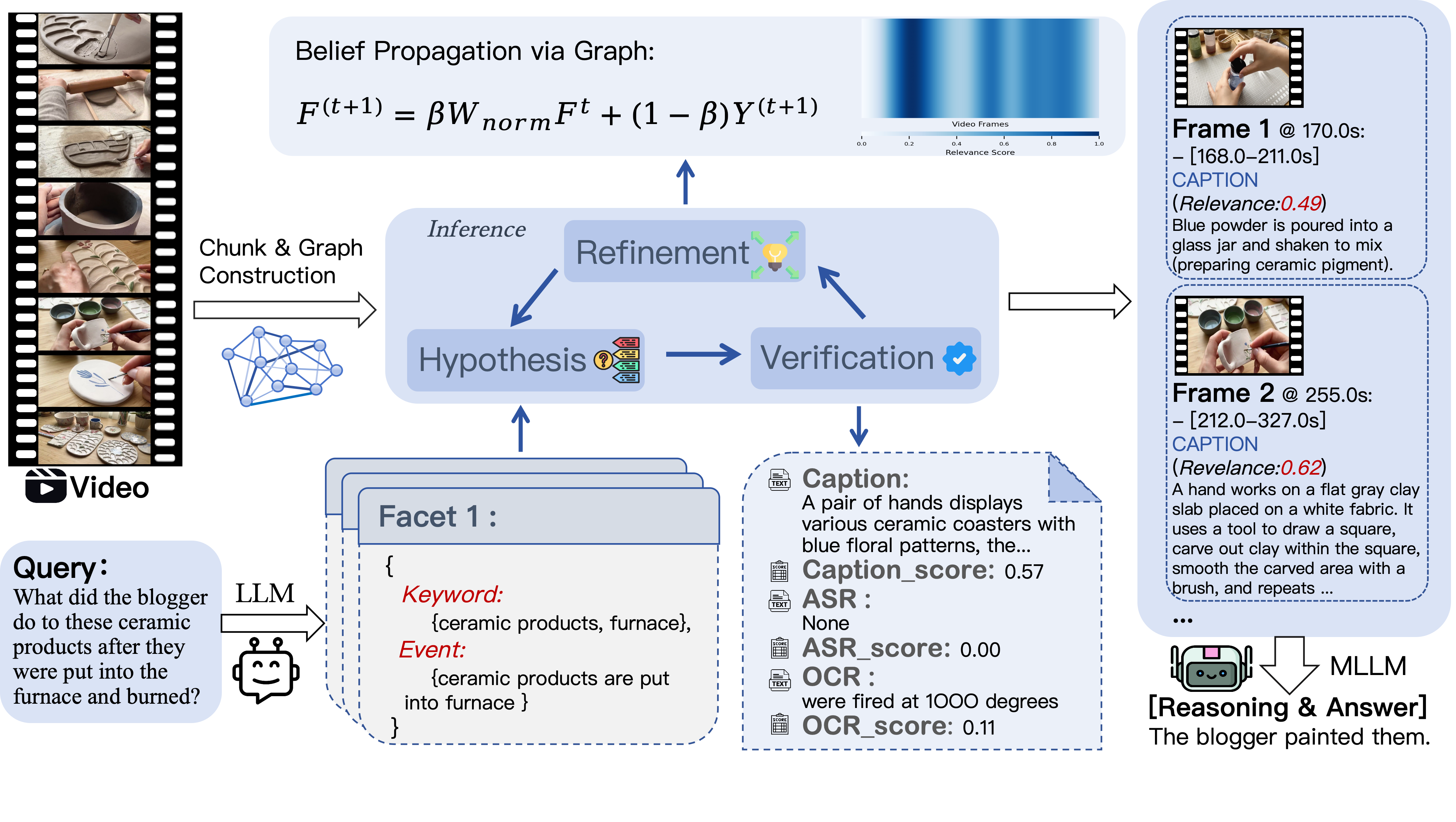
We propose VideoDetective, an inference framework that integrates both extrinsic query relevance and intrinsic video correlations to more accurately localize true clue segments, achieving “See Less but Know More”. Specifically, VideoDetective models the video as a Spatio-Temporal Affinity Graph, explicitly encoding both visual semantics and temporal continuity. Guided by this graph, the framework executes an iterative “Hypothesis-Verification-Refinement” loop: (1) Hypothesis: initially choose anchor segments based on query-guided prior similarity and iteratively select the next most informative segments as the anchor; (2) Verification: extract multi-source information (e.g., visual captions, OCR, ASR) from anchor segments to verify their local relevance and compute clue scores; (3) Refinement: propagate the relevance of visited segments to unvisited ones via graph diffusion (Zhou et al., 2004; Kipf, 2016) thereby updating the global belief field (i.e., a global relevance map over video segments). In summary:

• We propose a long-video inference framework that integrates extrinsic query with intrinsic video structure. By modeling the video as a Spatio-Temporal Affinity Graph, we exploit internal correlations to guide effective clues localization according to the query.

• We introduce graph diffusion within a “Hypothesis-Verification-Refinement” loop. This mechanism propagates sparse relevance scores from anchor segments across the graph to dynamically update the global belief field, allowing the model to progressively recover global semantic information from sparse observations.

• We demonstrate that VideoDetective is a plug-and-play framework that consistently improves performance across diverse MLLM backbones. Experiments on representative long-video benchmarks show that our method delivers substantial gains for various baseline models, achieving accuracy improvements of up to 7.5% on VideoMME-long.

2 Related Work

Multimodal Large Language Models. MLLMs (Hurst et al., 2024; Lin et al., 2024; Bai et al., 2025b; Comanici et al., 2025) combine visual encoders (Radford et al., 2021; Zhai et al., 2023)with LLMs(Achiam et al., 2023; Liu et al., 2024a; Yang et al., 2025), achieving remarkable progress in vision-language tasks. However, most MLLMs struggle with long-form content due to attention complexity and limited context windows. While some recent models (Chen et al., 2024a; Shen et al., 2025; Comanici et al., 2025) extend context window length to millions of tokens, the computational cost remains prohibitive for dense sampling.

Long Video Understanding. Long video understanding remains challenging due to the long temporal horizon and limited context budgets. Recent advances in training-free long video understanding methods can be roughly categorized into three main paradigms. Key-frame sampling and token compression methods (Awasthi et al., 2022; Shen et al., 2024; Tang et al., 2025; Tao et al., 2025; Wang et al., 2025c) adaptively sample frames or compress tokens to fit context windows, but at the risk of missing critical clues. Retrieval-augmented methods (Luo et al., 2024; Jeong et al., 2025) convert video’s content to text and use text-based retrieval to augment generation, but require full-video preprocessing and are limited by information gap from multi-modality to single modality. Recent agent-based methods (Fan et al., 2024; Wang et al., 2024, 2025d; Yuan et al., 2025; Zhi et al., 2025) explore multi-step reasoning based on LLM planning and tool use, but lack robustness to distractions.

3 Methodology

3.1 Overview

To efficiently combine both extrinsic query and intrinsic relevance to localize query-related video segments, we formulate long-video QA as iterative relevance state estimation on a visual–temporal affinity graph $G=(\mathcal{V},\mathcal{E})$ (Algorithm 1). Given a video $V$, we treat its segments $\{c_{i}\}_{i=1}^{K}$ as nodes $\mathcal{V}$ and fuse visual similarity with temporal continuity as edges $\mathcal{E}$. We maintain two state vectors at step $t$:

• Injection Vector $\boldsymbol{Y}^{(t)}\in\mathbb{R}^{K}$: A sparse observation vector initialized by priors. It records the verified relevance scores ($Y^{(t)}_{i}\leftarrow s_{i}$) at visited segment nodes and serves as the source signal for diffusion.

• Belief Field $\boldsymbol{F}^{(t)}\in\mathbb{R}^{K}$: A dense global relevance scores distribution inferred from $\boldsymbol{Y}^{(t)}$ by propagating information over the affinity graph. Each entry $F^{(t)}_{i}$ estimates how likely segment $c_{i}$ contains query-relevant evidence, even if $c_{i}$ has not been directly observed.

In each iteration, we verify a selected anchor segment via text matching (§3.3.2), update the injection state $\boldsymbol{Y}$, and perform graph diffusion (§3.3.3) to refine the belief field $\boldsymbol{F}$. Finally, we aggregate top-ranked segments from $\boldsymbol{F}$ for the downstream MLLM to generate the answer.

3.2 Visual-Temporal Affinity Graph Construction

To model the continuous global belief field from sparse segment observations, we construct a Visual–Temporal Affinity Graph, which is essentially the topological structure that captures the intrinsic associations between video segments. This graph defines how relevance scores should propagate from observed anchor segments to unvisited ones.

3.2.1 Video Segmenting & Node Representation

To obtain the discrete nodes for our graph, we divide the video into $K$ semantic segments $\{c_{i}\}_{i=1}^{K}$ based on visual similarity. Specifically, we extract $T$ frames $\{x_{t}\}_{t=1}^{T}$ and leverage the SigLIP encoder (Zhai et al., 2023) to generate frame features $f_{t}\in\mathbb{R}^{D}$. We identify segment boundaries where the cosine similarity between adjacent frames drops below a threshold (i.e., $\langle f_{t},f_{t+1}\rangle<\theta_{\mathrm{sim}}$), and subsequently merge fragmented segments shorter than $L_{\min}$. Finally, each node $i$ is represented by $h_{i}=\operatorname{norm}\left({|c_{i}|}^{-1}\sum_{t\in c_{i}}f_{t}\right)$

3.2.2 Affinity Matrix

We construct an edge weight matrix $\mathbf{W}\in\mathbb{R}^{K\times K}$ to define inter-node relations and govern how relevance scores diffuse across the graph. The ideal graph structure should satisfy: (1) visually similar segments are highly connected to support cross-temporal information sharing; (2) temporally adjacent segments remain connected to leverage the temporal coherence of events.

 

Algorithm 1 VideoDetective: Clue Hunting via both Extrinsic Query and Intrinsic Relevance for Long Video Understanding

 

0:  Video $V$, Question $q$, Iteration steps budget $B$

0:  Answer $a$

1:  Preprocessing:

2:     Chunk $V$ into $K$ segments $\{c_{i}\}_{i=1}^{K}$ with features $\{h_{i}\}$

3:     Generate global event timeline and node descriptions $\{e_{i}\}$

4:     Build affinity graph $\mathbf{W}$; decompose $q\rightarrow\{(\mathcal{K}_{r},\mathcal{P}_{r})\}_{r=1}^{R}$

5:     Initialize injection scores $\boldsymbol{Y}^{(0)}\leftarrow\textsc{PriorScore}(q,\{e_{i}\})$; $\boldsymbol{F}^{(0)}\leftarrow\boldsymbol{Y}^{(0)}$

6:  Initialize state: $\mathcal{M}\leftarrow\{1,\dots,R\}$; $\boldsymbol{v}\leftarrow\boldsymbol{0}$ {$\mathcal{M}$: unresolved facets; $\boldsymbol{v}$: visited mask}

7:  Initialize anchors: for each facet $r$, $i^{\star}\leftarrow\arg\max_{i}(Y^{(0)}_{r})_{i}$

8:  for $t=1$ to $B$ do

9:  if $\mathcal{M}=\emptyset$ and $\sum_{j=1}^{K}v_{j}=K$ then

10:   break

11:  end if

12:  Hypothesis (select next segment):

13:  if $\mathcal{M}\neq\emptyset$ then

14:   $i^{\star}\leftarrow\arg\max_{j:\,v_{j}=0,\,\tilde{W}_{ij}>0}\;\tilde{W}_{ij}\cdot F^{(t)}_{j}$ {next anchor, Eq. (6)}

15:   Select a facet $r\in\mathcal{M}$

16:  else

17:   $\mathcal{M}\leftarrow\mathcal{M}\setminus\{r\}$ {facet verified}

18:   $i^{\star}\leftarrow\arg\max_{j}\;F^{(t-1)}_{j}\cdot(1-v_{j})$ {gap filling, Eq. (7)}

19:  end if

20:  Verification (observe and score):

21:     $(s_{i},\;need\_more)\leftarrow\textsc{Observe}(i,q,\mathcal{K}_{r},\mathcal{P}_{r})$ {extract multimodal evidence and compute score, §3.3.2}

22:  Refinement (update hypothesis state):

23:     Inject observation: $Y^{(t)}_{i}\leftarrow s_{i}$; $v_{i}\leftarrow 1$

24:     Propagate: $\boldsymbol{F}^{(t)}\leftarrow\textsc{Diffuse}(\boldsymbol{Y}^{(t)},\mathbf{W})$

25:  end for

26:  Answer: $\mathcal{S}\leftarrow\textsc{GraphNMS}(\boldsymbol{F}^{(t)})$; return $\textsc{MLLM}(\mathcal{S},q)$

 

Visual affinity: we define visual affinity as cosine similarity and truncate negative values to avoid spurious anti-correlations, using $\ell_{2}$-normalized node features $\{h_{i}\}$:

$$(\mathbf{W}^{\mathrm{sim}})_{ij}=\max\{0,\langle h_{i},h_{j}\rangle\}.$$ (1)

Temporal affinity: We model temporal proximity using an exponentially decaying kernel (Belkin & Niyogi, 2003):

$$(\mathbf{W}^{\mathrm{time}})_{ij}=\exp\!\left(-\frac{|t_{i}-t_{j}|}{\tau}\right),$$ (2)

where $t_{i}$ denotes the center time of segment $c_{i}$, and $\tau$ controls the temporal influence range.

Fusion and Sparsification: We synthesize the final affinity graph via a weighted combination $\mathbf{W}=\alpha\mathbf{W}^{\mathrm{sim}}+(1-\alpha)\mathbf{W}^{\mathrm{time}}$, where $\alpha$ balances visual semantics and temporal continuity. To ensure robust diffusion and mitigate over-smoothing (Li et al., 2018), we explicitly remove self-loops ($W_{ii}=0$), sparsify the graph by retaining only the top-$k$ connections per row, and symmetrize the result via $\tilde{\mathbf{W}}\leftarrow(\tilde{\mathbf{W}}+\tilde{\mathbf{W}}^{\top})/2$ to enforce bidirectional information flow.

Symmetric normalization: To ensure diffusion convergence, we adopt the symmetric normalized Laplacian form (Zhou et al., 2004). Let $\mathbf{D}$ be the degree matrix with $D_{ii}=\sum_{j}\tilde{W}_{ij}$, and define

$$\mathbf{W}_{\mathrm{norm}}\triangleq\mathbf{D}^{-\frac{1}{2}}\,\tilde{\mathbf{W}}\,\mathbf{D}^{-\frac{1}{2}}.$$ (3)

This normalization ensures that the spectral radius of $\mathbf{W}_{\mathrm{norm}}$ is $\leq 1$, making the iterative diffusion process converge within bounds (Chung, 1997).

3.3 Update Global Belief Field via Hypothesis-Verification-Refinement Iteration

Based on the constructed graph, we need to quantify the relevance scores distribution of the entire video with the user query. To achieve it with sparse observations, we design a Hypothesis-Verification-Refinement loop (Figure 1). In each iteration, it selects informative anchor segments (Hypothesis), observes the content to verify the presence of query keywords and measure relevance scores (Verification), and propagates these scores across the graph to update the global belief field (Refinement), progressively recovering the complete semantic structure of the video.

3.3.1 Hypothesis: Prior Injection & Dynamic Anchor Selection

The Hypothesis phase is meant for selecting anchor segments that serve as information priors for subsequent verification and refinement. To ensure precise localizing, we first decompose the user query into semantic facets. Guided by these facets, we adopt a stage-dependent selection strategy: we employ Facet-Guided Initialization to determine the initial anchor before the iterative loop ($t=0$), and transition to Informative Neighbor Exploration or Global Gap Filling during the iterations ($t>0$).

Query Decomposition. To ensure precise clues grounding, we employ an LLM to rewrite the query $q$ into $R$ distinct semantic facets $\{f_{r}\}_{r=1}^{R}$. For each facet $f_{r}$, we extract two complementary components: a keyword set $\mathcal{K}_{r}$ and a semantic description set $\mathcal{P}_{r}$ :

$$q\xrightarrow{\text{LLM}}\{f_{r}\}_{r=1}^{R},\quad\text{where }f_{r}=(\mathcal{K}_{r},\mathcal{P}_{r}).$$ (4)

By isolating these components, we can verify clues for specific entities or events separately, preventing information interference between different segments.

Selection Policy I: Facet-Guided Initialization. To localize initial anchor segment, we compute a hybrid prior score for each facet $r$ by fusing sparse visual matching (keywords to frames) and dense semantic matching (descriptions to timeline) (Arivazhagan et al., 2023):

$$(Y^{\mathrm{prior}}_{r})_{i}=\alpha\cdot\max_{w\in\mathcal{K}_{r}}\langle\phi_{T}(w),h_{i}\rangle+(1-\alpha)\cdot\max_{p\in\mathcal{P}_{r}}\langle\psi(p),\psi(e_{i})\rangle,$$ (5)

where $\phi_{T}$ is the SigLIP text encoder, $\psi$ is the semantic encoder, and $e_{i}$ are descriptions generated by a coarse VLM scan. We then select the initial anchor to maximize this confidence: $i^{\star(0)}=\operatorname{argmax}_{i}(Y^{\mathrm{prior}}_{r})_{i}$.

Selection Policy II: Iterative Active Sampling. During the iterative inference process ($t\geq 1$), we dynamically determine the next anchor segment for the following iteration based on the verification feedback from the previous step. We maintain a tracking set $\mathcal{M}$ for unresolved facets.

Case A: Informative Neighbor Exploration. If the VLM feedback indicates insufficient evidence (e.g., “missing keywords”) for the current facet $r\in\mathcal{M}$ in “Verification” stage, we infer that the target event likely resides in the temporal or semantic vicinity of the current anchor. We thus select the next anchor $i^{\star(t)}$from the unvisited neighbors on the affinity graph, prioritizing those with strong connections to the current belief state:

$$i^{\star(t)}\leftarrow\operatorname*{arg\,max}_{j\in\mathcal{U},\,\tilde{W}_{i^{\star}j}>0}\left(\tilde{W}_{i^{\star}j}\cdot F^{(t-1)}_{j}\right),$$ (6)

where $\mathcal{U}$ denotes the set of unvisited segments.

Case B: Global Gap Filling. Conversely, if the evidence for facet $r$ is confirmed, we remove it from $\mathcal{M}$. Once all facets are successfully resolved ($\mathcal{M}=\emptyset$) while the iteration budget remains, we switch to a global exploration strategy to uncover potential blind spots. We greedily select the unvisited node $i^{\star(t)}$ with the highest global belief score:

$$i^{\star(t)}=\operatorname*{arg\,max}_{i}\left(F^{(t-1)}_{i}\cdot(1-v^{(t-1)}_{i})\right),$$ (7)

where $v^{(t-1)}_{i}\in\{0,1\}$ is a binary mask indicating whether node $i$ has been visited. This mechanism ensures that promising regions missed by facet-specific searches are eventually captured.

3.3.2 Verification: Multimodal Evidence Extraction and Relevance Scoring.

For each selected anchor node $i$, we perform verification to check whether the observed segment covers the keywords derived from the semantic facet and compute the anchor’s relevance score. We extract a multi-source evidence set $\mathcal{E}_{i}=\{e_{i}^{\mathrm{cap}},\,e_{i}^{\mathrm{ocr}},\,e_{i}^{\mathrm{asr}}\}$: (1) we employ the VLM to perform a dual-purpose task: generating a detailed scene description while simultaneously verifying alignment with the current facet, explicitly outputting “missing keywords $x$” if the keywords $x$ in $\mathcal{K}_{r}$ are not observed in the visual content; (2) we extract on-screen text via EasyOCR (JaidedAI, 2023); (3) we align pre-generated speech transcripts using Whisper (Radford et al., 2023).

Relevance Scoring. Since critical clues are distributed across visual, textual, and acoustic channels, single-modal observations are often insufficient. We extract a multi-source evidence set $E=\{e_{cap},e_{ocr},e_{asr}\}$. For each evidence item $e\in E$, we design a “source-aware” scoring mechanism to measure its relevance.

Lexical Similarity. We use an IDF-weighted lexical overlap score between evidence text and keywords to calculate lexical similarity:

$$s_{\mathrm{lex}}(e,f_{r})=\min\left(1,\frac{\sum_{t\in e\cap\mathcal{K}_{r}}\mathrm{IDF}(t)}{Z_{\mathrm{lex}}}\right),$$ (8)

where $Z_{\mathrm{lex}}$ is a normalization constant (see Appendix E.4).

Semantic Similarity. We use a text encoder $\psi(\cdot)$ (SigLIP text tower) for dense embeddings and calculate cosine similarity against semantic queries (event descriptions):

$$s_{\mathrm{sem}}(e,f_{r})=\max_{p\in\mathcal{P}_{r}}\frac{\langle\psi(e),\psi(p)\rangle}{\|\psi(e)\|_{2}\,\|\psi(p)\|_{2}+\epsilon}.$$ (9)

Source-aware Fusion. Different evidence sources have different signal-to-noise ratios. OCR text is precise but sparse (high precision, low recall) and should trust lexical matching more; visual captions are the opposite (high recall, lower precision) and should trust semantic similarity more. We adopt adaptive weights $\lambda_{src}$ to get the final similarity:

$$s(e,f_{r})=\lambda_{\mathrm{src}(e)}\,s_{\mathrm{lex}}(e,f_{r})+(1-\lambda_{\mathrm{src}(e)})\,s_{\mathrm{sem}}(e,f_{r}).$$ (10)

Node aggregation. For multi-source evidence at node $i$, we take the maximum relevance as their relevance score:

$$s_{i}=\max_{e\in E_{i},\,r\in\{1,\dots,R\}}s(e,f_{r}).$$ (11)

We then inject the score into the belief field: $\boldsymbol{Y}^{(t+1)}_{i^{\star}}\leftarrow s_{i^{\star}}$, mark the node as visited, and propagate via Refinement to update the global belief $\boldsymbol{F}^{(t+1)}$.

3.3.3 Refinement: Belief Propagation via Manifold

We treat the computed relevance score of the observed anchor segment as a injection signal and diffuse it across the affinity graph to infer the relevance scores of other segments. The resulting global belief field $\boldsymbol{F}$ is optimized to satisfy two properties: (1) Consistency with the sparse observed values in $\boldsymbol{Y}$, and (2) Smoothness with respect to the graph manifold structure. Formally, we minimize the following cost function (Zhou et al., 2004; Belkin et al., 2006):

$$\mathcal{J}(\boldsymbol{F})=\underbrace{\|\boldsymbol{F}-\boldsymbol{Y}\|_{2}^{2}}_{\text{Consistency}}+\mu\underbrace{\boldsymbol{F}^{\top}\mathbf{L}\boldsymbol{F}}_{\text{Smoothness on manifold}},$$ (12)

where $\mathbf{L}=\mathbf{I}-\mathbf{D}^{-1/2}\tilde{\mathbf{W}}\mathbf{D}^{-1/2}$ is the symmetric normalized graph Laplacian. The smoothness term penalizes confidence differences between high-affinity neighbors, enabling relevance to diffuse along visual-temporal paths.

We adopt iterative diffusion for efficiency:

$$\boldsymbol{F}^{(t+1)}=\beta\,\mathbf{W}_{\mathrm{norm}}\,\boldsymbol{F}^{(t)}+(1-\beta)\,\boldsymbol{Y}^{(t+1)},$$ (13)

where $\beta=\mu/(1+\mu)\in(0,1)$ balances smoothness and consistency. With top-$k$ sparsification, $\mathbf{W}_{\mathrm{norm}}$ has $O(Kk)$ non-zeros; using sparse observation, each iteration costs $O(Kk)$, yielding $O(TKk)$ overall (with $k\ll K$)(Yedidia et al., 2003). A detailed derivation of the complexity is deferred to Appendix.

3.4 Segment Selection via Graph-NMS

Upon the completion of the iteration, we obtain the converged global belief field, which serves as the final relevance scores distribution for sampling. To extract a diverse and representative set of key segments, we apply Graph-NMS (Bodla et al., 2017). This mechanism prioritizes high-confidence regions while enforcing diversity through neighbor suppression on the affinity graph. Crucially, we explicitly retain the maximum-belief node for each query facet to guarantee that all semantic aspects are covered before feeding the aggregated evidence to the downstream MLLM.

4 Experiments

Figure 2: Performance improvements across different backbones on VideoMME-long w/o subtitle. VideoDetective consistently enhances various vision-language models across different architectures and parameter scales, demonstrating its plug-and-play capability.

4.1 Experiments Setup

Benchmarks. To comprehensively evaluate the overall performance of VideoDetective in long-video understanding, we conduct experiments on four representative benchmarks. Specifically, we evaluate on the long-video subset without subtitles (Long subset w/o subtitles) of VideoMME (Fu et al., 2025a) and LVBench (Wang et al., 2025b) without auxiliary transcripts, and complete evaluations on the validation split (Val split) of LongVideoBench (Wu et al., 2024) and the test split (Test split) of MLVU (Zhou et al., 2025).

Baselines. We compare with baselines across three tiers: proprietary models (GPT-4o (Hurst et al., 2024), Gemini-1.5-Pro (Team et al., 2024), SeedVL-1.5 (Guo et al., 2025)), large-scale open-source models ($\geq$72B parameters: Qwen2.5-VL-72B (Bai et al., 2025b), LLaVA-Video-72B (Zhang et al., 2024b)), and lightweight open-source models ($<$30B: LongVITA-16k  (Shen et al., 2025), LongVILA (Chen et al., 2024a), InternVL-2.5 (Chen et al., 2024b), etc.(Fu et al., 2025b; Li et al., 2024; Shu et al., 2025; Zhang et al., 2024b; Bai et al., 2025b, a)). We also apply VideoDetective framework to various backbones (Figure 2) to prove its effectiveness and reproduce representative methods with the same backbones for fair comparison.

Parameters setting. We set the active inference budget to 10 iterations. In each verification step, the VLM observes a local window of 9 frames. For graph construction, we use a sparsity of top-$k=8$ and a temporal decay factor $\tau=30.0$.

Evaluation Environment. API-based models (Qwen (Bai et al., 2025b, a; Yang et al., 2025), SeedVL (Guo et al., 2025), GLM (Hong et al., 2025) series) are tested via official APIs. Other open-source MLLM backbones are evaluated on NVIDIA RTX 4090 GPU clusters.

4.2 Main Results

4.2.1 Generalization across Different Backbones

To verify the universality of our approach, we applied VideoDetective to a diverse set of MLLM (Chen et al., 2024b; Liu et al., 2024b; Shen et al., 2025; Bai et al., 2025a; Qin et al., 2025; Hong et al., 2025; Guo et al., 2025; Chen et al., 2025) backbones ranging from 8B to 32B parameters. As illustrated in Figure 2, VideoDetective consistently yields performance gains across all tested models without task-specific tuning. Notably, it brings a substantial 7.5% improvement to InternVL-2.5 (8B), 7.0% to Oryx-1.5 (7B) and robust gains on other baseline models. These results demonstrate that VideoDetective functions as a plug-and-play inference framework that improves long-video performance by jointly leveraging extrinsic query-guided priors and intrinsic manifold propagation.

4.2.2 Controlled Comparison with Representative Methods

To validate the independent effectiveness of our algorithmic framework, we conduct a fair comparison between VideoDetective and other four representative long-video understanding paradigms—LVNet (Awasthi et al., 2022), Deep Video Discovery (DVD) (Zhang et al., 2025), VideoAgent (Fan et al., 2024), and VideoRAG (Luo et al., 2024)—all of them unify multimodal and textual backbones: Qwen3VL-8B and SeedVL-1.5, sampling 32 frames for the final MLLM answer generation across all methods. The experimental results demonstrate that regardless of the strength of the base model, VideoDetective also can unleash its long-video understanding potential and consistently outperforms these representative frameworks across the same backbones.

Table 1: Effectiveness Analysis across Different Backbones. We compare VideoDetective with four representative long-video understanding frameworks using two different backbones (all with 32 frames sampling to answer) on VideoMME-long w/o subtitle. Ours achieves the best performance across both model scales.

Backbone (LLM + VLM)	Method	Accuracy (%)
Qwen3-8B + Qwen3VL-8B	LVNet	40.4
	DVD	42.6
	VideoAgent	42.0
	VideoRAG	50.3
	VideoDetective	55.6
Qwen3-30B + SeedVL-1.5	LVNet	51.7
	DVD	45.4
	VideoAgent	51.7
	VideoRAG	62.0
	VideoDetective	65.6

4.2.3 Comparison with State-of-the-Art Models

Table 2: Comparison with State-of-the-Art Models. We report the accuracy (%) on four challenging long-video benchmarks of our methods and other baseline models. And the number of frames finally fed to MLLM to generate answer is 32.

Model	Param	Frames	VideoMME	LVBench	MLVU	LongVideoBench
			(Long w/o sub)		(Test)	(Val)
Proprietary Models
GPT-4o	-	384	65.3	48.9	54.9	66.7
Gemini-1.5-Pro	-	256	67.4	33.1	53.8	64.0
SeedVL-1.5	20B(A)	32	63.1	46.1	54.9	63.8
Open-Source Models ($<$ 30B)
LongVITA-16k	14B	64	54.7	-	-	59.4
LongVILA	7B	1fps	53.0	-	-	57.1
LLaVA-OneVision	7B	-	46.7	-	47.2	56.4
LLaVA-Video	7B	512	52.9	43.1	-	58.2
VideoXL	7B	1fps	52.3	42.9	45.5	50.7
Qwen2.5-VL	7B	128	53.9	36.9	45.5	51.0
Qwen3-VL	8B	32	50.2	41.1	50.1	58.9
InternVL-2.5	8B	32	50.8	39.9	52.8	59.2
VITA-1.5	7B	16	47.1	37.1	39.4	53.6
VideoDetective (Qwen3-VL)	8B	32	55.6	43.2	56.3	60.2
Open-Source Models ($\geq$ 30B)
Qwen2.5-VL	72B	128	64.6	47.4	53.8	-
LLaVA-Video	72B	64	70.3	46.1	-	63.9
VideoDetective (SeedVL-1.5)	20B(A)	32	65.6	51.3	63.8	67.9

As shown in Table 2, VideoDetective establishes a new state-of-the-art across different parameter scales. In the lightweight setting, integrating VideoDetective with Qwen3-VL-8B yields substantial gains of 5.4% and 6.2% on VideoMME and MLVU, respectively, significantly outperforming purpose-built long-video baselines such as InternVL-2.5 and LongVILA.

Most remarkably, when equipped with SeedVL-1.5 (20B), our framework achieves 67.9% accuracy on the challenging LongVideoBench (Val). This performance not only surpasses the significantly larger LLaVA-Video-72B (63.9%) by a clear margin but also outperforms leading proprietary models such as GPT-4o (66.7%) and Gemini-1.5-Pro (64.0%). These results provide compelling evidence that strategic active inference can effectively compensate for scale limitations, enabling open-source models to rival proprietary models in complex reasoning tasks.

4.3 Ablation Studies

4.3.1 Component Analysis

Table 3: Ablation Study on VideoMME-long w/o subtitle. Contribution of each core component in VideoDetective.

Configuration	Accuracy (%)	$\Delta$
VideoDetective (Full)	55.6	-
1. Graph & Propagation
w/o Graph Propagation	51.4	-4.2
2. Active Inference
w/o Facet Decomposition & Iterative Refinement	47.8	-7.8
w/o Iterative Refinement	51.0	-4.6
3. Multimodal Evidence
w/o Textual Evidence	49.9	-5.7
w/o Optimized Sampling	50.7	-4.9
Baseline (Direct Inference)	50.2	-5.4

To verify the necessity of each core component in VideoDetective, we conduct detailed ablation experiments on the VideoMME-long benchmark (Table 3). We choose the Qwen3VL-8B-Instruct as the multimodal backbone and Qwen3-8B as LLM. For the baseline, we uniformly sample 32 frames as input to Qwen3VL-8B-Instruct.

Impact of Graph Manifold Structure. Removing the graph propagation mechanism (w/o Propagation) degrades performance by 4.2%. This confirms that isolated anchor nodes observations are insufficient, and the manifold smoothness constraint is essential for inferring the relevance of unvisited regions based on sparse signals.

Necessity of Semantic Decomposition. Retaining propagation but removing query semantic decomposition (w/o Facet Decomposition) causes accuracy to degrade to 47.8%, performing even worse than the baseline. This indicates that blind similarity propagation introduces substantial noise. Our semantic facet decomposition acts as a crucial “compass,” ensuring that relevance signals propagate along semantically valid paths rather than visual similarities alone.

Efficiency of Active Iterative Loop. The “hypothesis-verification-refinement” loop is indispensable; replacing it with a single-round observation for each facet(w/o Iterative Refinement) leads to a 4.6% drop. This validates that our evidence-driven mechanism can effectively correct biases from initial retrieval through iterative feedback.

Complementarity of Multimodal Evidence. Neither relying solely on visual frames (Visual Only, 49.9%) nor adding textual evidence (detailed caption + OCR + ASR) which keep the same format as our framework to uniform frame sampling (Both frames and texts, 50.7%) can achieve optimal performance, verifying the strong complementarity between textual evidence and visual features.

4.3.2 Modality Scaling Analysis

Table 4: Modality Scaling Analysis. Performance bottleneck investigation by independently scaling LLM and Visual Encoder.

LLM	VLM	Acc. (%)	Gain
Baseline Configuration
Qwen3-8B	Qwen3-VL-8B	55.6	-
Scaling LLM
Qwen3-30B	Qwen3-VL-8B	55.8	+0.2
Scaling VLM
Qwen3-8B	SeedVL-1.5	65.1	+9.5
Scaling Both
Qwen3-30B	SeedVL-1.5	65.6	+10.0

Finally, we investigate the contribution weights of visual perception and language reasoning to long-video understanding performance (Table 4). We adopt a strategy of independently scaling the capabilities of the LLM and VLM.

The experimental results reveal asymmetry: when we fix the VLM to Qwen3-VL-8B and only upgrade the LLM from 8B to 30B, performance almost stagnates (from 55.6% increasing only marginally to 55.8%), indicating that an 8B-level LLM already owns sufficient capability to decompose queries. In contrast, when we fix the LLM at lightweight 8B and only upgrade the VLM to the stronger SeedVL-1.5, accuracy achieves a qualitative leap (surging from 55.6% to 65.1%, $\Delta$+9.5%). This powerfully demonstrates that under the VideoDetective framework, the performance ceiling bottleneck still lies in the visual model.

4.4 Efficiency Analysis

Figure 3: Token Efficiency. Comparison of accuracy versus average token consumption. VideoDetective achieves the optimal position on the efficiency-accuracy Pareto frontier.

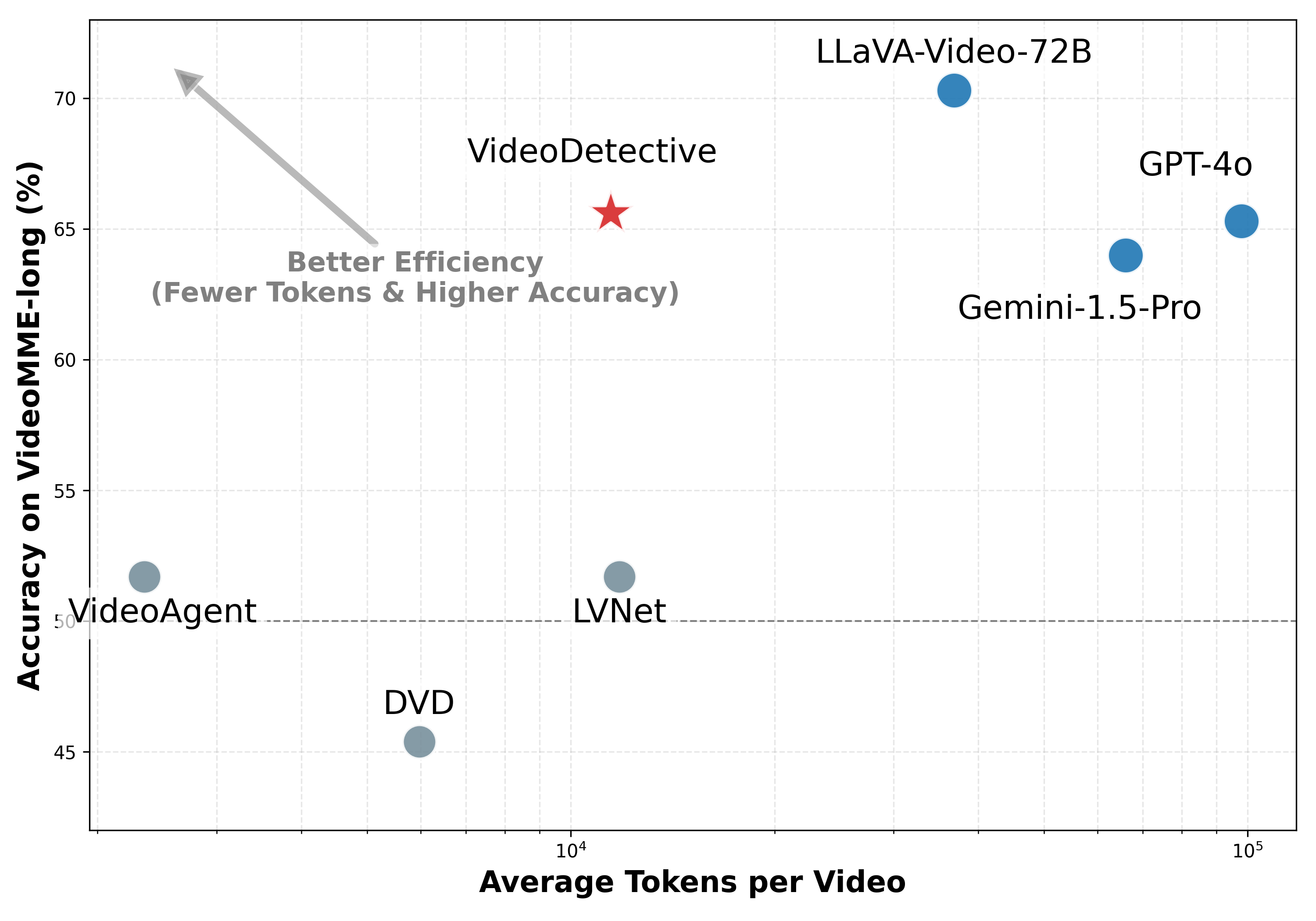
As shown in Figure 3, we report the average token consumption per video on VideoMME-long and compare VideoDetective with both model and method baselines.

Token Efficiency Analysis. As illustrated in Figure 3, VideoDetective achieves the highest token efficiency among all compared methods. Specifically, VideoDetective attains competitive accuracy (65.6%) with moderate token consumption ($\sim$10k per video), demonstrating superior cost-effectiveness compared to both model baselines and method baselines. In comparison, proprietary models such as GPT-4o (65.3%, $\sim$10⁵ tokens) and Gemini-1.5-Pro (64.2%, $\sim$10⁵ tokens) achieve comparable accuracy but require approximately 10$\times$ more tokens. Among method baselines, although VideoAgent, DVD, and LVNet have lower token consumption ($\sim$10⁴ tokens), their accuracy is significantly limited ($<$52%). This demonstrates that VideoDetective achieves the optimal position on the efficiency-accuracy Pareto frontier by strategically investing computational resources into high-value active inference.

5 Conclusion

We present VideoDetective, an inference framework that integrates both extrinsic query relevance and intrinsic video correlations. By modeling a long video as a visual–temporal affinity graph and performing a hypothesis–verification–refinement inference loop, we propagate query-relevance signals from sparse local observations to the entire video, thereby locating critical clues for long-video question answering. Extensive experiments on four challenging benchmarks demonstrate that our approach achieves competitive performance against strong MLLMs and consistently outperforms existing baselines, while maintaining computational efficiency through sparse sampling.

Limitation. Our method relies on the self-reflection capability of VLMs to provide feedback signals (e.g., “missing keywords”); future work may explore more sophisticated relevance assessment mechanisms for improved robustness.

Appendix A Example Figure

See Fig. 4 for an example.

Figure 4: An example of VideoDetective

Appendix B Belief Propagation: Theoretical Analysis

B.1 Closed-form Solution

The iterative diffusion process in Eq. (13) converges to a closed-form solution. After infinite iterations, the belief field converges to: $\boldsymbol{F}^{\star}=(1-\beta)\left(\mathbf{I}-\beta\,\mathbf{W}_{\mathrm{norm}}\right)^{-1}\boldsymbol{Y},$ where $\mathbf{I}$ is the identity matrix. This can be derived by setting $\boldsymbol{F}^{(t+1)}=\boldsymbol{F}^{(t)}=\boldsymbol{F}^{\star}$ and solving for $\boldsymbol{F}^{\star}$.

B.2 Convergence Analysis

The spectral radius of the symmetric normalized affinity matrix $\mathbf{W}_{\mathrm{norm}}$ is bounded by 1 due to the normalization in Eq. (3). This ensures that the iterative process converges exponentially fast. Specifically, let $\lambda_{\max}$ denote the largest eigenvalue of $\mathbf{W}_{\mathrm{norm}}$. The convergence rate is determined by $\beta\lambda_{\max}<1$, which guarantees stability.

B.3 Computational Efficiency

Direct matrix inversion to obtain the closed-form solution requires $O(K^{3})$ operations. In contrast, with top-$k$ sparsification and sparse matrix-vector multiplication, the iterative approach requires $O(TKk)$ operations, where $T$ is the number of iterations (typically $T\ll K$ and $k\ll K$). If implemented with dense matrix operations, the cost becomes the looser $O(TK^{2})$ upper bound. More importantly, when a new observation arrives and updates $\boldsymbol{Y}^{(t)}$, we can continue iterating from the current state $\boldsymbol{F}^{(t)}$ without recomputing from scratch, enabling efficient incremental updates crucial for active learning.

Appendix C Evidence Selection: Detailed Algorithm

C.1 Graph-NMS Algorithm

To avoid selecting redundant evidence from spatially-temporally adjacent segments, we employ a Graph-NMS procedure that suppresses neighbors of already-selected nodes (Alg. 2).

Algorithm 2 Graph-NMS for Evidence Selection

0: Final belief field $\boldsymbol{F}^{(T)}$, prior channels $\{Y^{\mathrm{prior}}_{r}\}_{r=1}^{R}$, affinity matrix $\tilde{\mathbf{W}}$, suppression factor $\eta\in(0,1)$, number of nodes to select $m$

0: Selected node set $\mathcal{S}$

1: Initialize $\mathcal{S}\leftarrow\emptyset$, $\boldsymbol{F}^{\prime}\leftarrow\boldsymbol{F}^{(T)}$

2: // Ensure each facet has at least one representative

3: for $r=1$ to $R$ do

4:  $i_{r}\leftarrow\operatorname*{arg\,max}_{i}(Y^{\mathrm{prior}}_{r})_{i}\cdot F^{\prime}_{i}$

5:  $\mathcal{S}\leftarrow\mathcal{S}\cup\{i_{r}\}$

6: end for

7: // Iteratively select high-confidence nodes

8: while $|\mathcal{S}|<m$ do

9:  $i^{\star}\leftarrow\operatorname*{arg\,max}_{i\notin\mathcal{S}}F^{\prime}_{i}$

10:  if $F^{\prime}_{i^{\star}}\leq 0$ then

11:   break {No more positive confidence nodes}

12:  end if

13:  $\mathcal{S}\leftarrow\mathcal{S}\cup\{i^{\star}\}$

14:  // Suppress neighbors

15:  for each neighbor $j\in\mathcal{N}(i^{\star})$ with $\tilde{W}_{i^{\star}j}>0$ do

16:   $F^{\prime}_{j}\leftarrow\eta\cdot F^{\prime}_{j}$

17:  end for

18: end while

19: return $\mathcal{S}$

The suppression factor $\eta$ controls the strength of neighbor suppression. A smaller $\eta$ leads to more aggressive suppression, encouraging selection of nodes that are more dispersed in the graph. In our experiments, we set $\eta=0.2$.

C.2 Evidence Packaging Details

For each selected node $i\in\mathcal{S}$, we construct a compact multimodal evidence package consisting of:

• Visual frames: Sample $n_{f}$ representative frames uniformly from the time span $[s_{i},e_{i}]$. In practice, we use $n_{f}=4$ for computational efficiency.

• Best textual evidence: Among the three evidence sources (caption $e_{i}^{\mathrm{cap}}$, OCR text $e_{i}^{\mathrm{ocr}}$, ASR text $e_{i}^{\mathrm{asr}}$), select the one with the highest relevance score computed in §3.3.2:

  $$e_{i}^{\mathrm{best}}=\operatorname*{arg\,max}_{e\in\{e_{i}^{\mathrm{cap}},e_{i}^{\mathrm{ocr}},e_{i}^{\mathrm{asr}}\}}\max_{r}s(e,f_{r}).$$ (14)

  This ensures we include only the most relevant textual evidence while avoiding redundancy.

• Temporal information: The start and end timestamps $[s_{i},e_{i}]$ to maintain temporal ordering.

These packages are sorted by temporal order and concatenated into a structured prompt for the downstream MLLM, which generates the final answer based on the aggregated evidence.

Appendix D Prompts for LLM and VLM Calls

This section provides the core prompts used in our implementation.

D.1 Query Decomposition Prompt (LLM)

The LLM decomposes the query into entities (for keyword matching) and events (for semantic matching).

D.2 Observer Inspection Prompt (VLM)

The VLM observes a video segment and generates a caption plus logical gap analysis.

D.3 Final Answer Generation Prompt (VLM) When Evaluating

The VLM generates the final answer based on selected evidence frames.

Appendix E Implementation Details and Hyperparameters

This section provides complete hyperparameter settings used in our experiments. All parameters are consistent across all benchmarks unless otherwise specified.

E.1 Backbone Comparison Experimental Configuration

For the backbone comparison experiments shown in Figure 2, we use the following configurations:

Frame Sampling:

• VideoXL2, Oryx-1.5: 16 frames

• InternVL-2.5: 8 frames

• All other models: 32 frames

LLM configuration:

• GLM, SeedVL, and Qwen3-VL (30B/32B variants): Qwen3-30B as the LLM planner

• All other models: Qwen3-8B as the LLM planner

These configurations ensure that each model is tested under its optimal or commonly used settings while maintaining fairness in comparison. The varying frame sampling reflect the different input capacity and design of each model, and the LLM selection is matched to the scale of the visual backbone for computational efficiency.

E.2 Main Results Table Configuration

For the main comparison results shown in Table 2, we instantiate VideoDetective with two configurations to demonstrate its effectiveness across different parameter scales:

Lightweight Setting ($<$30B):

• Visual-Language Model (VLM): Qwen3-VL-8B-Instruct

• Language Model (LLM) Planner: Qwen3-8B-Instruct

• Final answer frame sampling: 32 frames

Larger-scale Setting ($\geq$30B):

• Visual-Language Model (VLM): SeedVL-1.5

• Language Model (LLM) Planner: Qwen3-30B-Instruct

• Final answer frame sampling: 32 frames

Both configurations share the same hyperparameters for graph construction, belief propagation, and active inference as specified in subsequent sections. The frame budget for final answer generation is fixed at 32 frames across both settings to ensure fair comparison with baseline models.

E.3 Token Efficiency Data Collection

For the token efficiency analysis shown in Figure 3, we report the average token consumption per video on VideoMME-long. The data is collected through the following methods:

Experimental Measurements (Method Baselines):

• VideoAgent, DVD, LVNet, and VideoDetective: The token counts are directly obtained from real experimental runs via API response data. These values represent the actual token consumption during inference.

Estimated Lower Bounds (Model Baselines):

• Gemini-1.5-Pro, GPT-4o, and LLaVA-Video-72B: We estimate the lower bound of token consumption based on:

  1. Official sampling rates (frames per video)

  2. Per-frame token counts specified in official API documentation

  3. Standard video resolution settings

Important Notes:

• These estimates include only image tokens and exclude text prompts, system instructions, and other textual overhead.

• This makes them conservative baselines—the actual token consumption of these models would be higher in practice.

• All measurements are averaged across all videos in the VideoMME-long benchmark.

E.4 Lexical and Semantic Similarity Computation

We provide detailed implementation of the lexical and semantic similarity scores used in evidence scoring (§3.3.2).

E.4.1 Motivation: Complementary Sparse-Dense Retrieval

Sparse retrieval (lexical matching) and dense retrieval (semantic matching) provide complementary inductive biases (Robertson et al., 2009; Karpukhin et al., 2020):

• Dense vectors (embeddings): Excel at handling synonym paraphrasing and semantic equivalence (e.g., ”automobile” $\approx$ ”car”), enabling robust generalization. However, they are susceptible to “semantic drift”—embeddings may conflate related but distinct concepts, leading to false positives (high recall, lower precision).

• Sparse lexical matching (IDF-weighted overlap): Ensure symbol-level precision by exact token matching (e.g., distinguishing ”bank” as financial institution vs. riverbank). However, it is insensitive to paraphrasing and synonyms (high precision, low recall). This score is TF-IDF-inspired but does not require constructing full TF-IDF vectors.

By combining both approaches with source-aware weighting (§3.3.1), we achieve both precision and recall: lexical matching captures exact mentions while semantic matching handles variations and implicit references.

E.4.2 IDF-weighted Lexical Overlap (Sparse Matching)

For lexical matching, we use an IDF-weighted lexical overlap score with standard preprocessing:

1. Text preprocessing: Lowercase conversion, stopword removal, and lemmatization.

2. IDF computation: Pre-computed on a large corpus, with out-of-vocabulary words assigned a default IDF value.

3. Score computation: For evidence text $e$ and keyword set $\mathcal{K}_{r}$:

   $$s_{\mathrm{lex}}(e,f_{r})=\min\left(1.0,\frac{\sum_{t\in e\cap\mathcal{K}_{r}}\text{IDF}(t)}{Z_{\mathrm{lex}}}\right)$$

   where $Z_{\mathrm{lex}}=3.0$ is a normalization constant.

4. Normalization: We clip scores to $[0,1]$ via the $\min(\cdot)$ term above.

E.4.3 Embedding-based Semantic Similarity

For semantic matching, we use SigLIP text encoder with cosine similarity:

1. Text encoding: $\psi(e)=\text{SigLIP-Text}(e)\in\mathbb{R}^{d}$, $\|\psi(e)\|_{2}=1$.

2. Score computation: For evidence text $e$ and semantic query set $\mathcal{P}_{r}$, we compute:

   $$s_{\mathrm{sem}}(e,f_{r})=\max_{p\in\mathcal{P}_{r}}\langle\psi(e),\psi(p)\rangle$$

   where $p$ represents semantic queries (event descriptions) that capture the contextual meaning of each facet.

3. Batch encoding: All semantic queries are pre-encoded for efficiency.

E.5 Source-aware Fusion

Different evidence sources have different signal-to-noise characteristics:

• OCR text: High precision, low recall. Weight: $\lambda_{\mathrm{ocr}}=0.7$ (trust lexical more).

  $$s_{\mathrm{ocr}}(e,f_{r})=0.7\cdot s_{\mathrm{lex}}(e,f_{r})+0.3\cdot s_{\mathrm{sem}}(e,f_{r})$$

• ASR text: Balanced. Weight: $\lambda_{\mathrm{asr}}=0.5$ (equal trust).

  $$s_{\mathrm{asr}}(e,f_{r})=0.5\cdot s_{\mathrm{lex}}(e,f_{r})+0.5\cdot s_{\mathrm{sem}}(e,f_{r})$$

• Caption: High recall, may generalize. Weight: $\lambda_{\mathrm{cap}}=0.3$ (trust semantic more).

  $$s_{\mathrm{cap}}(e,f_{r})=0.3\cdot s_{\mathrm{lex}}(e,f_{r})+0.7\cdot s_{\mathrm{sem}}(e,f_{r})$$

Final node score: $s_{i}=\max_{e\in E_{i},\,r}s(e,f_{r})$.

E.5.1 Event Description Generation for Semantic Channel

This section details how the event descriptions $\{e_{i}\}$ are generated, which are used in the Hypothesis stage (§3.3) for multi-route prior initialization. Specifically, in Eq. (5), the semantic query $p\in\mathcal{P}_{r}$ is matched against these event descriptions to compute the semantic channel of the prior score.

Generation process:

1. Uniform sampling: Extract $F$ frames uniformly distributed across the entire video (not per-node). We reuse the same frame sampling number $F$ as the final answer generation.

2. VLM generation (time-stamped event timeline): Use the VLM to generate a coarse event timeline based on these $F$ frames, capturing the overall narrative and key events. Concretely, the VLM outputs a list of event items, each with an approximate temporal span (e.g., start/end timestamps or the corresponding frame indices among the $F$ sampled frames) plus a short textual description.

3. Deterministic node-level assignment: Each node corresponds to a video chunk with a temporal interval $[s_{i},e_{i}]$. We assign to node $i$ all event items whose temporal spans overlap with $[s_{i},e_{i}]$ (or whose associated sampled-frame indices fall within the node’s interval), and concatenate their descriptions to form $e_{i}$. If no event item overlaps, we assign the temporally nearest event item (by midpoint distance) as $e_{i}$.

Important notes:

• This event description is coarse-grained and serves as a semantic complement to the keyword-based (cross-modal) channel in the multi-route prior.

• It helps capture high-level event semantics that pure keyword matching may miss (e.g., “A person explains X before demonstrating Y”).

• In practice, we set skeleton_frames=$F$ and use the same VLM backbone for consistency.

E.6 Graph Construction and Propagation

Table 5: Graph construction and belief propagation parameters.

Parameter	Symbol	Value
Visual-temporal fusion weight	$\alpha$	0.6
Temporal decay factor	$\tau$	30.0
Top-$k$ sparsification	$k$	8
Scene boundary threshold	$\theta_{\mathrm{sim}}$	0.82
Minimum chunk length	$L_{\min}$	10 frames
Propagation iterations	$T_{\mathrm{prop}}$	7
Diffusion smoothness parameter	$\beta$	0.6

E.7 Active Inference and Observation

Table 6: Active inference and observation parameters.

Parameter	Symbol	Value
Final answer frame sampling	$F$	32 frames
Base max steps	–	10
Steps per extra option	–	1
Local observation window	–	9 frames
Retry relevance threshold	–	0.2
Fallback max relevance threshold	–	0.4
Fallback mean relevance threshold	–	0.2
Flat gap threshold	–	0.15
Multi-route fusion weight	$\alpha_{\mathrm{route}}$	0.5

E.8 Evidence Selection and Scoring

Table 7: Evidence selection and scoring parameters.

Parameter	Symbol	Value
Number of chunks to select	$m$	8
Frames per chunk	$n_{f}$	4
Minimum uniform frames	–	4
Graph-NMS suppression factor	$\eta$	0.2
Frame deduplication threshold	–	0.92
Relaxed deduplication threshold	–	0.95
Fallback similarity threshold	–	0.90
Source-aware fusion weights
OCR text weight	$\lambda_{\mathrm{ocr}}$	0.7 (lex) + 0.3 (sem)
ASR text weight	$\lambda_{\mathrm{asr}}$	0.5 (lex) + 0.5 (sem)
Caption weight	$\lambda_{\mathrm{cap}}$	0.3 (lex) + 0.7 (sem)
Lexical normalization constant	$Z_{\mathrm{lex}}$	3.0 (clip to [0,1])

E.9 Model Configuration

Table 8: Model configurations for main experiments (Qwen3-30B + SeedVL-1.5).

Component	Configuration
Visual-Language Model (VLM)
Model	SeedVL-1.5
Max tokens	4096
Temperature	0.0
Timeout	300s
Text Language Model (LLM)
Model	Qwen3-30B-Instruct
Max tokens	2048
Temperature	0.0
Visual Encoder
Image encoder	SigLIP-SO400M-patch14-384
Text encoder	SigLIP (text tower)
Max text length	64 tokens
Evidence Extraction Tools
VLM caption	SeedVL-1.5 (visual description)
OCR extraction	EasyOCR (on-screen text)
ASR transcription	Whisper (speech-to-text)
Preprocessing
Sampling rate	1.0 FPS
Cache enabled	Yes

Multi-source evidence generation: During observation of node $i$, we extract three complementary evidence sources: (1) VLM caption: the VLM generates a textual description of the visual content in sampled frames; (2) OCR text: EasyOCR extracts any on-screen text visible in the frames; (3) ASR transcript: Whisper provides pre-generated speech transcripts for the corresponding time segment. These three sources are scored independently via lexical-semantic matching (§3.3.1), and the maximum score is used as the node’s relevance: $s_{i}=\max\{s_{\mathrm{ocr}},s_{\mathrm{asr}},s_{\mathrm{cap}}\}$.

E.10 Retry and Error Handling

Table 9: Retry mechanism parameters for API calls.

Parameter	Value
Max retry attempts	5
Base retry delay	1.0s
Max retry delay	20.0s

References

- Achiam et al. (2023) Achiam, J., Adler, S., Agarwal, S., Ahmad, L., Akkaya, I., Aleman, F. L., Almeida, D., Altenschmidt, J., Altman, S., Anadkat, S., et al. Gpt-4 technical report. arXiv preprint arXiv:2303.08774, 2023.
- Arivazhagan et al. (2023) Arivazhagan, M. G., Liu, L., Qi, P., Chen, X., Wang, W. Y., and Huang, Z. Hybrid hierarchical retrieval for open-domain question answering. In Findings of ACL 2023, 2023.
- Awasthi et al. (2022) Awasthi, N., Vermeer, L., Fixsen, L. S., Lopata, R. G., and Pluim, J. P. Lvnet: Lightweight model for left ventricle segmentation for short axis views in echocardiographic imaging. IEEE Trans. Ultrason., Ferroelectr., Freq. Control, 69(6), 2022.
- Bai et al. (2025a) Bai, S., Cai, Y., Chen, R., Chen, K., Chen, X., et al. Qwen3-VL Technical Report. arXiv preprint arXiv:2511.21631, 2025a.
- Bai et al. (2025b) Bai, S., Chen, K., Liu, X., Wang, J., Ge, W., Song, S., Dang, K., Wang, P., Wang, S., Tang, J., et al. Qwen2. 5-vl technical report. arXiv preprint arXiv:2502.13923, 2025b.
- Belkin & Niyogi (2003) Belkin, M. and Niyogi, P. Laplacian eigenmaps for dimensionality reduction and data representation. Neural computation, 15(6), 2003.
- Belkin et al. (2006) Belkin, M., Niyogi, P., and Sindhwani, V. Manifold regularization: A geometric framework for learning from labeled and unlabeled examples. Journal of machine learning research, 7(11), 2006.
- Bodla et al. (2017) Bodla, N., Singh, B., Chellappa, R., and Davis, L. S. Soft-nms–improving object detection with one line of code. In ICCV, 2017.
- Chen et al. (2024a) Chen, Y., Xue, F., Li, D., Hu, Q., Zhu, L., Li, X., Fang, Y., Tang, H., Yang, S., Liu, Z., et al. Longvila: Scaling long-context visual language models for long videos. arXiv preprint arXiv:2408.10188, 2024a.
- Chen et al. (2025) Chen, Y., Huang, W., Shi, B., Hu, Q., Ye, H., Zhu, L., Liu, Z., Molchanov, P., Kautz, J., Qi, X., et al. Scaling rl to long videos. arXiv preprint arXiv:2507.07966, 2025.
- Chen et al. (2024b) Chen, Z., Wang, W., Cao, Y., Liu, Y., Gao, Z., Cui, E., Zhu, J., Ye, S., Tian, H., Liu, Z., et al. Expanding performance boundaries of open-source multimodal models with model, data, and test-time scaling. arXiv preprint arXiv:2412.05271, 2024b.
- Chung (1997) Chung, F. R. K. Spectral Graph Theory, volume 92 of CBMS Regional Conference Series in Mathematics. American Mathematical Society, 1997. ISBN 978-0-8218-0315-8. doi: 10.1090/cbms/092.
- Comanici et al. (2025) Comanici, G., Bieber, E., Schaekermann, M., Pasupat, I., Sachdeva, N., Dhillon, I., Blistein, M., Ram, O., Zhang, D., Rosen, E., et al. Gemini 2.5: Pushing the frontier with advanced reasoning, multimodality, long context, and next generation agentic capabilities. arXiv preprint arXiv:2507.06261, 2025.
- Fan et al. (2024) Fan, Y., Ma, X., Wu, R., Du, Y., Li, J., Gao, Z., and Li, Q. Videoagent: A memory-augmented multimodal agent for video understanding. In ECCV, 2024.
- Fu et al. (2025a) Fu, C., Dai, Y., Luo, Y., Li, L., Ren, S., Zhang, R., Wang, Z., Zhou, C., Shen, Y., Zhang, M., et al. Video-mme: The first-ever comprehensive evaluation benchmark of multi-modal llms in video analysis. In CVPR, 2025a.
- Fu et al. (2025b) Fu, C., Lin, H., Wang, X., Zhang, Y.-F., Shen, Y., Liu, X., Cao, H., Long, Z., Gao, H., Li, K., et al. Vita-1.5: Towards gpt-4o level real-time vision and speech interaction. arXiv preprint arXiv:2501.01957, 2025b.
- Guo et al. (2025) Guo, D., Wu, F., Zhu, F., Leng, F., Shi, G., Chen, H., Fan, H., Wang, J., Jiang, J., Wang, J., et al. Seed1. 5-vl technical report. arXiv preprint arXiv:2505.07062, 2025.
- Hong et al. (2025) Hong, W., Yu, W., Gu, X., Wang, G., Gan, G., Tang, H., Cheng, J., Qi, J., Ji, J., Pan, L., et al. Glm-4.1 v-thinking: Towards versatile multimodal reasoning with scalable reinforcement learning. arXiv preprint arXiv:2507.01006, 2025.
- Hurst et al. (2024) Hurst, A., Lerer, A., Goucher, A. P., Perelman, A., Ramesh, A., Clark, A., Ostrow, A., Welihinda, A., Hayes, A., Radford, A., et al. Gpt-4o system card. arXiv preprint arXiv:2410.21276, 2024.
- JaidedAI (2023) JaidedAI. Easyocr. https://github.com/JaidedAI/EasyOCR, 2023. Accessed: 2026-01-21.
- Jeong et al. (2025) Jeong, S., Kim, K., Baek, J., and Hwang, S. J. Videorag: Retrieval-augmented generation over video corpus. arXiv preprint arXiv:2501.05874, 2025.
- Karpukhin et al. (2020) Karpukhin, V., Oguz, B., Min, S., Lewis, P. S., Wu, L., Edunov, S., Chen, D., and Yih, W.-t. Dense passage retrieval for open-domain question answering. In EMNLP, 2020.
- Kipf (2016) Kipf, T. Semi-supervised classification with graph convolutional networks. arXiv preprint arXiv:1609.02907, 2016.
- Li et al. (2024) Li, B., Zhang, Y., Guo, D., Zhang, R., Li, F., Zhang, H., Zhang, K., Zhang, P., Li, Y., Liu, Z., et al. Llava-onevision: Easy visual task transfer. arXiv preprint arXiv:2408.03326, 2024.
- Li et al. (2018) Li, Q., Han, Z., and Wu, X.-M. Deeper insights into graph convolutional networks for semi-supervised learning. In AAAI, volume 32, 2018.
- Lin et al. (2024) Lin, B., Ye, Y., Zhu, B., Cui, J., Ning, M., Jin, P., and Yuan, L. Video-llava: Learning united visual representation by alignment before projection. In EMNLP, 2024.
- Liu et al. (2024a) Liu, A., Feng, B., Xue, B., Wang, B., Wu, B., Lu, C., Zhao, C., Deng, C., Zhang, C., Ruan, C., et al. Deepseek-v3 technical report. arXiv preprint arXiv:2412.19437, 2024a.
- Liu et al. (2025) Liu, J., Wang, Y., Zhang, L., et al. Towards training-free long video understanding: methods, benchmarks, and open challenges. Vicinagearth, 2(6), 2025. doi: 10.1007/s44336-025-00017-w.
- Liu et al. (2024b) Liu, Z., Dong, Y., Liu, Z., Hu, W., Lu, J., and Rao, Y. Oryx mllm: On-demand spatial-temporal understanding at arbitrary resolution. arXiv preprint arXiv:2409.12961, 2024b.
- Luo et al. (2024) Luo, Y., Zheng, X., Li, G., Yin, S., Lin, H., Fu, C., Huang, J., Ji, J., Chao, F., Luo, J., et al. Video-rag: Visually-aligned retrieval-augmented long video comprehension. arXiv preprint arXiv:2411.13093, 2024.
- Qin et al. (2025) Qin, M., Liu, X., Liang, Z., Shu, Y., Yuan, H., Zhou, J., Xiao, S., Zhao, B., and Liu, Z. Video-xl-2: Towards very long-video understanding through task-aware kv sparsification. arXiv preprint arXiv:2506.19225, 2025.
- Radford et al. (2021) Radford, A., Kim, J. W., Hallacy, C., Ramesh, A., Goh, G., Agarwal, S., Sastry, G., Askell, A., Mishkin, P., Clark, J., et al. Learning transferable visual models from natural language supervision. In ICML. PmLR, 2021.
- Radford et al. (2023) Radford, A., Kim, J. W., Xu, T., Brockman, G., McLeavey, C., and Sutskever, I. Robust speech recognition via large-scale weak supervision. In ICML, 2023.
- Robertson et al. (2009) Robertson, S., Zaragoza, H., et al. The probabilistic relevance framework: Bm25 and beyond. Foundations and trends® in information retrieval, 3(4), 2009.
- Shen et al. (2024) Shen, X., Xiong, Y., Zhao, C., Wu, L., Chen, J., Zhu, C., Liu, Z., Xiao, F., Varadarajan, B., Bordes, F., et al. Longvu: Spatiotemporal adaptive compression for long video-language understanding. arXiv preprint arXiv:2410.17434, 2024.
- Shen et al. (2025) Shen, Y., Fu, C., Dong, S., Wang, X., Zhang, Y.-F., Chen, P., Zhang, M., Cao, H., Li, K., Lin, S., et al. Long-vita: Scaling large multi-modal models to 1 million tokens with leading short-context accuracy. arXiv preprint arXiv:2502.05177, 2025.
- Shu et al. (2025) Shu, Y., Liu, Z., Zhang, P., Qin, M., Zhou, J., Liang, Z., Huang, T., and Zhao, B. Video-xl: Extra-long vision language model for hour-scale video understanding. In CVPR, 2025.
- Tang et al. (2025) Tang, X., Qiu, J., Xie, L., Tian, Y., Jiao, J., and Ye, Q. Adaptive keyframe sampling for long video understanding. In CVPR, 2025.
- Tao et al. (2025) Tao, K., Qin, C., You, H., Sui, Y., and Wang, H. Dycoke: Dynamic compression of tokens for fast video large language models. In CVPR, 2025.
- Team et al. (2024) Team, G., Georgiev, P., Lei, V. I., Burnell, R., Bai, L., Gulati, A., Tanzer, G., Vincent, D., Pan, Z., Wang, S., et al. Gemini 1.5: Unlocking multimodal understanding across millions of tokens of context. arXiv preprint arXiv:2403.05530, 2024.
- Wang et al. (2025a) Wang, P., Song, S., Ji, H., Cao, S., Yu, H., Liu, Z., et al. From models to systems: A comprehensive survey of efficient multimodal learning. Authorea Preprints, 2025a.
- Wang et al. (2025b) Wang, W., He, Z., Hong, W., Cheng, Y., Zhang, X., Qi, J., Ding, M., Gu, X., Huang, S., Xu, B., et al. Lvbench: An extreme long video understanding benchmark. In ICCV, 2025b.
- Wang et al. (2024) Wang, X., Zhang, Y., Zohar, O., and Yeung-Levy, S. Videoagent: Long-form video understanding with large language model as agent. In ECCV, 2024.
- Wang et al. (2025c) Wang, X., Si, Q., Zhu, S., Wu, J., Cao, L., and Nie, L. Adaretake: Adaptive redundancy reduction to perceive longer for video-language understanding. In Findings of ACL 2025, 2025c.
- Wang et al. (2025d) Wang, Z., Zhou, H., Wang, S., Li, J., Xiong, C., Savarese, S., Bansal, M., Ryoo, M. S., and Niebles, J. C. Active video perception: Iterative evidence seeking for agentic long video understanding. arXiv preprint arXiv:2512.05774, 2025d.
- Wu et al. (2024) Wu, H., Li, D., Chen, B., and Li, J. Longvideobench: A benchmark for long-context interleaved video-language understanding. In NeurIPS, 2024.
- Yang et al. (2025) Yang, A., Li, A., Yang, B., Zhang, B., Hui, B., Zheng, B., Yu, B., Gao, C., Huang, C., Lv, C., et al. Qwen3 technical report. arXiv preprint arXiv:2505.09388, 2025.
- Yedidia et al. (2003) Yedidia, J. S., Freeman, W. T., Weiss, Y., et al. Understanding belief propagation and its generalizations. Exploring artificial intelligence in the new millennium, 8(236-239), 2003.
- Yuan et al. (2025) Yuan, H., Liu, Z., Zhou, J., Wen, J.-R., and Dou, Z. Videodeepresearch: Long video understanding with agentic tool using. arXiv preprint arXiv:2506.10821, 2025.
- Zhai et al. (2023) Zhai, X., Mustafa, B., Kolesnikov, A., and Beyer, L. Sigmoid loss for language image pre-training. In ICCV, 2023.
- Zhang et al. (2024a) Zhang, P., Zhang, K., Li, B., Zeng, G., Yang, J., Zhang, Y., Wang, Z., Tan, H., Li, C., and Liu, Z. Long context transfer from language to vision. arXiv preprint arXiv:2406.16852, 2024a.
- Zhang et al. (2025) Zhang, X., Jia, Z., Guo, Z., Li, J., Li, B., Li, H., and Lu, Y. Deep video discovery: Agentic search with tool use for long-form video understanding. arXiv preprint arXiv:2505.18079, 2025.
- Zhang et al. (2024b) Zhang, Y., Wu, J., Li, W., Li, B., Ma, Z., Liu, Z., and Li, C. Video instruction tuning with synthetic data. arXiv preprint arXiv:2410.02713, 2024b.
- Zhi et al. (2025) Zhi, Z., Wu, Q., Li, W., Li, Y., Shao, K., Zhou, K., et al. Videoagent2: Enhancing the llm-based agent system for long-form video understanding by uncertainty-aware cot. arXiv preprint arXiv:2504.04471, 2025.
- Zhou et al. (2004) Zhou, D., Bousquet, O., Lal, T. N., Weston, J., and Schölkopf, B. Learning with local and global consistency. In NeurIPS, volume 16, 2004.
- Zhou et al. (2025) Zhou, J., Shu, Y., Zhao, B., Wu, B., Liang, Z., Xiao, S., Qin, M., Yang, X., Xiong, Y., Zhang, B., et al. Mlvu: Benchmarking multi-task long video understanding. In CVPR, 2025.