Risk-Averse Stochastic Assignment on Uncertain Networks

Risk-Averse Stochastic User Equilibrium on Uncertain Transportation Networks

Wencheng Bao, M.Sc. Department of Civil and Environment Engineering, University of Illinois Urbana-Champaign Chrysafis Vogiatzis, Ph.D. Department of Industrial and Enterprise Systems Engineering, University of Illinois Urbana-Champaign Eleftheria Kontou, Ph.D.* Department of Civil and Environment Engineering, University of Illinois Urbana-Champaign, Corresponding author: kontou@illinois.edu Extreme weather events, like flooding, disrupt urban transportation networks by reducing speeds and capacities, and by closing roadways. These hazards create regime-dependent uncertainty in link performance and travel-time distribution tails, challenging conventional traffic assignment that relies on the expectation of cost or mean excess of cost summation. This study develops a risk- and ambiguity-aware traffic assignment framework coupling stochastic supply driven by hazard impacts, endogenous route choice with choice set truncation, and tail-risk management within a tractable convex truncated stochastic user equilibrium (TSUE) formulation. Travelers’ perceived costs use a normalized mean-CVaR certainty equivalent encoding tail sensitivity into two interpretable parameters ($\alpha$ and $\lambda$) while preserving convexity. We propose two complementary treatments. TSUE-Stochastic Programming (TSUE-SP) optimizes a nominal risk-aware TSUE balancing average performance and adverse-tail outcomes. TSUE-Distributionally Robust Optimization (TSUE-DRO) protects against calibration error and distributional misspecification by incorporating robustness over a $1$-Wasserstein ambiguity set, and when appropriate, over structured regime-dependent sets for piecewise-stationary hazards (non-stationary distribution case). Duality yields a scenario-based second-order cone program solved via Benders cuts. On a stylized grid network representing downtown Chicago, western corridor traffic increases $67.9\%$ with TSUE-SP and $100.9\%$ with TSUE-DRO relative to a baseline not impacted by the hazard. The formulations redistribute flows without large-scale rerouting, illustrating how tail weighting and distributional ambiguity fine-tune rather than subvert equilibrium choices in hazard-prone networks.

Traffic Assignment, Stochastic User Equilibrium, Stochastic Programming, Distributionally Robust Optimization, Hazard Impacts, Risk-Aversion

1 Introduction

Hazards induced by natural phenomena or anthropogenic activities often disrupt infrastructure systems and their operations, including transportation networks. Flooding affecting major thoroughfares can cause limited and delayed access to employment, educational functions, and health and emergency services (Lightbody 2017). In a modeled 100-year urban flood for 2564 cities in 177 countries across the world, approximately 15% of road kilometers were inundated. Among trips that remain feasible, the average route becomes about 1.5 km longer and 3 minutes slower relative to baseline conditions (He et al. 2022).

Weather-related hazards measurably degrade mobility and road safety. Loren (2024) estimates that 24% of weather-related crashes occur on snowy, slushy, or icy pavement, with another 15% during active snowfall or sleet. Rain, snow, high winds, fog, and hurricanes all elevate crash risk and reduce travel speeds (Dey et al. 2014). In Florida, moderate rainfall decreases average vehicle speeds by roughly 10 mph (Collins and Pietrzyk 2001). These disruptions are consequential for accessibility, safety, and social well-being, and are expected to intensify as infrastructure ages and extreme events become more frequent (Dharmarathne et al. 2024).

Such disruptions typically result in right-skewed, long-tailed travel time distributions (Van Lint et al. 2008, Zang et al. 2022, Li et al. 2018). Risk-neutral assignment, based on expected travel times, can therefore underestimate rare, but severe, delays that can lead to precautionary behavior and choices. To that extent, empirical evidence has consistently pointed to the fact that travelers tend to choose reliable routes rather than routes that are (on average) faster, but more unreliable (Liu et al. 2004, Carrion and Levinson 2012). Hence, capturing the upper tail, through CVaR-type constructs, is essential when hazards can lead to low-probability but high-severity outcomes.

We model travel time as a random variable following any distribution. We focus on risk-averse travelers whose route choices depend on both expected travel time and upper-tail risk (e.g., reliability or quantile measures). A key difficulty is in estimating the distributional parameters, which are necessary for quantifying tail behavior, from noisy and limited observations. This is why our distributionally robust approach that protects against calibration and specification errors can help.

We develop an approach for estimating travel-time distributions under parameter uncertainty. Section 1 introduces current research and challenges. Section 2 provides the problem statement, defines the uncertainty network, and presents the stochastic user equilibrium (SUE) framework. Section 3 summarizes limitations of using only expectation and conditional value at risk (CVaR) in the distribution. Section 4 presents a normalized coupled mean–CVaR certainty equivalent that preserves the scale of deterministic costs. Section 5 introduces a robust, ambiguity-aware equilibrium formulation to hedge against calibration error and distributional misspecification. Section 6 provides a simple example showcasing performance of the proposed structure. Section 7 presents a case study in downtown Chicago, IL to test algorithmic performance.

1.1 Literature overview

SUE leverages a logit choice mechanism to map perceived transport link costs into path selection probabilities. How we quantify each link’s perceived travel time is important for determining link use probabilities and equilibrium flows. When travelers are risk averse, equilibrium in stochastic network settings can still be established under broad conditions (De Palma and Picard 2006, Lianeas et al. 2019, Ordónez and Stier-Moses 2010). In networks affected by hazards, link travel times are random variables rather than deterministic constants. The model must compress a travel time distribution into a behaviorally meaningful reliability-based perceived time that reflects travelers’ aversion to unreliability. Contemporary literature develops and values such reliability and variability measures. These range from scheduling-based reliability premia to additive variability measures and the valuation of travel time variance or reliability, including their interaction with congestion (Batley 2007, Fosgerau and Karlström 2010, Fosgerau and Engelson 2011, Xiao et al. 2017). These reliability-based time constructs directly shape travelers’ perceived link costs and the logit probabilities. This determines the endogenous distribution of flows across links in equilibrium. For example, Chen and Zhou (2010), Chen et al. (2011) define and extend an $\alpha$-reliable mean excess traffic equilibrium model that combines buffer time and tardy time concepts. This explicitly embeds tail delay sensitivity into the equilibrium mechanism, while Nikolova and Stier-Moses (2014) characterize equilibrium under mean-standard deviation objectives and bound efficiency losses for risk-averse commuters.

To characterize risk-averse behavior in hazard-prone networks, the upper tail of the travel time distribution is fundamental. Rare but severe delays dominate perceived disutility and influence equilibrium route choice. Xu et al. (2014) study an $\alpha$-reliable mean excess traffic equilibrium model integrating buffer time and tardy time components beyond a reliability threshold. A parallel stream adopts parametric representations (e.g., lognormal or right-skewed families) to capture tail behavior (Wang and Osaragi 2024, Taylor and others 2012, Kim and Mahmassani 2015). Zang et al. (2024) formalize the tail through an unreliability area, measuring the distribution’s upper tail mass and severity. Their differences represent alternative weights on the unreliability area, reflecting different behavioral emphasis on extreme delays. This enables deriving the value of distribution tail and value of travel time reliability, quantifying willingness to pay to reduce upper tail risk.

However, there are some limitations of existing reliability-based traffic assignment models in hazard-prone networks. First, conventional perceived-cost specifications often summarize stochastic travel time too coarsely to control route reliability. As a result, routes with similar performance can be treated as equally attractive even when they have very different probabilities of exceeding a service threshold, and routes with rare but severe delay realizations may be misrepresented.

Second, if the underlying travel-time distribution is unreliable, biased, or subject to temporal drift, then penalizing tails under a fixed estimated distribution may underestimate the true risk faced by travelers. Moreover, tail-aware route-choice models can introduce substantial parameter sensitivity: nonlinear tail operators, when combined with the exponential truncated-logit kernel, may amplify small changes in tail-related parameters into large shifts in route-choice probabilities and equilibrium flows.

Third, standard reliability-based formulations typically assume that link and route travel times follow fixed stationary distributions, with day-to-day observations treated as independent and identically distributed. In practice, these distributions are estimated from finite data and may be affected by sparse observations, sensor bias, sampling error, or temporal drift. These assumptions become restrictive under nonstationary hazard conditions, such as severe rainstorms, where episodic downpours, drainage cycles, heterogeneous capacity reductions, flooding, hydroplaning, and irregular storm timing can substantially alter travel-time behavior. As a result, historical travel-time distributions may have limited predictive validity for current or future hazardous conditions.

To address these limitations, this paper develops a risk- and ambiguity-aware truncated-logit SUE framework for hazard-prone transportation networks. The framework introduces a normalized risk-sensitive cost aggregation that balances ordinary operating conditions with behaviorally salient upper-tail delay risk, embeds the resulting generalized costs into truncated-logit route choice, and distinguishes path-based and potential-based formulations. The potential-based formulation preserves convex tractability, while the distributionally robust and regime-dependent extensions account for uncertainty in the estimated travel-time law and for hazard regimes with distinct travel-time behavior.

1.2 Our contributions

Our contributions are threefold. First, we formulate a SUE model with scenario-dependent BPR-type link costs. These costs capture hazard-induced changes in free-flow travel time, capacity, congestion amplification, and incident delay, and are embedded in a truncated-logit route-choice structure. We also show why expectation-based route-cost perception is insufficient in hazard-prone networks. Mean travel time may ignore reliability and tail exposure, while pure CVaR may be overly conservative or weakly discriminative under catastrophic disruptions. This motivates a mean-CVaR certainty equivalent.

In addition, we introduce a normalized $(\alpha,\lambda)$-coupled mean-CVaR certainty equivalent. The parameter $\alpha$ identifies the adverse tail, while $\lambda$ governs risk sensitivity through an effective CVaR weight. This construction nests risk neutrality at $\lambda=\alpha$ and supports a stable risk-sensitive truncated-logit model. We then develop three risk-sensitive TSUE formulations. Approach A applies the certainty equivalent directly to path travel times and therefore admits an individual-level behavioral interpretation. Approaches B1 and B2 apply the risk functional to network potential functions, leading to tractable aggregate formulations. We prove that B1 and B2 are equivalent as reduced path-flow optimization problems. Under nondecreasing link travel-time functions and $\theta>0$, entropy regularization renders the reduced B1-B2 objective strictly convex. We also show the B1-B2 optimal path-flow solution is unique. We further establish a theoretical connection between individual risk perception and aggregate equilibrium. Under regime dominance, where all scenarios share a common mild-to-severe ordering across links, the path-based cost in Approach A coincides with the generalized marginal path cost induced by Approach B2. This result provides practical guidance for selecting $\alpha$ and for interpreting the scenario partition induced by $\alpha$. With aligned OD admissibility baselines, the two approaches generate the same truncated-logit choice probabilities and equilibrium flows.

Third, for the potential-based formulations, we develop a $1$-Wasserstein distributionally robust TSUE framework to handle epistemic uncertainty in estimated travel-time distributions. Instead of relying on a single nominal scenario law, the model evaluates the risk-sensitive potential under the worst-case distribution within a Wasserstein ambiguity set, thereby hedging against sampling error, calibration bias, support mismatch, and distributional misspecification. We further extend this formulation to piecewise stationary hazard environments by constructing structured, regime-dependent ambiguity sets, which separate within-regime uncertainty from between-regime shifts. The resulting TSUE-DRO model admits tractable dual, conic, and exchange-based reformulations, and produces equilibrium flows that are more stable under sparse data and nonstationary weather regimes.

2 Problem setting

Let $G=(V,E)$ denote a directed transportation network, where $V$ is the set of nodes and $E$ the set of links. Each link $a\in E$ is assigned a probability signaling whether it can be traversed (open) or not (closed). Assuming link $a\in E$ is traversable, then it will operate under one of a series of mutually exclusive scenarios $\xi_{a}\in\{1,\ldots,S\}$: operating at habitual conditions, at reduced capacity due to hazardous events, or at increased congestion. Each scenario $s$ is associated with a probability $p_{a}^{s}=\mathbb{P}\left[\xi_{a}=s\right]$, with the parameters of the link depending on the scenario. The mathematical notation, including network modeling details, set definitions, decision variables, and other parameters can be found in Appendix A.

2.1 Stochastic travel time function

It is common to represent the link travel time on a transportation network with an extended Bureau of Public Roads (BPR) function (Sheffi 1984):

$$t_{a}\!\bigl(x_{a},\xi_{a}\bigr)\;=\;t_{a}^{0}(\xi_{a})\!\Bigl[1+\alpha(\xi_{a})\,\bigl(x_{a}/c_{a}(\xi_{a})\bigr)^{\beta(\xi_{a})}\Bigr]\;+\;\Delta_{a}(\xi_{a}),$$ (1)

where $x_{a}$ is the link flow. The scenario-specific parameters $\bigl(t_{a}^{0}(\xi_{a}),\,c_{a}(\xi_{a}),\,\alpha(\xi_{a}),\,\beta(\xi_{a}),\,\Delta_{a}(\xi_{a})\bigr)$ and their probabilities are $p_{a}^{s}:=\mathbb{P}[\xi_{a}=s]$.

Following (Lam et al. 2013), rainfall intensity reduces free-flow speed, speed-at-capacity, and maximum flow capacity. Since the BPR coefficients $\alpha$ and $\beta$ are empirical calibration parameters rather than fixed physical constants, scenario-specific values $(\alpha_{s},\beta_{s})$ must be recalibrated to capture regime-dependent changes in link performance. Alternatively, one may retain the baseline $(\alpha,\beta)$ (e.g., (0.15, 4)) and represent weather effects through scenario-dependent free-flow travel times and/or capacity multipliers. Moreover, $\Delta_{a}(\xi_{a})$ represents the additional delay induced by hazard impacts, and thus it is expected to vary with hazard intensity and operating conditions.

For every scenario $s$, the equation 1 is continuously differentiable, strictly increasing, and convex in $x_{a}$ whenever $\beta_{s}\geq 1$. Because expectation is a convex combination of these functions, the expectation inherits monotonicity and convexity. Hence, the cost structure for the user equilibrium (UE) model is maintained, while also explicitly captures (i) free-flow speed changes, (ii) capacity reduction, (iii) congestion amplification, and (iv) fixed incident delays $\Delta_{a,s}$.

2.2 Entropy-based route choice with a truncated logit

We model traveler route choices under uncertainty using an entropy approach with a truncated logit model. The certainty equivalent travel time for a path $k$ is derived as $\phi\left(t_{k}\right)=\mathbb{E}_{\xi}\left[t_{k}(x,\xi)\right]$, where $t_{k}(x,\xi)=\sum_{a\in k}t_{a}\left(x_{a},\xi_{a}\right)$, with $t_{a}\left(x_{a},\xi_{a}\right)$ given by (1). The utility for path $k$ is: $U_{k}=-\theta\phi\left(t_{k}\right)+\delta_{k}$, using parameter $\theta>0$ as the travel time sensitivity, and $\delta_{k}$ being a random variable following a Gumbel distribution, leading to a logit model’s choice probabilities.

For paths $k$ and $k^{\prime}$, the probability of choosing path $k$ over $k^{\prime}$ is:

$$\operatorname{Pr}\left(U_{k}\geq U_{k^{\prime}}\right)=\left(1+\exp\left[-\theta\left(\phi\left(t_{k^{\prime}}\right)-\phi\left(t_{k}\right)\right)\right]\right)^{-1}.$$ (2)

We consider the truncated logit model proposed by Tan et al. (2024), which assigns zero probability to paths exceeding a threshold:

$$P_{k}^{od}=\frac{\left[\exp\left(-\theta\left(\phi\left(t_{k}^{od}\right)-\pi_{rs}\right)\right)-1\right]_{+}}{\sum_{\ell\in K_{od}}\left[\exp\left(-\theta\left(\phi\left(t_{\ell}^{od}\right)-\pi_{od}\right)\right)-1\right]_{+}}$$ (3)

where $[x]_{+}=\max\{x,0\}$. The derivation is provided in Appendix  B.

2.3 Stochastic user equilibrium formulation

Stochastic optimization offers a principled approach to hedge against the uncertainty that hazardous events incur for both link capacities and travel time functions. Due to the above settings, we provide an SP formulation of our problem. The SUE with a truncated logit (TSUE) formulation is integrated with chance constraints to ensure that only reliable paths are considered. The mathematical formulation is shown in (4a)–(4d).

$$\min_{f,v},\quad \mathbb{E}\!\left[Z(f,\xi)\right],\quad Z(f,\xi)=\sum_{a\in A}\int_{0}^{x_{a}}t_{a}(\omega,\xi)\,\mathrm{d}\omega+\frac{1}{\theta}\sum_{o,d}\sum_{k\in K_{od}}\Big[\big(f_{k}^{od}+1\big)\ln\big(f_{k}^{od}+1\big)-f_{k}^{od}\Big]$$ (4a)

s.t. $$\sum_{k\in K_{od}}f_{k}^{od}=q_{od},\quad\forall(o,d)$$ (4b)

$$x_{a}=\sum_{o,d}\sum_{k\in K_{od}}f_{k}^{od}\,\delta_{a,k}^{od},\quad\forall a\in A$$ (4c)

$$f_{k}^{od}\geq 0,\quad\forall(o,d),\ k\in K_{od};\qquad x_{a}\geq 0,\quad\forall a\in A$$ (4d)

where $\delta_{a,k}^{od}\in\{0,1\}$ indicates whether route $k$ uses link $a$.

The objective minimizes the expected total travel time (first term) and includes an entropy term (second term) to reflect stochastic route choices, which is a standard practice in SUE models (Fisk 1980). Flow conservation in (4b) ensures that all OD demand is met. Link flow definitions in (4c) aggregate route flows to link flows. Nonnegativity variable restrictions are in (4d). The formulation is consistent with a TSUE with chance constraints. Let us discuss the convexity of the objective function.

Proposition 2.1

The objective function in (4a) is convex and has a unique path flow solution.

Proof 2.2

Proof. The proof can be found in Appendix C

3 Risk-sensitive cost aggregation

3.1 Limitations of expectation-based path cost aggregation

Let $t_{k}^{od}(v,\xi):=\sum_{a\in k}t_{a}(x_{a},\xi_{a})$ denote the random travel time on path $k\in K_{od}$ under network state $\xi$ (e.g., precipitation, limited visibility, etc.). A standard risk-neutral choice sets the deterministic utility to the mean, $\phi_{k}^{od}(v):=\mathbb{E}_{\xi}\!\left[t_{k}^{od}(v,\xi)\right]$, which is analytically convenient (e.g., preserves convexity of the Beckmann potential, defined as $\sum_{a\in A}\int_{0}^{x_{a}}t_{a}(\omega)\,\mathrm{d}\omega$, a convex transportation network objective whose minimizer corresponds to the UE link flows when link travel times $t_{a}(\cdot)$ are increasing) but can be misleading under rare and highly disruptive hazards.

However, the mean does not control reliability. For any fixed $\pi_{od}$, there exist random travel times $Y$ and $\tilde{Y}$ such that $\mathbb{E}[Y]=\mathbb{E}[\tilde{Y}]$ but $\mathbb{P}(Y>\pi_{od})\neq\mathbb{P}(\tilde{Y}>\pi_{od})$. Hence, a route ranking (or truncation rule) based only on $\mathbb{E}[t_{k}^{od}]$ cannot distinguish routes with identical average performance but different reliability. Furthermore, if transportation network travelers evaluate delay through a nonlinear disutility $u(\cdot)$ (e.g., schedule delay penalties, costs due to missed connections), then the relevant quantity is $\mathbb{E}[u(t_{k}^{od})]$ rather than $u(\mathbb{E}[t_{k}^{od}])$. For convex $u(\cdot)$, Jensen’s inequality yields $u\!\left(\mathbb{E}[t_{k}^{od}]\right)\leq\mathbb{E}\!\left[u(t_{k}^{od})\right]$, so $\phi_{k}^{od}=\mathbb{E}[t_{k}^{od}]$ systematically comes short of penalizing variability and extreme realizations, the effects induced by heavy rain/flooding. Mean feasibility does not imply reliability:

$$\phi_{k}^{od}(v)\leq\pi_{od}\;\;\not\Rightarrow\;\;\mathbb{P}\!\left(t_{k}^{od}(v,\xi)\leq\pi_{od}\right)\geq 1-\eta\quad(\eta\in(0,1)).$$ (5)

Thus, mean-based truncation may still assign nonzero probability to routes that frequently violate service thresholds on days affected by hazards, and may exclude routes with slightly larger means but substantially better reliability. These issues are augmented under regime mixtures. Let $W\in\mathcal{W}:=\{\mathrm{NR},\mathrm{HR},\mathrm{FL}\}$ denote weather regimes, such as normal rain (NR), heavy rain (HR), and flooding (FL). Then, the unconditional mean is decomposed as

$$\mathbb{E}\!\left[t_{k}^{od}\right]=\sum_{w\in\mathcal{W}}\mathbb{P}(W=w)\,\mathbb{E}\!\left[t_{k}^{od}\mid W=w\right].$$ (6)

When travelers have information that $W=\mathrm{FL}$, their travel time valuation is the conditional expectation $\mathbb{E}[t_{k}^{od}\mid W=\mathrm{FL}]$ (or a posterior mean), not the unconditional mean (6).

In the truncated logit model, $\phi_{k}^{od}(v)$ affects path choice in two coupled ways: it defines which paths remain admissible and it determines the relative weights among admissible paths. Since

$$\left[\exp\!\left(-\theta\left(\phi_{k}^{od}(v)-\pi_{od}\right)\right)-1\right]_{+}>0\quad\Longleftrightarrow\quad\phi_{k}^{od}(v)<\pi_{od},$$ (7)

the admissible set implied by mean-based aggregation is $K_{od}^{\mathrm{TL}}(v)=\left\{k\in K_{od}\,\middle|\,\mathbb{E}_{\xi}\!\left[t_{k}^{od}(v,\xi)\right]<\pi_{od}\right\}$.

Moreover, for $k\in K_{od}^{\mathrm{TL}}(v)$, the truncated logit probability depends on $t_{k}^{od}(v,\xi)$ only through its expectation is $P_{k}^{od}(v)\ \propto\ \exp\!\left(-\theta\left(\mathbb{E}_{\xi}[t_{k}^{od}(v,\xi)]-\pi_{od}\right)\right)-1$. So two paths with equal means are treated as equally attractive (up to the Gumbel noise) even if their exceedance probabilities $\mathbb{P}(t_{k}^{od}>\pi_{od})$ differ substantially. The Appendix D gives an example how expectation-based truncation can be misleading in heavy-tailed or mixture settings.

3.2 Conditional value at risk (CVaR) approach and limitation

To address tail risk, we use Conditional Value at Risk (CVaR) as a tail-sensitive alternative for route cost perception. Since travel time distributions are often non-normal (Fosgerau and Fukuda 2012), CVaR is attractive: it requires no distributional assumption and directly quantifies expected loss in the adverse tail. CVaR focuses on the expected losses within the worst $(1-\alpha)$ fraction of scenarios (Rockafellar and Uryasev 2002), is convex, coherent, and has been widely used in hazardous routing and reliability contexts (Toumazis and Kwon 2016, Hosseini and Verma 2018, Li 2019, Su and Kwon 2020). Related travel-time measures include mean excess travel time (METT) and the travel time budget (TTB) (Chen and Zhou 2010), which are analogous to CVaR and VaR, respectively. The limitation is that TTB measures are often non-smooth and may lack favorable convexity properties, and optimizing a single METT (CVaR) level captures only one tail region and may be insensitive to improvements outside that region.

For total travel time (system potential) $Z(f,\xi)$ and confidence level $\alpha\in(0,1)$, CVaR is

$$\operatorname{CVaR}_{\alpha}(Z(f,\xi))=\inf_{\gamma\in\mathbb{R}}\left\{\gamma+\frac{1}{1-\alpha}\mathbb{E}\left[(Z(f,\xi)-\gamma)_{+}\right]\right\},$$ (8)

where $(x)_{+}=\max\{x,0\}$. It is commonly interpreted as the tail conditional mean beyond the $\alpha$-quantile (VaR), $\operatorname{CVaR}_{\alpha}(Z)=\mathbb{E}\!\bigl[\,Z\,\bigm|\,Z\geq\operatorname{VaR}_{\alpha}(Z)\bigr]$.

Figure 1: Illustration of travel-time tail-risk quantification using VaR and CVaR for a non-normal travel-time distribution. The top panel shows the probability density function and marks the mean, the $\alpha$-level VaR (the $\alpha$-quantile), and the corresponding CVaR (the conditional mean travel time given exceedance of VaR). The bottom panel shows the cumulative distribution function, where the horizontal reference at level $\alpha$ identifies $\operatorname{VaR}_{\alpha}$ and highlights the exceedance probability $1-\alpha$.

Figure 1 provides a schematic interpretation of the relationship between the mean, $\operatorname{VaR}_{\alpha}$, and $\operatorname{CVaR}_{\alpha}$ under a representative non-normal travel-time distribution (e.g., mixture- or regime-driven conditions). In the probability density function panel, $\operatorname{VaR}_{\alpha}$ separates typical outcomes from the adverse tail with probability mass $1-\alpha$, while $\operatorname{CVaR}_{\alpha}$ summarizes the severity of that tail as a conditional mean, $\mathbb{E}[Z\mid Z\geq\operatorname{VaR}_{\alpha}(Z)]$. The separation $\operatorname{CVaR}_{\alpha}(Z)-\operatorname{VaR}_{\alpha}(Z)$ can be interpreted as a mean excess beyond the reliability threshold, complementing the quantile-based view provided by VaR. The cumulative probability panel makes the quantile definition explicit by showing that $P(Z\leq\operatorname{VaR}_{\alpha}(Z))=\alpha$. This visualization motivates CVaR as a tail-sensitive reliability metric, while pointing to the limitations of optimizing a single tail level in hazard-dependent (regime-based) travel-time distributions.

Proposition 3.1

$\operatorname{CVaR}_{\alpha}(Z(f,\xi))\geq\mathbb{E}[Z(f,\xi)].$

Proof 3.2

Proof. The proof can be found in Appendix E.

Proposition 3.3

Assume $Z$ is bounded above by $M$ (i.e., $Z\leq M$ a.s.) and that $\mathbb{P}(Z=M)\geq 1-\alpha$. Then, $\operatorname{CVaR}_{\alpha}(Z)=M$ and is independent of the distribution of $Z$ on $\{Z<M\}$.

Proof 3.4

Proof. The proof can be found in Appendix F.

Remark 3.5

In regime-switching travel-time models, a subset of disruption scenarios generates extreme delays or infeasibilities (e.g., closures or failed trips). In practice, these realizations are represented through bounding at a large penalty value $M$ (due to operational time budgets or simulation horizons), i.e., $Z=\min(\tilde{Z},M)$ for an underlying continuous travel time $\tilde{Z}$. This transformation creates an atom at $M$ with $\mathbb{P}(Z=M)=\mathbb{P}(\tilde{Z}\geq M)$, so the condition $\mathbb{P}(Z=M)\geq 1-\alpha$ corresponds to disruption probability exceeding the tail mass that CVaR averages over.

Proposition 3.3 formalizes a limitation of single-level CVaR: when the tail is dominated by a catastrophic outcome with probability mass at least $1-\alpha$, $\operatorname{CVaR}_{\alpha}$ collapses to that extreme value and becomes insensitive to improvements in the remainder of the distribution. In truncated logit, setting $\phi_{k}^{od}(v)=\operatorname{CVaR}_{\alpha}(t_{k}^{od}(v,\xi))$ turns truncation into a CVaR-based feasibility screen ($\operatorname{CVaR}_{\alpha}(t_{k}^{od})<\pi_{od}$). This can over-truncate alternatives that are attractive on typical days but occasionally disrupted. It can also become weakly discriminative under systemic hazards, where many routes share similar catastrophic tail levels, such as when an entire area is submerged during a flood incident.

3.3 Mean-CVaR routing objective

Expectation underweights hazards characterized as rare but severe, while pure $\operatorname{CVaR}_{\alpha}$ can be conservative on typical days and may become insensitive under systemic disruptions. Figure 1 provides geometric intuition. Mean–CVaR trades off central tendency against expected delay beyond the reliability threshold. The mean component captures typical travel conditions, while the CVaR component emphasizes tail risk. We therefore adopt a mean–CVaR compromise:

$$\min_{f}\ (1-\lambda)\,\mathbb{E}[Z(f,\xi)]+\lambda\,\operatorname{CVaR}_{\alpha}(Z(f,\xi))=\mathbb{E}[Z]+\lambda\Big(\operatorname{CVaR}_{\alpha}(Z)-\mathbb{E}[Z]\Big)\text{s.t.\ }\eqref{eq:demand_conservation}--\eqref{eq:nennegative},\quad\lambda\in[0,1],$$ (9)

so $\operatorname{CVaR}_{\alpha}(Z)-\mathbb{E}[Z]$ acts as a tail-risk premium. In practice, here $\alpha$ translates to where the tail is, while $\lambda$ indicates how much we care about the tail. By Proposition 3.1, the weighted objective is bounded between mean and CVaR known as $\mathbb{E}[Z]\leq(1-\lambda)\mathbb{E}[Z]+\lambda\operatorname{CVaR}_{\alpha}(Z)\leq\operatorname{CVaR}_{\alpha}(Z).$ Using (8), the standard epigraph form is

$$\min_{f,\gamma}\ (1-\lambda)\mathbb{E}[Z(f,\xi)]+\lambda\left(\gamma+\frac{1}{1-\alpha}\mathbb{E}\left[(Z(f,\xi)-\gamma)_{+}\right]\right)\quad\text{s.t.\ }\eqref{eq:demand_conservation}--\eqref{eq:nennegative}.$$ (10)

To incorporate risk sensitivity into truncated logit without collapsing into a pure tail-feasibility rule, we define the path-level mean–CVaR certainty equivalent

$$\phi_{k}^{od}(v):=(1-\lambda)\,\mathbb{E}_{\xi}\!\left[t_{k}^{od}(v,\xi)\right]+\lambda\,\operatorname{CVaR}_{\alpha}\!\left(t_{k}^{od}(v,\xi)\right),\text{with admissible set }K_{od}^{\lambda}(v):=\left\{k\in K_{od}\ \middle|\ \phi_{k}^{od}(v)<\pi_{od}\right\}.$$ (11)

By Proposition 3.1, this screen interpolates between the CVaR-only and mean-only screens:

$$K_{od}^{\mathrm{CVaR}}(v)\subseteq K_{od}^{\lambda}(v)\subseteq K_{od}^{\mathbb{E}}(v),$$ (12)

where $K_{od}^{\mathrm{CVaR}}(v):=\{k:\operatorname{CVaR}_{\alpha}(t_{k}^{od})<\pi_{od}\}$ and $K_{od}^{\mathbb{E}}(v):=\{k:\mathbb{E}[t_{k}^{od}]<\pi_{od}\}$.

If $\operatorname{CVaR}_{\alpha}\!\left(t_{k}^{od}(v,\xi)\right)>\mathbb{E}_{\xi}\!\left[t_{k}^{od}(v,\xi)\right]$, then $\phi_{k}^{od}(v)<\pi_{od}$ is equivalent to:

$$(1-\lambda)\mathbb{E}_{\xi}\!\left[t_{k}^{od}(v,\xi)\right]+\lambda\operatorname{CVaR}_{\alpha}\!\left(t_{k}^{od}(v,\xi)\right)<\pi_{od}\quad\Longleftrightarrow\quad\lambda<\frac{\pi_{od}-\mathbb{E}_{\xi}\!\left[t_{k}^{od}(v,\xi)\right]}{\operatorname{CVaR}_{\alpha}\!\left(t_{k}^{od}(v,\xi)\right)-\mathbb{E}_{\xi}\!\left[t_{k}^{od}(v,\xi)\right]}.$$ (13)

Hence, $\lambda$ can be interpreted as a screening-intensity parameter: increasing $\lambda$ progressively down-weights and eventually truncates paths with large tail-risk premia $\operatorname{CVaR}_{\alpha}\!\left(t_{k}^{od}(v,\xi)\right)-\mathbb{E}_{\xi}\!\left[t_{k}^{od}(v,\xi)\right]$, while retaining sensitivity to a typical day’s performance through $\mathbb{E}_{\xi}\!\left[t_{k}^{od}(v,\xi)\right]$.

4 Risk Averse TSUE-Stochastic Programming (TSUE-SP)

Disruptions associated with hazards produce right-skewed, long-tailed travel times. Perceived travel costs must reflect both typical and extreme delays. Pure tail criteria can be overly conservative or weakly discriminative. With RU scaling $1/(1-\alpha)$ inside an exponential (truncated) logit kernel, they may amplify the tail. This causes probability collapse and unstable equilibrium flows. We therefore use a normalized mean–CVaR certainty equivalent that preserves tail awareness while bounding its effective weight. This improves calibration and numerical stability, without rescaling the travel time units.

We incorporate risk sensitivity in the TSUE-SP framework using a certainty equivalent. $\alpha\in(0,1)$ sets the reliability cutoff, an external service standard that identifies the tail threshold. We fix $\alpha$ and introduce a behavioral parameter $\lambda$ to tune tail sensitivity, which maps to an effective mixing weight $\bar{\lambda}(\alpha,\lambda)$. Setting $\lambda=\alpha$ recovers risk neutrality while moderating tail amplification.

4.1 A normalized $(\alpha,\lambda)$-coupled mean-CVaR certainty equivalent

We adopt a normalized $(\alpha,\lambda)$-coupled mean-CVaR certainty equivalent that preserves the scale of deterministic costs. Let $\alpha\in(0,1)$ be the CVaR confidence level and $\lambda\in[0,1]$ a behavioral parameter. Define the effective mixing weight

$$\bar{\lambda}(\alpha,\lambda):=\frac{\alpha-\lambda}{1+\alpha-2\lambda},\qquad\lambda\leq\alpha,$$ (14)

so that $\bar{\lambda}(\alpha,\lambda)\in[0,1]$ on $\lambda\leq\alpha$, with $\bar{\lambda}(\alpha,\alpha)=0$. For any random cost $Y$, define

$$\Phi_{\alpha,\lambda}(Y):=\bigl(1-\bar{\lambda}(\alpha,\lambda)\bigr)\,\mathbb{E}[Y]+\bar{\lambda}(\alpha,\lambda)\,\mathrm{CVaR}_{\alpha}(Y),\qquad\lambda\leq\alpha.$$ (15)

Since $\mathrm{CVaR}_{\alpha}(Y)\geq\mathbb{E}[Y]$ for costs, the induced risk premium is

$$\Phi_{\alpha,\lambda}(Y)-\mathbb{E}[Y]=\bar{\lambda}(\alpha,\lambda)\Big(\mathrm{CVaR}_{\alpha}(Y)-\mathbb{E}[Y]\Big)\ \geq\ 0,\qquad\lambda\leq\alpha.$$ (16)

Thus $\lambda=\alpha$ is risk-neutral ($\bar{\lambda}=0$), while $\lambda<\alpha$ is risk-averse ($\bar{\lambda}>0$). We restrict to $\lambda\leq\alpha$ because $\lambda>\alpha$ yields $\bar{\lambda}(\alpha,\lambda)<0$ and can undermine convexity.

Proposition 4.1

For any feasible $f$ and fixed $\alpha\in(0,1)$, $\Phi_{\alpha,\lambda}(f)$ is non-increasing in $\lambda$.

Proof 4.2

Proof. See Appendix G.

Proposition 4.3

For a risk-averse traveler (i.e., $\lambda<\alpha$), $\Phi_{\alpha,\lambda}(f)$ is non-decreasing in $\alpha$.

Proof 4.4

Proof. See Appendix H.

Figure 2: Effective CVaR mixing weight $\bar{\lambda}(\alpha,\lambda)=\frac{\alpha-\lambda}{1+\alpha-2\lambda}$ as a function of the behavioral parameter $\lambda$ for representative confidence levels $\alpha\in\{0.90,0.95\}$. Colored dotted vertical lines mark the risk-neutral anchor $\lambda=\alpha$ (where $\bar{\lambda}=0$ ). Grey dashed vertical lines indicate the singularity at $\lambda=(1+\alpha)/2$, where the mapping diverges; curves are truncated before this point. The shaded region highlights $\bar{\lambda}<0$ for $\lambda>\alpha$, motivating the restriction $\lambda\leq\alpha$ used to preserve convexity.

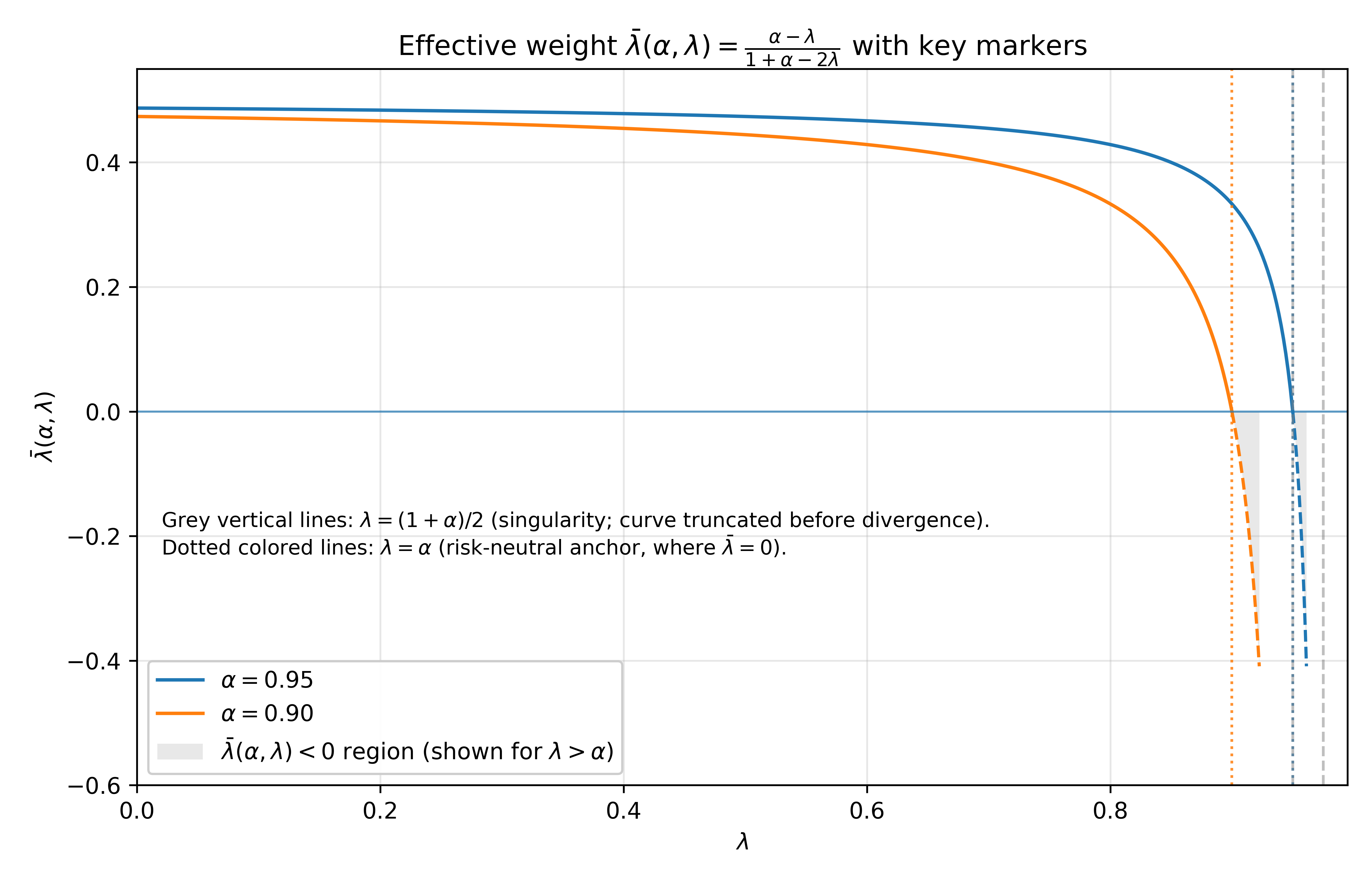
Figure 2 shows that $\bar{\lambda}(\alpha,\lambda)$ decreases to $0$ as $\lambda$ approaches $\alpha$, clarifying the risk-neutral anchor at $\lambda=\alpha$. The mapping diverges at $\lambda=(1+\alpha)/2$ and becomes negative for $\lambda>\alpha$, motivating $\lambda\leq\alpha$. Practically, the curves are relatively flat over moderate $\lambda$ (e.g., $\lambda\in[0,0.8]$), so many values in this range induce similar effective tail weights.

To determine whether the certainty-equivalent cost $\Phi_{\alpha,\lambda}(Y)$ falls in the buffer (yellow) region or the mean-excess (red) region shown in Figure 1, we define

$$\tau_{\alpha}(Y):=\frac{\mathrm{VaR}_{\alpha}(Y)-\mathbb{E}[Y]}{\mathrm{CVaR}_{\alpha}(Y)-\mathbb{E}[Y]}.$$ (17)

$\Phi_{\alpha,\lambda}(Y)$ lies in the buffer interval (Mean–$\mathrm{VaR}_{\alpha}$) iff $\bar{\lambda}(\alpha,\lambda)\leq\tau_{\alpha}(Y)$, and it lies in the mean-excess segment ($\mathrm{VaR}_{\alpha}$–$\mathrm{CVaR}_{\alpha}$) only if $\bar{\lambda}(\alpha,\lambda)\geq\tau_{\alpha}(Y)$. Under (14) with $\lambda\leq\alpha$, $\bar{\lambda}$ is capped by $\alpha/(1+\alpha)<1/2$, so mean-excess positioning requires $\tau_{\alpha}(Y)\leq\alpha/(1+\alpha)$; otherwise, $\Phi_{\alpha,\lambda}(Y)$ remains in the buffer region for all admissible $\lambda$.

Embedding tail-sensitive costs in an exponential logit kernel can amplify risk in equilibrium. In the RU form, $\mathrm{CVaR}_{\alpha}$ scales tail exceedance by $1/(1-\alpha)$. In our potential-based models, the tail term effectively enters with multiplier $\mathcal{O}\!\left(\lambda/(1-\alpha)\right)$. For high reliability levels (e.g., $\alpha=0.95$ where $1/(1-\alpha)=20$), the combination with $\exp(-\theta\cdot)$ can induce probability collapse, extreme sensitivity, and numerical instability. We therefore impose $\lambda\leq\alpha/(1+\alpha)$, which bounds tail amplification as $\frac{\lambda}{1-\alpha}\ \leq\ \frac{\alpha}{1-\alpha^{2}}$. For $\alpha=0.95$, this reduces the maximum factor from $20$ to approximately $9.74$, tempering tail sensitivity with no rescaling to the travel time units.

We use two complementary risk-sensitive truncated-logit TSUE constructs. Approach A (path-based) applies the certainty equivalent $\Phi_{\alpha,\lambda}$ directly to each path travel time in the kernel. This captures tail-aware perception and makes truncation driven by reliability. However, it breaks link-additive separability and makes the active tail set flow-dependent. A convex form exists only in special cases. Approaches B1–B2 (potential-based) apply the same risk functional at the system level: B1 to a scenario-dependent TSUE potential, B2 to the congestion potential only. Both recover risk-adjusted generalized costs from the Karush-Kuhn-Tucker (KKT) conditions. For $\lambda\leq\alpha$, this yields a single convex stochastic program and preserves standard TSUE computational structure. B2 keeps $\theta$ outside $\Phi_{\alpha,\lambda}$, retaining its interpretation as the logit dispersion parameter.

4.2 Approach A: Path-based risk perception embedded in TSUE

Approach A replaces the deterministic cost in truncated logit by a risk-adjusted certainty equivalent of random path travel time. Under scenarios $\{\xi^{1},\ldots,\xi^{S}\}$ with probabilities $p_{s}$, let $t_{a}^{s}(x_{a})$ be scenario $s$ link travel time, and define the path travel time $t_{k}^{od,s}(v):=\sum_{a\in k}t_{a}^{s}(x_{a}),\quad s=1,\ldots,S$, with link flows $x_{a}=\sum_{o,d}\sum_{k\in K_{od}}f_{k}^{od}\delta_{a,k}^{od}$. For each $k\in K_{od}$, the deterministic generalized cost entering truncated logit is the normalized certainty equivalent

$$\phi_{k,\alpha,\lambda}^{od}(v):=\Phi_{\alpha,\lambda}\!\left(t_{k}^{od}(v,\xi)\right)=\bigl(1-\bar{\lambda}(\alpha,\lambda)\bigr)\,\sum_{s=1}^{S}p_{s}\,t_{k}^{od,s}(v)+\bar{\lambda}(\alpha,\lambda)\,\mathrm{CVaR}_{\alpha}\!\left(t_{k}^{od}(v,\xi)\right),\qquad\lambda\leq\alpha,$$ (18)

anchored at $\lambda=\alpha$ where $\phi_{k,\alpha,\alpha}^{od}(v)=\sum_{s=1}^{S}p_{s}\,t_{k}^{od,s}(v)$ (risk-neutral).

Using the RU representation, $c_{k}^{od}(v)$ admits

$$\mathrm{CVaR}_{\alpha}\!\left(t_{k}^{od}(v,\xi)\right)=\min_{\gamma_{k}^{od}\in\mathbb{R}}\left\{\gamma_{k}^{od}+\frac{1}{1-\alpha}\sum_{s=1}^{S}p_{s}\,u_{k,s}^{od}\ \middle|\ u_{k,s}^{od}\geq t_{k}^{od,s}(v)-\gamma_{k}^{od},\ \ u_{k,s}^{od}\geq 0\right\}.$$ (19)

Given $\phi_{k,\alpha,\lambda}^{od}(v)$, the admissible set is $K_{od}^{\alpha,\lambda}(v):=\left\{k\in K_{od}\ \middle|\ \phi_{k,\alpha,\lambda}^{od}(v)<\pi_{od}\right\}$, and truncated-logit choice probabilities are

$$P_{k}^{od}(v)=\frac{\left[\exp\!\left(-\theta\left(\phi_{k,\alpha,\lambda}^{od}(v)-\pi_{od}\right)\right)-1\right]_{+}}{\sum_{\ell\in K_{od}}\left[\exp\!\left(-\theta\left(\phi_{\ell,\alpha,\lambda}^{od}(v)-\pi_{od}\right)\right)-1\right]_{+}},\qquad k\in K_{od}.$$ (20)

The corresponding risk-averse truncated-logit equilibrium is the fixed point

$$f_{k}^{od}=q_{od}\,P_{k}^{od}(v),\qquad x_{a}=\sum_{o,d}\sum_{k\in K_{od}}f_{k}^{od}\delta_{a,k}^{od},\qquad f_{k}^{od}\geq 0.$$ (21)

Approach A needs a natural fixed-point/variational inequality formulation. Applying a tail functional (CVaR/mean–CVaR) to path sums breaks link-additive separability, introduces cross-path coupling on overlapping routes, and makes the active tail set flow-dependent. Together with the endogenous truncation set $K_{od}^{\alpha,\lambda}(v)$, these features typically preclude a global Beckmann-type potential except in special cases (e.g., separable risk across links or non-overlapping paths). Hence, Approach A is best tackled by fixed-point method (e.g, method of successive averages).

4.3 Approach B1: TSUE via a certainty equivalent of the total TSUE potential

Approach B1 applies the risk functional to the full scenario-dependent TSUE potential, i.e., to congestion plus the entropy regularization. It admits a single-level convex stochastic programming reformulation for $\lambda\leq\alpha$.

Let $\Psi(f)$ denote the standard entropy regularization term used in TSUE:

$$\Psi(f):=\sum_{o,d}\sum_{k\in K_{od}}\Big[(f_{k}^{od}+1)\ln(f_{k}^{od}+1)-f_{k}^{od}\Big].$$ (22)

Define the scenario-dependent congestion potential as $\widehat{Z}^{s}(f):=\sum_{a\in A}\int_{0}^{x_{a}}t_{a}^{s}(\omega)\,d\omega,\quad x_{a}=\sum_{o,d}\sum_{k\in K_{od}}f_{k}^{od}\delta_{a,k}^{od},\quad s=1,\ldots,S,$ and the corresponding total scenario TSUE potential as

$$Z^{s}(f):=\widehat{Z}^{s}(f)+\frac{1}{\theta}\Psi(f),\qquad s=1,\ldots,S.$$ (23)

Let $Z(f,\xi)$ denote the random variable taking values $Z^{s}(f)$ with probability $p_{s}$. Under Approach B1, the system objective is the certainty equivalent of $Z(f,\xi)$:

$$\Phi_{\alpha,\lambda}^{\mathrm{B1}}(f):=\Phi_{\alpha,\lambda}\!\big(Z(f,\xi)\big)=\bigl(1-\bar{\lambda}(\alpha,\lambda)\bigr)\,\mathbb{E}\!\left[Z(f,\xi)\right]+\bar{\lambda}(\alpha,\lambda)\,\mathrm{CVaR}_{\alpha}\!\left(Z(f,\xi)\right),\qquad\lambda\leq\alpha.$$ (24)

The risk-averse TSUE under Approach B1 is minimize the $\Phi_{\alpha,\lambda}^{\mathrm{B1}}(f)$. Using the RU representation of $\mathrm{CVaR}_{\alpha}(\cdot)$, the problem is equivalent to:

$$\min_{f,\gamma,\;u_{s}\geq 0}\ \bigl(1-\bar{\lambda}(\alpha,\lambda)\bigr)\sum_{s=1}^{S}p_{s}\,Z^{s}(f)+\bar{\lambda}(\alpha,\lambda)\,\gamma+\frac{\bar{\lambda}(\alpha,\lambda)}{1-\alpha}\sum_{s=1}^{S}p_{s}\,u_{s}$$ (25a)

s.t. $$u_{s}\ \geq\ Z^{s}(f)-\gamma,\quad u_{s}\ \geq\ 0,\quad\eqref{eq:demand_conservation}--\eqref{eq:nennegative},\quad s=1,\ldots,S,\quad\gamma\in\mathbb{R}$$ (25b)

Convexity follows because each $Z^{s}(f)$ is convex in $f$ (Beckmann potential plus convex entropy term), and the RU epigraph form preserves convexity.

4.4 Approach B2: TSUE via a certainty equivalent of the congestion potential

Approach B2 applies the risk functional to the scenario-dependent congestion potential only, and keeps the entropy term outside the risk functional. This preserves the behavioral interpretation of $\theta$ as the (inverse) dispersion parameter of the truncated-logit kernel.

Let $\widehat{Z}(f,\xi)$ denote the random variable taking values $\widehat{Z}^{s}(f)$ with probability $p_{s}$. Under Approach B2, the risk-adjusted system objective is

$$\Phi_{\alpha,\lambda}^{\mathrm{B2}}(f):=\Phi_{\alpha,\lambda}\!\big(\widehat{Z}(f,\xi)\big)=\bigl(1-\bar{\lambda}(\alpha,\lambda)\bigr)\,\mathbb{E}\!\left[\widehat{Z}(f,\xi)\right]+\bar{\lambda}(\alpha,\lambda)\,\mathrm{CVaR}_{\alpha}\!\left(\widehat{Z}(f,\xi)\right),\qquad\lambda\leq\alpha.$$ (26)

The risk-averse TSUE is formulated as

$$\min_{f}\ \Phi_{\alpha,\lambda}^{\mathrm{B2}}(f)+\frac{1}{\theta}\Psi(f)\quad\text{s.t.}\quad\eqref{eq:demand_conservation}--\eqref{eq:nennegative}.$$ (27)

Let $\widehat{Z}^{s}(f):=\widehat{Z}(f,\xi^{s})$. Then,

$$\mathrm{CVaR}_{\alpha}(\widehat{Z}(f,\xi))=\min_{\gamma\in\mathbb{R},\ u_{s}\geq 0}\left\{\gamma+\frac{1}{1-\alpha}\sum_{s=1}^{S}p_{s}u_{s}\ \middle|\ u_{s}\geq\widehat{Z}^{s}(f)-\gamma,\ \ s=1,\ldots,S\right\}.$$ (28)

At optimality of (28), the KKT conditions imply the existence of tail weights $\chi_{s}\in[0,1]$ such that $0\leq\chi_{s}\leq 1,\sum_{s=1}^{S}p_{s}\chi_{s}=1-\alpha,$ and a subgradient of $\mathrm{CVaR}_{\alpha}(\widehat{Z}(f,\xi))$ can be written as a tail-weighted combination of scenario gradients:

$$\partial_{f}\,\mathrm{CVaR}_{\alpha}(\widehat{Z}(f,\xi))=\frac{1}{1-\alpha}\sum_{s=1}^{S}p_{s}\chi_{s}\nabla_{f}\widehat{Z}^{s}(f).$$ (29)

Intuitively, $\chi_{s}=1$ for scenarios strictly in the worst $(1-\alpha)$ tail, $\chi_{s}=0$ for non-tail scenarios, and $\chi_{s}\in(0,1)$ only for scenarios on the VaR boundary.

Define the scenario $s$ marginal path travel time induced by the Beckmann potential:

$$\tau_{k}^{od,s}(v):=\frac{\partial\widehat{Z}^{s}(f)}{\partial f_{k}^{od}}=\sum_{a\in k}t_{a}^{s}(x_{a}),\qquad k\in K_{od},\ s=1,\ldots,S.$$ (30)

Combining (26) with (29)–(30) yields the induced risk-adjusted generalized marginal cost

$$g_{k}^{od}(f):=\partial_{f_{k}^{od}}\Phi_{\alpha,\lambda}^{\mathrm{B2}}(f)=\bigl(1-\bar{\lambda}(\alpha,\lambda)\bigr)\sum_{s=1}^{S}p_{s}\,\tau_{k}^{od,s}(v)+\frac{\bar{\lambda}(\alpha,\lambda)}{1-\alpha}\sum_{s=1}^{S}p_{s}\,\chi_{s}\,\tau_{k}^{od,s}(v).$$ (31)

Thus, under Approach B2, the deterministic cost that governs truncated logit screening and weighting is the endogenously induced generalized marginal cost $g_{k}^{od}(f)$.

Let $\mu_{od}$ be the Lagrange multiplier associated with the OD conservation constraint $\sum_{k\in K_{od}}f_{k}^{od}=q_{od}$. The KKT conditions for (27) imply that, for each OD pair and each path $k\in K_{od}$,

$$g_{k}^{od}(f)+\frac{1}{\theta}\ln\!\left(f_{k}^{od}+1\right)=\mu_{od}\quad\text{if }f_{k}^{od}>0,$$ (32)

and $g_{k}^{od}(f)\geq\mu_{od}$ if $f_{k}^{od}=0$. Solving (32) and enforcing nonnegativity yields the truncated form

$$f_{k}^{od}=\Big[\exp\!\big(\theta(\mu_{od}-g_{k}^{od}(f))\big)-1\Big]_{+}.$$ (33)

Therefore, the induced choice probabilities $P_{k}^{od}=f_{k}^{od}/q_{od}$ admit a truncated-logit kernel with deterministic cost $g_{k}^{od}(f)$:

$$P_{k}^{od}(f)=\frac{\Big[\exp\!\big(-\theta(g_{k}^{od}(f)-\mu_{od})\big)-1\Big]_{+}}{\sum_{\ell\in K_{od}}\Big[\exp\!\big(-\theta(g_{\ell}^{od}(f)-\mu_{od})\big)-1\Big]_{+}}.$$ (34)

In applications where a feasibility threshold $\pi_{od}$ is specified (e.g., a travel-time budget), $\mu_{od}$ can be interpreted as the endogenous reservation cost consistent with demand $q_{od}$, or $\pi_{od}$ may be calibrated to match $\mu_{od}$ at equilibrium.

Using (28), (27) is equivalent to the following single-level convex program:

$$\min_{f,\gamma,\;u_{s}\geq 0}\ \bigl(1-\bar{\lambda}(\alpha,\lambda)\bigr)\sum_{s=1}^{S}p_{s}\widehat{Z}^{s}(f)+\bar{\lambda}(\alpha,\lambda)\,\gamma+\frac{\bar{\lambda}(\alpha,\lambda)}{1-\alpha}\sum_{s=1}^{S}p_{s}u_{s}+\frac{1}{\theta}\Psi(f)$$ (35a)

s.t. $$u_{s}\ \geq\ \widehat{Z}^{s}(f)-\gamma,\quad u_{s}\ \geq\ 0,\quad\eqref{eq:demand_conservation}--\eqref{eq:nennegative},\quad s=1,\ldots,S,\quad\gamma\in\mathbb{R}$$ (35b)

Proposition 4.5

Suppose that, for every link $a\in A$ and every scenario $s=1,\ldots,S$, the scenario-dependent link travel-time function $t_{a}^{s}(x_{a})$ is continuous and nondecreasing in $x_{a}\geq 0$. Let $\theta>0$, $\alpha\in(0,1)$, and $0\leq\lambda\leq\alpha$, so that the effective mixing weight defined in (14) satisfies $\bar{\lambda}(\alpha,\lambda)\in[0,1]$. Then Approaches B1 and B2 have the same unique optimal path-flow solution.

Proof 4.6

Proof. The proof can be found in Appendix I.

Proposition 4.7

The mathematical program in (25a) and  (35a) can be solved as a regular TSUE/SUE problem with auxiliary variables for the CVaR representation.

Proof 4.8

Proof. The proof can be found in Appendix J.

4.5 Path- and potential-based risk equivalence under regime dominance

Approach A applies the certainty equivalent in (15) directly to path travel times, yielding the path-based generalized cost in (18). Approach B2 applies the same risk functional to the scenario-dependent congestion potential, and its induced generalized marginal cost is given by (31). These two constructions generally do not coincide because the CVaR tail selected by a path travel-time random variable need not be the same as the CVaR tail selected by the congestion potential. This subsection identifies conditions under which the two costs coincide.

Assume that the scenario-dependent link travel times admit a common network-wide ordering from mild to severe:

$$t_{a}^{1}(x)\leq t_{a}^{2}(x)\leq\cdots\leq t_{a}^{S}(x),\qquad\forall a\in A,\ \forall x\geq 0.$$ (36)

This condition captures regime-level hazards, such as $\mathrm{NR}\prec\mathrm{HR}\prec\mathrm{FL}$, that worsen all links in the same scenario order, although the magnitude of deterioration may differ across links.

Proposition 4.9 (Equivalence under network-wide regime dominance)

Consider any feasible path-flow vector $f$ and its induced link-flow vector $v$. Under the parameter domain used in (14), if (36) holds and the CVaR subgradient selector is chosen consistently at VaR ties, then for every OD pair $(o,d)$ and every path $k\in K_{od}$,

$$\phi_{k,\alpha,\lambda}^{od}(v)=g_{k}^{od}(f).$$ (37)

Consequently, if the admissibility baselines are aligned, for example $\pi_{od}=\mu_{od}$ at equilibrium, then the truncated-logit kernels in (20) and (34) induce the same admissible path sets, the same choice probabilities, and hence the same equilibrium path and link flows.

Proof 4.10

Proof. Condition (36) implies that every path travel-time random variable appearing in (18) inherits the same scenario ordering. Since the scenario congestion potential is obtained by integrating the same ordered link travel-time functions, the random congestion potential in (26) also inherits the same scenario ordering.

Therefore, the path-level CVaR terms in (18) and the potential-level CVaR term whose subgradient is represented in (29) use the same tail-weight selector. By (30), the scenario gradient of the congestion potential with respect to path flow is the corresponding scenario path travel time. Substituting the common tail selector into (31) therefore gives the same weighted scenario combination as the path-based cost in (18). Hence (37) follows.

If $\pi_{od}=\mu_{od}$, then (20) and (34) have the same deterministic cost and the same reservation baseline for each OD pair. The admissible sets and normalized probability weights are therefore identical.

Remark 4.11 (Fixed-$\alpha$ common-tail equivalence)

The regime dominance condition in (36) is sufficient but not necessary. For a fixed $\alpha$, the equivalence only requires a common CVaR tail selector.

Let $\chi_{k,s}^{A,od}(f)$ denote a valid CVaR tail selector for the path-level CVaR term in (18), and let $\chi_{s}^{B2}(f)$ denote the selector appearing in the B2 subgradient representation (29). If, for every feasible $f$,

$$\chi_{k,s}^{A,od}(f)=\chi_{s}^{B2}(f),\qquad\forall(o,d),\ \forall k\in K_{od},\ \forall s=1,\ldots,S,$$ (38)

then the same argument as in Proposition 4.9 gives $\phi_{k,\alpha,\lambda}^{od}(v)=g_{k}^{od}(f)$ for all OD pairs and paths.

Thus, a complete global ranking of all scenarios is not required at a fixed $\alpha$. Internal orderings inside the non-tail block and inside the tail block may differ across paths, provided that the induced CVaR tail selector in (38) is common.

Corollary 4.12 (Choosing $\alpha$ at a regime boundary)

Suppose the scenario set can be partitioned into a non-tail block and a severe regime block,

$$\Xi=L_{\alpha}\cup H_{\alpha},$$

such that

$$t_{a}^{\ell}(x)\leq t_{a}^{h}(x),\qquad\forall a\in A,\ \forall x\geq 0,\ \forall\ell\in L_{\alpha},\ \forall h\in H_{\alpha},$$ (39)

while the ordering within $L_{\alpha}$ and within $H_{\alpha}$ may be arbitrary. If

$$\sum_{h\in H_{\alpha}}p_{h}=1-\alpha,$$ (40)

then (38) holds. Hence Approaches A and B2 induce the same generalized path costs.

Proof 4.13

Proof. By (39), every scenario in $H_{\alpha}$ is at least as severe as every scenario in $L_{\alpha}$ for every link; therefore, it is also true for every path and for the congestion potential. By (40), the severe block has exactly the CVaR tail probability mass. Hence the same tail selector assigns full weight to scenarios in $H_{\alpha}$ and zero weight to scenarios in $L_{\alpha}$ for all path travel-time random variables and for the congestion potential. The condition in (38) follows, and the result follows from Remark 4.11.

Corollary 4.12 gives an operational interpretation of $\alpha$. If a set of regimes is severe for the network as a whole, then $\alpha$ can be chosen at the boundary between ordinary and severe regimes, so that $1-\alpha$ equals the probability mass of the severe block. For example, if two paths rank scenarios as

$$a,b,c\mid d,e,f\qquad\text{and}\qquad b,c,a\mid e,f,d,$$

where the vertical bar denotes the $\alpha$ cutoff, then the internal orderings within $\{a,b,c\}$ and within $\{d,e,f\}$ do not matter. The expectation term is order-free, and the CVaR term uses the same tail block $\{d,e,f\}$. In contrast, if $\alpha$ cuts inside a heterogeneous severe block, different paths may select different VaR-boundary or tail scenarios, so (38) may fail and the equivalence between Approaches A and B2 is no longer guaranteed.

Finally, when $\lambda=\alpha$, (14) gives the risk-neutral case. The CVaR selector no longer affects the generalized costs, so the common-tail conditions above are unnecessary.

5 $1$-Wasserstein distributionally robust optimization (TSUE-DRO)

The certainty equivalent $\Phi_{\alpha,\lambda}$ in (15) encodes behavioral risk sensitivity conditional on a prescribed probability law for $\xi$. In Approaches A and B1–B2, this law enters through the scenario probabilities used to compute $\mathbb{E}[\cdot]$ and $\mathrm{CVaR}_{\alpha}(\cdot)$. In hazard-prone networks, however, the law of $\xi$ is typically unknown and must be learned from limited, regime-mixed, and nonstationary data. Instability is often driven by distributional misspecification rather than by $(\alpha,\lambda)$.

This is especially evident under the normalized coupling (14). The risk premium in (16) scales with $\mathrm{CVaR}_{\alpha}(Y)-\mathbb{E}[Y]$, a tail-driven quantity that is difficult to estimate reliably and can shift under regime changes. Truncated-logit screening introduces threshold nonlinearity. When perceived route costs lie near feasibility cutoffs, small probability errors can flip admissibility and change the active choice set discontinuously. Thus, even if $\bar{\lambda}(\alpha,\lambda)$ varies smoothly, the induced equilibrium may still be fragile when applied to new observations not included in the dataset used to estimate the scenario probabilities (i.e., out-of-sample). To hedge this epistemic uncertainty, we replace the nominal law with an ambiguity set $\mathcal{D}$ and optimize the same normalized mean–CVaR objective against the worst $Q\in\mathcal{D}$. The Wasserstein radius $\rho$ controls distributional robustness, while $(\alpha,\lambda)$ control risk preference conditional on a given law. Wasserstein-ball DRO around an empirical measure produces finite-sample guarantees and strong dual reformulations (Gao 2023).

5.1 Robust mean-CVaR certainty equivalent over a Wasserstein ball

Let $Z(f,\xi)$ denote the (scenario-dependent) TSUE system potential under uncertainty $\xi$. We reformulate the normalized mean-CVaR certainty equivalent (Section 4) as a robust optimization (RO) formulation over an ambiguity set $\mathcal{D}$:

$$\Phi_{\alpha,\lambda}^{\mathrm{DRO}}(f)=\sup_{Q\in\mathcal{D}}\left\{\bigl(1-\bar{\lambda}(\alpha,\lambda)\bigr)\,\mathbb{E}_{Q}[Z(f,\xi)]+\bar{\lambda}(\alpha,\lambda)\,\operatorname{CVaR}_{\alpha,Q}[Z(f,\xi)]\right\},\quad 0\leq\lambda\leq\alpha<1,$$ (41)

Let $P_{0}$ be the nominal (empirical) distribution of $\xi$. The $1$-Wasserstein distance is $W_{1}\left(Q,P_{0}\right)=\inf_{\pi\in\Pi\left(Q,P_{0}\right)}\mathbb{E}_{\left(\xi,\xi_{0}\right)\sim\pi}\left[d\left(\xi,\xi_{0}\right)\right],$ where $\Pi(Q,P_{0})$ is the set of couplings and $d(\cdot,\cdot)$ is a ground metric. We adopt the Euclidean metric $d\left(\xi,\xi_{0}\right)=\left\|\xi-\xi_{0}\right\|_{2}$, which is standard in continuous transportation settings and yields sharp statistical rates (Panaretos and Zemel 2019). For $\rho>0$, define the $1$-Wasserstein ambiguity set $\mathcal{D}=\left\{Q\mid W_{1}\left(Q,P_{0}\right)\leq\rho\right\},\rho>0$. The TSUE-DRO problem is

$$\min_{f}\ \Phi_{\alpha,\lambda}^{\mathrm{DRO}}(f)\quad\text{s.t. }\eqref{eq:demand_conservation}-\eqref{eq:nennegative}.$$ (42)

The radius $\rho$ has physical units measured in the same units as $\xi$ under the chosen ground metric. It can be interpreted as an average perturbation of inputs (e.g., under extreme weather $+1$ inch rainfall, $-10\%$ road capacity). Unlike $f$-divergence ambiguity sets, Wasserstein balls can shift probability mass to nearby but unobserved scenarios. This addresses support mismatch and enables a controlled stress test of adverse realizations. The ambiguity set itself does not require light-tailedness. However, the finite-sample radius selection rule in Section 5.3 assumes a light-tailed or compact-support $\widehat{P}$. When heavy tails are expected, $\rho$ can be selected via out-of-sample validation, robust resampling, or alternative concentration bounds tailored to heavy-tailed distributions.

5.2 Connection to risk-averse TSUE (Approach B) and B1-DRO vs. B2-DRO

We extend the potential-based risk-averse TSUE formulation (Approach B in Section 4) to distributional ambiguity. Recall that the scenario-dependent TSUE potential can be written as $Z(f,\xi)=\widehat{Z}(f,\xi)+\frac{1}{\theta}\Psi(f)$, where $\widehat{Z}(f,\xi)$ is the congestion potential (scenario-dependent) and $\Psi(f)$ is the entropy regularization (scenario-invariant). This gives rise to two natural DRO specifications. B1–DRO incorporates robustness in the random variable $Z(f,\xi)$ inside the risk functional. B2-DRO adds robustness to $\widehat{Z}(f,\xi)$ and keep the scenario-invariant entropy term $\tfrac{1}{\theta}\Psi(f)$ outside the risk functional.

Proposition 5.1

Fix $\alpha\in(0,1)$ and $\lambda\leq\alpha$, and let $\bar{\lambda}=\bar{\lambda}(\alpha,\lambda)$. Let $Y(\xi)$ be any integrable random cost and let $b\in\mathbb{R}$ be a constant (i.e., $b$ does not depend on $\xi$). Then, for any ambiguity set $\mathcal{D}$,

$$\sup_{Q\in\mathcal{D}}\left\{(1-\bar{\lambda})\,\mathbb{E}_{Q}[Y+b]+\bar{\lambda}\,\operatorname{CVaR}_{\alpha,Q}(Y+b)\right\}=\sup_{Q\in\mathcal{D}}\left\{(1-\bar{\lambda})\,\mathbb{E}_{Q}[Y]+\bar{\lambda}\,\operatorname{CVaR}_{\alpha,Q}(Y)\right\}+b.$$ (43)

Consequently, with $c(f):=\tfrac{1}{\theta}\Psi(f)$ and $Y(\xi)=\widehat{Z}(f,\xi)$, we have for every feasible $f$,

$$\sup_{Q\in\mathcal{D}}\left\{(1-\bar{\lambda})\,\mathbb{E}_{Q}[Z(f,\xi)]+\bar{\lambda}\,\operatorname{CVaR}_{\alpha,Q}(Z(f,\xi))\right\}=\sup_{Q\in\mathcal{D}}\left\{(1-\bar{\lambda})\,\mathbb{E}_{Q}[\widehat{Z}(f,\xi)]+\bar{\lambda}\,\operatorname{CVaR}_{\alpha,Q}(\widehat{Z}(f,\xi))\right\}+\frac{1}{\theta}\Psi(f),$$ (44)

hence, B1–DRO and B2–DRO define identical optimization problems and admit the same optimal solutions.

Proof 5.2

Proof. The proof can be found in Appendix K.

The identity above uses that $b$ is constant with respect to $\xi$ (for fixed $f$). In general, $\operatorname{CVaR}_{\alpha}(Y+U)\neq\operatorname{CVaR}_{\alpha}(Y)+\operatorname{CVaR}_{\alpha}(U)$ when $U$ is random. Here, $\Psi(f)/\theta$ is scenario-invariant and therefore constitutes a constant shift in $\xi$. Accordingly, we present the DRO development for a generic $Z(f,\xi)$. When emphasizing the behavioral interpretation of $\theta$ as the dispersion parameter of the truncated-logit kernel, we prefer the B2-DRO viewpoint (only robust congestion and keep $\Psi(f)/\theta$ outside the risk functional), noting that it is exactly equivalent to B1-DRO under the normalized $(\alpha,\lambda)$-coupled certainty equivalent. When emphasizing the behavioral interpretation of $\theta$ as the dispersion parameter of the truncated-logit kernel, we present results using the B2-DRO form.

5.3 Finite-sample guarantee

Suppose we draw $N$ independent samples $\xi^{1},\ldots,\xi^{N}$ from the unknown true distribution $\widehat{P}$. The empirical distribution is $P_{0}=\frac{1}{N}\sum_{i=1}^{N}\delta_{\xi^{i}}.$

The random vectors $\xi^{1},\ldots,\xi^{N}\in\mathbb{R}^{m}$ are independent and identically distributed according to an unknown distribution $\widehat{P}$. Moreover, $\widehat{P}$ is light-tailed: there exists an exponent $\nu>1$ such that $A\;:=\;\mathbb{E}_{\widehat{P}}\!\Big[\exp\!\big(\|\xi\|_{2}^{\nu}\big)\Big]\;<\;\infty$. As a special case, this assumption holds trivially if the support $\Xi$ of $\xi$ is compact.

Proposition 5.3 (Measure concentration, Theorem 3.4 in Mohajerin Esfahani and Kuhn (2018))

If Assumption 5.3 holds, then for every $N\geq 1$, $\rho>0$, and $m\neq 2$,

$$\text{Pr}^{N}\!\left\{W_{1}\!\bigl(\widehat{P},P_{0}\bigr)\,\geq\,\rho\right\}\;\leq\;\begin{cases}c_{1}\exp\!\bigl(-c_{2}N\,\rho^{\max\{m,2\}}\bigr),&0<\rho\leq 1,\\[4.0pt] c_{1}\exp\!\bigl(-c_{2}N\,\rho^{\nu}\bigr),&\rho>1,\end{cases}$$ (45)

where $c_{1},c_{2}>0$ depend only on $(m,\nu,A)$. (A similar but slightly more complicated inequality also holds for the special case $m=2$; see Mohajerin Esfahani and Kuhn (2018).)

Proposition 5.3 allows us to choose a radius that contains $\widehat{P}$ with confidence $1-\delta$. Equating the right-hand side of (45) to $\delta$ and solving for $\rho$ yields the calibration

$$\rho_{N,\delta}:=\rho_{N}(\delta)=\begin{cases}\left(\dfrac{\log(c_{1}\delta^{-1})}{c_{2}N}\right)^{1/\max\{m,2\}},&N\;\geq\;\dfrac{\log(c_{1}\delta^{-1})}{c_{2}},\\[12.0pt] \left(\dfrac{\log(c_{1}\delta^{-1})}{c_{2}N}\right)^{1/\nu},&N\;<\;\dfrac{\log(c_{1}\delta^{-1})}{c_{2}}.\end{cases}$$ (46)

Hence, with probability at least $1-\delta$, $W_{1}\!\bigl(\widehat{P},P_{0}\bigr)\leq\rho_{N,\delta},$ so the Wasserstein ball of radius $\rho_{N,\delta}$ around $P_{0}$ is a $(1-\delta)$-confidence set for $\widehat{P}$. One may set $\rho=\rho_{N,\delta}$ for a desired confidence level, tune $\rho$ via out-of-sample validation, or select it based on policy tolerances (e.g., robustness to $\pm 1$ inch average rainfall). The Wasserstein radius trades off robustness and conservatism.

5.4 Dual reformulation via CVaR epigraph and Wasserstein duality

Let $P_{0}=\frac{1}{N}\sum_{i=1}^{N}\delta_{\xi^{i}}$ be the empirical distribution and $\mathcal{D}:=\{Q:W_{1}(Q,P_{0})\leq\rho\}$ the $1$-Wasserstein ambiguity set (with ground metric $\|\cdot\|_{2}$). For fixed $f$ and $(\alpha,\lambda)$ with $\lambda\leq\alpha$, define the hinge-augmented payoff

$$g_{t}(f,\xi):=\bigl(1-\bar{\lambda}(\alpha,\lambda)\bigr)\,Z(f,\xi)+\frac{\bar{\lambda}(\alpha,\lambda)}{1-\alpha}\,\bigl(Z(f,\xi)-t\bigr)_{+},\qquad t\in\mathbb{R},$$ (47)

where $\bar{\lambda}(\alpha,\lambda)$ is given in (14).

Let $(\Xi,\|\cdot\|_{2})$ be a closed subset of $\mathbb{R}^{m}$. For every feasible $f$ and every $t\in\mathbb{R}$, the map $\xi\mapsto Z(f,\xi)$ is measurable, upper semicontinuous, and has at most linear growth on $\Xi$, ensuring that all expectations under distributions in $\mathcal{D}$ are well-defined.

Proposition 5.4

Under Assumption 5.4, for all feasible $f$,

$$\Phi_{\alpha,\lambda}^{\mathrm{DRO}}(f)\;\leq\;\inf_{\begin{subarray}{c}t\in\mathbb{R}\\ \kappa\geq 0\end{subarray}}\left\{\bar{\lambda}(\alpha,\lambda)\,t+\kappa\rho+\frac{1}{N}\sum_{i=1}^{N}\sup_{\xi\in\Xi}\Big(g_{t}(f,\xi)-\kappa\|\xi-\xi^{i}\|_{2}\Big)\right\}.$$ (48)

Moreover, if the minimax interchange $\sup_{Q\in\mathcal{D}}\inf_{t}=\inf_{t}\sup_{Q\in\mathcal{D}}$ holds for the epigraph form, and $\xi\mapsto g_{t}(f,\xi)$ satisfies the piecewise-concave condition of (Mohajerin Esfahani and Kuhn 2018, Assumption 4.1) (e.g., $g_{t}(f,\cdot)$ is piecewise affine on a convex closed $\Xi$), then the inequality in (48) is tight and becomes an equality. In that case, introducing epigraph variables $s_{i}\in\mathbb{R}$ yields the exact semi-infinite convex reformulation

$$\min_{f,t,\kappa,\{s_{i}\}}~~ \bar{\lambda}(\alpha,\lambda)\,t+\kappa\rho+\frac{1}{N}\sum_{i=1}^{N}s_{i}$$ (49a)

s.t. $$s_{i}\ \geq\ g_{t}(f,\xi)-\kappa\|\xi-\xi^{i}\|_{2},\quad\kappa\geq 0,\quad\text{\eqref{eq:demand_conservation}--\eqref{eq:nennegative}},\quad t\in\mathbb{R},\quad\forall\xi\in\Xi,\ \ i=1,\ldots,N,$$ (49b)

Proof 5.5

Proof. The proof can be found in Appendix L.

5.5 Tractable reformulations

The tractability of (49) depends on the ability to solve or represent the inner maximizations over $\Xi$. We outline two standard cases.

5.5.1 Case 1: Discrete/finite support $\Xi$

If the support is restricted to a finite scenario set $\Xi=\{\zeta^{1},\ldots,\zeta^{M}\}$ (e.g., a discretized hazard library), then the semi-infinite constraints in (49) reduce to finitely many linear (in $s_{i}$) constraints: $s_{i}\ \geq\ g_{t}(f,\zeta^{j})-\kappa\|\zeta^{j}-\xi^{i}\|_{2},\quad\forall i=1,\ldots,N,\ \forall j=1,\ldots,M.$ The resulting program is a finite-dimensional convex optimization problem that can be solved by standard solvers; its size scales with $NM$.

5.5.2 Case 2: Affine dependence on $\xi$ and exact second-order conic programming reduction

A closed-form conic reduction is available when $Z(f,\xi)$ is affine in $\xi$ (or when it is approximated by a convex piecewise-affine surrogate in $\xi$).

Assume that for each feasible $f$, $Z(f,\xi)$ is affine in $\xi$ on $\Xi=\mathbb{R}^{m}$: $Z(f,\xi)=Z_{0}(f)+h(f)^{\top}\xi,$ where $Z_{0}(f)\in\mathbb{R}$ and $h(f)\in\mathbb{R}^{m}$. Moreover, $h(f)$ is affine in $f$ so that the constraints $\|h(f)\|_{2}\leq\cdot$ are second-order conic programming (SOCP) representable.

Under Assumption 5.5.2, $g_{t}(f,\xi)$ in (47) is the maximum of two affine functions in $\xi$:

$$g_{t}(f,\xi)=\max\{a_{0}(f)^{\top}\xi+b_{0}(f),\ a_{1}(f)^{\top}\xi+b_{1}(f,t)\},$$ (50)

with $a_{0}(f)=(1-\bar{\lambda})\,h(f),\quad b_{0}(f)=(1-\bar{\lambda})\,Z_{0}(f),\quad a_{1}(f)=\Bigl(1-\bar{\lambda}+\frac{\bar{\lambda}}{1-\alpha}\Bigr)h(f),\quad b_{1}(f,t)=\Bigl(1-\bar{\lambda}+\frac{\bar{\lambda}}{1-\alpha}\Bigr)Z_{0}(f)-\frac{\bar{\lambda}}{1-\alpha}t.$ Using the identity

$$\sup_{\xi\in\mathbb{R}^{m}}\Bigl(a^{\top}\xi+b-\kappa\|\xi-\xi^{i}\|_{2}\Bigr)=\begin{cases}a^{\top}\xi^{i}+b,&\|a\|_{2}\leq\kappa,\\ +\infty,&\text{otherwise},\end{cases}$$ (51)

each inner supremum in (42) is finite iff $\kappa\geq\|a_{0}(f)\|_{2}$ and $\kappa\geq\|a_{1}(f)\|_{2}$, and in that case it equals $\max\{a_{0}(f)^{\top}\xi^{i}+b_{0}(f),\,a_{1}(f)^{\top}\xi^{i}+b_{1}(f,t)\}$. Thus, (49) is equivalent to the following exact SOCP:

$$\min_{f,t,\kappa,\{s_{i}\}}~~ \bar{\lambda}(\alpha,\lambda)\,t+\kappa\rho+\frac{1}{N}\sum_{i=1}^{N}s_{i}$$ (52a)

$$\mathrm{s.t.}~~ s_{i}\geq a_{0}(f)^{\top}\xi^{i}+b_{0}(f),\qquad s_{i}\geq a_{1}(f)^{\top}\xi^{i}+b_{1}(f,t),\qquad i=1,\ldots,N,$$ (52b)

$$\|a_{0}(f)\|_{2}\leq\kappa,\qquad\|a_{1}(f)\|_{2}\leq\kappa,\qquad\text{\eqref{eq:demand_conservation}--\eqref{eq:nennegative}}.$$ (52c)

Assumption 5.5.2 holds exactly when the uncertainty enters the objective through additive or multiplicative perturbations that appear linearly in $\xi$ (e.g., link-level incident-delay add-ons or speed-reduction multipliers), so that for fixed $f$ one can write $Z(f,\xi)=Z_{0}(f)+h(f)^{\top}\xi$. It is also standard when $Z(f,\xi)$ is generated by a hazard simulator and is replaced by a convex piecewise-affine surrogate in $\xi$ (e.g., a max-of-affine fit) (Gao and Kleywegt 2022), which preserves convexity and enables a closed-form conic reduction. If $h(f)$ is affine in $f$, the resulting norm constraints are SOCP-representable and the reformulation remains convex; otherwise the reduction may not preserve convexity and we revert to the cutting-plane method below.

5.6 Benders exchange method for the exact semi-infinite program

When the SOCP reduction (52) is unavailable (e.g., nonlinear dependence of $Z(f,\xi)$ on $\xi$ and/or a compact $\Xi$), we solve the exact semi-infinite convex program (49) using a cutting-plane method that iteratively adds violated constraints.

At iteration $r$, we maintain finite subsets $\mathcal{X}_{i}^{(r)}\subseteq\Xi$ and solve the restricted main problem obtained by imposing $s_{i}\ \geq\ g_{t}(f,\xi)-\kappa\|\xi-\xi^{i}\|_{2},\forall\xi\in\mathcal{X}_{i}^{(r)},\ i=1,\ldots,N.$ Let $(f^{(r)},t^{(r)},\kappa^{(r)},s^{(r)})$ be an optimal solution of the restricted main problem. Then, for each $i$, we solve the separation problem

$$\Delta_{i}^{(r)}:=\sup_{\xi\in\Xi}\ \Big(g_{t^{(r)}}(f^{(r)},\xi)-\kappa^{(r)}\|\xi-\xi^{i}\|_{2}\Big)-s_{i}^{(r)}.$$ (53)

If $\Delta_{i}^{(r)}>0$, then we let $\xi_{i}^{\star}$ be a maximizer and add the violated cut of the form $s_{i}\ \geq\ g_{t}(f,\xi_{i}^{\star})-\kappa\|\xi_{i}^{\star}-\xi^{i}\|_{2}$ to obtain $\mathcal{X}_{i}^{(r+1)}=\mathcal{X}_{i}^{(r)}\cup\{\xi_{i}^{\star}\}$. If $\Delta_{i}^{(r)}\leq 0$ for all $i$, then the current solution is feasible for (49) and, hence, optimal for (42). The pseudocode can be found in the Appendix M.

If $\Xi$ is compact and $Z(f,\xi)$ is continuous in $\xi$, then each supremum in (53) can be attained. In practice, the separation can be solved by enumeration (if $\Xi$ is discretized), by global optimization, or by search procedures when $Z(f,\xi)$ is produced by a hazard simulator.

In large-scale instances, the baseline exchange scheme can be dominated by the cost of the separation step and and the growth of the main problem. We therefore employ standard accelerations that preserve correctness up to prescribed tolerances, like shared slack variables in the main problem, partial or parallel separation with periodic full audits, Lipschitz screening to skip unnecessary separations, and stabilization and cut management. For completeness, these practices are summarized in Appendix N.

5.7 Piecewise stationary (regime-dependent) TSUE - DRO via a structured ambiguity set

Model (42) assumes a stationary law for $\xi$. In hazard-prone networks, uncertainty is often piecewise stationary, with regime shifts (e.g., normal rain (NR), heavy rain (HR), flooding (FL)). Pooling samples into a single empirical law $P_{0}$ yields a mixture that can downweight rare-but-severe flood tails and misattribute structural shifts to sampling noise.

To separate within-regime sampling error from between-regime shifts, we add robustness to regime-conditional laws while keeping regime frequencies fixed. Let the regime indicator $W$ take values in $\mathcal{W}_{F}:=\{\mathrm{NR},\mathrm{HR},\mathrm{FL}\}$ with fixed probabilities $p_{w}:=\mathbb{P}(W=w)$. For each $w\in\mathcal{W}_{F}$, let $\{\xi^{w,1},\ldots,\xi^{w,N_{w}}\}$ be samples observed under $W=w$ and define the regime-wise empirical law $P_{0}^{w}:=\frac{1}{N_{w}}\sum_{i=1}^{N_{w}}\delta_{\xi^{w,i}}$. We use regime-specific $1$-Wasserstein balls: $\mathcal{D}^{w}:=\left\{Q^{w}\ \middle|\ W_{1}(Q^{w},P_{0}^{w})\leq\rho_{w}\right\}$.

Applying Proposition 5.3 within each regime yields $(1-\delta_{w})$-confidence radii $\rho_{N_{w},\delta_{w}}$. By a union bound, if $\sum_{w}\delta_{w}\leq\delta$, then with probability at least $1-\delta$ we have $W_{1}(\widehat{P}^{w},P_{0}^{w})\leq\rho_{N_{w},\delta_{w}}$ for all $w$. Following the conditional/prescriptive DRO viewpoint (e.g., as in adrián_esteban-pérez_morales_2021), we define a structured ambiguity set over the joint distribution of $(W,\xi)$ that (i) fixes regime frequencies and (ii) robustifies regime-conditional laws:

$$\mathcal{D}_{\mathrm{str}}:=\left\{Q\ \middle|\ Q(W=w)=p_{w}\ \ \forall w\in\mathcal{W}_{F},\ \text{and}\ Q(\xi\mid W=w)=Q^{w}\in\mathcal{D}^{w}\ \ \forall w\in\mathcal{W}_{F}\right\}.$$ (54)

Fixing $\{p_{w}\}$ separates regime occurrence from within-regime severity. This is appropriate when $\{p_{w}\}$ come from climatology or external forecasts. The structured ambiguity set $\mathcal{D}_{\mathrm{str}}$ is a Cartesian product over regimes for fixed $\{p_{w}\}$, which yields separability.

Proposition 5.6

Let $h:\Xi\to\mathbb{R}$ be measurable and independent of $W$. Then

$$\sup_{Q\in\mathcal{D}_{\mathrm{str}}}\ \mathbb{E}_{Q}[h(\xi)]=\sum_{w\in\mathcal{W}_{F}}p_{w}\ \sup_{Q^{w}\in\mathcal{D}^{w}}\ \mathbb{E}_{Q^{w}}[h(\xi)].$$ (55)

Proof 5.7

Proof. The proof can be found in Appendix O.

5.7.1 Scenario A: mixture-tail risk under $\mathcal{D}_{\mathrm{str}}$

Scenario A models mixture-tail risk: tail events are defined with respect to the overall mixture distribution of $\xi$ induced by $W$ with fixed weights $\{p_{w}\}$. The decision variable is a single flow vector $f$ (one equilibrium traffic assignment), and we add robustness to the mixture-law risk functional:

$$\min_{f}\ \sup_{Q\in\mathcal{D}_{\mathrm{str}}}\left\{\bigl(1-\bar{\lambda}(\alpha,\lambda)\bigr)\mathbb{E}_{Q}[Z(f,\xi)]+\bar{\lambda}(\alpha,\lambda)\operatorname{CVaR}_{\alpha,Q}\!\left(Z(f,\xi)\right)\right\}\quad\text{s.t. }\eqref{eq:demand_conservation}-\eqref{eq:nennegative}.$$ (56)

Using the CVaR epigraph and the definition (47) of $g_{t}(f,\xi)$, the inner robust objective is:

$$\sup_{Q\in\mathcal{D}_{\mathrm{str}}}\left\{(1-\bar{\lambda})\mathbb{E}_{Q}[Z(f,\xi)]+\bar{\lambda}\,\operatorname{CVaR}_{\alpha,Q}(Z(f,\xi))\right\}=\inf_{t\in\mathbb{R}}\left\{\bar{\lambda}\,t+\sup_{Q\in\mathcal{D}_{\mathrm{str}}}\mathbb{E}_{Q}[g_{t}(f,\xi)]\right\}.$$ (57)

Because $g_{t}(f,\xi)$ does not depend explicitly on $W$ and the regime frequencies are fixed, proposition 5.6 implies the decomposition $\sup_{Q\in\mathcal{D}_{\mathrm{str}}}\mathbb{E}_{Q}[g_{t}(f,\xi)]=\sum_{w\in\mathcal{W}_{F}}p_{w}\ \sup_{Q^{w}\in\mathcal{D}^{w}}\mathbb{E}_{Q^{w}}[g_{t}(f,\xi)].$ For each regime $w$, the regime-wise worst-case expectation admits the same Wasserstein strong dual as in (49) (with $P_{0}^{w}$ and $\rho_{w}$):

$$\sup_{Q^{w}\in\mathcal{D}^{w}}\ \mathbb{E}_{Q^{w}}[g_{t}(f,\xi)]=\inf_{\kappa_{w}\geq 0}\left\{\kappa_{w}\rho_{w}+\frac{1}{N_{w}}\sum_{i=1}^{N_{w}}\sup_{\xi\in\Xi_{w}}\Big(g_{t}(f,\xi)-\kappa_{w}\|\xi-\xi^{w,i}\|_{2}\Big)\right\},$$ (58)

where $\Xi_{w}$ denotes the support of $\xi$ under regime $w$ (one can take $\Xi_{w}\equiv\Xi$). Combining (57)–(58) yields the following exact dual reformulation of Scenario A:

$$\min_{f}\ \inf_{t\in\mathbb{R}}\ \left\{\bar{\lambda}\,t+\sum_{w\in\mathcal{W}_{F}}p_{w}\ \inf_{\kappa_{w}\geq 0}\left[\kappa_{w}\rho_{w}+\frac{1}{N_{w}}\sum_{i=1}^{N_{w}}\sup_{\xi\in\Xi_{w}}\Big(g_{t}(f,\xi)-\kappa_{w}\|\xi-\xi^{w,i}\|_{2}\Big)\right]\right\}\quad\text{s.t. }\eqref{eq:demand_conservation}-\eqref{eq:nennegative}.$$ (59)

Introducing epigraph variables $s_{w,i}$ for the inner suprema produces a semi-infinite convex program with constraints $s_{w,i}\ \geq\ g_{t}(f,\xi)-\kappa_{w}\|\xi-\xi^{w,i}\|_{2},\forall\xi\in\Xi_{w}$, weighted in the objective by $p_{w}/N_{w}$. This program can be solved using the same cutting-plane method as in Section 5.6, applied regime-by-regime. Scenario A uses a single VaR threshold $t$ under the mixture distribution. When flood regimes are rare, the worst $(1-\alpha)$ tail may be dominated by flood scenarios. For very high $\alpha$, the tail may exclude some regimes entirely. This is appropriate when the traveler evaluates the system’s risk over the unconditional day-to-day distribution.

5.7.2 Scenario B: regime-conditional tail risk (informed travelers)

Scenario B models regime-conditional tail risk: travelers observe the regime $W=w$ prior to route choice (like the traveler check the weather report), and evaluate tail risk within the conditional law $Q(\xi\mid W=w)$. Accordingly, we allow regime-specific flows $\{f^{w}\}$ (a TSUE equilibrium traffic assignment for each regime), and define regime-wise CVaR thresholds $\{t_{w}\}$. A regime-aware DRO formulation is

$$\min_{\{f^{w}\}_{w\in\mathcal{W}_{F}}} \sum_{w\in\mathcal{W}_{F}}p_{w}\ \sup_{Q^{w}\in\mathcal{D}^{w}}\left\{\bigl(1-\bar{\lambda}(\alpha,\lambda)\bigr)\mathbb{E}_{Q^{w}}\!\big[Z(f^{w},\xi)\big]+\bar{\lambda}(\alpha,\lambda)\operatorname{CVaR}_{\alpha,Q^{w}}\!\big(Z(f^{w},\xi)\big)\right\}$$ (60)

s.t. $$f^{w}\ \text{satisfies \eqref{eq:demand_conservation}--\eqref{eq:nennegative} for each }w\in\mathcal{W}_{F}.$$

Using the CVaR epigraph within each regime, define $g_{t_{w}}(f^{w},\xi):=(1-\bar{\lambda})\,Z(f^{w},\xi)+\frac{\bar{\lambda}}{1-\alpha}\,(Z(f^{w},\xi)-t_{w})_{+}$. Then the objective in (60) is equivalent to

$$\sum_{w\in\mathcal{W}_{F}}p_{w}\ \inf_{t_{w}\in\mathbb{R}}\left\{\bar{\lambda}\,t_{w}+\sup_{Q^{w}\in\mathcal{D}^{w}}\mathbb{E}_{Q^{w}}\!\left[g_{t_{w}}(f^{w},\xi)\right]\right\}.$$ (61)

Each regime term in (61) admits the exact Wasserstein strong dual representation:

$$\sup_{Q^{w}\in\mathcal{D}^{w}}\ \mathbb{E}_{Q^{w}}[g_{t_{w}}(f^{w},\xi)]=\inf_{\kappa_{w}\geq 0}\left\{\kappa_{w}\rho_{w}+\frac{1}{N_{w}}\sum_{i=1}^{N_{w}}\sup_{\xi\in\Xi_{w}}\Big(g_{t_{w}}(f^{w},\xi)-\kappa_{w}\|\xi-\xi^{w,i}\|_{2}\Big)\right\}.$$ (62)

Thus, Scenario B is decomposed into regime-wise TSUE-DRO subproblems weighted by $\{p_{w}\}$, coupled only through the exogenous regime weights. In particular, if no additional across regimes coupling constraints are imposed (i.e., no linking decisions/constraints across regimes, such as a common capacity-expansion vector, shared budgets, or nonparticipation constraints), each regime subproblem can be solved independently (and in parallel), after which the outer weighted sum aggregates expected performance across regimes. Scenario B is appropriate when travelers condition on $W$ (e.g., forecasted flood status) and choose routes accordingly. Tail risk is evaluated conditional on $W=w$ under $Q^{w}=Q(\xi\mid W=w)$. Each regime therefore has its own VaR/CVaR threshold $t_{w}$. No cross-regime ordering is required, and overlapping regime supports introduce no inconsistency.

6 Numerical experiments

We consider a small instance with one OD pair on a two-node network with three parallel links $i\in\{1,2,3\}$ (Fig. 3) and fixed trip rate $q=10$. Travel times are regime-dependent with three weather states $W\in\{\text{NR},\text{HR},\text{FL}\}$, that occur with probabilities $0.90$, $0.07$, and $0.03$, respectively. For each link $i$ and regime $w$, the travel time is linear in its flow $v_{i}$.

Figure 3: The figure illustrates the network topology, with three routes from node 1 to node 2, under different weather conditions. Normal condition (NR) occurs with 90% probability, heavy rain (HR) with 7% probability, and flooding (FL) with 3% probability.

The example is designed to induce risk-sensitive rerouting: link 1 is the best under NR/HR but the worst under flooding, while link 3 is unattractive normally but best under flooding. Hence, increasing tail sensitivity should shift traffic flow away from link 1 and toward links 2-3. We use a truncated-logit model with $\theta=0.15$ and travel-time budget $\pi=60$; choice probabilities follow (3), and routes with $\phi_{k}\geq\pi$ are truncated.

6.1 Expectation-only TSUE, CVaR-only, mean-CVaR

Figure 4: Comparison of expectation only and CVaR only on the three-path network. Each column reports the equilibrium path/link choice probabilities (bottom bars’ panel) and the corresponding deterministic costs used for screening/weighting (top markers’ panel) across $(\alpha,)\in\{0.90,0.95\}$.

Figure 4 compares expectation, $\phi_{k}=\mathbb{E}[t_{k}]$, and CVaR-only, $\phi_{k}=\mathrm{CVaR}_{\alpha}(t_{k})$ with $\alpha\in\{0.90,0.95\}$. Under expectation, link 1 has the lowest cost and therefore the highest probability. Under CVaR-only with $\alpha=0.90$, link 1 becomes substantially more expensive, and link 3 is identified as the best route. At $\alpha=0.95$, link 1’s cost (98.8) exceeds $\pi=60$ and is truncated; link 3 is chosen more often than link 2 (by about 23%).

Figure 5: Comparison of mean-CVaR on the three-path network. Parameters $(\alpha,\lambda)\in\{0.90,0.95\}\times\{0.2,0.4,0.6,0.8\}$.

Figure 5 reports mean-CVaR outcomes. For $\alpha=0.90$, increasing $\lambda$ raises link 1’s cost and reduces its choice probability. Link 1 falls from 21% at $\lambda=0.2$ to 1.7% at $\lambda=0.8$. Link 3 surpasses link 2 when $\lambda\geq 0.6$. For $\alpha=0.95$, the shift is stronger. The cost of Link 1 increases from 26.9 to 80.6 and is truncated at $\lambda=0.6$. Link 3 becomes dominant starting at $\lambda=0.4$. Thus, path choice probability rankings change with $\lambda$. At $\alpha=0.90$, rankings shift from $P_{1}<P_{3}<P_{2}$ to $P_{1}\ll P_{2}<P_{3}$. At $\alpha=0.95$, rankings change from $P_{1}<P_{3}\lesssim P_{2}$ to $P_{1}\ll P_{2}<P_{3}$.

6.2 TSUE-SP with path-based (Approach A) and potential-based (Approach B)

Figure 6 reports the TSUE’s fixed point under Approach A. The direction of the $\lambda$ effect under the normalized coupling is opposite to that of the non normalized mean-CVaR mixture in Section 3.3. Here, increasing $\lambda$ reduces the effective tail weight $\bar{\lambda}(\alpha,\lambda)$ (cf. (14) and Proposition 4.1). This reduction reduces the tail-risk premium. As a result, the share of the tail-exposed alternative (link 1) increases slightly while the overall ranking is preserved.

Figure 6: Comparison of risk-averse TSUE formulations under Approach A on the three-path network.

Throughout the grid, all perceived costs remain below the truncation threshold ($\pi=60$). The truncation operator does not lead to any alternative’s removal. Only the relative weights change. The order of perceived costs is invariant in $\lambda$ for each fixed $\alpha$. For $\alpha=0.90$, we have $\phi_{2}\lesssim\phi_{3}\ll\phi_{1}$ for all tested $\lambda$. For $\alpha=0.95$, we have $\phi_{3}<\phi_{2}\ll\phi_{1}$ for all tested $\lambda$. At $\alpha=0.90$, we observe $P_{1}\ll P_{3}\lesssim P_{2}$. At $\alpha=0.95$, we observe $P_{1}\ll P_{2}<P_{3}$. Unlike the previous test, no probability choice ranking reversals occur when $\lambda$ varies at fixed $\alpha$. Compared to Figure 5, the choice probabilities exhibit smaller variation across different $\lambda$ values. The greatest change occurs in link 1 when $\alpha=0.90$, dropping from 13.3% to 7.9%. Links 2 and 3 show minimal variation. When $\alpha=0.95$, the largest change occurs in link 3, increasing from 52.8% to 53.9%.

Figure 7: Comparison of risk-averse TSUE formulations under Approach B1 on the three-path network.

Figure 7 reports the potential-based formulation (Approach B1, solved as the convex program in (25a)). The results closely match Approach A. The cost calculation difference is below 0.6 on link 1, and the difference for paths 2 and 3 cost is approximately 0.1 to 0.2 among Figure 6 and Figure 7. When $\alpha=0.9$, we observe same $P_{1}\ll P_{3}\lesssim P_{2}$. When $\alpha=0.95$, we observe $P_{1}\ll P_{2}<P_{3}$. The results are stable. The probability ranking remains consistent for each $\alpha$. The dependence on $\lambda$ remains weak over the tested range. The three routes are disjoint route alternatives (i.e., $k=i$). The path-based perception in Approach A is reduced to a link certainty equivalent. The KKT marginal costs in Approach B1 act in the same link-separable way. Since B2 and B1 produce the same figure, we will not repeat the results of B2 here.

6.3 $1$-Wasserstein TSUE-DRO

For the stationary DRO case, we observe $\|\xi^{HR}-\xi^{FL}\|_{2}\approx 163$ and $\|\xi^{NR}-\xi^{FL}\|_{2}\approx 159$. We use 160 as an approximation between these two values. Under 1-Wasserstein distance, moving probability mass of approximately $\delta$ from NR/HR to FL requires a radius of roughly $\rho\approx\delta\times 160$. Setting $\delta\approx 2\%$, thus $\rho=3.2$, is a reasonable number to demonstrate the difference.

Figure 8: Comparison of 1-Wasserstein TSUE-DRO stationary formulations on the three-path network.

Figure 8 reports the stationary TSUE–DRO solution. Relative to the TSUE–SP baseline, the DRO formulation increases generalized marginal costs, with the strongest effect on Path 1. When $\alpha=0.95$, Path 1’s cost rises to approximately 75–83, while Paths 2 and 3 remain around 28.3–30.2 and 26.2–27.9. Under Wasserstein ambiguity, the worst-case distribution places additional weight on adverse regimes. This makes the $\mathrm{CVaR}_{0.95}$ component more dominated by flooding and penalizes Path 1 the most. The figure 8 shows the path $P_{1}=0$ across all tested $(\alpha,\lambda)$ pairs. The remaining demand splits as $P_{3}>P_{2}$ across all tested $(\alpha,\lambda)$ pairs with slight sensitivity to $\lambda$. For $\alpha=0.90$, $P_{2}\in[0.468,0.487]$ and $P_{3}\in[0.513,0.532]$. For $\alpha=0.95$, $P_{2}\in[0.394,0.409]$ and $P_{3}\in[0.591,0.606]$.

In the base example, $t_{i}^{w}(v_{i})=a_{i}^{w}+b_{i}^{w}v_{i}$ for each link $i$ and regime $w\in\{NR,HR,FL\}$. To obtain a piecewise stationary instance, we add perturbations within each state and construct empirical distributions of $\xi$ conditional on $W=w$. The procedure is described in Appendix P.

Figure 9: Comparison of 1-Wasserstein piecewise stationary TSUE–DRO formulations (scenario A) on the three-path network.

Figure 9 shows results similar to the TSUE-SP case in Figure 7. This similarity arises because our initial nonstationary DRO fixes regime weights $p_{w}$ and incorporates robustness only in the conditional laws $P(\xi\mid w)$ within each regime. Under this restriction, the CVaR tail is largely determined by the mixture weights and the confidence level $\alpha$. Within-regime ambiguity has limited leverage on which realizations enter the worst $(1-\alpha)$ tail. In the simple example with $p_{\mathrm{HR}}+p_{\mathrm{FL}}=0.10$ and $\alpha=0.90$, the tail mass exactly matches the combined hazard regimes’ probability. The tail becomes effectively HR+FL regardless of perturbations within regimes. Consequently, risk-adjusted costs and equilibrium flows closely track the TSUE-SP baseline. Within-regime ambiguity affects only a narrow tail portion, maintaining equilibrium near the TSUE-SP solution. This similarity is attributed to fixing $p_{w}$.

In nonstationary environments, regime frequencies are uncertain due to seasonal shifts, changing storm patterns, or sparse flooding observations. Even a modest misspecification of $p_{w}$ can alter tail membership and perceived costs, especially near the CVaR bound. To capture this epistemic uncertainty in our simple example, we allow both layers to vary. First, $p_{w}$ deviates from its nominal estimate within a small total variation ($\ell_{1}$) neighborhood. Second, for each $w\in\mathcal{W}_{F}$, the conditional law $P(\xi\mid W=w)$ is given added robustness within a $1$-Wasserstein ball.

Figure 10: Comparison of 1-Wasserstein piecewise stationary TSUE–DRO (scenario A) on three-path network with two layers joint robustness.

Figure 10 shows results similar to Figure 8, but with higher generalized costs. Path 3 dominates Path 2 regardless of $\alpha$ or $\lambda$, as the joint nonstationary ambiguity set drives the solution into a disruption regime. Compared to the stationary case, nonstationary DRO is more conservative. It allows both conditional laws $P(\xi\mid W=w)$ and state frequencies $p_{w}$ to vary within Wasserstein balls, enabling probability mass to shift toward more disruptive states such as flooding. This amplifies the impact of flooding on perceived costs, yielding higher generalized marginal costs than the stationary DRO case.

Figure 11: Comparison of 1-Wasserstein piecewise stationary TSUE–DRO (scenario B) on the three-path network.

Figure 11 (scenario B2) examines path choice behavior under different regimes. Under NR, Path 1 attracts the most travelers. The ordering of path choice probability $P_{1}>P_{2}>P_{3}$ holds regardless of $\alpha$ and $\lambda$. In this regime, changes in either $\lambda$ or $\alpha$ produce minimal shifts in choice probabilities because the generalized marginal costs remain stable. Under HR, the Path 1 probability decreases but still dominates Paths 2 and 3. The generalized cost changes by at most 0.3 even between different $\alpha$ values. Under flooding, no travelers choose Path 1. The generalized marginal cost on link 1 exceeds 170, and Path 3 becomes the most attractive. The numerical results demonstrate stability: choice probabilities and costs remain nearly constant regardless of parameter variations.

7 Case study with real flooding network impacts in Chicago, IL

We consider an indicative $3\times 3$ transportation grid network as a representation of Chicago’s downtown/Loop network (City of Chicago 2025), with nine nodes and 12 bidirectional links (Fig. 12). The speed limit is 30 mph. Link capacities are set using the Highway Capacity Manual guideline of 1,900 vehicles h^-1 lane^-1 (National Academies of Sciences, Engineering, and Medicine 2022). The OD matrix has three origins (c1, c2, c3) and one destination (a3), with 4,000 trips from each origin to a3.

Figure 12: Indicative Chicago Downtown / Loop transportation network

From c1 to a3, there are 12 loop-free routes. We retain only routes with flooding impassability probability below a reliability tolerance $\tau$, assuming independent link closures $K_{\text{feasible}}=\left\{k\in K_{od}\mid P_{k}^{\text{closed}}\leq\tau\right\},\quad P_{k}^{\text{closed}}=1-\prod_{j\in k}\left(1-p_{j}^{\text{closed}}\right)$. Setting $p_{j}^{\text{closed}}=0.02$ for all links, $\tau\in\{0.2,0.12,0.08\}$ yields 12, 10, and 6 feasible routes, respectively. Each link is evaluated under five traffic scenarios (minor, moderate, significant, severe, critical), defined by lane count, representative speed, and occurrence probability (Table 2). Speed modifies travel time; lane count selects the BPR parameterization. Construction details are in Appendix Q. We fix $\alpha(\xi)=0.15$, $\beta(\xi)=4$, $\theta=1$, and $\tau=0.1$. The baseline scenario uses free-flow speed of 30 mph and nominal capacities from Fig. 12.

Applying TSUE-SP (Approach B2), flow concentrates on a few routes: Path 6 carries ${\sim}61.2\%$ of demand for OD (c2,a3); all flow for (c3,a3) uses Path 11; and Path 17 dominates (c1,a3) with a $43.4\%$ - $49.1\%$ share across $(\alpha,\lambda)$ (Tables 3 -4). Fixing $\alpha=0.40$, decreasing $\lambda$ from $0.30$ to $0.10$ shifts flow toward shorter radial links (e.g., $a1\rightarrow a2$ increases from $1979.6$ to $2016.3$ veh/h) and away from longer bypasses (e.g., $b3\rightarrow a3$ decreases from $9053.1$ to $9004.1$ veh/h). With $\lambda=0.30$ and increasing $\alpha\in\{0.40,0.50,0.60,0.80,0.90\}$, flow further concentrates on the central spine: Path 0 for OD (c2,a3) vanishes by $\alpha=0.60$, and OD (c3,a3) locks to its single radial route. In general, stronger tail sensitivity (smaller $\lambda$ or larger $\alpha$) favors shorter, reliable radial corridors and reduces reliance on the high-risk bypass $b3\rightarrow a3$.

To solve the stationary TSUE-DRO model, we use Benders decomposition in Section 5.6. Each iteration evaluates $Z(f,\xi^{s})$ and subgradients, adds an affine cut, and resolves the resulting linear programming (LP) main problem. We use Mosek to solve the main problems efficiently.

Figure 13: Benders decomposition lower and upper bound convergence and computational time for the TSUE-DRO solution when $\alpha=0.4,\lambda=0.2$

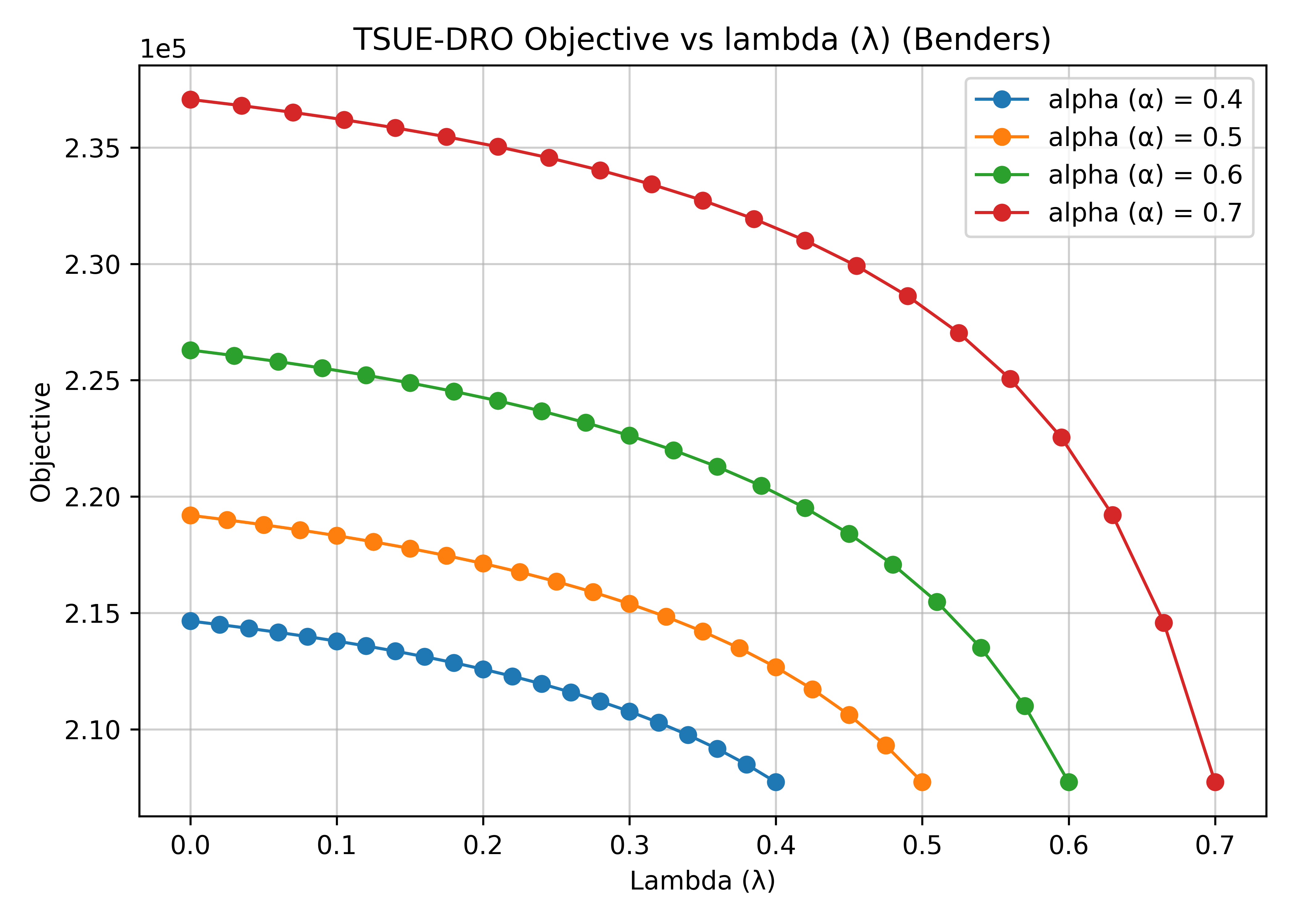
Figure 13 illustrates convergence and runtime for $(\alpha,\lambda)=(0.4,0.2)$. The bounds converge in 437 iterations to an objective of $212578.442$, with most of the gap closed in the first $\approx 60$ cuts. Compared to solving the SOCP using cvxpy/splitting conic solver (SCS), Benders is faster at larger scales (e.g., 3.8s vs 7.5s at 6,000 travelers per OD), comparable around 3,000 travelers (both $\approx$2s), and faster again at 2,000 travelers. Figure 14 supports Propositions 4.1–4.3. The TSUE-DRO objective decreases monotonically in $\lambda$ for each $\alpha\in\{0.4,0.5,0.6,0.7\}$. For the same $\alpha$ and $\lambda$, TSUE-DRO always yields a higher objective value than TSUE-SP.

Figure 14: Objective value vs. $\boldsymbol{\lambda}$. The left panel reports the objective function under TSUE-SP (Approach B2); the right panel reports the objective function under the stationary TSUE-DRO.

Tables 5–6 in appendix S show analogous but less sensitive to parameters patterns under stationary TSUE-DRO. OD (c2,a3) flow splits mainly between Path 6 (47.4%–49.3%) and Path 7 (28.0%–28.9%), OD (c3,a3) flow remains almost entirely on Path 11 (98.4%–98.6%), and OD (c1,a3) flow is still mainly using Path 17 (about 52%). With $\alpha=0.40$, reducing $\lambda$ from $0.30$ to $0.10$ produces modest rerouting that strengthens the corridor a2$\rightarrow$a3 (4294.9$\rightarrow$4320.3 veh/h) use and reduces use of b3$\rightarrow$a3 (7705.1$\rightarrow$7679.7 veh/h). Varying $\alpha$ at $\lambda=0.30$ changes flows only moderately and results in flow on long detours at low volumes.

Comparing TSUE-SP and TSUE-DRO, distributional robustness shifts flow toward reliable radial links and reduces sensitivity to $(\alpha,\lambda)$. Under $(\alpha,\lambda)=(0.40,0.30)$, link a2$\rightarrow$a3 carries $2946.9$ veh/h in SP versus $4294.9$ veh/h in DRO (+45.74%), while b3$\rightarrow$a3 decreases from $9053.1$ to $7705.1$ veh/h (-17.49%). Link flows also vary less under parameter perturbation, consistent with the stabilizing effect of the Wasserstein ambiguity set.

8 Conclusion

We extend the TSUE framework by integrating tail risk quantification with behavioral route choice, supporting resilient transportation planning through the confidence level and the risk aversion weight. To reduce sensitivity to these parameters, we propose path-based and potential-based TSUE-SP formulations and establish the conditions under which they are equivalent. We further develop TSUE-DRO under stationary and non-stationary cases within the 1-Wasserstein ambiguity ball, and derive a Benders decomposition algorithm to solve the resulting model.

Numerical experiments in a stylized (3 $\times$ 3) transportation network in downtown Chicago, IL show consistent responses across explicit hazard scenarios, TSUE-SP, and TSUE-DRO, with higher risk sensitivity shifting flow away from hazard-prone bottlenecks toward more reliable corridors. The results also indicate that distributional robustness based on Wasserstein ambiguity strengthens and stabilizes this traffic flow redistribution by reducing sensitivity to extreme parameter choices. Computationally, we develop a tailored Benders decomposition algorithm that solves TSUE-DRO instances within 400 iterations and reduces runtime to roughly half of that required by SCS.

Future research should explore scaling this approach to larger transportation networks through advanced computational methods, such as Benders decomposition with partitioned parallelism or column generation with on-demand path addition.

This research was partially supported by the Clean Energy and Equitable Transportation Solutions (CLEETS) NSF-UKRI Global Center, under NSF award no. 2330565, and the NSF CAREER award no. 2237881.

Appendix A Parameters

In this Appendix, we present the mathematical notation in Table LABEL:tab:notation.

Table 1: Nomenclature

Symbol	Type	Description	Symbol	Type	Description
Network and paths
$G=(V,E)$	Graph	Directed transportation network	$V$	Set	Nodes
$E$	Set	Directed links (arcs)	$a$	Index	Link index
$(o,d)$	Indices	OD pair	$K_{od}$	Set	Candidate paths for $(o,d)$
$k$	Index	Path index	$\delta_{a,k}^{od}$	Parameter	Link–path incidence (0/1)
Flows and demand
$q_{od}$	Parameter	OD demand	$f_{k}^{od}$	Decision var.	Path flow
$f$	Decision vec.	All path flows	$x_{a}$	Decision var.	Link flow
$f^{w}$	Decision var.	Regime-specific flow vector (Scenario B)
Uncertainty and scenarios
$\xi_{a}$	Random var.	Link operating state	$\xi$	Random vec.	Network state (all links)
$s$	Index	Scenario index	$S$	Parameter	Number of scenarios
$\xi^{s}$	Realization	Scenario realization	$p_{s}$	Parameter	Scenario probability weight
$p_{a}^{s}$	Parameter	Link-level scenario probability	$\mathbb{E}[\cdot]$	Operator	Expectation
Link travel time (extended BPR)
$t_{a}(\cdot,\xi_{a})$	Function	Link travel time under $\xi_{a}$	$t_{a}^{s}(\cdot)$	Function	Scenario-$s$ link travel time
$t_{a}^{0}(\xi_{a})$	Parameter	Free-flow time (state-dependent)	$c_{a}(\xi_{a})$	Parameter	Capacity (state-dependent)
$\alpha(\xi_{a})$	Parameter	BPR coefficient (not CVaR $\alpha$)	$\beta(\xi_{a})$	Parameter	BPR exponent
$\Delta_{a}(\xi_{a})$	Parameter	Fixed delay (state-dependent)
Path travel time and truncated logit
$t_{k}^{od}(v,\xi)$	Random var.	Random path travel time	$t_{k}^{od,s}(v)$	Function	Scenario-$s$ path travel time
$\phi_{k}^{od}(v)$	Function	Deterministic path cost in kernel	$\phi_{k,\alpha,\lambda}^{od}(v)$	Function	Risk-adjusted path cost (Approach A)
$\theta$	Parameter	Logit time sensitivity / scale	$\pi_{od}$	Parameter	Truncation (feasibility) cutoff
$P_{k}^{od}$	Probability	Truncated-logit choice probability	$[x]_{+}$	Operator	Positive part
$U_{k}$	Random var.	Path utility	$\delta_{k}$	Random var.	Gumbel error term
$K_{od}^{\alpha,\lambda}(v)$	Set	Admissible paths under risk screen	$\mu_{od}$	Dual var.	OD conservation multiplier (reservation cost)
$g_{k}^{od}(f)$	Function	Induced risk-adjusted marginal path cost
Potentials and risk measures
$B(v)$	Function	Beckmann congestion potential	$\widehat{Z}^{s}(f)$	Function	Scenario-$s$ congestion potential
$\widehat{Z}(f,\xi)$	Random var.	Random congestion potential	$\Psi(f)$	Function	Entropy regularization term
$Z^{s}(f)$	Function	Scenario-$s$ TSUE potential	$Z(f,\xi)$	Random var.	Random TSUE potential
$\operatorname{VaR}_{\alpha}(\cdot)$	Risk measure	Value-at-Risk (interpretation)	$\operatorname{CVaR}_{\alpha}(\cdot)$	Risk measure	Conditional Value-at-Risk
$\alpha$	Parameter	CVaR confidence level	$\lambda$	Parameter	Behavioral tail-sensitivity parameter
$\bar{\lambda}(\alpha,\lambda)$	Parameter	Effective mixing weight (normalized CE)	$\Phi_{\alpha,\lambda}(\cdot)$	Function	Normalized mean–CVaR certainty equivalent
$\tau_{\alpha}(\cdot)$	Function	Buffer vs. mean-excess indicator	$M$	Parameter	Large penalty / upper bound for extreme delay
CVaR auxiliary variables and tail weights
$\gamma$ (or $t$)	Aux. var.	CVaR threshold (RU/epigraph)	$u_{s}$	Aux. var.	Scenario excess (system-level)
$\gamma_{k}^{od}$	Aux. var.	Path-level CVaR threshold	$u_{k,s}^{od}$	Aux. var.	Path-level scenario excess
$\chi_{s}$	Aux. var.	Tail weight in CVaR subgradient	$\chi_{s}^{\alpha}$	Parameter	Canonical tail weights (ordered scenarios)
$F(m)$	Function	Cumulative scenario probability	$m(\alpha)$	Parameter	VaR index in ordered scenarios
$\widetilde{p}_{s}$	Parameter	Distorted scenario probabilities (regime dominance)	$\tau_{k}^{od,s}(v)$	Function	Scenario-$s$ marginal path time
Wasserstein DRO (stationary)
$P_{0}$	Distribution	Empirical distribution of $\xi$	$\widehat{P}$	Distribution	Unknown true distribution
$Q$	Distribution	Alternative law in ambiguity set	$\mathcal{D}$	Set	Wasserstein ambiguity set
$W_{1}(Q,P_{0})$	Metric	1-Wasserstein distance	$\rho$	Parameter	Wasserstein radius
$d(\cdot,\cdot)$	Function	Ground metric (not destination $d$)	$\|\cdot\|_{2}$	Operator	Euclidean norm
$\Pi(Q,P_{0})$	Set	Coupling (transport plan) set	$\pi$	Measure	A coupling in $\Pi(Q,P_{0})$
$\Xi$	Set	Support of $\xi$	$m$	Parameter	Dimension of $\xi$
Finite-sample calibration
$N$	Parameter	Number of samples	$\delta$	Parameter	Confidence parameter
$\rho_{N,\delta}$	Parameter	Finite-sample radius	$\nu$	Parameter	Light-tail exponent
$A$	Parameter	Moment constant	$c_{1},c_{2}$	Parameters	Concentration constants
DRO dual / SOCP / cutting planes
$g_{t}(f,\xi)$	Function	Hinge-augmented payoff (dual)	$\kappa$	Aux. var.	Wasserstein dual variable
$s_{i}$	Aux. var.	Epigraph variable (sample $i$)	$\xi^{i}$	Sample	Empirical sample $i$
$Z_{0}(f)$	Function	Affine-in-$\xi$ intercept	$h(f)$	Function	Affine-in-$\xi$ coefficient vector
$a_{0}(f),b_{0}(f)$	Functions	First affine piece (SOCP case)	$a_{1}(f),b_{1}(f,t)$	Functions	Second affine piece (SOCP case)
$r$	Index	Exchange/Benders iteration	$\mathcal{X}_{i}^{(r)}$	Set	Active support subset at iter. $r$
$\Delta_{i}^{(r)}$	Quantity	Separation violation	$\xi_{i}^{\star}$	Point	Maximizer added as a cut
Regime-dependent (structured) ambiguity sets
$W$	Random var.	Regime indicator	$\mathcal{W}_{F}$	Set	Regime set (e.g., NR/HR/FL)
$p_{w}$	Parameter	Regime probability	$N_{w}$	Parameter	Samples in regime $w$
$P_{0}^{w}$	Distribution	Regime empirical distribution	$\mathcal{D}^{w}$	Set	Regime Wasserstein ball
$Q^{w}$	Distribution	Regime alternative distribution	$\rho_{w}$	Parameter	Regime Wasserstein radius
$\mathcal{D}_{\mathrm{str}}$	Set	Structured ambiguity set	$\Xi_{w}$	Set	Regime support (often $\Xi$)
$\kappa_{w}$	Aux. var.	Regime Wasserstein dual variable	$s_{w,i}$	Aux. var.	Regime epigraph variable
$t_{w}$	Aux. var.	Regime CVaR threshold (Scenario B)	$\delta_{w}$	Parameter	Regime confidence split (union bound)

Appendix B Derivation of truncated logit formula via KKT conditions

For an OD pair $(o,d)$ with demand $q_{od}$ and paths $K_{od}$, let $f_{k}^{od}\geq 0$ denote the flow on path $k$, and $c_{k}^{od}$ the perceived cost. The optimization problem then is as follows:

$$\min_{\left\{f_{k}^{od}\geq 0\right\}}\left[\sum_{k\in K_{od}}c_{k}^{od}f_{k}^{od}+\frac{1}{\theta}\sum_{k\in K_{od}}\left\{\left(f_{k}^{od}+1\right)\ln\left(f_{k}^{od}+1\right)-f_{k}^{od}\right\}\right],$$ (63)

subject to: $\sum_{k\in K_{od}}f_{k}^{od}=q_{od},\quad f_{k}^{od}\geq 0$. The Lagrangian is derived as (64):

$$\mathcal{L}=\sum_{k}c_{k}f_{k}+\frac{1}{\theta}\sum_{k}\left[\left(f_{k}+1\right)\ln\left(f_{k}+1\right)-f_{k}\right]+\lambda\left(q_{rs}-\sum_{k}f_{k}\right)+\sum_{k}\mu_{k}\left(-f_{k}\right),$$ (64)

with $\lambda$ and $\mu_{k}\geq 0$ as Lagrange multipliers. The KKT conditions include:

The KKT conditions characterize the optimum as follows. Stationarity requires $\frac{\partial\mathcal{L}}{\partial f_{k}}=c_{k}+\frac{1}{\theta}\ln\left(f_{k}+1\right)-\lambda-\mu_{k}=0$. Primal feasibility imposes $\sum_{k}f_{k}=q_{od}$ and $f_{k}\geq 0$. Dual feasibility requires $\mu_{k}\geq 0$. Complementary slackness demands $\mu_{k}f_{k}=0$. For $f_{k}>0$, we have $\mu_{k}=0$, which shows:

$$c_{k}+\frac{1}{\theta}\ln\left(f_{k}+1\right)=\lambda\Rightarrow f_{k}=\exp\left[\theta\left(\lambda-c_{k}\right)\right]-1$$ (65)

If $\exp\left[\theta\left(\lambda-c_{k}\right)\right]-1<0$, then $f_{k}=0$. Thus, $f_{k}=\max\left\{0,\exp\left[\theta\left(\lambda-c_{k}\right)\right]-1\right\}$. Satisfying demand requires $\sum_{k}\max\left\{0,\exp\left[\theta\left(\lambda-c_{k}\right)\right]-1\right\}=q_{rs}$. Setting $\lambda=-\theta\pi_{od}$, the flow becomes:

$$f_{k}=\max\left\{0,\exp\left[-\theta\left(c_{k}-\pi_{od}\right)\right]-1\right\}.$$ (66)

Finally, the choice probability is:

$$P_{k}^{rs}=\frac{\left[\exp\left(-\theta\left(c_{k}-\pi_{od}\right)\right)-1\right]_{+}}{\sum_{\ell}\left[\exp\left(-\theta\left(c_{\ell}-\pi_{od}\right)\right)-1\right]_{+}}.$$ (67)

Appendix C Proof of Proposition 2.1

First, the BPR function (as in Eq. (1)) is known to be convex and so is the summation $\sum_{a\in A}\int_{0}^{x_{a}}t_{a}(\omega)\mathrm{d}\omega$ in $x_{a}$, as the integral of a convex function is convex. Then, we consider the entropy term in the objective function $\frac{1}{\theta}\sum_{o,d}\sum_{k\in K_{od}}\left[\left(f_{k}^{od}+1\right)\ln\left(f_{k}^{od}+1\right)-f_{k}^{od}\right]$. Consider the function $g(f)=(f+1)\ln(f+1)-f$. Its first derivative is: $g^{\prime}(f)=\ln(f+1)+\frac{f+1}{f+1}-1=\ln(f+1)$. Similarly, the second derivative can be computed as $g^{\prime\prime}(f)=\frac{1}{f+1}>0$ for $f\geq 0$. Thus, $g(f)$ is strictly convex. Finally, the expectation of the summation of the two parts is also strictly convex in $f_{k}^{od}$. Overall, the objective is strictly convex. For the second part of the proposition, we derive the Lagrangian as in (68):

$$\mathcal{L} =\mathbb{E}\left[\sum_{a\in A}\int_{0}^{x_{a}}t_{a}(\omega,\xi)\mathrm{d}\omega+\frac{1}{\theta}\sum_{0,d}\sum_{k\in K_{od}}\left[\left(f_{k}^{od}+1\right)\ln\left(f_{k}^{od}+1\right)-f_{k}^{od}\right]\right]+\lambda\left(q_{od}-\sum_{k}f_{k}\right)+\sum_{k}\mu_{k}\left(-f_{k}\right)$$ (68)

$$=\mathbb{E}\left[\sum_{a\in A}\int_{0}^{x_{a}}t_{a}(\omega,\xi)\mathrm{d}\omega\right]+\frac{1}{\theta}\sum_{0,d}\sum_{k\in K_{od}}\left[\left(f_{k}^{od}+1\right)\ln\left(f_{k}^{od}+1\right)-f_{k}^{od}\right]+\lambda\left(q_{od}-\sum_{k}f_{k}\right)+\sum_{k}\mu_{k}\left(-f_{k}\right),$$

with $\lambda$ and $\mu_{k}\geq 0$ as the Lagrange multipliers. Using $x_{a}=\sum_{l}\delta_{al}f_{l}$ and the chain rule, we have:

$$\frac{\partial\mathcal{L}}{\partial f_{k}}=\mathbb{E}\left[\sum_{a}t_{a}\left(x_{a},\xi\right)\delta_{ak}\right]+\frac{1}{\theta}\ln\left(f_{k}+1\right)-\lambda-\mu_{k},\quad\frac{\partial\mathcal{L}}{\partial\lambda}=q_{od}-\sum_{k}f_{k},\quad\frac{\partial\mathcal{L}}{\partial\mu_{k}}=-f_{k}.$$ (69)

We can then produce the Hessian with ordering $(f,\lambda,\mu)$. For any two paths $k$ and $l$, we have:

$$\frac{\partial^{2}\mathcal{L}}{\partial f_{k}\partial f_{l}}=\mathbb{E}\left[\sum_{a}t_{a}^{\prime}\left(x_{a},\xi\right)\delta_{ak}\delta_{al}\right]+\frac{1}{\theta}\frac{\delta_{kl}}{f_{k}+1}.$$ (70)

The first term in Eq. (70) collects together any two paths that share at least one common link. The second term, corresponding to entropy, is diagonal and strictly positive. Except for these two terms, we also have mixed derivatives with multipliers:

$$\frac{\partial^{2}\mathcal{L}}{\partial f_{k}\partial\lambda}=\frac{\partial^{2}\mathcal{L}}{\partial\lambda\partial f_{k}}=-1,\quad\frac{\partial^{2}\mathcal{L}}{\partial f_{k}\partial\mu_{l}}=\frac{\partial^{2}\mathcal{L}}{\partial\mu_{l}\partial f_{k}}=-\delta_{kl},$$ (71)

as well as the remaining blocks in the form of $\frac{\partial^{2}\mathcal{L}}{\partial\lambda^{2}}=0,\frac{\partial^{2}\mathcal{L}}{\partial\lambda\partial\mu_{k}}=0,\frac{\partial^{2}\mathcal{L}}{\partial\mu_{k}\partial\mu_{l}}=0$.

Let $T$ be a square matrix with elements $T_{kl}=\mathbb{E}\left[\sum_{a}t_{a}^{\prime}\left(x_{a},\xi\right)\delta_{ak}\delta_{al}\right]$ , and $D=\operatorname{diag}\left\{\frac{1}{\theta\left(f_{k}+1\right)}\right\}$. Define $H_{ff}=T+D$. Finally, the Hessian is:

$$\nabla^{2}\mathcal{L}=\left[\begin{array}[]{ccc}H_{ff}&-\mathbf{1}&-I\\ -\mathbf{1}^{\top}&0&0\\ -I&0&0\end{array}\right],$$ (72)

where $\mathbf{1}$ and $I$ are suitably dimensioned vectors of ones and identity matrices.

If each cost function satisfies $t_{a}^{\prime}\left(x_{a},\xi\right)\geq 0$, then $T\succeq 0$ and the diagonal matrix $D\succ 0$, which implies that $H_{ff}\succ 0$. Hence, the Lagrangian is strictly convex in the flows (for fixed multipliers), which guarantees uniqueness of the expectation of the TSUE path flow vector.

Appendix D Misleading Truncation Under Expectation-Based Example

For example, expectation-based truncation can be misleading in heavy-tailed or mixture settings: for any fixed $\pi_{od}>0$ and any small $\varepsilon>0$, define a travel time random variable

$$T=\begin{cases}\pi_{od}+\varepsilon,&\text{w.p. }1-\delta,\\ 0,&\text{w.p. }\delta,\end{cases}\qquad\text{with}\qquad\delta>\frac{\varepsilon}{\pi_{od}+\varepsilon}.$$ (73)

Then, $\mathbb{E}[T]=(1-\delta)(\pi_{od}+\varepsilon)<\pi_{od}$ so the path remains admissible under $K_{od}^{\mathrm{TL}}(v)$, while $\mathbb{P}(T>\pi_{od})=1-\delta$ can approach $1$ by setting $\varepsilon$ sufficiently small. Thus, when $\phi_{k}^{od}(v)$ uses expectation alone, the truncated logit assesses paths by mean performance rather than service reliability. This is problematic in hazard-prone networks, where disruption regimes generate frequent threshold exceedance despite low unconditional means.

Appendix E Proof of Proposition 3.1

Define two mutually exclusive and collectively exhaustive events: $A=\left\{Z(f,\xi)\leq\operatorname{VaR}_{\alpha}(Z(f,\xi))\right\}$ with probability $P(A)=\alpha$, and $B=\left\{Z(f,\xi)>\operatorname{VaR}_{\alpha}(Z(f,\xi))\right\}$ with probability $P(B)=1-\alpha$. By the law of total expectation $\mathbb{E}[Z(f,\xi)]=\mathbb{E}[Z(f,\xi)\mid A]\cdot P(A)+\mathbb{E}[Z(f,\xi)\mid B]\cdot P(B)$. Substituting the probabilities yields:

$$\mathbb{E}[Z(f,\xi)]=\mathbb{E}\left[Z(f,\xi)\mid Z(f,\xi)\leq\operatorname{VaR}_{\alpha}(Z(f,\xi))\right]\cdot\alpha+\mathbb{E}\left[Z(f,\xi)\mid Z(f,\xi)>\operatorname{VaR}_{\alpha}(Z(f,\xi))\right]\cdot(1-\alpha).$$ (74)

By definition, $\mathbb{E}\left[Z(f,\xi)\mid Z(f,\xi)>\operatorname{VaR}_{\alpha}(Z(f,\xi))\right]=\operatorname{CVaR}_{\alpha}(Z(f,\xi))$. Thus:

$$\mathbb{E}[Z(f,\xi)]=\mathbb{E}\left[Z(f,\xi)\mid Z(f,\xi)\leq\operatorname{VaR}_{\alpha}(Z(f,\xi))\right]\cdot\alpha+\operatorname{CVaR}_{\alpha}(Z(f,\xi))\cdot(1-\alpha).$$ (75)

Note that $\mathbb{E}\left[Z(f,\xi)\mid Z(f,\xi)\leq\operatorname{VaR}_{\alpha}(Z(f,\xi))\right]$ represents the expected value in the better $\alpha$ fraction (lower travel times), while $\operatorname{CVaR}_{\alpha}(Z(f,\xi))$ represents the expected value in the worse $1-\alpha$ fraction (higher travel times due to hazards). Since $Z$ is a cost variable, values in $B$ exceed those in $A$. Therefore, $\mathbb{E}\left[Z(f,\xi)\mid Z(f,\xi)\leq\operatorname{VaR}_{\alpha}(Z(f,\xi))\right]\leq\operatorname{VaR}_{\alpha}(Z(f,\xi))\leq\operatorname{CVaR}_{\alpha}(Z(f,\xi))$. Rearranging the total expectation equation:

$$\operatorname{CVaR}_{\alpha}(Z(f,\xi))\cdot(1-\alpha)=\mathbb{E}[Z(f,\xi)]-\mathbb{E}\left[Z(f,\xi)\mid Z(f,\xi)\leq\operatorname{VaR}_{\alpha}(Z(f,\xi))\right]\cdot\alpha.$$ (76)

The subtracted term is nonnegative and at most equal to $\mathbb{E}[Z(f,\xi)]$. Thus, $\operatorname{CVaR}_{\alpha}(Z(f,\xi))\geq\mathbb{E}[Z(f,\xi)]$, with equality holding if and only if $Z$ is constant. Given that hazards cause variability, $Z$ is not constant, leading to $\operatorname{CVaR}_{\alpha}(Z(f,\xi))>\mathbb{E}[Z(f,\xi)]$, which completes the proof.

Appendix F Proof of Proposition 3.3

If a random travel time $\tilde{Z}$ is absolutely continuous (has a pdf), then $\mathbb{P}(\tilde{Z}=M)=0$ for any fixed $M$. However, in the truncated simulation, it is able to impose an operational cap/penalty (time-out, infeasibility penalty), which censors the realized cost at a finite upper bound $M$. Define $Z:=\min(\tilde{Z},\,M)$. Even when $\tilde{Z}$ is continuous, the capped variable $Z$ has an atom at $M$: $\mathbb{P}(Z=M)\;=\;\mathbb{P}(\tilde{Z}\geq M)$, which can be strictly positive. Define $\Psi(\gamma):=\gamma+\frac{1}{1-\alpha}\mathbb{E}\bigl[(Z-\gamma)_{+}\bigr]$ as in (8). Since $Z\leq M$ a.s., if $\gamma\geq M$ then $(Z-\gamma)_{+}=0$ a.s., hence $\Psi(\gamma)=\gamma\geq M$. In particular, $\Psi(M)=M$, which implies $\inf_{\gamma\in\mathbb{R}}\Psi(\gamma)\leq M$.

If $\gamma<M$, then on the event $\{Z=M\}$ we have $(Z-\gamma)_{+}=M-\gamma$, and therefore

$$\mathbb{E}\bigl[(Z-\gamma)_{+}\bigr]\;\geq\;\mathbb{E}\bigl[(Z-\gamma)_{+}\,\mathbf{1}_{\{Z=M\}}\bigr]=(M-\gamma)\mathbb{P}(Z=M)\;\geq\;(M-\gamma)(1-\alpha),$$ (77)

where the last inequality uses the assumption $\mathbb{P}(Z=M)\geq 1-\alpha$. It follows that

$$\Psi(\gamma)\;\geq\;\gamma+\frac{1}{1-\alpha}(M-\gamma)(1-\alpha)=M.$$ (78)

Thus $\Psi(\gamma)\geq M$ for all $\gamma\in\mathbb{R}$, implying $\inf_{\gamma\in\mathbb{R}}\Psi(\gamma)\geq M$. Combining with $\inf_{\gamma\in\mathbb{R}}\Psi(\gamma)\leq M$ yields $\inf_{\gamma\in\mathbb{R}}\Psi(\gamma)=M,$ i.e., $\operatorname{CVaR}_{\alpha}(Z)=M$.

Finally, the above argument depends only on the cap $Z\leq M$ a.s. and the mass condition $\mathbb{P}(Z=M)\geq 1-\alpha$, and therefore $\operatorname{CVaR}_{\alpha}(Z)$ is independent of the distribution of $Z$ on $\{Z<M\}$.

Appendix G Proof of Proposition 4.1

Fix $\alpha\in(0,1)$ and a feasible $f$. Let $\mu(f):=\mathbb{E}[Z(f,\xi)]$, and $C_{\alpha}(f):=\operatorname{CVaR}_{\alpha}(Z(f,\xi))$. Under the normalized certainty equivalent used in the paper, for $\lambda\leq\alpha$ we have:

$$\Phi_{\alpha,\lambda}(f)=(1-\bar{\lambda}(\alpha,\lambda))\,\mu(f)+\bar{\lambda}(\alpha,\lambda)\,C_{\alpha}(f),\qquad\bar{\lambda}(\alpha,\lambda)=\frac{\alpha-\lambda}{1+\alpha-2\lambda}.$$ (79)

Since $\alpha$ is fixed, both $\mu(f)$ and $C_{\alpha}(f)$ are constants with respect to $\lambda$. Rewrite $\Phi_{\alpha,\lambda}(f)=\mu(f)+\bar{\lambda}(\alpha,\lambda)\big(C_{\alpha}(f)-\mu(f)\big)$. By Proposition 3.1, $C_{\alpha}(f)-\mu(f)\geq 0$. Moreover,

$$\frac{\partial}{\partial\lambda}\bar{\lambda}(\alpha,\lambda)=\frac{\alpha-1}{(1+\alpha-2\lambda)^{2}}<0\qquad(\text{since }\alpha<1).$$ (80)

Therefore,

$$\frac{\partial}{\partial\lambda}\Phi_{\alpha,\lambda}(f)=\big(C_{\alpha}(f)-\mu(f)\big)\,\frac{\partial}{\partial\lambda}\bar{\lambda}(\alpha,\lambda)\ \leq\ 0,$$ (81)

which proves that $\Phi_{\alpha,\lambda}(f)$ is non-increasing in $\lambda$ for fixed $\alpha$.

Appendix H Proof of Proposition 4.3

Fix $\lambda\in[0,1)$ and consider $\alpha_{2}>\alpha_{1}$ with $\lambda<\alpha_{1}<\alpha_{2}<1$ (risk-averse region). Let

$$\mu(f):=\mathbb{E}[Z(f,\xi)],\qquad C_{i}(f):=\operatorname{CVaR}_{\alpha_{i}}(Z(f,\xi)),\quad i\in\{1,2\}.$$ (82)

Define $\bar{\lambda}_{i}:=\bar{\lambda}(\alpha_{i},\lambda)=\frac{\alpha_{i}-\lambda}{1+\alpha_{i}-2\lambda}$. Then $\bar{\lambda}_{2}\geq\bar{\lambda}_{1}$ because $\frac{\partial}{\partial\alpha}\bar{\lambda}(\alpha,\lambda)=\frac{1-\lambda}{(1+\alpha-2\lambda)^{2}}>0.$ $\operatorname{CVaR}_{\alpha}(\cdot)$ is non-decreasing in $\alpha$, hence $C_{2}(f)\geq C_{1}(f)$. Under the normalized certainty equivalent,

$$\Phi_{\alpha_{i},\lambda}(f)=(1-\bar{\lambda}_{i})\mu(f)+\bar{\lambda}_{i}C_{i}(f),\quad i=1,2.$$ (83)

Compute the difference:

$$\Phi_{\alpha_{2},\lambda}(f)-\Phi_{\alpha_{1},\lambda}(f)=(1-\bar{\lambda}_{2})\mu+\bar{\lambda}_{2}C_{2}-(1-\bar{\lambda}_{1})\mu-\bar{\lambda}_{1}C_{1}=\bar{\lambda}_{2}(C_{2}-C_{1})+(\bar{\lambda}_{2}-\bar{\lambda}_{1})(C_{1}-\mu).$$

Each term on the right-hand side is nonnegative:

$$\bar{\lambda}_{2}\geq 0,\ \ C_{2}-C_{1}\geq 0,\qquad\bar{\lambda}_{2}-\bar{\lambda}_{1}\geq 0,\ \ C_{1}-\mu\geq 0$$ (84)

(where $C_{1}-\mu\geq 0$ follows from Proposition 3.1). Thus $\Phi_{\alpha_{2},\lambda}(f)\geq\Phi_{\alpha_{1},\lambda}(f)$, proving that $\Phi_{\alpha,\lambda}(f)$ is non-decreasing in $\alpha$ for $\lambda<\alpha$.

Appendix I Proof of Proposition 4.5 (Explicit reduction from B1 to the B2 single-level program)

Proof I.1

Proof. Let $\mathcal{F}$ denote the feasible path-flow set induced by (4b)–(4d). Since the demand conservation constraints are affine and the nonnegativity constraints are convex, $\mathcal{F}$ is convex. Moreover, because each OD demand $q_{od}$ is finite, $\mathcal{F}$ is bounded and closed.

First consider Approach B2. By the link-flow relation in (4c), the link-flow vector is an affine function of the path-flow vector $f$. Since each $t_{a}^{s}(\cdot)$ is nondecreasing, the corresponding Beckmann integral is convex in the link flow. Hence, for every scenario $s$, the scenario congestion potential appearing in (26) is convex in $f$.

The expectation part of (26) is a nonnegative weighted sum of convex scenario potentials, and is therefore convex. The CVaR part is also convex in $f$ by the Rockafellar–Uryasev representation in (28): the RU constraints define the epigraph of convex scenario-potential functions, and partial minimization over the auxiliary variables preserves convexity. Since $\bar{\lambda}(\alpha,\lambda)\in[0,1]$, the certainty-equivalent congestion term in (26) is convex in $f$.

Now consider the entropy term defined in (22). For the scalar function

$$h(y)=(y+1)\ln(y+1)-y,\qquad y\geq 0,$$

we have

$$h^{\prime\prime}(y)=\frac{1}{y+1}>0.$$

Therefore, the entropy term in (22) is strictly convex in $f$. Since $\theta>0$, the regularization term $\frac{1}{\theta}\Psi(f)$ is also strictly convex. Consequently, the B2 objective in (27) is the sum of a convex certainty-equivalent congestion term and a strictly convex entropy term. Hence the B2 objective is strictly convex on $\mathcal{F}$.

Because the B2 objective is continuous and $\mathcal{F}$ is compact, an optimal solution exists. Since the objective is strictly convex on the convex set $\mathcal{F}$, the optimal path-flow vector for Approach B2 is unique.

It remains to show that Approach B1 has the same path-flow solution. By (23), the total scenario TSUE potential in B1 differs from the scenario congestion potential by the entropy term $\frac{1}{\theta}\Psi(f)$, which is deterministic with respect to the scenario index. Therefore, using the translation equivariance of expectation and CVaR, the B1 certainty-equivalent objective in (24) satisfies

$$\Phi_{\alpha,\lambda}^{\mathrm{B1}}(f)=\Phi_{\alpha,\lambda}^{\mathrm{B2}}(f)+\frac{1}{\theta}\Psi(f).$$

The right-hand side is exactly the B2 objective in (27). Thus Approaches B1 and B2 have the same reduced objective function in the path-flow vector $f$.

Since the B2 reduced objective is strictly convex and B1 has the same reduced objective, the B1 objective is also strictly convex in $f$. Therefore B1 also has a unique optimal path-flow vector. Moreover, because the two reduced objectives are identical in $f$, the unique B1 and B2 path-flow solutions are the same.

Appendix J Proof of Proposition 4.7

We show that the single-level formulation (e.g., (35a) for Approach B2, and (25a) for Approach B1) is a convex program and can be solved with standard TSUE/SUE machinery augmented by the RU auxiliary variables.

Consider Approach B2 for concreteness. Under discrete scenarios $\{\xi^{s}\}_{s=1}^{S}$ with probabilities $p_{s}$, the risk-averse objective is

$$(1-\bar{\lambda})\sum_{s=1}^{S}p_{s}\,\widehat{Z}^{s}(f)+\bar{\lambda}\,\operatorname{CVaR}_{\alpha}(\widehat{Z}(f,\xi))+\frac{1}{\theta}\Psi(f),\qquad\bar{\lambda}=\bar{\lambda}(\alpha,\lambda)\in[0,1].$$ (85)

Using the RU representation of CVaR, we introduce one scalar $\gamma\in\mathbb{R}$ and one nonnegative slack variable $u_{s}\geq 0$ for each scenario, together with linear constraints $u_{s}\geq\widehat{Z}^{s}(f)-\gamma,\qquad u_{s}\geq 0,\quad s=1,\ldots,S.$ This yields the equivalent single-level objective

$$(1-\bar{\lambda})\sum_{s=1}^{S}p_{s}\,\widehat{Z}^{s}(f)+\bar{\lambda}\,\gamma+\frac{\bar{\lambda}}{1-\alpha}\sum_{s=1}^{S}p_{s}\,u_{s}+\frac{1}{\theta}\Psi(f),$$ (86)

subject to the above RU constraints and the standard TSUE feasibility constraints (4b)–(4d).

Convexity follows because each scenario congestion potential $\widehat{Z}^{s}(f)=\sum_{a\in A}\int_{0}^{x_{a}}t_{a}^{s}(\omega)\,d\omega$ is convex in $f$ (via the linear link-flow mapping and convexity of the Beckmann integrals), the entropy term $\Psi(f)$ is convex, and the RU constraints define an epigraph of a convex function. No integer or binary variables are required. Consequently, the resulting formulation is a single-level convex stochastic program solvable with standard convex optimization methods and TSUE algorithms (e.g., projected descent / MSA / decomposition), with the only additional elements being the auxiliary variables $(\gamma,u_{s})$ and the linear RU constraints.

Appendix K Proof of Proposition 5.1

For any $Q$, linearity of expectation gives $\mathbb{E}_{Q}[Y+b]=\mathbb{E}_{Q}[Y]+b$. Moreover, CVaR is translation invariant with respect to constant shifts: $\operatorname{CVaR}_{\alpha,Q}(Y+b)=\operatorname{CVaR}_{\alpha,Q}(Y)+b$ (e.g., from the RU representation by the change of variables $t\mapsto t-b$). Substituting these identities into the left-hand side of (43) shows that the expression inside the supremum equals $(1-\bar{\lambda})\mathbb{E}_{Q}[Y]+\bar{\lambda}\,\operatorname{CVaR}_{\alpha,Q}(Y)+b$, and taking $\sup_{Q\in\mathcal{D}}$ yields (43). Applying it with $Y(\xi)=\widehat{Z}(f,\xi)$ and $b=c(f)=\Psi(f)/\theta$ yields (44).

Appendix L Proof of Proposition 5.4

Fix a feasible $f$. By the Rockafellar–Uryasev representation, for any distribution $Q$,

$$\operatorname{CVaR}_{\alpha,Q}(Z(f,\xi))=\inf_{t\in\mathbb{R}}\left\{t+\frac{1}{1-\alpha}\mathbb{E}_{Q}\big[(Z(f,\xi)-t)_{+}\big]\right\}.$$

Substituting this into the definition of $\Phi_{\alpha,\lambda}^{\mathrm{DRO}}(f)$ gives

$$\Phi_{\alpha,\lambda}^{\mathrm{DRO}}(f)=\sup_{Q\in\mathcal{D}}\ \inf_{t\in\mathbb{R}}\left\{\bar{\lambda}\,t+\mathbb{E}_{Q}\!\big[g_{t}(f,\xi)\big]\right\},$$

where $g_{t}$ is defined in (47). By the max–min inequality,

$$\sup_{Q\in\mathcal{D}}\inf_{t\in\mathbb{R}}\{\bar{\lambda}t+\mathbb{E}_{Q}[g_{t}]\}\;\leq\;\inf_{t\in\mathbb{R}}\sup_{Q\in\mathcal{D}}\{\bar{\lambda}t+\mathbb{E}_{Q}[g_{t}]\}=\inf_{t\in\mathbb{R}}\left\{\bar{\lambda}t+\sup_{Q\in\mathcal{D}}\mathbb{E}_{Q}[g_{t}(f,\xi)]\right\}.$$

Next, by the Wasserstein dual inequality in (Mohajerin Esfahani and Kuhn 2018, Theorem 4.2) (under Assumption 5.4), for each fixed $t$,

$$\sup_{Q:W_{1}(Q,P_{0})\leq\rho}\ \mathbb{E}_{Q}[g_{t}(f,\xi)]\;\leq\;\inf_{\kappa\geq 0}\left\{\kappa\rho+\mathbb{E}_{P_{0}}\!\left[\sup_{\xi\in\Xi}\big(g_{t}(f,\xi)-\kappa\|\xi-\xi_{0}\|_{2}\big)\right]\right\}.$$

Specializing to $P_{0}=\frac{1}{N}\sum_{i=1}^{N}\delta_{\xi^{i}}$ yields

$$\sup_{Q:W_{1}(Q,P_{0})\leq\rho}\ \mathbb{E}_{Q}[g_{t}(f,\xi)]\;\leq\;\inf_{\kappa\geq 0}\left\{\kappa\rho+\frac{1}{N}\sum_{i=1}^{N}\sup_{\xi\in\Xi}\big(g_{t}(f,\xi)-\kappa\|\xi-\xi^{i}\|_{2}\big)\right\}.$$

Combining the last two displays and minimizing over $t$ proves (48). Finally, if (i) the minimax interchange holds for the epigraph form and (ii) the piecewise-concave condition of (Mohajerin Esfahani and Kuhn 2018, Assumption 4.1) holds for $g_{t}(f,\cdot)$ on a convex closed $\Xi$, then the max–min inequality and the Wasserstein dual inequality are both tight, so (48) holds with equality. Introducing epigraph variables $s_{i}$ converts the samplewise suprema into the semi-infinite constraints in (49).

Appendix M Pseudocode for Benders Decomposition for 1-Wasserstein TSUE-DRO

Algorithm 1 Benders-type Exchange (Cutting-Plane) Algorithm for $1$-Wasserstein TSUE–DRO

1:empirical samples $\{\xi^{1},\dots,\xi^{N}\}$ (center of $P_{0}$), support set $\Xi$ (or a set of scenarios), radius $\rho$, parameters $(\alpha,\lambda)$ with $\lambda\leq\alpha$, tolerances $\varepsilon_{\mathrm{sep}},\varepsilon_{\mathrm{gap}}$

2:approximate optimal $(f^{\star},t^{\star},\kappa^{\star})$ and corresponding objective value

3:$\bar{\lambda}\leftarrow\bar{\lambda}(\alpha,\lambda)=\dfrac{\alpha-\lambda}{1+\alpha-2\lambda}$;  $g_{t}(f,\xi)\ :=\ (1-\bar{\lambda})\,Z(f,\xi)\;+\;\frac{\bar{\lambda}}{1-\alpha}\bigl(Z(f,\xi)-t\bigr)_{+}\text{(cf.\ \eqref{eq:gt_def})}$.

4:$\mathcal{X}_{i}^{(0)}\leftarrow\{\xi^{i}\}$ for all $i=1,\dots,N$;  $\mathtt{LB}\leftarrow-\infty$, $\mathtt{UB}\leftarrow+\infty$, $k\leftarrow 0$

5:while $\mathtt{UB}-\mathtt{LB}>\varepsilon_{\mathrm{gap}}$ do

6:  (RMP) Solve the restricted main problem with current cut sets $\{\mathcal{X}_{i}^{(k)}\}$:

$$\min_{f,t,\kappa,\{s_{i}\},\{u_{i,\zeta}\}} \bar{\lambda}\,t\;+\;\rho\,\kappa\;+\;\frac{1}{N}\sum_{i=1}^{N}s_{i}$$

s.t. $$s_{i}\ \geq\ (1-\bar{\lambda})\,Z(f,\zeta)\;+\;\frac{\bar{\lambda}}{1-\alpha}\,u_{i,\zeta}\;-\;\kappa\|\zeta-\xi^{i}\|_{2},\qquad u_{i,\zeta}\ \geq\ Z(f,\zeta)-t,\qquad\kappa\geq 0,\qquad\text{\eqref{eq:demand_conservation}--\eqref{eq:nennegative}}.\qquad u_{i,\zeta}\geq 0,\qquad\forall i,\ \forall\zeta\in\mathcal{X}_{i}^{(k)}$$

7:  Let $(f^{k},t^{k},\kappa^{k},s^{k})$ be the optimal solution and set $\mathtt{LB}\leftarrow\bar{\lambda}\,t^{k}+\rho\,\kappa^{k}+\frac{1}{N}\sum_{i=1}^{N}s_{i}^{k}$

8:  (SEP) Separation oracle / violated-cut search: $\Delta_{\max}\leftarrow 0$;  $\widehat{s}_{i}\leftarrow s_{i}^{k}$ for all $i$

9:  for $i=1$ to $N$ do

10:   Solve the separation problem (exactly or approximately):

$$\widehat{s}_{i}\ \leftarrow\ \sup_{\xi\in\Xi}\Big\{g_{t^{k}}(f^{k},\xi)-\kappa^{k}\|\xi-\xi^{i}\|_{2}\Big\},\xi_{i}^{\star}\in\arg\max_{\xi\in\Xi}\Big\{g_{t^{k}}(f^{k},\xi)-\kappa^{k}\|\xi-\xi^{i}\|_{2}\Big\}.$$

11:   Compute violation $\Delta_{i}\leftarrow\widehat{s}_{i}-s_{i}^{k}$ and update $\Delta_{\max}\leftarrow\max\{\Delta_{\max},\Delta_{i}\}$

12:   if $\Delta_{i}>\varepsilon_{\mathrm{sep}}$ then

13:    Add the violated cut by updating $\mathcal{X}_{i}^{(k+1)}\leftarrow\mathcal{X}_{i}^{(k)}\cup\{\xi_{i}^{\star}\}$

14:   else

15:    Do not add any violated cuts and keep $\mathcal{X}_{i}^{(k+1)}\leftarrow\mathcal{X}_{i}^{(k)}$

16:   end if

17:  end for

18:  (UB update) Form a feasible objective value for the original semi-infinite problem by setting $s_{i}=\widehat{s}_{i}$:

$$\mathtt{UB}\ \leftarrow\ \min\left\{\mathtt{UB},\ \bar{\lambda}\,t^{k}+\rho\,\kappa^{k}+\frac{1}{N}\sum_{i=1}^{N}\widehat{s}_{i}\right\}.$$

19:  if $\Delta_{\max}\leq\varepsilon_{\mathrm{sep}}$ then

20:   break $\triangleright$ No violated cuts: $(f^{k},t^{k},\kappa^{k})$ is feasible and optimal (up to tolerance).

21:  end if

22:  $k\leftarrow k+1$

23:end while

24:return $(f^{\star},t^{\star},\kappa^{\star})\leftarrow(f^{k},t^{k},\kappa^{k})$ and objective $\mathtt{UB}$

Appendix N Accelerating the Benders-type exchange method for $1$-Wasserstein TSUE–DRO

This appendix summarizes practical accelerations for the cutting-plane method used to solve the exact semi-infinite reformulation (49) (Algorithm 1). These enhancements reduce the main problem size, separation cost, and iteration count while preserving correctness up to prescribed tolerances.

In the main problem, the hinge $(Z(f,\zeta)-t)_{+}$ does not depend on the sample index $i$. Hence, for each cut point $\zeta$ we use a shared slack variable $u_{\zeta}$ (instead of $u_{i,\zeta}$):

$$u_{\zeta}\geq Z(f,\zeta)-t,\quad u_{\zeta}\geq 0,\qquad\forall\zeta\in\mathcal{X}^{(r)}:=\cup_{i=1}^{N}\mathcal{X}_{i}^{(r)}.$$

Enforcing this for all $i$ and $\zeta\in\mathcal{X}_{i}^{(r)}$ leads to: $s_{i}\geq(1-\bar{\lambda})\,Z(f,\zeta)+\frac{\bar{\lambda}}{1-\alpha}\,u_{\zeta}-\kappa\|\zeta-\xi^{i}\|_{2}.$ This removes an $\mathcal{O}(N)$ increase in auxiliary variables/constraints which can often yield a significant speedup.

Instead of solving the separation problem (53) for all $i=1,\ldots,N$ every iteration, we may evaluate it only for a subset $I^{(r)}$ (e.g., Top-$K$ indices with largest $s_{i}^{(r)}$ or largest $Z(f^{(r)},\xi^{i})$), add violated cuts for $i\in I^{(r)}$, and run a full audit (considering all $i$) periodically, as in every $T$ iterations. This terminates only when a full audit detects no violation. Since separations are independent across $i$ (and across regimes in structured variants), they can be parallelized.

If $Z(f,\cdot)$ is $L_{Z}(f)$-Lipschitz on $\Xi$ under the $\|\cdot\|_{2}$ norm, then $g_{t}(f,\cdot)$ is $L_{g}(f)$-Lipschitz with

$$L_{g}(f)=\Bigl((1-\bar{\lambda})+\frac{\bar{\lambda}}{1-\alpha}\Bigr)L_{Z}(f).$$

Let $D_{i}$ be a bound on $\sup_{\xi\in\Xi}\|\xi-\xi^{i}\|_{2}$. Then

$$\sup_{\xi\in\Xi}\big(g_{t}(f,\xi)-\kappa\|\xi-\xi^{i}\|_{2}\big)\leq g_{t}(f,\xi^{i})+\max\{L_{g}(f)-\kappa,0\}D_{i}.$$

If the right-hand side minus $s_{i}^{(r)}$ is $\leq\varepsilon_{\mathrm{sep}}$, the separation for this $i$ can be safely skipped.

To reduce iterations, use stabilized cutting planes (e.g., a proximal term $\frac{\sigma}{2}\|f-f^{(r-1)}\|_{2}^{2}$ or a trust region) in the main problem. We only add cuts with violation $>\varepsilon_{\mathrm{sep}}$, we periodically prune persistently inactive cuts, and we track an incumbent, best feasible upper-bound solution. When solving multiple instances (e.g., different $\rho$ or $(\alpha,\lambda)$), we can warm-start using both the previous solution and the cut sets. We note that continuation in $\rho$ is particularly effective.

If it is impossible or intractable to maximize exactly (53) (e.g., if using black-box hazard simulators), we instead can use heuristic separation to generate candidate maximizers and add the necessary cuts. The approach with heuristic separation still terminates, because we can compute valid upper bounds on the separation value during full audits.

In practice, combining shared hinge slacks, implementing partial or parallel separation, and adding extra stabilization provides substantial acceleration while maintaining the exact semi-infinite TSUE-DRO formulation.

Appendix O Proof of Proposition 5.6

For any $Q\in\mathcal{D}_{\mathrm{str}}$, the law of total expectation gives $\mathbb{E}_{Q}[h(\xi)]=\sum_{w}Q(W=w)\,\mathbb{E}_{Q}[h(\xi)\mid W=w]=\sum_{w}p_{w}\,\mathbb{E}_{Q^{w}}[h(\xi)]$. Since the feasibility constraints on $\{Q^{w}\}$ are independent across $w$ (each $Q^{w}\in\mathcal{D}^{w}$), maximizing over $Q\in\mathcal{D}_{\mathrm{str}}$ is equivalent to maximizing each regime-wise term separately, which yields (55).

Appendix P Build regime-wise empirical distribution for piecewise-stationary example

We let $\xi\in\mathbb{R}^{6}$ encode nonnegative perturbations to link intercepts and slopes: $\xi=(\Delta a_{1},\Delta b_{1},\Delta a_{2},\Delta b_{2},\Delta a_{3},\Delta b_{3})\geq 0$. Perturbed regime-$w$ link travel times are defined by $t_{i}(v_{i};\xi,w)=(a_{i}^{w}+\Delta a_{i})+(b_{i}^{w}+\Delta b_{i})v_{i}$. The regime label $W=w$ captures structural shifts (NR vs. HR vs. FL), while $\xi$ captures sampling variability and unmodeled covariates within each regime.

We generate regime-wise samples $\{\xi^{w,i}\}_{i=1}^{S_{w}}$ with deliberately imbalanced sample sizes: $S_{\mathrm{NR}}=80$, $S_{\mathrm{HR}}=15$, and $S_{\mathrm{FL}}=2$, reflecting the typical scarcity of flood observations. For each regime $w$, perturbations are sampled independently using Gamma distributions to preserve nonnegativity, with shape $k=2$ for $\Delta a$ and $k=3$ for $\Delta b$: $\Delta a_{i}^{w}\sim\mathrm{Gamma}(k=2,\text{mean}=\mu_{a,i}^{w})$ and $\Delta b_{i}^{w}\sim\mathrm{Gamma}(k=3,\text{mean}=\mu_{b,i}^{w})$, where the regime-specific means are: $\mu_{a}^{\mathrm{NR}}=(0.25,0.30,0.30),\mu_{b}^{\mathrm{NR}}=(0.010,0.010,0.010),\mu_{a}^{\mathrm{HR}}=(0.60,0.75,0.85),\mu_{b}^{\mathrm{HR}}=(0.025,0.020,0.020),\mu_{a}^{\mathrm{FL}}=(8.00,2.50,2.00),\mu_{b}^{\mathrm{FL}}=(0.060,0.030,0.030)$. The regime-wise empirical distributions are then $P_{0}^{w}=\frac{1}{S_{w}}\sum_{i=1}^{S_{w}}\delta_{\xi^{w,i}}$ for $w\in\mathcal{W}_{F}$.

We add robustness to each regime-conditional law separately using regime-dependent Wasserstein radii. With base radius $\rho_{0}=3.2$ as the before setting and scaling $\rho_{w}=\rho_{0}\sqrt{S_{\mathrm{NR}}/S_{w}}$ (larger radius for smaller subsamples), we obtain $\rho_{\mathrm{NR}}=3.2$, $\rho_{\mathrm{HR}}\approx 7.390$, and $\rho_{\mathrm{FL}}\approx 20.239$. We define $\mathcal{D}^{w}=\{Q^{w}:W_{1}(Q^{w},P_{0}^{w})\leq\rho_{w}\}$. The structured ambiguity set over $(W,\xi)$ fixes regime frequencies but adds robustness to regime-conditionals in equation 54.

In the finite-sample scenario approximation, this construction implies that each sample $\xi^{w,i}$ carries weight $p_{w}/S_{w}$ in the robust objective. The regime structure is preserved and flood observations are not diluted by pooling.

Appendix Q Perception depth and safe speed calculation

To estimate the flood depth each road link may experience during extreme rainfall in Downtown Chicago, we couple remotely sensed precipitation with a terrain-based inundation workflow. Daily CHIRPS v2.0 rainfall (0.05^∘) (Funk et al. 2015) is retrieved in Google Earth Engine and converted to event runoff (Dewitz and USGS 2021, Soil Survey Geographic Database 2025). We apply runoff as spatially uniform lateral inflow in a 2D HEC-RAS simulation (U.S. Army Corps of Engineers 2023). The simulated water-surface raster is converted to flood depth using the Floodwater Depth Estimation Tool (Cohen et al. 2019), and depths are sampled at road-intersection nodes to generate the values used in our numerical experiments. Precipitation depth is shown in the left panel of Figure 15.

Highway design manuals define the minimum stopping sight distance as $S=vt_{r}+\frac{v^{2}}{2a_{0}}$, where $vt_{r}$ is the perception-reaction traverse and $v^{2}/(2a_{0})$ is the braking traverse; $a_{0}=g\mu_{0}$ is the deceleration achievable on dry pavement. The most widely used manual adopts $t_{r}=2.5\,\mathrm{s}$ for design, covering about $90\%$ of observed reaction times on urban facilities. We therefore model rainfall effects by adjusting speed, not the reaction-time component.

Skid-pad experiments (Kulakowski and Harwood ) show that tire-pavement friction declines approximately exponentially with water-film depth $h$: $\mu(h)=\mu_{0}e^{-\beta h}$, with $\beta\approx 0.05\,\mathrm{mm}^{-1}$ for passenger-car tires on asphalt. The FHWA Guide for Pavement Friction corroborates this exponential trend and the sharp friction loss once $h>0.5\,\mathrm{mm}$ at typical traffic speeds (de León Izeppi et al. 2019).

Because the longitudinal braking force is limited by $\mu(h)$, the maximum usable deceleration becomes $a(h)=g\mu_{0}e^{-\beta h}$. Enforcing the constant distance constraint

$$S=v(h)t_{r}+\frac{v(h)^{2}}{2a(h)}$$ (87)

and solving the resulting quadratic yields

$$v(h)=-a(h)t_{r}+\sqrt{a(h)^{2}t_{r}^{2}+2a(h)S}.$$ (88)

This expression collapses to the design speed when $h=0$ and trends to zero as $h$ approaches the hydroplaning regime, providing a continuous, physically interpretable speed cap.

To determine the speed adjustment required under flooded conditions, we hold the dry road’s stopping sight distance $S$ constant and evaluate the safe speed across varying water film depths $h$. For this simulation we adopt $\mu_{0}=0.55,\beta=0.05\mathrm{~mm}^{-1}$, and a perception reaction time $t_{r}=1.5\mathrm{~s}$.

Based on the precipitation depth, we can calculate the speed with $v(h)$ in the right panel of the Figure 15 when the speed is 30 mph for no precipitation scenario.

Figure 15: Precipitation Depth and Safe Speed

To mirror field variability more realistically, we perturb each greater than zero precipitation depth with a two component random noise model before recomputing safe speeds for every road link. First, a multiplicative factor $m\sim\mathcal{N}\left(1,0.5^{2}\right)$ scales each depth up or down by roughly $\pm 100\%$ (two standard deviations), acknowledging that adjacent pavement sections rarely collect identical runoff and that depth estimates inherit proportional hydrologic model error. Second, an additive term $a\sim\mathcal{N}\left(5,2.00^{2}\mathrm{~mm}^{2}\right)$ shifts the value by about a millimeter, emulating sensor bias and random splash or spray noise that are independent of storm intensity. The combination is applied only when the original depth exceeds zero, and negative results are clipped to preserve physical feasibility:

$$d_{\text{noisy }}=\max\left(0,d_{\text{base }}\times m+a\right)$$ (89)

We execute this resampling independently for each of the 24 links, yielding distinct depth and thus safe speed distributions that capture spatial heterogeneity. A fixed random number seed (2025) freezes the perturbations, guaranteeing that every rerun of the experiment is exactly reproducible while still reflecting plausible measurement variability.

Figure 16: Probability Density Function of the Noisy Safety Speed for All Links

We applied a 5 cluster K-means model to the speed values. After clustering, we rank the clusters from slowest to fastest by sorting their centroids, translating those ranks into qualitative traffic flows (Critical, Severe, Significant, Moderate, Minor), and for every cluster we record descriptive statistics: centroid speed, the number of observations, and the cluster’s empirical appearance probability on that link. The result has shown in the table 2.

Link	Minor			Moderate			Significant			Severe			Critical
	L	Spd	Pr	L	Spd	Pr	L	Spd	Pr	L	Spd	Pr	L	Spd	Pr
a1 $\rightarrow$ a2	2	27.20	0.3146	2	24.43	0.3289	2	21.02	0.2090	2	16.35	0.0990	1	9.86	0.0484
a1 $\rightarrow$ b1	3	27.03	0.3374	3	24.38	0.3153	2	20.71	0.2062	2	15.59	0.1136	1	8.93	0.0276
a2 $\rightarrow$ a1	2	27.20	0.3146	2	24.43	0.3289	2	21.02	0.2090	2	16.35	0.0990	1	9.86	0.0484
a2 $\rightarrow$ a3	2	27.04	0.3601	2	24.05	0.3095	2	20.64	0.1839	2	16.31	0.1057	1	9.58	0.0407
a2 $\rightarrow$ b2	3	27.00	0.3608	3	24.20	0.3080	2	20.32	0.2002	2	15.27	0.0946	1	8.57	0.0363
a3 $\rightarrow$ a2	2	27.04	0.3601	2	24.05	0.3095	2	20.64	0.1839	2	16.31	0.1057	1	9.58	0.0407
a3 $\rightarrow$ b3	3	26.99	0.3363	3	24.29	0.3219	2	20.94	0.1786	2	16.58	0.1158	1	10.56	0.0474
b1 $\rightarrow$ a1	3	27.03	0.3374	3	24.38	0.3153	2	20.71	0.2062	2	15.59	0.1136	1	8.93	0.0276
b1 $\rightarrow$ b2	2	27.21	0.2928	2	24.66	0.3238	2	21.19	0.2077	2	16.69	0.1271	1	10.10	0.0486
b1 $\rightarrow$ c1	3	27.02	0.3502	3	24.10	0.3238	2	20.19	0.1949	2	15.63	0.0936	1	8.97	0.0374
b2 $\rightarrow$ a2	3	27.00	0.3608	3	24.20	0.3080	2	20.32	0.2002	2	15.27	0.0946	1	8.57	0.0363
b2 $\rightarrow$ b1	2	27.21	0.2928	2	24.66	0.3238	2	21.19	0.2077	2	16.69	0.1271	1	10.10	0.0486
b2 $\rightarrow$ b3	3	27.04	0.2999	3	24.51	0.3319	2	21.21	0.1996	2	16.25	0.1191	1	9.56	0.0496
b2 $\rightarrow$ c2	2	27.06	0.3168	2	24.30	0.3333	2	20.72	0.1914	2	16.00	0.1166	1	9.12	0.0418
b3 $\rightarrow$ a3	3	26.99	0.3363	3	24.29	0.3219	2	20.94	0.1786	2	16.58	0.1158	1	10.56	0.0474
b3 $\rightarrow$ b2	3	27.04	0.2999	3	24.51	0.3319	2	21.21	0.1996	2	16.25	0.1191	1	9.56	0.0496
b3 $\rightarrow$ c3	2	27.07	0.3513	2	24.25	0.3084	2	20.53	0.1982	2	15.25	0.1134	1	7.85	0.0286
c1 $\rightarrow$ b1	3	27.02	0.3502	3	24.10	0.3238	2	20.19	0.1949	2	15.63	0.0936	1	8.97	0.0374
c1 $\rightarrow$ c2	3	26.99	0.3687	3	24.03	0.3201	2	20.24	0.1799	2	15.66	0.1026	1	7.89	0.0287
c2 $\rightarrow$ b2	2	27.06	0.3168	2	24.30	0.3333	2	20.72	0.1914	2	16.00	0.1166	1	9.12	0.0418
c2 $\rightarrow$ c1	3	26.99	0.3687	3	24.03	0.3201	2	20.24	0.1799	2	15.66	0.1026	1	7.89	0.0287
c2 $\rightarrow$ c3	3	26.89	0.3604	3	24.10	0.3099	2	20.77	0.2033	2	15.77	0.0901	1	8.98	0.0363
c3 $\rightarrow$ b3	2	27.07	0.3513	2	24.25	0.3084	2	20.53	0.1982	2	15.25	0.1134	1	7.85	0.0286
c3 $\rightarrow$ c2	3	26.89	0.3604	3	24.10	0.3099	2	20.77	0.2033	2	15.77	0.0901	1	8.98	0.0363

Table 2: Lane count (L), centroid speed (Spd), and appearance probability (Pr) for every network link under each severity scenario.

Appendix R Route flows and link flow under TSUE-SP for Chicago, IL cases

Table 3: Route flows (veh/h) under TSUE-SP parameter settings. Column order is based on $(\alpha,\lambda)$

OD	ID	Path	$(0.4,0.3)$	$(0.4,0.2)$	$(0.4,0.1)$	$(0.5,0.3)$	$(0.5,0.2)$	$(0.6,0.3)$	$(0.8,0.3)$	$(0.9,0.3)$
c2 $\rightarrow$ a3	0	c2 $\to$ c1 $\to$ b1 $\to$ b2 $\to$ b3 $\to$ a3	93.9	57.1	81.6	69.4	16.3	0.0	0.0	0.0
	1	c2 $\to$ c1 $\to$ b1 $\to$ b2 $\to$ a2 $\to$ a3	0.0	0.0	0.0	0.0	0.0	0.0	0.0	0.0
	2	c2 $\to$ c1 $\to$ b1 $\to$ a1 $\to$ a2 $\to$ a3	244.9	244.9	244.9	244.9	244.9	244.9	212.2	208.2
	3	c2 $\to$ c3 $\to$ b3 $\to$ b2 $\to$ a2 $\to$ a3	0.0	0.0	0.0	0.0	0.0	0.0	0.0	0.0
	4	c2 $\to$ c3 $\to$ b3 $\to$ a3	734.7	734.7	734.7	734.7	775.5	734.7	734.7	734.7
	5	c2 $\to$ b2 $\to$ b1 $\to$ a1 $\to$ a2 $\to$ a3	0.0	0.0	0.0	0.0	0.0	0.0	0.0	0.0
	6	c2 $\to$ b2 $\to$ b3 $\to$ a3	2449.0	2473.5	2449.0	2461.2	2473.5	2530.6	2449.0	2449.0
	7	c2 $\to$ b2 $\to$ a2 $\to$ a3	477.6	489.8	489.8	489.8	489.8	489.8	604.1	608.2
c3 $\rightarrow$ a3	8	c3 $\to$ c2 $\to$ b2 $\to$ b3 $\to$ a3	0.0	0.0	0.0	0.0	0.0	0.0	0.0	0.0
	9	c3 $\to$ c2 $\to$ b2 $\to$ a2 $\to$ a3	0.0	0.0	0.0	0.0	0.0	0.0	0.0	0.0
	10	c3 $\to$ b3 $\to$ b2 $\to$ a2 $\to$ a3	0.0	0.0	0.0	0.0	0.0	0.0	0.0	0.0
	11	c3 $\to$ b3 $\to$ a3	4000.0	4000.0	4000.0	4000.0	4000.0	4000.0	4000.0	4000.0
c1 $\rightarrow$ a3	12	c1 $\to$ c2 $\to$ c3 $\to$ b3 $\to$ a3	244.9	244.9	244.9	244.9	244.9	244.9	244.9	244.9
	13	c1 $\to$ c2 $\to$ b2 $\to$ b3 $\to$ a3	551.0	514.3	514.3	489.8	489.8	489.8	432.7	432.7
	14	c1 $\to$ c2 $\to$ b2 $\to$ a2 $\to$ a3	244.9	244.9	244.9	244.9	191.8	134.7	4.1	0.0
	15	c1 $\to$ b1 $\to$ b2 $\to$ b3 $\to$ a3	979.6	979.6	979.6	979.6	979.6	979.6	1114.3	1114.3
	16	c1 $\to$ b1 $\to$ b2 $\to$ a2 $\to$ a3	244.9	244.9	244.9	244.9	244.9	244.9	244.9	244.9
	17	c1 $\to$ b1 $\to$ a1 $\to$ a2 $\to$ a3	1734.7	1771.4	1771.4	1795.9	1849.0	1906.1	1959.2	1963.3

Table 4: Link flows (veh/h) for TSUE-SP parameter pairs $(\alpha,\lambda)$

	a1$\!\rightarrow\!$a2	a1$\!\rightarrow\!$b1	a2$\!\rightarrow\!$a1	a2$\!\rightarrow\!$a3	a2$\!\rightarrow\!$b2	a3$\!\rightarrow\!$a2	a3$\!\rightarrow\!$b3	b1$\!\rightarrow\!$b2	b1$\!\rightarrow\!$a1	b1$\!\rightarrow\!$c1	b2$\!\rightarrow\!$b1	b2$\!\rightarrow\!$b3
(0.4, 0.3)	1979.6	0.0	0.0	2946.9	0.0	0.0	0.0	1318.4	1979.6	0.0	0.0	4073.5
(0.4, 0.2)	2016.3	0.0	0.0	2995.9	0.0	0.0	0.0	1281.6	2016.3	0.0	0.0	4024.5
(0.4, 0.1)	2016.3	0.0	0.0	2995.9	0.0	0.0	0.0	1306.1	2016.3	0.0	0.0	4024.5
(0.5, 0.3)	2040.8	0.0	0.0	3020.4	0.0	0.0	0.0	1293.9	2040.8	0.0	0.0	4000.0
(0.5, 0.2)	2093.9	0.0	0.0	3020.4	0.0	0.0	0.0	1240.8	2093.9	0.0	0.0	3959.2
(0.6, 0.3)	2151.0	0.0	0.0	3020.4	0.0	0.0	0.0	1224.5	2151.0	0.0	0.0	4000.0
(0.8, 0.3)	2171.4	0.0	0.0	3024.5	0.0	0.0	0.0	1359.2	2171.4	0.0	0.0	3995.9
(0.9, 0.3)	2171.4	0.0	0.0	3024.5	0.0	0.0	0.0	1359.2	2171.4	0.0	0.0	3995.9

	b2$\!\rightarrow\!$a2	b2$\!\rightarrow\!$c2	b3$\!\rightarrow\!$b2	b3$\!\rightarrow\!$a3	b3$\!\rightarrow\!$c3	c1$\!\rightarrow\!$c2	c1$\!\rightarrow\!$b1	c2$\!\rightarrow\!$c1	c2$\!\rightarrow\!$c3	c2$\!\rightarrow\!$b2	c3$\!\rightarrow\!$c2	c3$\!\rightarrow\!$b3
(0.4, 0.3)	967.3	0.0	0.0	9053.1	0.0	1040.8	3298.0	338.8	979.6	3722.4	0.0	4979.6
(0.4, 0.2)	979.6	0.0	0.0	9004.1	0.0	1004.1	3298.0	302.0	979.6	3722.4	0.0	4979.6
(0.4, 0.1)	979.6	0.0	0.0	9004.1	0.0	1004.1	3322.4	326.5	979.6	3698.0	0.0	4979.6
(0.5, 0.3)	979.6	0.0	0.0	8979.6	0.0	979.6	3334.7	314.3	979.6	3685.7	0.0	4979.6
(0.5, 0.2)	926.5	0.0	0.0	8979.6	0.0	926.5	3334.7	261.2	1020.4	3644.9	0.0	5020.4
(0.6, 0.3)	869.4	0.0	0.0	8979.6	0.0	869.4	3375.5	244.9	979.6	3644.9	0.0	4979.6
(0.8, 0.3)	853.1	0.0	0.0	8975.5	0.0	681.6	3530.6	212.2	979.6	3489.8	0.0	4979.6
(0.9, 0.3)	853.1	0.0	0.0	8975.5	0.0	677.6	3530.6	208.2	979.6	3489.8	0.0	4979.6

Appendix S Route flows and link flow under TSUE-DRO for Chicago cases

OD	ID	Path	$(0.4,0.3)$	$(0.4,0.2)$	$(0.4,0.1)$	$(0.5,0.3)$	$(0.5,0.2)$	$(0.6,0.3)$	$(0.8,0.3)$	$(0.9,0.3)$
c2 $\rightarrow$ a3	0	c2 $\to$ c1 $\to$ b1 $\to$ b2 $\to$ b3 $\to$ a3	78.5	103.6	80.1	93.4	70.6	76.7	96.9	93.1
	1	c2 $\to$ c1 $\to$ b1 $\to$ b2 $\to$ a2 $\to$ a3	31.0	57.1	42.7	50.6	41.0	52.4	51.5	51.1
	2	c2 $\to$ c1 $\to$ b1 $\to$ a1 $\to$ a2 $\to$ a3	443.3	427.1	450.6	418.6	397.1	420.6	411.9	407.6
	3	c2 $\to$ c3 $\to$ b3 $\to$ b2 $\to$ a2 $\to$ a3	0.0	0.0	0.0	0.0	0.0	0.0	0.0	0.0
	4	c2 $\to$ c3 $\to$ b3 $\to$ a3	394.8	382.9	380.4	371.3	372.8	335.5	355.3	358.2
	5	c2 $\to$ b2 $\to$ b1 $\to$ a1 $\to$ a2 $\to$ a3	0.0	0.0	0.0	0.0	0.0	0.0	0.0	0.0
	6	c2 $\to$ b2 $\to$ b3 $\to$ a3	1897.6	1917.3	1972.4	1894.9	2017.3	1939.4	1990.2	1970.3
	7	c2 $\to$ b2 $\to$ a2 $\to$ a3	1154.8	1112.0	1073.7	1171.1	1101.2	1175.4	1094.2	1119.6
c3 $\rightarrow$ a3	8	c3 $\to$ c2 $\to$ b2 $\to$ b3 $\to$ a3	30.9	41.4	29.0	52.6	38.3	36.5	41.0	35.0
	9	c3 $\to$ c2 $\to$ b2 $\to$ a2 $\to$ a3	32.3	12.2	16.6	18.6	18.6	21.9	17.9	19.9
	10	c3 $\to$ b3 $\to$ b2 $\to$ a2 $\to$ a3	2.0	4.6	1.7	3.6	6.9	1.3	2.4	3.0
	11	c3 $\to$ b3 $\to$ a3	3934.9	3941.9	3952.7	3925.2	3936.2	3940.3	3938.7	3942.1
c1 $\rightarrow$ a3	12	c1 $\to$ c2 $\to$ c3 $\to$ b3 $\to$ a3	160.9	110.9	116.1	129.4	115.9	151.6	135.0	131.6
	13	c1 $\to$ c2 $\to$ b2 $\to$ b3 $\to$ a3	748.0	723.2	702.5	722.1	702.5	688.9	688.8	707.7
	14	c1 $\to$ c2 $\to$ b2 $\to$ a2 $\to$ a3	376.4	396.3	463.6	398.2	401.5	383.2	416.5	396.4
	15	c1 $\to$ b1 $\to$ b2 $\to$ b3 $\to$ a3	459.6	461.8	446.5	464.1	414.1	490.2	426.0	437.5
	16	c1 $\to$ b1 $\to$ b2 $\to$ a2 $\to$ a3	179.2	284.9	228.0	224.0	240.0	218.1	249.8	246.8
	17	c1 $\to$ b1 $\to$ a1 $\to$ a2 $\to$ a3	2075.9	2022.8	2043.3	2062.1	2126.0	2068.0	2084.0	2080.1

Table 5: Feasible route flows (veh/h) under TSUE-DRO parameter settings. Columns are ordered by $(\alpha,\lambda)$.

Table 6: Link flows (veh/h) under TSUE-DRO parameter settings.

	a1$\!\rightarrow\!$a2	a1$\!\rightarrow\!$b1	a2$\!\rightarrow\!$a1	a2$\!\rightarrow\!$a3	a2$\!\rightarrow\!$b2	a3$\!\rightarrow\!$a2	a3$\!\rightarrow\!$b3	b1$\!\rightarrow\!$b2	b1$\!\rightarrow\!$a1	b1$\!\rightarrow\!$c1	b2$\!\rightarrow\!$b1	b2$\!\rightarrow\!$b3
(0.4,0.3)	2519.2	0.0	0.0	4294.9	0.0	0.0	0.0	748.3	2519.2	0.0	0.0	3214.6
(0.4,0.2)	2450.0	0.0	0.0	4317.0	0.0	0.0	0.0	907.4	2450.0	0.0	0.0	3247.3
(0.4,0.1)	2494.0	0.0	0.0	4320.3	0.0	0.0	0.0	797.3	2494.0	0.0	0.0	3230.5
(0.5,0.3)	2480.7	0.0	0.0	4346.9	0.0	0.0	0.0	832.2	2480.7	0.0	0.0	3227.2
(0.5,0.2)	2523.1	0.0	0.0	4332.3	0.0	0.0	0.0	765.7	2523.1	0.0	0.0	3242.8
(0.6,0.3)	2488.6	0.0	0.0	4340.9	0.0	0.0	0.0	837.4	2488.6	0.0	0.0	3231.7
(0.8,0.3)	2495.9	0.0	0.0	4328.2	0.0	0.0	0.0	824.1	2495.9	0.0	0.0	3242.8
(0.9,0.3)	2487.7	0.0	0.0	4324.5	0.0	0.0	0.0	828.5	2487.7	0.0	0.0	3243.6

	b2$\!\rightarrow\!$a2	b2$\!\rightarrow\!$c2	b3$\!\rightarrow\!$b2	b3$\!\rightarrow\!$a3	b3$\!\rightarrow\!$c3	c1$\!\rightarrow\!$c2	c1$\!\rightarrow\!$b1	c2$\!\rightarrow\!$c1	c2$\!\rightarrow\!$c3	c2$\!\rightarrow\!$b2	c3$\!\rightarrow\!$c2	c3$\!\rightarrow\!$b3
(0.4,0.3)	1775.6	0.0	2.0	7705.1	0.0	1285.3	3267.5	552.8	555.7	4239.9	63.2	4492.6
(0.4,0.2)	1867.1	0.0	4.6	7683.0	0.0	1230.4	3357.4	587.8	493.8	4202.4	53.6	4440.3
(0.4,0.1)	1826.3	0.0	1.7	7679.7	0.0	1282.2	3291.2	573.4	496.5	4257.9	45.6	4450.9
(0.5,0.3)	1866.2	0.0	3.6	7653.1	0.0	1249.8	3312.9	562.6	500.7	4257.6	71.2	4429.5
(0.5,0.2)	1809.1	0.0	6.9	7667.7	0.0	1219.9	3288.8	508.7	488.7	4279.4	56.9	4431.8
(0.6,0.3)	1852.3	0.0	1.3	7659.1	0.0	1223.7	3326.0	549.7	487.1	4245.3	58.4	4428.8
(0.8,0.3)	1832.3	0.0	2.4	7671.8	0.0	1240.3	3320.0	560.3	490.3	4248.6	58.9	4431.4
(0.9,0.3)	1836.8	0.0	3.0	7675.5	0.0	1235.6	3316.2	551.9	489.8	4248.9	54.9	4434.9