State-dependent temperature control in Langevin diffusions using numerical exploratory Hamiltonian-Jacobi-Bellman equations

Abstract

Choosing how much noise to add in Langevin dynamics is essential for making these algorithms effective in challenging optimization problems. One promising approach is to determine this noise by solving Hamilton–Jacobi–Bellman (HJB) equations and their exploratory variants. Though these ideas have been demonstrated to work well in one dimension, extension to high-dimensional minimization has been limited by two unresolved numerical challenges: setting reliable control bounds and stably computing the second‑order information (Hessians) required by the equations. These issues and the broader impact of HJB parameters have not been systematically examined. This work provides the first such investigation. We introduce principled control bounds and develop a physics‑informed neural network framework that embeds the structure of exploratory HJB equations directly into training, stabilizing computation, and enabling accurate estimation of state‑dependent noise in high‑dimensional problems. Numerical experiments demonstrate that the resulting method remains robust and effective well beyond low‑dimensional test cases.

keywords stochastic optimization, exploratory control, entropy‑regularized HJB equations, gradient descent methods, scientific machine learning, high‑dimensional PDEs

1 Introduction

In gradient descent methods for optimization, one common strategy to escape local minima and saddle points is the addition of noise, leading to Langevin dynamics. Designing such noise terms, however, is nontrivial and often problem-dependent. From a theoretical perspective, noise can be controlled through diffusion terms, with the optimal control derived from the Hamilton–Jacobi–Bellman (HJB) equation (see the workflow below). Yet, this classical approach often yields extreme (bang–bang) noise levels, which can be rigid and numerically brittle [27, 2]. To address this limitation, Gao et al. [11] proposed a randomized control with entropy regularization. Their method, termed the exploratory HJB equation, demonstrated clear benefits in one-dimensional problems, such as escaping local minima of a double-well function. Tang et al. [29] further established that the exploratory HJB equation converges to the classical HJB equation as the regularization vanishes.

Despite these advances, the extent to which exploratory HJB formulations provide reliable state-dependent temperature schedules in higher dimensions remains insufficiently understood, particularly in landscapes with numerous saddle points and competing local minima. Furthermore, scalable solvers for both classical and exploratory HJB equations are still under active development. Classical discretization-based approaches have been investigated in low dimensions, e.g., in [9], while deep learning methods have been explored in low and high dimensions, e.g., in [20, 19, 21, 7]. The underlying computational difficulty stems from strong nonlinearity combined with the need to resolve solutions on high-dimensional domains.

In this work, we develop practical numerical methods for solving eHJB equations to obtain efficient state-dependent Langevin dynamics for minimization problems. The work differs from the literature in that our goal is to obtain accurate state-dependent noise coefficients that depend on the Laplacian of the value functions—which solve the eHJB equation—rather than on the value functions themselves, e.g. in [19]. Three practical issues arise in the development of numerical methods: (i) A reliable evaluation of the Laplacian (trace of the Hessian), and (ii) stable computation of the log-partition term $-\log\!\int_{\mathcal{U}}\exp(-\frac{u}{\lambda}(\cdot))\,du$, approximating the minimum over $\mathcal{U}$ and (iii) the range of control for the noise magnitude or temperature.

First, the evaluation of the temperature requires the Hessian of the solution to the HJB (eHJB) equations, which is continuous but not differentiable since the eHJB solution in [11] is locally $C^{2,\alpha}$, $\alpha\in(0,1)$. Hence, additional regularization is essential. We adopt physics-informed neural networks (PINNs,[26]) to solve the eHJB equations, relying on their implicit regularization under stochastic gradient–based training. We show numerically that PINNs trained with the LION optimizer [4] yield solutions of eHJB equations that provide effective state-dependent temperatures for nonconvex optimization. The above approach addresses the issue of (i).

It is observed that accurate eHJB solutions are not required for effective optimization. Based on Theorem 4.1, the convergence of temperature is slow in the exploration parameter $\lambda$ and the training error. Fortunately, we observe in Section 5 that the performance of the Langevin dynamics with eHJB primarily depends on the relative shape of the Laplacian rather than its precise values: nearly zero noise around global minimizers, and larger noise near local extrema and saddle points. PINNs provide smoothed approximations that capture the correct qualitative structure even when the underlying solution is not fully resolved.

Second, we develop an efficient stabilized implementation of the log-partition that avoids numerical integration while maintaining accuracy. The log-partition term has a closed-form expression for an interval $\mathcal{U}$, but direct evaluation can be unstable due to the exponential and logarithm functions. When their arguments are close to zero, we use Taylor’s approximation to address (ii) (see Section 1). Moreover, we use a truncation argument if the noise magnitude or temperature is very close to zero (see Section 4.4).

Third, we adopt a simple but effective scaling rule to determine the control set $\mathcal{U}=[u_{\min},u_{\max}]$, instead of manual selection [11]. While the noise coefficient or temperature may remain positive, it may induce oscillations near global minimizers. To address this issue, we truncate the noise coefficients when they are below a dyadic fractions of $\sqrt{2u_{\max}}$ without harming the efficiency or the accuracy. See more details in Section 4.3.

In summary, we apply PINNs for exploratory HJB equations and use the Laplacian of the solutions to place the state-dependent temperature and noise coefficient. The novelty and key contributions of the work are listed below:

1. From theory and illustration in 1D to genuinely nonconvex minimization in higher dimensions. We extend the computation using eHJB-based state-dependent temperature control from one dimension [11] to $d=2$–$6$, where saddle points and local minimum dominate the optimization landscape. The purpose of applying PINNs here is not to solve the eHJB equation pointwise, but to learn the structure of its Laplacian being small in the vicinity of global minimizers and large near saddle points and local minima. This perspective fundamentally differs from most existing HJB solvers, including the recent eHJB solver of [19], which targets accurate pointwise solutions. In addition, our method solves the eHJB equation offline, requiring only a single run of PINNs, whereas [19] solves it on the fly and therefore invokes PINNs repeatedly.

2. A stable algorithm for elevating the nonlinear operator in eHJB. We design an efficient, numerically stable implementation of the nonlinear log-partition operator in the eHJB equation, eliminating the need for numerical quadrature. See Section 1 for details. This algorithm allows stable computation in PINNs for eHJB directly and thus avoids the policy iterations and multiple runs of PINNs.

3. Control-range design and robust Langevin dynamics. We provide in Section 4.3 an empirical rule for selecting the control bounds that set the diffusion/noise coefficient (rather than hand-tuning as in [11]), and we stabilize the resulting dynamics with mirror reflection at the boundary of the computational domain and truncation of the noise coefficient to suppress oscillations near global minimizers while preserving exploration elsewhere.

In this work, we consider the minimization problems on bounded domains, which admit no global minimizer on the boundary. The extension to unbounded domains is of its own interest and thus will be considered in a separate work.

The rest of the paper is organized as follows: In Section 2, we summarize works on Langevin dynamics, numerical methods for HJB equations and neural network methods for HJB equations and more generally nonlinear PDEs. We present in Section 3 the problem formulation. In Section 4, we present numerical methods for eHJB equations and the Langevin dynamics for minimization problems. In Section 5, we present an example of solving eHJB equation and several examples of non-convex optimization. We summarize our work in Section 6 and discuss some limitations of the work and directions to be addressed.

2 Literature review

In this section, we briefly review related works, including Langevin dynamics for optimization and classical grid-based methods and network-based methods for classical and exploratory HJB equations. At the end of the section, we discuss the key differences of the current work from the literature.

Langevin dynamics provides a stochastic alternative to deterministic gradient descent for nonconvex optimization by injecting noise so that the induced dynamics favors global minimizers rather than getting trapped in a single local basin, see e.g., [12, 13]. More recent theory has developed nonasymptotic guarantees for stochastic-gradient Langevin dynamics in high-dimensional nonconvex learning and optimization [25, 32]. In practice, an effective temperature (half of the square of the noise coefficient) is treated as a design parameter and found to improve efficiency in deep learning [24]. Algorithmic temperature-control and multi-temperature strategies have been proposed, including explicit temperature control rules for annealing [22] and replica-exchange mechanisms for coupling multiple temperatures[6]. Also, the state-dependent temperature was designed in [11] to support effective exploration.

Classical numerical methods for HJB equations are usually grid-based, which are expensive in high dimensions as the computational cost grows exponentially with the dimensionality of the physical domains, see e.g. [5, 10, 8, 17, 9]. Also, these methods often explicitly use monotonicity, stability, and consistency, which impose additional barriers to the design of efficient numerical methods.

Neural-network PDE solvers have emerged as flexible, mesh-free alternatives to classical discretizations. Thus these methods can be extended to higher dimensions, e.g., physics-informed neural networks (PINNs) [26], Deep Galerkin Method [28], Backward stochastic differential equations (DeepBSDE)-based methods [14, 18], along with many subsequent variants. In particular, there have been significant advances in solving high-dimensional PDEs, e.g., random alternating direction methods [15], score-based diffusion [16], tensor neural networks [31]. In this work, we use PINNs for its simplicity.

High-dimensional HJB equations remain a central computational bottleneck in stochastic control literature. Existing neural approaches largely fall into two families: actor–critic schemes that learn both value and control representations, and physics-informed neural network (PINN) specialized to HJB equations, including policy-iteration PINNs and viscosity-solution-oriented formulations [33, 23, 21, 20]. In actor–critic methods, the value function and control are parameterized by neural networks and trained via temporal-difference objectives and policy gradients, often with variance-reduction to mitigate Monte Carlo noise [33]. Despite substantial progress, reported high-dimensional demonstrations for classical HJB equations remain limited and frequently rely on weakly coupled dynamics or manufactured solutions for verification [33].

The entropy-regularized/exploratory control framework provides an analytically and numerically attractive relaxation that replaces the pointwise extremum over controls by a log-partition(log-integral-exp) operator, yielding a distribution-valued (Gibbs) optimal policy [30]. The associated exploratory HJB equation has been studied for well-posedness and regularity, and its value function converges to that of the classical control problem as the exploration/regularization parameter $\lambda\to 0$ [29]. Beyond smoothing, the exploratory formulation can improve robustness by reducing sensitivity to noise and numerical perturbations, which is particularly relevant in annealing-type procedures [11]. In [19], PINN-based policy iteration has been applied to exploratory HJB equations, using an inner policy-iteration loop and approximating the value and policy separately.

In this work, we apply the framework of PINNs to solve the high-dimensional exploratory HJB equation directly. The direct computation of eHJB avoids policy-iteration steps in [7, 19] and thus saves the computational cost from multiple solves using PINNs. Once the eHJB equation is solved, we compute the noise coefficient based on the Hessian of the solution from PINNs, which leads to a state-dependent temperature [29, 11] in Langevin dynamics. Thus, our computational goal in PINNs is totally different from those in the literature, such as [19, 20, 7, 21, 33].

3 Problem Setup

We consider the minimization problem $\min_{\bm{x}\in\Omega}f(\bm{x}),$ where $\Omega\subset\mathbb{R}^{d}$ is a bounded domain and $f:\mathbb{R}^{d}\to\mathbb{R}$ is continuously differentiable. For simplicity, we assume that the minima do not lie on the boundary $\partial\Omega$.

We denote by $\nabla:=\nabla_{\bm{x}}$ the gradient with respect to $\bm{x}$ and by $\nabla^{2}:=\nabla_{\bm{x}}^{2}$ the Hessian. We also write $\Delta v:=\mathrm{Tr}\!\big(\nabla^{2}v\big)$.

Let us briefly recall the theory of Langevin dynamics for $\min_{\bm{x}\in\mathbb{R}^{d}}f(\bm{x})$ and the determination of the noise coefficient via HJB. Adding noise to the gradient descent method $X_{k+1}=X_{k}-\eta_{k}\nabla f(X_{k})$ leads to Langevin dynamics, which help to escape local minima and saddle points. In the continuous time level, we have

(1) $$dX(t)=-\nabla f(X(t))\,dt+h(X(t))\,dW(t),\qquad X(0)=\bm{x}\in\mathbb{R}^{d},$$

where $W_{t}$ is a $d$-dimensional Brownian motion and $\bm{x}$ is a guess of global minima. The determination of the noise coefficient $h(\bm{x})$ can be formulated as controlled stochastic differential equations, which correspond to Hamilton-Bellman-Jacobi equations [11]. Specifically, consider the value function

(2) $$v(\bm{x})=\inf_{u\in\mathcal{A}_{0}(\bm{x})}\mathbb{E}\left[\int_{0}^{\infty}e^{-\rho t}f(X(t))dt\mid X(0)=\bm{x}\right],$$

where $\mathcal{A}_{0}$ be the set of admissible controls which may depend on the initial state $\bm{x}$. The value function satisfies the classical HJB:

(3) $$-\rho v(\bm{x})+f(\bm{x})-\nabla f(\bm{x})\cdot\nabla v(\bm{x})+H(\nabla^{2}v(\bm{x}))=0,\,H(\cdot)=\inf_{u\in\mathcal{U}}\left(u\operatorname{Tr}(\cdot)\right).$$

Here $\mathcal{U}=[u_{\min},u_{\max}]$. The corresponding optimal policy reads

(4) $$\bar{u}^{*}(\bm{x})=u_{\min}\text{ if }\Delta v(\bm{x})\geq 0;\text{ and is }u_{\max}\text{ otherwise,}$$

and the noise coefficient in the Langevin dynamics is $h(X(t))=\sqrt{2\bar{u}^{*}(X(t))}$.

However, the noise coefficient is very sensitive to the sign of $\Delta v$ when $\Delta v$ is close to zero and thus is not computation friendly. A relaxed approach is proposed in [11] by approximating the operator $H(\cdot)$ by

(5) $$H_{\lambda}(\cdot)=-\lambda\ln\displaystyle\int_{\mathcal{U}}\exp\!\Bigl(-{\lambda}^{-1}{\operatorname{Tr}(\cdot)}\,u\,\Bigr)\,\mathrm{d}u.$$

The resulting HJB equation, called exploratory HJB equation in [11, 29], reads

(6) $$F_{\lambda}(\nabla^{2}v_{\lambda},\nabla v_{\lambda},v_{\lambda},\bm{x})=:-\rho v_{\lambda}(\bm{x})+f(\bm{x})-\nabla v_{\lambda}(\bm{x})\cdot\nabla f(\bm{x})+H_{\lambda}(\nabla^{2}v_{\lambda}(\bm{x}))=0,$$

The noise coefficient can be determined by

(7) $$h_{\lambda}(\bm{x}):=\sqrt{(2\int_{\mathcal{U}}u\,\exp\!\left(-{\lambda}^{-1}\,u\,\Delta v_{\lambda}(\bm{x})\right)\,du)/{Z_{\lambda}(\bm{x})}},Z_{\lambda}(\bm{x})=\int_{\mathcal{U}}\exp\!\big(-{\lambda}^{-1}u\,\Delta v_{\lambda}(\bm{x})\big)\,du.$$

The induced state-dependent Langevin dynamics is

(8) $$dX(t)=-\nabla f(X(t))\,dt+h_{\lambda}(X(t))\,dW(t),\qquad X(0)=\bm{x}\in\mathbb{R}^{d}.$$

It is shown in [29] that when $\lambda\to 0$, $v_{\lambda}$ converges to the value function $v$ in $C^{2,\alpha}$, for some $\alpha\in(0,1)$.

For the minimization problem $\min_{\bm{x}\in\Omega}f(\bm{x})$, we still apply the above theory while we set $\bm{x}\in\Omega$. For the corresponding HJB equations, we apply the homogeneous Neumann boundary condition $\nabla v_{\lambda}(\bm{x})\cdot n(\bm{x})=0,\bm{x}\in\partial\Omega.$ Correspondingly, the Langevin dynamics should be imposed with reflection boundary conditions, which we discuss in the next section.

4 Methodology

In this section, we present numerical methods solving eHJB through PINNs and the corresponding Langevin dynamics. We summarize in Table 1 the key notation used in Section 4.

Table 1: Key notation in Section 4.

Symbol	Meaning
$\mathcal{R}_{\lambda}(\bm{x};\phi)$	PDE residual of the eHJB equation at $\bm{x}$ for network parameters $\phi$
$N_{\Omega}$	number of interior collocation points in $\Omega$
$N_{\partial\Omega}$	number of boundary collocation points on $\partial\Omega$
$\alpha_{\mathrm{res}}$	weight of the interior PDE residual term in (10)
$\alpha_{\partial\Omega}$	weight of the boundary-condition term in (10)
$v_{\lambda,\phi}$	PINN approximation of the exploratory value function $v_{\lambda}$
$h_{\lambda,\phi}$	PINN-induced noise coefficient computed from $\Delta v_{\lambda,\phi}$ (7)
$\eta$	step size in the Euler–Maruyama/Langevin iteration
$\tau$	truncation threshold for avoiding numerical instability
$h_{\lambda,\phi}^{\tau}$	truncated noise coefficient: $h_{\lambda,\phi}^{\tau}(\bm{x})=h_{\lambda,\phi}(\bm{x})\mathbf{1}_{\{h_{\lambda,\phi}(\bm{x})\geq\tau\}}$

4.1 PINNs for the exploratory HJB equation

We solve (6) with physics-informed neural networks (PINNs) [26]. Let $v_{\lambda,\phi}:\Omega\to\mathbb{R}$ be a neural network. Denote

(9) $$\mathcal{R}_{\lambda}(\bm{x};\phi):=F_{\lambda}(\nabla^{2}v_{\lambda,\phi},\nabla v_{\lambda,\phi},v_{\lambda,\phi},\bm{x}),\qquad\mathcal{B}_{\partial\Omega}(\bm{x};\phi):=\nabla v_{\lambda,\phi}(\bm{x})\cdot n(\bm{x}).$$

Let $D_{\Omega}=\{\bm{x}_{i}\}_{i=1}^{N_{\Omega}}\subset\Omega$ and $D_{\partial\Omega}=\{\bm{x}_{\ell}\}_{\ell=1}^{N_{\partial\Omega}}\subset\partial\Omega$ be uniformly sampled collocation points. We find the parameters of a feedforward neural networks by minimizing the following loss

(10) $$\mathcal{L}(\phi;D_{\Omega},D_{\partial\Omega}):=\alpha_{\mathrm{res}}\frac{1}{N_{\Omega}}\sum_{i=1}^{N_{\Omega}}\big|\mathcal{R}_{\lambda}(\bm{x}_{i};\phi)\big|^{2}+\alpha_{\partial\Omega}\frac{1}{N_{\partial\Omega}}\sum_{\ell=1}^{N_{\partial\Omega}}\big|\mathcal{B}_{\partial\Omega}(\bm{x}_{\ell};\phi)\big|^{2}.$$

Here, $\alpha_{\mathrm{res}},\alpha_{\partial\Omega}>0$ are user-chosen weights that balance the two terms in the loss. We briefly recall the training/optimization of the loss, in Algorithm 1.

To estimate the errors of PINNs, we use the following

(11) $$F_{\lambda}(\nabla^{2}v_{\lambda,\phi},\nabla v_{\lambda,\phi},v_{\lambda,\phi},\bm{x})\;=\mathcal{R}_{\lambda}(\bm{x};\phi):=\varepsilon\widetilde{R}_{\lambda}(\bm{x};\phi).$$

Here we set $\left|\left|\widetilde{R}_{\lambda}\right|\right|_{L^{\infty}(\Omega)}=1$ and $\varepsilon>0$. Since we use $\Delta v_{\lambda,\phi}$ and (7) instead of using the control (4), two types of errors have been induced by $\lambda$ and $\varepsilon$ in the Langevin dynamics.

Theorem 4.1.

Let $\Omega\subset\mathbb{R}^{d}$ be an open bounded domain with a smooth boundary. Assume that $f\in C^{2}(\Omega)$ and $\widetilde{R}_{\lambda}(\bm{x};\phi)\in L^{\infty}(\Omega)$ and is uniformly bounded in $\lambda$. Let $v$ and $v_{\lambda,\phi}$ satisfy solutions to (3) and (11). There exists $C>0$ independent of $\lambda$ and $\varepsilon$ such that

(12) $$u_{\min}\left|\left|\Delta v_{\lambda,\phi}-\Delta v\right|\right|_{L^{\infty}(\Omega)}\leq C(\lambda+\varepsilon\left|\left|\widetilde{R}_{\lambda}(\cdot,\phi)\right|\right|_{L^{\infty}}).$$

The residual $\widetilde{R}_{\lambda}\in L^{\infty}(\Omega)$ is uniformly bounded when we use smooth activation (thrice-continuously differentiable) functions in the network $v_{\lambda,\phi}$.

Remark 4.2.

Here we consider the a posteriori error of the PINNs in this theorem. After training, $\widetilde{R}_{\lambda}$ and $\varepsilon$ can be evaluated. If the error from the boundary loss is negligible, the error of PINNs in second-order derivatives can be estimated as in Theorem 4.1, based on (10). For the approximation (a priori) error of PINNs for nonlinear PDEs, we refer to [1].

The estimate in Theorem 4.1 does not give a convergence order in $\lambda$. According to the approximation theory and the fact that $\Delta v\in C^{0,\alpha}$ with $\alpha\in(0,1)$, the best convergence order one can expect is then $\alpha$. In Example 5.1, we numerically show that the convergence order in $\lambda$ is half.

4.2 Stable evaluation of $H_{\lambda}(\nabla^{2}v_{\lambda,\phi})$ and $h_{\lambda,\phi}$

The log-partition term in $\mathcal{R}_{\lambda}$ and the induced noise coefficient $h_{\lambda,\phi}$ both involve $\int_{\mathcal{U}}\exp(-u\,\Delta v_{\lambda,\phi}/\lambda)\,du$, which can overflow/underflow if evaluated naively. Below, we present numerically stable evaluations.

Algorithm 1 Solving eHJB Equation with PINN

1:Domain $\Omega$; parameters $(\rho,\lambda,u_{\min},u_{\max})$; weights $(\alpha_{\mathrm{res}},\alpha_{\partial\Omega})$; iterations $T$; batch sizes $(N_{\Omega},N_{\partial\Omega})$; learning rate $\{\psi_{t}\}$.

2:Initialize network parameters $\phi_{0}$ (and optimizer state).

3:for $t=0,1,\dots,T-1$ do

4:  Sample $D_{\Omega}^{(t)}\subset\Omega$ and $D_{\partial\Omega}^{(t)}\subset\partial\Omega$.

5:  Compute $\mathcal{L}(\phi_{t};D_{\Omega}^{(t)},D_{\partial\Omega}^{(t)})$ using (9)–(10)

6:  Update $\phi_{t+1}\leftarrow\phi_{t}-\psi_{t}\,\nabla_{\phi}\mathcal{L}(\phi_{t};D_{\Omega}^{(t)},D_{\partial\Omega}^{(t)})$ (e.g., Adam/SGD/LION).

7:return $\phi\leftarrow\phi_{T}$.

Recall $\mathcal{U}=[u_{\min},u_{\max}]$, with $u_{\max}>u_{\min}>0$. Define $\delta=u_{\max}-u_{\min}$ and $z=-{\delta}{\lambda^{-1}}\Delta v_{\lambda,\phi}(\bm{x})$. Then we have, by direct calculations,

(13) $$H_{\lambda}(\nabla^{2}v_{\lambda,\phi}) =\begin{cases}-\lambda\left(\frac{u_{\min}}{\delta}z+\ln(\delta)+\ln\big(\frac{\exp(z)-1}{z}\big)\right)&z\neq 0;\\ -\lambda\ln(\delta)&z=0.\end{cases}$$

(14) $$h_{\lambda,\phi}(\bm{x}) =\begin{cases}\sqrt{2\left(u_{\min}+\delta\frac{(z-1)\exp(z)+1}{z\left(\exp(z)-1\right)}\right)}&z\neq 0,\\ \sqrt{u_{\max}+u_{\min}}&z=0.\end{cases}$$

Let $\epsilon_{0}>0$ be small. For $|z|<\epsilon_{0}$, we evaluate $\ln(\frac{\exp(z)-1}{z})$ via its Taylor approximation to avoid cancellation in $\exp(z)-1$. To implement $h_{\lambda,\phi}$, we approximate $\frac{(z-1)e^{z}+1}{z(e^{z}-1)}$ by $\displaystyle\tfrac{1}{2}+\tfrac{z}{12}-\tfrac{z^{3}}{720}+\tfrac{z^{5}}{30240},\text{ if }|z|<\epsilon_{0}$, and $\dfrac{(z-1)+e^{-z}}{\,z\,(1-e^{-z})\,}$, when $z>\epsilon_{0}$, and $\dfrac{z+(z-1)\big(e^{z}-1\big)}{\,z\big(e^{z}-1\big)\,}$, when $z<-\epsilon_{0}$.

4.3 Choice of the control set $\mathcal{U}$ and the discount rate $\rho$

In Equations (3) and (6), we need to choose the control set $\mathcal{U}=[u_{\min},u_{\max}]$. As we want the noise coefficient (and the temperature $\bar{u}^{*}$) to be small around the global minima and large around the saddle points and local minima, we may set $u_{\min}$ to be zero and $u_{\max}=\infty$. However, this configuration brings some difficulties in theory and simulations. First of all, $u_{\min}=0$ leads to degenerate elliptic equations, which require further theoretical development beyond [29] in the convergence of the solution in $\lambda$. Second, it is difficult to set $u_{\max}=\infty$ or even a very large number in modern computers that use double precision, since the ratio $u_{\max}/u_{\min}$ must remain relatively small for numerical stability.

Our choice of the control set is based on computational efficiency and stability. In the Langevin dynamics for minimization problems, the noise coefficient $h_{\lambda}$ should be proportional to the gradient $\nabla f$. Also, $h_{\lambda}$ should be close to zero around global minima and not too large for computational efficiency. Moreover, $u_{\min}$ should not be too close to zero to avoid instability. If $\nabla f$ is close to zero, a very small noise in the discrete Langevin dynamics will cause oscillations in the dynamics and thus deteriorate the convergence of the Langevin dynamics. Combining all these considerations, we set $u_{\min}>0$ and pick $u_{\max}$ to be proportional to the magnitude of $\nabla f$. In practice, we use an estimated magnitude of $\nabla f$. Specifically, we draw $S$ samples $x^{(l)}\sim\mathrm{Unif}(\Omega)$ and define

(15) $$\kappa:=\frac{1}{2}\Big(\max_{1\leq l\leq S}\|\nabla f(x^{(l)})\|_{\infty}\Big)^{2},\qquad u_{\max}:=C_{\kappa}\,\kappa,\;\;C_{\kappa}>0.$$

By (7), $h_{\lambda}\leq\sqrt{2u_{\max}}=\sqrt{C_{\kappa}\kappa}$. While we don’t have a rule to set the lower bound $u_{\min}$, we find that $u_{\min}\leq 10^{-2}$ and $u_{\min}\geq 10^{-8}$ ($h_{\lambda}\geq\sqrt{2u_{\min}}\geq 10^{-4}$) suffices in all our examples in Section 5.

From the definition (2), we can readily observe that the discount rate $\rho$ is related to the scaling of ‘time’ $t$. With a change of variable $\rho t=s$, the scaling $\rho$ will appear as coefficients in the drift and diffusion coefficient in the Langenvin dynamics (1) and (8) and later in the discrete Lagenvin dynamics (18). In this work, we will not study the effect of the discount rate $\rho$ theoretically. Instead, we keep $\rho$ at the order of one and test the effect of $\rho$ in numerical examples of Section 5.

4.4 Langevin dynamics with approximated temperature

Given $v_{\lambda,\phi}$, we evaluate the induced noise coefficient $h_{\lambda,\phi}$ in (7) and define the state-dependent Langevin dynamics

(16) $$dX^{*}(t)=-\nabla f\left(X^{*}(t)\right)\,dt+h_{\lambda,\phi}\left(X^{*}(t)\right)\,dW_{t},\quad X^{*}(0)=\bm{x}.$$

Near the minimizers, $h_{\lambda,\phi}$ may remain small but nonzero, which can lead to persistent oscillations. To reduce such oscillations, we introduce the truncated coefficient

(17) $$h_{\lambda,\phi}^{\tau}(\bm{x})\;=\;h_{\lambda,\phi}(\bm{x})\,\mathbf{1}_{\{h_{\lambda,\phi}(\bm{x})\geq\tau>0\}}.$$

The truncation (17)–(18) is a numerical stabilization heuristic that suppresses weak noise below $\tau$ and improves empirical convergence (see Example 5.2). We use the Euler–Maruyama scheme to obtain the discrete Langevin dynamics

(18) $$X_{k+1}^{*}\;=\;X_{k}^{*}\;-\;\eta\,\nabla f(X_{k}^{*})\;+\;\sqrt{\eta}\,h_{\lambda,\phi}^{\tau}(X_{k}^{*})\,\xi_{k},\,X^{*}(0)=\bm{x},\quad\xi_{k}\sim\mathcal{N}(0,I_{d}).$$

To enforce $X^{*}_{k}\in\Omega$, we use mirror reflection. In this work, we use $\Omega=\prod_{i=1}^{d}[a_{i},b_{i}]$ and apply a coordinate-wise mirror map after each iteration, see Algorithm 2.

Algorithm 2 State-dependent Langevin dynamics on $\Omega$ (with mirror reflection)

1:Input: step size $\eta>0$; horizon $T$; $X^{*}_{0}\in\Omega$; $f$, $\nabla f$; $h_{\lambda,\phi}$ (or $h^{\tau}_{\lambda,\phi}$).

2:for $k=0,1,\dots,T-1$ do

3:  Sample $\xi_{k}\sim\mathcal{N}(0,I_{d})$.

4:  Compute $X_{k+1}^{*}$ by (18).

5:  Mirror reflection: $X^{*}_{k+1}\leftarrow\mathrm{Mirr}_{\Omega}(X_{k+1}^{*})$ with

$$\big(\mathrm{Mirr}_{\Omega}(\bm{x})\big)_{i}=\begin{cases}a_{i}+w_{i}r_{i},&\lfloor z_{i}\rfloor\text{ even},\\ b_{i}-w_{i}r_{i},&\lfloor z_{i}\rfloor\text{ odd},\end{cases}\;\begin{subarray}{c}w_{i}=b_{i}-a_{i},\;\\ z_{i}=\frac{x_{i}-a_{i}}{w_{i}},\;\end{subarray}r_{i}=z_{i}-\lfloor z_{i}\rfloor\in[0,1).$$

6:  Record $X^{*}_{k+1}$ and $f(X^{*}_{k+1})$.

7:Output: $\{X^{*}_{k}\}_{k=0}^{T}$ and $\{f(X^{*}_{k})\}_{k=0}^{T}$.

We now summarize our approach in Algorithm 3 for solving minimization problems. For the objective $f$, we first solve the eHJB equation with PINNs and loss (10) to obtain $\Delta v_{\lambda,\phi}$ and then compute the induced temperature $h_{\lambda,\phi}^{\tau}$ (17); finally, we run a state-dependent Langevin dynamics (18) on $\Omega$ with mirror reflection on the boundary to generate candidate global minimizers.

Algorithm 3 Solving Non-Convex Optimization via Exploratory HJB Equations and PINNs

1:$f$ and $\nabla f$ on $\Omega$; $\mathcal{U}=[u_{\min},u_{\max}]$; $(\rho,\lambda)$; PINN settings; Langevin settings $(\eta,T,\tau)$.

2:Approximate minimizer of $f$ and state-dependent temperature $h_{\lambda,\phi}$.

3:Solve the eHJB equation on $\Omega$ with PINN (Algorithm 1) to obtain $v_{\lambda,\phi}$ and $\Delta v_{\lambda,\phi}$.

4:Compute $Z_{\lambda,\phi}$ and the noise coefficient $h_{\lambda,\phi}^{\tau}$ from $\Delta v_{\lambda,\phi}$.

5:Run the state-dependent Langevin iterations on $\Omega$ with mirror reflection (Algorithm 2) to generate $\{X_{k}^{*}\}_{k=0}^{T}$.

6:return best candidate point in the trajectory, e.g. $\arg\min_{k}f(X_{k}^{*})$ or reaching the maximum iteration.

5 Numerical Examples

In this section, we present a sequence of tests: in Examples 5.1 and 5.2, we first validate the PINN solver on a stationary eHJB equation and the computed noise coefficient; then we apply Algorithm 2 to four benchmark minimization problems. We summarize the key notation of this section in Table 2.

Table 2: Key notation in Section 5.

Symbol	Meaning
$N_{\mathrm{traj}}$	number of simulated trajectories in Algorithm 2
$k$	Langevin iteration index in Algorithm 2, $0\leq k\leq T-1$
$\hat{f}_{k}$	trajectory-averaged objective at iteration $k$, (19)
$\mathcal{E}(\bm{x})$	distance to the (global or specified target) minimizer set
$\mathcal{E}_{k}$	$\mathcal{E}(\bm{x})$ at iteration $k$, (19)
$\kappa$	gradient-based reference scale used to set $u_{\max}$, (15)
$C_{\kappa}$	scaling factor in $u_{\max}=C_{\kappa}\,\kappa$
$s$	truncation fraction in $\tau=s\sqrt{2u_{\max}}$

For all the examples of minimization, we run Algorithm 2 with $N_{\mathrm{traj}}=100$ trajectories and uniformly sample the initial state in (18) on $\Omega$. We take $T=1000$ in the discrete Langevin dynamics (18). Define, at the $k$-th iteration in (18),

(19) $$\hat{f}_{k}:=\frac{1}{N_{\mathrm{traj}}}\sum_{j=1}^{N_{\mathrm{traj}}}f(X_{j,k}^{*}),\qquad\mathcal{E}_{k}:=\frac{1}{N_{\mathrm{traj}}}\sum_{j=1}^{N_{\mathrm{traj}}}\mathcal{E}(X_{j,k}^{*}),1\leq k\leq T,$$

where $\mathcal{E}(\bm{x}):=\min_{1\leq i\leq q}\|\bm{x}-\bm{x}_{\star,i}\|_{2}$, and $\{\bm{x}_{\star,i}\}_{i=1}^{q}$ are the global minima (or a specified target minimizer for a given instance). To estimate $u_{\max}$, we set $S=2000$ in (15). In (17), we set $\tau=s\sqrt{2u_{\max}}$ with $s\in(0,1]$ for the truncation of the noise coefficient.

In all runs of PINNs, we use float64 and a fully connected network with 5 hidden layers, width 64, and the $\tanh$ activation function. We use automatic differentiation to obtain gradients and Hessians. All networks are initialized with i.i.d. uniform random weights scaled by the square root of the layer input size, and with zero biases. We train for $20000$ iterations using loss (10) with $N_{\Omega}=16384$ and the LION optimizer [4]. Boundary collocation points depend on the domain geometry and are specified in each example. At each iteration, collocation points are resampled uniformly in $\Omega$ and on $\partial\Omega$. We fix $\alpha_{\mathrm{res}}=1/\rho$ and $\alpha_{\partial\Omega}=50$ in (10).

Example 5.1 (Testing PINNs for eHJB equation).

Consider the stationary equation

(20) $$-\rho\,v_{\lambda}(\bm{x})+g(\bm{x})+H_{\lambda}(\nabla^{2}v_{\lambda}(\bm{x}))=0,\,\bm{x}\in\Omega;\,\nabla_{\bm{x}}v_{\lambda}(\bm{x})\cdot\bm{n}(\bm{x})=0,\,\bm{x}\in\partial\Omega,$$

where $\Omega=[-3,3]^{d}$, $\bm{x}=(x_{1},\dots,x_{d})^{\top}$, and $\rho=1$, and $\mathcal{U}=[u_{\min},u_{\max}]$ with $u_{\min}=0.2$, and $u_{\max}=1$.

The corresponding classical HJB equation reads

(21) $$-\rho\,v(\bm{x})+g(\bm{x})+\min_{u\in\mathcal{U}}\bigl(u\,\Delta v(\bm{x})\bigr)=0,\qquad\bm{x}\in\Omega,\quad\nabla v(\bm{x})\cdot\bm{n}(\bm{x})=0,\quad\bm{x}\in\partial\Omega.$$

We pick $v(\bm{x})=\prod_{i=1}^{d}\cos({\pi x_{i}}/{3})$, and $g(\bm{x})$ can be found according to Equation (21).

In this example, we test whether PINNs can obtain the Laplacian of the solutions to this HJB and corresponding eHJB equations accurately. Let $v_{\lambda,\phi}$ be the PINN solution of (20). We measure the accuracy in $\Delta v_{\lambda,\phi}$ on uniformly sampled test points $\{\bm{x}_{i}\}_{i=1}^{N_{\mathrm{test}}}$ within $\Omega$ using the relative discrete $l_{2}$-error and the $l_{\infty}$-error

$$e_{l^{2},r}=\frac{\Big(\sum_{i=1}^{N_{\mathrm{test}}}|\Delta v(\bm{x}_{i})-\Delta v_{\lambda,\phi}(\bm{x}_{i})|^{2}\Big)^{1/2}}{\Big(\sum_{i=1}^{N_{\mathrm{test}}}|\Delta v(\bm{x}_{i})|^{2}\Big)^{1/2}},\quad e_{l^{\infty}}=\max_{1\leq i\leq N_{\mathrm{test}}}|\Delta v(\bm{x}_{i})-\Delta v_{\lambda,\phi}(\bm{x}_{i})|.$$

We set the number of the boundary collocation points $N_{\partial\Omega}=1024$ in (10); and $\lambda=0.32\times{2^{-p}},p=0,1,\ldots,4$.

For $d=1$, we present in Table 1 the discrete maximum error $e_{l^{\infty}}$ and the $l_{\infty}$ residual on test points $\{\bm{x}_{i}\}_{i=1}^{N_{\mathrm{test}}}$ and $\varepsilon(\lambda):=\max_{1\leq i\leq N_{\mathrm{test}}}\big|\mathcal{R}_{\lambda}(\bm{x}_{i};\phi)\big|$. We also present the ratio $e_{l^{\infty}}(2\lambda)/e_{l^{\infty}}(\lambda)$, which is close to $\sqrt{2}$. This suggests a half-order convergence in $\lambda$, which aligns with the expectation outlined in Remark 4.2. In contrast, the ratio ${\varepsilon}(2\lambda)/{\varepsilon}(\lambda)$ does not exhibit a monotone decrease. However, the error ${\varepsilon}$ from PINNs is smaller than the error induced by the regularization parameter $\lambda$. This suggests that $\lambda$ is the primary source of error and training PINNs to high accuracy is unnecessary.

We present the relative $l_{2}$ errors in Table 1, when $d=1,2,4$. The relative errors herein suggest that $\Delta v_{\lambda,\phi}$ preserves the overall spatial structure of $\Delta v$ required in the state-dependent noise coefficient $h_{\lambda}$.

Figure 1: One-dimensional test: $\Delta v$ and $\Delta v_{\lambda,\phi}$ for $\lambda=\frac{0.32}{2^{p}},\,p=0,1,\ldots,4$.

Table 3: Exploration level $\lambda$, discrete $l_{\infty}$ error $e_{l^{\infty}}$ between $\Delta v$ and $\Delta v_{\lambda,\phi}$ and corresponding residual ${\varepsilon}$ for $d=1$ and $N_{\mathrm{test}}=4096$.

$\lambda$	0.32	0.16	0.08	0.04	0.02
$e_{l^{\infty}}$	0.304	0.265	0.208	0.149	0.124
$\frac{e_{l^{\infty}}(2\lambda)}{e_{l^{\infty}}(\lambda)}$	–	1.145	1.277	1.398	1.195
${\varepsilon}$	0.026	0.025	0.022	0.020	0.023
$\frac{{\varepsilon}(2\lambda)}{{\varepsilon}(\lambda)}$	–	1.027	1.132	1.088	0.893

Table 4: Relative error $e_{l^{2},r}$, $N_{\mathrm{test}}=4096$.

$d$	$\lambda=0.32$	$\lambda=0.16$	$\lambda=0.08$	$\lambda=0.04$	$\lambda=0.02$
1	0.167	0.134	0.094	0.059	0.036
2	0.203	0.152	0.101	0.062	0.036
4	0.255	0.196	0.141	0.110	0.102

Example 5.2 (1D double well, [11], evaluating noise coefficient).

Consider the nonconvex objective on $\Omega=[-6,6]$, $f(\bm{x})=(4x-20)\mathbf{1}_{x>6}+(x-4)^{2}\mathbf{1}_{2<x\leq 6}+(8-x^{2})\mathbf{1}_{-2<x\leq 2}+\bigl(2(x+3)^{2}+2\bigr)\mathbf{1}_{-6<x\leq-2}-(12x+52)\mathbf{1}_{x\leq-6}$, which admits a global minimizer at $x=4$ and a secondary local minimum at $x=-3$.

We obtain $\kappa=71$ from (15) and fix $\rho=0.4$, $u_{\min}=0.2$, and $u_{\max}=2\kappa=142$. As in the last example, we evaluate $v_{\lambda,\phi}^{\prime\prime}$ and $h_{\lambda,\phi}$ for $\lambda=0.01\times 2^{p}$, $p=0,1,\ldots\,5$.

We compute a reference solution of the classical HJB equation (3) on $\Omega$ using a monotone finite-difference discretization (central differences for $v^{\prime\prime}$ and upwinding for the drift term), solved by Howard policy iteration, e.g., in [3]. The reference $v^{\prime\prime}$ is obtained by applying the same central-difference operator to the converged grid solution, and the corresponding classical noise coefficient is $\sqrt{2\bar{u}^{*}}$ from (4).

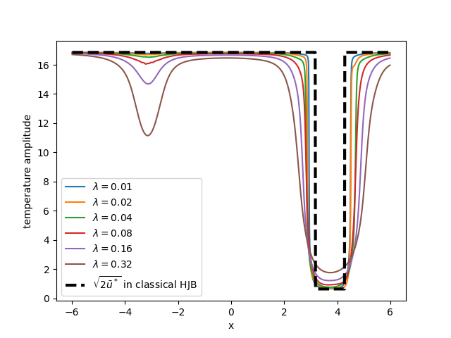
From Figure 2(b), we obtain that $v_{\lambda,\phi}^{\prime\prime}$ (from PINNs) closely matches the reference $v^{\prime\prime}$ for various $\lambda$’s. Moreover, $h_{\lambda,\phi}$ reproduces the qualitative shape of $\sqrt{2\bar{u}^{*}}$ and attains its minimum near the global minimizer $x=4$; see Figure 2(c).

(a) Objective $f$

(b) $v_{\lambda,\phi}^{\prime\prime}$ vs. $v^{\prime\prime}$

(c) $h_{\lambda,\phi}$ vs. $\sqrt{2\bar{u}^{*}}$

Figure 2: Example 5.2 (1D double-well). (a) Objective $f$. (b) $v_{\lambda,\phi}^{\prime\prime}$ for multiple $\lambda$ compared with the reference $v^{\prime\prime}$ (Appendix A). (c) $h_{\lambda,\phi}$ compared with $\sqrt{2\bar{u}^{*}}$ from (4).

In Algorithm 2, we take the step size $\eta=0.016$. In this example, $h_{\lambda,\phi}$ remains positive near $x=4$. Thus, without truncation ($\tau=0$ in (17)), the dynamics oscillates and the trajectory-averaged objective $\hat{f}_{k}$ exhibits sustained large fluctuations (Figure 3, left). With truncation $\tau=\tfrac{1}{2}\sqrt{2u_{\max}}$, the trajectory are stable and converge for all tested $\lambda$’s within $200$ iterations (Figure 3, right). Thus, accurate recovery of the shape of the curvature/noise coefficient is sufficient for the considered minimization problem and the truncation provides a simple mechanism for stable minimization.

Figure 3: 1D double-well: $\hat{f}_{k}$ (100-trajectory average) for multiple $\lambda$. Left: $\tau=0$. Right: $\tau=\tfrac{1}{2}\sqrt{2u_{\max}}$.

Example 5.3 (2D Gaussian mixture, [6]).

Let $\Omega=[-1,5]^{2}$. Consider the Gaussian-mixture objective

(22) $$f(\bm{x})=-\sum_{i=1}^{M}w_{i}\exp\left(-\frac{1}{2}\left(\bm{x}-\bm{m}_{i}\right)^{T}\Sigma_{i}^{-1}\left(\bm{x}-\bm{m}_{i}\right)\right),$$

where $M=25$ and $\{\bm{m}_{i}\}_{i=1}^{25}$ are placed on the grid $\{0,1,2,3,4\}^{2}$ (row-major order), the covariances are $\Sigma_{i}=0.1\,I_{2}$, and the mixture weights $\{w_{i}\}$ are listed in Table 5. In Figure 4, we plot the function and observe multiple wells and saddle regions; the deepest well is associated with the largest weight, where $\bm{x}_{*}=(3,2)$.

Table 5: Component means $\bm{m}_{i}$ and weights $w_{i}$ for Example 5.3 (row-major order on $\{0,1,2,3,4\}^{2}$).

$i$	$m_{i}$	$w_{i}$	$i$	$m_{i}$	$w_{i}$	$i$	$m_{i}$	$w_{i}$	$i$	$m_{i}$	$w_{i}$	$i$	$m_{i}$	$w_{i}$
1	(0,0)	0.4559	2	(0,1)	0.2559	3	(0,2)	0.3089	4	(0,3)	0.2974	5	(0,4)	0.2947
6	(1,0)	0.4972	7	(1,1)	0.5326	8	(1,2)	0.3268	9	(1,3)	0.4997	10	(1,4)	0.5220
11	(2,0)	0.4020	12	(2,1)	0.3167	13	(2,2)	0.5011	14	(2,3)	0.3068	15	(2,4)	0.4747
16	(3,0)	0.4392	17	(3,1)	0.5339	18	(3,2)	1.6552	19	(3,3)	0.4931	20	(3,4)	0.4037
21	(4,0)	0.3124	22	(4,1)	0.2915	23	(4,2)	0.3972	24	(4,3)	0.4242	25	(4,4)	0.2974

In this example, we study the effects of the control parameters $(u_{\min},u_{\max},\rho,\lambda)$ on the resulting Langevin dynamics. Specifically, we vary one of the control parameters at a time while freezing the rest. The goal is to identify which choices most affect convergence to the global minimizer to guide the choices in subsequent examples.

We set $N_{\partial\Omega}=128$ in (10) and obtain $\kappa=4.1$ from (15). In Algorithm 2, we use the step size $\eta=0.016$.

Figure 4: Example 5.3: 2D Gaussian mixture on $\Omega=[-1,5]^{2}$ (contour and surface). The landscape contains multiple wells; the deepest well is near $(3,2)$. Left: contour plot of $f$; right: surface plot.

We first test the effects of the control bounds $u_{\min}$ and $u_{\max}$. In Figure 5 (left), we plot the error $\mathcal{E}_{k}$ (over $N_{\mathrm{traj}}=100$ trajectories) versus the Langevin iteration index $k$, fixing $(\lambda,\rho,u_{\max},\tau)=(0.04,1.6,4\kappa,0)$ and varying $u_{\min}=10^{-8},10^{-6},10^{-4},10^{-2}$. In all tested cases, $\mathcal{E}_{k}\leq 0.1$ by $k=500$ and remains below this level thereafter. In Figure 5 (right), we vary $u_{\max}=\kappa\times 2^{p},p=-2,-1,0,1,2,3,4$, while fixing $(u_{\min},\lambda,\rho,\tau)=(10^{-8},0.04,1.6,0)$. The numerical results show that a larger $u_{\max}$ leads to faster convergence. Specifically, for $u_{\max}\geq\kappa$, we have $\mathcal{E}_{k}\leq 0.15$ by $k=500$ and continued improvement thereafter. When $u_{\max}=\kappa/2$, we observe $\mathcal{E}_{k}\approx 0.399$ by $k=500$ and about $0.132$ at the final iteration. When $u_{\max}=\kappa/4$, the error $\mathcal{E}_{k}$ remains large ($\mathcal{E}_{k}\approx 1.131$ by $k=500$ and about $0.662$ at the end). This figure suggests that choosing $u_{\max}\geq\kappa$ yields faster convergence while $u_{\min}$ should be kept close to zero.

Figure 5: Example 5.3: $\mathcal{E}_{k}$ (100-trajectory average). Left: varying $u_{\min}$ (curves nearly overlap). Right: varying $u_{\max}$ (larger $u_{\max}$ yields faster convergence).

Next, we test the effects of $\lambda$ . In Figure 6 (left), we plot $\mathcal{E}_{k}$ versus the Langevin iteration index $k$, fixing $(u_{\min},\rho,u_{\max},\tau)=(10^{-8},1.6,4\kappa,0)$ and varying $\lambda=0.01\times 2^{p}$, $p=0,1,\ldots,5$. For $\lambda=0.01,0.02,0.04$, the trajectories enter the $0.1$-neighborhood of the global minima by $k=500$ and remain in the region. For $\lambda=0.08,0.16$, the error $\mathcal{E}_{k}$ is larger (about $0.1$–$0.2$ at $k=500$), while for $\lambda=0.32$ the trajectories remain far from the minimizer set (with $\mathcal{E}_{k}$ oscillating around $1.8$).

Moreover, introducing truncation as in (17) improves the accuracy in the error $\mathcal{E}_{k}$, for large $\lambda$. Fixing $(u_{\min},u_{\max},\rho,\lambda)=(10^{-8},4\kappa,1.6,0.32)$ and take $\tau=s\sqrt{2u_{\max}},\;s=0,\frac{1}{8},\frac{1}{4},\frac{1}{2}$. For $\tau=s\sqrt{2u_{\max}},\;s=\frac{1}{4},\frac{1}{2}$, we observe that $\mathcal{E}_{k}<10^{-4}$ by $k=800$; see Figure 6 (middle).

Third, we vary the discount rate $\rho$. Specifically, we take $\rho=0.2\times 2^{p},p=1,2,...8$. and fix $(u_{\min},\lambda,u_{\max},\tau)=(10^{-8},0.04,4\kappa,0)$. We observe from Figure 6 (right) that moderately large $\rho$’s lead to fast convergence: for $\rho=0.2,0.4,0.8,1.6,3.2$, we obtain $\mathcal{E}_{k}\leq 0.15$ by $k=500$; whereas larger $\rho$ yields slow convergence within a small number of iterations.

Figure 6: Example 5.3: $\mathcal{E}_{k}$ (100-trajectory average). Left: varying $\lambda$. Middle: varying $\tau$ with $(u_{\max},u_{\min},\lambda)=(4\kappa,10^{-8},0.32)$. Right: varying $\rho$. Smaller $\lambda$ and truncation for large $\lambda$ improve convergence; larger $\rho$ mainly slows early iterations.

In summary, the numerical results suggest that satisfactory performance of the stochastic Langevin dynamics for the minimization problem depends more on $u_{\max}$ (no smaller than $\kappa$) and the regularization rate $\lambda$ than on $u_{\min}$ and the discount rate $\rho$. Also, truncation in the noise coefficients (17) improves convergence for large $\lambda$ and both small and large $\rho$’s work well, but large $\rho$’s tend to slow down the convergence in early iterations.

In the following examples, we will follow the observations from Example 5.3 to set $(u_{\min},u_{\max},\rho,\lambda)$. Moreover, we only vary the truncation level $\tau$ to illustrate its practical role in stabilizing the trajectories. We present additional simulations with various $\lambda$’s in Appendix B.

Example 5.4 (Easom function, minima in a plateau).

Let $\Omega=[-10,10]^{2}$ and

$$f(\bm{x})=-\cos(x_{1})\cos(x_{2})\exp\!\bigl(-(x_{1}-\pi)^{2}-(x_{2}-\pi)^{2}\bigr),\qquad\bm{x}=(x_{1},x_{2})\in\Omega.$$

The landscape is nearly flat around the unique global minimizer at $\bm{x}^{*}=(\pi,\pi)$.

In this example, we choose $N_{\partial\Omega}=4096$ in (10) and compute $\kappa=0.56$ in (15). In Algorithm 2, we use the step size $\eta=0.128$. We set $(u_{\min},u_{\max},\rho,\lambda)=(10^{-8},16\kappa,0.2,0.01)$.

We plot in Figure 7 (left) the errors of numerical global minimizers $\mathcal{E}_{k}$ versus the Langevin iteration index $k$ for several truncation levels $\tau$. We observe that larger truncation improves terminal accuracy: $\tau=s\sqrt{2u_{\max}},\,s=\frac{1}{8},\frac{1}{4},\frac{1}{2}$ yields the smaller terminal $\mathcal{E}_{k}$ (near zero), whereas smaller $\tau=0,\frac{1}{16}\sqrt{2u_{\max}}$ give errors $\mathcal{E}_{k}$’s. The numerical results in this example show that the proposed PINN-based temperature from the eHJB equations can help find a global minimizer of non-convex functions with plateau landscapes.

Example 5.5 (Hartmann 6D function).

Consider the Hartmann function

$$f(\bm{x})=\frac{1}{1.94}\Bigl(-\sum_{i=1}^{4}\alpha_{i}\exp\!\Bigl(-\sum_{j=1}^{6}A_{ij}(x_{j}-P_{ij})^{2}\Bigr)+2.58\Bigr),\quad\bm{x}\in\Omega=[0,1]^{6},$$

with $\alpha=(1.0,1.2,3.0,3.2)^{\top}$ and $A,\,P\in\mathbb{R}^{4\times 6}$ given below:

$$\mathbf{A}=\begin{bmatrix}10&3&17&3.50&1.7&8\\ 0.05&10&17&0.1&8&14\\ 3&3.5&1.7&10&17&8\\ 17&8&0.05&10&0.1&14\end{bmatrix},\quad\mathbf{P}=10^{-4}\begin{bmatrix}1312&1696&5569&124&8283&5886\\ 2329&4135&8307&3736&1004&9991\\ 2348&1451&3522&2883&3047&6650\\ 4047&8828&8732&5743&1091&381\end{bmatrix}.$$

This function is multimodal with multiple local minima; the global minimizer is $\bm{x}_{*}=(0.20169,0.150011,0.476874,0.275332,0.311652,0.6573)$ and $f(\bm{x}_{*})=-3.32237$.

We set $N_{\partial\Omega}=4096$ in (10) and obtain $\kappa=16$ from (15). In Algorithm 2, we take the step size $\eta=0.016$. Set $(u_{\min},u_{\max},\rho,\lambda)=(10^{-8},\kappa,1.6,0.02)$.

We plot in Figure 7 (right) the errors of numerical global minimizers $\mathcal{E}_{k}$ versus the Langevin iteration index $k$, for $\tau=s\sqrt{2u_{\max}},s=0,\tfrac{1}{16},\tfrac{1}{8},\tfrac{1}{4},\tfrac{1}{2}$. we observe that $\tau=\tfrac{1}{16}\sqrt{2u_{\max}}$ yields the best performance, while larger truncation levels increase the error $\mathcal{E}_{k}$ when $k$ is large. For comparison, with $\tau=0$ we observe a plateau at $\mathcal{E}_{k}\approx 0.075$ for $k\geq 200$, whereas $s=\tfrac{1}{16}$ yields smaller $\mathcal{E}_{k}$ at later iterations. The results suggest that a moderate truncation is preferred for this 6D multimodal benchmark.

Figure 7: Left: Example 5.4 (Easom), $\mathcal{E}_{k}$ for $\tau=\sqrt{2u_{\max}},s=0,\tfrac{1}{16},\tfrac{1}{8},\tfrac{1}{4},\tfrac{1}{2}$. Right: Example 5.5 (Hartmann-6), $\mathcal{E}_{k}$ for the same truncation set.

6 Conclusion and discussion

The minimization problems solved with Langenvin dynamics were studied via controlled diffusions and the corresponding exploratory HJB equation. We apply physics-informed neural networks to solve the exploratory HJB equation. The quantity of most interest, the trace of the Hessian, is proved to converge with order one in the regularization parameter $\lambda$. Further analysis shows that the error induced by the physics-informed neural networks is at the order of the magnitude of PDE residual (Theorem 4.1). We demonstrate through several representative examples that the approach can be effective for solving minimization problems up to 6 dimensions, including overcoming saddle points and finding a global minimum on a plateau. However, the computational cost is high due to the PINN solvers for eHJB equations. Further computational cost reduction may come from using the solution structure of eHJB equations as well as more advanced techniques, such as tensor neural networks (e.g. [31]) and random mini-batch in dimensionality [15]. Also, systematic studies on classical optimization benchmark functions should be conducted.

Appendix A Monotone finite differences and Howard policy iteration for the classical HJB equation

We briefly summarize the numerical scheme used to compute the PDE-based reference solution of the classical HJB equation (3) on $\Omega=(x_{L},x_{R})$ with homogeneous Neumann boundary conditions

(23) $$v_{x}(x_{L})=0,\qquad v_{x}(x_{R})=0.$$

Denote $b(\bm{x}):=-f^{\prime}(\bm{x})$ for simplicity. We use a uniform grid $x_{i}=x_{L}+i\Delta x$ for $i=0,\dots,N-1$ with $\Delta x=(x_{R}-x_{L})/(N-1)$ and unknowns $v_{i}\approx v(x_{i})$. The Neumann conditions (23) are enforced by

(24) $$\frac{v_{1}-v_{0}}{\Delta x}=0,\qquad\frac{v_{N-1}-v_{N-2}}{\Delta x}=0.$$

At interior nodes $i=1,\dots,N-2$, we discretize $v_{xx}$ by a central difference and $b\,v_{x}$ by an upwind difference:

$$v_{xx}(x_{i})\approx\frac{v_{i+1}-2v_{i}+v_{i-1}}{(\Delta x)^{2}},\qquad b(x_{i})v_{x}(x_{i})\approx b_{i}^{+}\frac{v_{i}-v_{i-1}}{\Delta x}+b_{i}^{-}\frac{v_{i+1}-v_{i}}{\Delta x},$$

where $b_{i}=b(x_{i})$, $b_{i}^{+}=\max(b_{i},0)$, and $b_{i}^{-}=\min(b_{i},0)$. For a fixed grid control $u_{i}\in[u_{\min},u_{\max}]$, the resulting interior equation is

(25) $$-\rho v_{i}+f_{i}+u_{i}\frac{v_{i+1}-2v_{i}+v_{i-1}}{(\Delta x)^{2}}+b_{i}^{+}\frac{v_{i}-v_{i-1}}{\Delta x}+b_{i}^{-}\frac{v_{i+1}-v_{i}}{\Delta x}=0,\,i=1,\dots,N-2.$$

We solve the resulting nonlinear system using Howard’s policy iteration.

In Example 5.2, $\Omega=[x_{L},x_{R}]=[-6,6]$ and we use a uniform grid with $N=1001$ points (spacing $\Delta x=(x_{R}-x_{L})/(N-1)$), discount rate $\rho=0.4$, and diffusion control $u(\bm{x})\in[u_{\min},u_{\max}]=[0.2,142]$; Howard iteration is run in double precision and stops when $\|u^{(k+1)}-u^{(k)}\|_{\infty}<\varepsilon_{u}=10^{-4}$ or when $k$ reaches $k_{\max}=2000$.

Appendix B Additional tests for Easom and Hartmann-6

We present in Figure  8 additional tests with several $\lambda$’s for the Easom and Hartmann-6 optimization problems under fixed $(u_{\min},u_{\max},\rho,\tau)$ and step size $\eta$. We observe that small errors $\mathcal{E}_{k}$, $k\leq 1000$, of the numerical global minimizers for $\lambda=0.01,0.02,0.04,0.08,0.16$. However, a relatively small $\lambda$ is preferred in simulations.

(a) Easom: varying $\lambda$

(b) Hartmann-6: varying $\lambda$

Figure 8: Additional tests of the errors $\mathcal{E}_{k}$ of numerical global minimizers with various $\lambda$’s. (a) Easom with $(u_{\min},u_{\max},\rho,\tau)=(10^{-8},16\kappa,0.02,0)$ and step size $\eta=0.128$. (b) Hartmann-6 with $(u_{\min},u_{\max},\rho,\tau)=(10^{-8},\kappa,1.6,0.02)$ and step size $\eta=0.016$. In both cases, $\lambda=0.01,0.02,0.04,0.08,0.16$.

Appendix C Proofs

From Theorem 4.1, $\Omega$ is open and bounded with a smooth boundary. Then we obtain that $v,v_{\lambda}\in C^{2,\alpha}$ with $\alpha\in(0,1)$ depends on dimension $d$ and $u_{\min}>0$. Define $H_{\lambda}(\bm{x})=-\lambda\ln\int_{u_{\min}}^{u_{\max}}\exp\left(-{\lambda}^{-1}{\operatorname{Tr}X}u\right)du$, and $H(\bm{x})=(u_{\min}\chi_{\operatorname{Tr}X>0}+u_{\max}\chi_{\operatorname{Tr}X<0})\operatorname{Tr}X$, where $\chi_{A}(\cdot)$ is the indicator function on the set $A$.

By direct calculations (or see Lemma 4.4 of [29]), we have, for any $X,Y\in\mathbb{R}^{d\times d}$,

(26) $$u_{\min}\|X-Y\|\leq\left|H(\bm{x})-H(Y)\right|\leq u_{\max}\|X-Y\|.$$

Lemma C.1.

Suppose that $X\in C^{0,\alpha}$, $\alpha\in(0,1)$. There exists $C>0$ independent of $\lambda$ such that

$$\|H_{\lambda}(\bm{x})-H(\bm{x})\|_{C^{0,\gamma}}\leq C\lambda^{1-\gamma/\alpha},\,0\leq\gamma<\alpha.$$

Proof.

Let $Y=X(y)$ and $X=X(\bm{x})$, $x,y\in\Omega$. By direct calculations, $\left|\left|DH_{\lambda}\right|\right|\leq C$ and $\left|\left|D^{2}H_{\lambda}\right|\right|\leq C\lambda^{-1}$, where $C$ is independent of $\lambda$. The conclusion for $\gamma=0$ then follows from the Lipschitz continuity of $H$ and $H_{\lambda}$ and direct calculations.

By Taylor’s formula on $H_{\lambda}(\bm{x})$ around $Y$, we have

$$\left|H_{\lambda}(\bm{x})-H(\bm{x})-\big({H_{\lambda}(Y)-H(Y)}\big)\right|$$

$$\leq\left|H(\bm{x})-H(Y)\right|+\left|H_{\lambda}(\bm{x})-H_{\lambda}(Y)\right|$$

$$\leq C\left|\left|X-Y\right|\right|+\left|DH_{\lambda}:(X-Y)\right|+C\left|\left|D^{2}H_{\lambda}\right|\right|\left|\left|X-Y\right|\right|^{2}$$

$$\leq C\left|\left|X-Y\right|\right|+C\lambda^{-1}\left|\left|X-Y\right|\right|^{2},$$

where the constant $C$ may change from step to step, while remaining a constant (the same applies to the rest of the argument). Since both $X$ and $Y$ are in $C^{0,\alpha}$, we have, for $0<\gamma<\alpha$,

$$\frac{\left|H_{\lambda}(\bm{x})-H(\bm{x})-\big({H_{\lambda}(Y)-H(Y)}\big)\right|}{\left|x-y\right|^{\gamma}}\leq C\left|x-y\right|^{\alpha-\gamma}+C\lambda^{-1}\left|x-y\right|^{2\alpha-\gamma}.$$

It can be readily verified that when $\left|x-y\right|^{\alpha}$ is at the order of $\lambda$, the right-hand side will reach its supremum, which is at the order of $\lambda^{1-\gamma/\alpha}$.

Theorem C.2.

Suppose that $f\in C^{2}(\Omega)$. Then

(27) $$\sqrt{u_{\min}}\left|\left|\nabla v_{\lambda}-\nabla v\right|\right|_{L^{\infty}(\Omega)}+u_{\min}\left|\left|\Delta v_{\lambda}-\Delta v\right|\right|_{L^{\infty}(\Omega)}\leq C\big(\left|\left|w_{\lambda}\right|\right|_{L^{\infty}(\Omega)}+\left|\left|g_{\lambda}\right|\right|_{L^{\infty}(\Omega)}\big)\leq C\lambda.$$

Proof of Theorem C.2.

The difference $w_{\lambda}=v_{\lambda}-v$ satisfies the following equation

(28) $$\rho w_{\lambda}-\nabla f\cdot\nabla w_{\lambda}+A_{\lambda}\Delta w_{\lambda} =H(D^{2}v)-H_{\lambda}(D^{2}v)=:g_{\lambda}(\bm{x})$$

where we apply Taylor’s theorem $H_{\lambda}(D^{2}v_{\lambda})-H_{\lambda}(D^{2}v)=A_{\lambda}(\Delta v_{\lambda}-\Delta v)$ and $A_{\lambda}=\int_{0}^{1}DH_{\lambda}\left(D^{2}v+s(D^{2}v_{\lambda}-D^{2}v)\right)\,ds$.

Since $u_{\min}I\leq A_{\lambda}$, the equation of $w_{\lambda}$ is uniformly elliptic. By the equation (28) and $f\in C^{2}$, we have

(29) $$u_{\min}\left|\left|\Delta w_{\lambda}\right|\right|_{L^{\infty}(\Omega)}\leq C_{K}\big(\left|\left|w_{\lambda}\right|\right|_{L^{\infty}(\Omega)}+\left|\left|\nabla w_{\lambda}\right|\right|_{L^{\infty}(\Omega)}+\left|\left|g_{\lambda}\right|\right|_{L^{\infty}(\Omega)}\big),$$

and by the interpolation inequality $\left|\left|\nabla w_{\lambda}\right|\right|_{L^{\infty}(\Omega)}\leq C_{K}\left|\left|w_{\lambda}\right|\right|_{L^{\infty}(\Omega)}^{1/2}\left|\left|\Delta w_{\lambda}\right|\right|_{L^{\infty}(\Omega)}^{1/2}$, we obtain that

$$u_{\min}\left|\left|\Delta w_{\lambda}\right|\right|_{L^{\infty}(\Omega)}\leq C\big(\left|\left|w_{\lambda}\right|\right|_{L^{\infty}(\Omega)}+\left|\left|g_{\lambda}\right|\right|_{L^{\infty}(\Omega)}\big).$$

Then by Lemma C.1 and $\left|\left|w_{\lambda}\right|\right|_{L^{\infty}(\Omega)}\leq C\lambda$ ([29]), ${u_{\min}}\left|\left|\Delta w_{\lambda}\right|\right|_{L^{\infty}(\Omega)}\leq C\lambda$. Then, by the interpolation inequality above, $\sqrt{u_{\min}}\left|\left|\nabla w_{\lambda}\right|\right|_{L^{\infty}(\Omega)}\leq C\lambda$ and thus (27) holds.

Theorem C.3.

Suppose that $f\in C^{2}(\Omega)$ and $\widetilde{R}_{\lambda}(\bm{x},\phi)\in L^{\infty}(\Omega)$ in (11). Then we have

$$\sqrt{u_{\min}}\left|\left|\nabla(v_{\lambda}-v_{\lambda,\phi})\right|\right|_{L^{\infty}(\Omega)}+u_{\min}\left|\left|\Delta(v_{\lambda}-v_{\lambda,\phi})\right|\right|_{L^{\infty}(\Omega)} \leq C\varepsilon\left|\left|\widetilde{R}_{\lambda}(\cdot,\phi)\right|\right|_{L^{\infty}},\,\varepsilon>0.$$

The proof is similar to that of Theorem C.3 and thus omitted. The only difference lies in the fact that (11) is not an actual equation and is rather a value of the eHJB operator evaluated at $v_{\lambda,\phi}$.

References

- [1] A. Arakelyan and R. Barkhudaryan, Convergence of physics-informed neural networks for fully nonlinear pde’s, arXiv:2501.04013, (2024).
- [2] R. Bertrand and R. Epenoy, New smoothing techniques for solving bang-bang optimal control problems—numerical results and statistical interpretation, Optimal Control Appl. Methods, 23 (2002), pp. 171–197.
- [3] O. Bokanowski, S. Maroso, and H. Zidani, Some convergence results for Howard’s algorithm, SIAM J. Numer. Anal., 47 (2009), pp. 3001–3026.
- [4] X. Chen, C. Liang, D. Huang, E. Real, K. Wang, Y. Liu, H. Pham, X. Dong, T. Luong, C.-J. Hsieh, Y. Lu, and Q. V. Le, Symbolic Discovery of Optimization Algorithms, arXiv e-prints, (2023), p. arXiv:2302.06675.
- [5] M. G. Crandall, H. Ishii, and P.-L. Lions, User’s guide to viscosity solutions of second order partial differential equations, Bull. Amer. Math. Soc. (N.S.), 27 (1992), pp. 1–67.
- [6] J. Dong and X. T. Tong, Replica exchange for non-convex optimization, J. Mach. Learn. Res., 22 (2021), pp. Paper No. 173, 59.
- [7] J.-L. Dupret and D. Hainaut, Deep learning for high-dimensional continuous-time stochastic optimal control without explicit solution, Operations Research, (2026).
- [8] M. Falcone and R. Ferretti, Semi-Lagrangian approximation schemes for linear and Hamilton-Jacobi equations, Society for Industrial and Applied Mathematics (SIAM), Philadelphia, PA, 2014.
- [9] X. Feng, T. Lewis, and A. Rapp, Dual-wind discontinuous Galerkin methods for stationary Hamilton-Jacobi equations and regularized Hamilton-Jacobi equations, Commun. Appl. Math. Comput., 4 (2022), pp. 563–596.
- [10] W. H. Fleming and H. M. Soner, Controlled Markov processes and viscosity solutions, vol. 25 of Applications of Mathematics (New York), Springer-Verlag, New York, 1993.
- [11] X. Gao, Z. Q. Xu, and X. Y. Zhou, State-dependent temperature control for Langevin diffusions, SIAM J. Control Optim., 60 (2022), pp. 1250–1268.
- [12] S. Geman and C.-R. Hwang, Diffusions for global optimization, SIAM J. Control Optim., 24 (1986), pp. 1031–1043.
- [13] B. Hajek, Cooling schedules for optimal annealing, Math. Oper. Res., 13 (1988), pp. 311–329.
- [14] J. Han, A. Jentzen, and W. E, Solving high-dimensional partial differential equations using deep learning, Proc. Natl. Acad. Sci. USA, 115 (2018), pp. 8505–8510.
- [15] Z. Hu, K. Shukla, G. E. Karniadakis, and K. Kawaguchi, Tackling the curse of dimensionality with physics-informed neural networks, Neural Networks, 176 (2024), p. 106369.
- [16] Z. Hu, Z. Zhang, G. E. Karniadakis, and K. Kawaguchi, Score-based physics-informed neural networks for high-dimensional Fokker-Planck equations, SIAM J. Sci. Comput., 47 (2025), pp. C680–C705.
- [17] Y. Huang, P. A. Forsyth, and G. Labahn, Combined fixed point and policy iteration for Hamilton-Jacobi-Bellman equations in finance, SIAM J. Numer. Anal., 50 (2012), pp. 1861–1882.
- [18] C. Huré, H. Pham, and X. Warin, Deep backward schemes for high-dimensional nonlinear PDEs, Math. Comp., 89 (2020), pp. 1547–1579.
- [19] Y. Kim, N. Cho, M. Kim, and Y. Kim, Physics-informed approach for exploratory Hamilton–Jacobi–Bellman equations via policy iterations, arXiv:2508.01720, (2025).
- [20] T. Liu, S. Ding, J. Zhang, and L. Zhou, Pinn-based viscosity solution of HJB equation, arXiv:2309.09953, (2023).
- [21] Y. Meng, R. Zhou, A. Mukherjee, M. Fitzsimmons, C. Song, and J. Liu, Physics-informed neural network policy iteration: Algorithms, convergence, and verification, arXiv:2402.10119, (2024).
- [22] T. Munakata and Y. Nakamura, Temperature control for simulated annealing, Phys. Rev. E, 64 (2001), p. 046127.
- [23] T. Nakamura-Zimmerer, Q. Gong, and W. Kang, Adaptive deep learning for high-dimensional Hamilton-Jacobi-Bellman equations, SIAM J. Sci. Comput., 43 (2021), pp. A1221–A1247.
- [24] A. Neelakantan, L. Vilnis, Q. V. Le, I. Sutskever, L. Kaiser, K. Kurach, and J. Martens, Adding gradient noise improves learning for very deep networks, arXiv:1511.06807, (2015).
- [25] M. Raginsky, A. Rakhlin, and M. Telgarsky, Non-convex learning via stochastic gradient Langevin dynamics: a nonasymptotic analysis, in Proceedings of the 2017 Conference on Learning Theory, PMLR, 2017, pp. 1674–1703.
- [26] M. Raissi, P. Perdikaris, and G. Karniadakis, Physics-informed neural networks: A deep learning framework for solving forward and inverse problems involving nonlinear partial differential equations, Journal of Computational Physics, 378 (2019), pp. 686–707.
- [27] C. Silva and E. Trélat, Smooth regularization of bang-bang optimal control problems, IEEE Transactions on Automatic Control, 55 (2010), pp. 2488–2499.
- [28] J. Sirignano and K. Spiliopoulos, Dgm: A deep learning algorithm for solving partial differential equations, Journal of Computational Physics, 375 (2018), pp. 1339–1364.
- [29] W. Tang, Y. P. Zhang, and X. Y. Zhou, Exploratory HJB equations and their convergence, SIAM J. Control Optim., 60 (2022), pp. 3191–3216.
- [30] H. Wang, T. Zariphopoulou, and X. Y. Zhou, Reinforcement learning in continuous time and space: A stochastic control approach, Journal of Machine Learning Research, 21 (2020), pp. 1–34.
- [31] T. Wang, Z. Hu, K. Kawaguchi, Z. Zhang, and G. E. Karniadakis, Tensor neural networks for high-dimensional fokker–planck equations, Neural Networks, 185 (2025), p. 107165.
- [32] P. Xu, J. Chen, D. Zou, and Q. Gu, Global convergence of Langevin dynamics based algorithms for nonconvex optimization, in Advances in Neural Information Processing Systems, S. Bengio, H. Wallach, H. Larochelle, K. Grauman, N. Cesa-Bianchi, and R. Garnett, eds., vol. 31, Curran Associates, Inc., 2018.
- [33] M. Zhou, J. Han, and J. Lu, Actor-critic method for high dimensional static Hamilton-Jacobi-Bellman partial differential equations based on neural networks, SIAM J. Sci. Comput., 43 (2021), pp. A4043–A4066.