Optimal transport of an active particle near a plane wall

Abstract

The control of active colloidal particles via optical traps is a cornerstone for research of matter at the micron and nanometer scale. A central challenge in this domain is the derivation of optimal transport protocols that minimize the mean work required to move a particle over a finite-time interval. Here we present a Ritz method in which open-loop protocols are constructed from a global basis of Chebyshev polynomials and optimised by a genetic algorithm. We apply the method to study optimal transport of an active particle, which is modelled as a force-dipole (or a stresslet) near a no-slip wall. The methodology is validated in the limits of zero activity and infinite wall separation, where it successfully recovers the known analytical protocols and the theoretical minimum work. Crucially, we demonstrate that the presence of the boundary breaks the time-reversal symmetry of the optimal protocol found in bulk solutions. This symmetry breaking is shown to be a complex function of the transport direction and the particle’s intrinsic activity. Because the presented approach requires only the capability to simulate stochastic trajectories, it offers a robust, principled framework for optimizing transport protocols in complex fluid environments that remain inaccessible to exact analytical treatment.

I Introduction

The minimization of thermodynamic work during the finite-time transport of colloidal particles is a canonical problem in stochastic thermodynamics [1, 2, 3]. Optical tweezers provide a natural means of confining and transporting such particles [4], and the question of how to do so efficiently is both practically relevant and theoretically rich. In a bulk fluid environment, the analytical solution was derived in a seminal paper by Schmiedl and Seifert [5], which established that the optimal transport protocol for a passive Brownian particle in a translating harmonic trap is a linear ramp bounded by jump discontinuities. Active colloidal particles, which dissipate energy from their environment to create mechanical disturbance around them, have attracted sustained interest as model systems for nonequilibrium physics [6, 7, 8]. Deriving protocols for the transport of active colloidal particles is topic of recent investigations using theory and experiments [9, 10, 11, 12, 13, 14, 15, 16, 17]. Current studies focus on particles in bulk fluid, while in many practical and experimental settings particles are frequently confined and transported in the vicinity of solid boundaries.

Near a solid boundary, the thermodynamic work done in transporting active particles is modified by two distinct hydrodynamic phenomena that are absent in the bulk. First, the spatially dependent friction suppresses the particle’s diffusion as it approaches the wall. Second, the motion of the active particle is modified due to hydrodynamic interactions with the no-slip boundary. When modeled as a stresslet (a force dipole) [18, 19], an active particle generates a flow field that is modified near the wall via the Blake image system [20]. Crucially, the resulting wall-induced drift is highly direction-dependent: extensile swimmers ("pushers") are hydrodynamically repelled from the boundary, whereas contractile swimmers ("pullers") are attracted.

In this paper, we demonstrate how the interplay of spatially dependent mobility and asymmetric active drift fundamentally modifies the stochastic thermodynamics of near-wall transport of active particles. We show that the boundary-induced effects profoundly distort the minimum-work optimal control protocols. To this end, we note that the coupling between the spatially varying Brenner friction and the wall-induced active drift introduces severe nonlinearities into the governing equations, rendering exact analytical solutions for the minimum-work protocols intractable.

A variety of numerical methods have been developed for optimising time-dependent protocols in stochastic systems, including Monte Carlo schemes, genetic algorithm, and gradient-based algorithms [21, 22, 23]. Genetic algorithms (GAs) are particularly well suited to problems of this kind: they require only the ability to evaluate the objective function, are robust to noise, and impose no smoothness requirements on the protocol ansatz [22, 23]. In this paper, we use GA, while the protocol is represented in a Ritz basis, which provides a compact and flexible ansatz that naturally accommodates the jump discontinuities known to appear at the endpoints of optimal protocols [5, 9]. Thus, our method is distinct from [22, 23], where parameters of a deep learning model were obtained using GA. Our GA implementation is validated against the Schmiedl–Seifert exact solution [5], and then applied across a systematic grid of initial wall separations $H_{0}$ and dimensionless activity parameter $\alpha$, for both away-from-wall and towards-wall protocols.

The rest of the paper is organised as follows. Section II describes the physical model, including the Brenner mobility and the stresslet active drift. This section also describes the Ritz method, Chebyshev polynomials for protocol representation, and the genetic algorithm. Section III presents the results of the paper. Section IV summarises the findings and suggests directions for future work.

II Model and Methodology

II.1 System setup

A spherical active colloidal particle of radius $b$ is immersed in a Newtonian fluid of viscosity $\eta$ at temperature $T$ at height $h$ above an infinite planar no-slip wall (Fig. 1). The particle is confined in a harmonic optical trap of stiffness $k$ whose centre $\lambda(t)$ is the control parameter. The task is to move $\lambda$ from $\lambda_{i}=H_{0}b$ to $\lambda_{f}=(H_{0}+\Delta H)b$ in a fixed time $t_{f}$ while minimising the mean thermodynamic work. We restrict attention to the wall-normal direction $h$, which captures the dominant physics of wall-proximity effects.

II.2 Equation of motion

We now consider the stochastic motion of an active colloidal particle. The dynamics of the active colloidal particle, which is confined in a harmonic potential (see Fig. 1), is given according to the overdamped Langevin equation [24]:

$$\dot{h} =-\mu(h)\,\partial_{h}V(h,\lambda(t))+v^{\mathcal{A}}(h)+\sqrt{2D(h)}\,\xi(t)$$ (1a)

$$=A(h)+\sqrt{B(h)}\,\xi(t)$$ (1b)

Here, $\mu(h)$ is the spatially dependent mobility and $D(h)=\mu(h)k_{B}T$ is the local diffusion coefficient from the Einstein relation, with $k_{B}$ as the Boltzmann constant [25]. The stochastic variable $\xi(t)$ has zero mean $\langle\xi(t)\rangle=0$ and no temporal correlation $\langle\xi(t)\xi(t^{\prime})\rangle=\delta(t-t^{\prime})$. Thus, it is referred to as a ‘white’ noise. We note that $D(h)$ inherits the spatial dependence of $\mu(h)$; both the drift and the noise amplitude are therefore position-dependent, and this must be accounted for in the numerical integrator (see section II.5).

The bulk Stokes mobility of a sphere of radius $b$ in a fluid of viscosity $\eta$ is $\mu_{0}=1/(6\pi\eta b)$. Near a no-slip wall, the backflow generated by the wall image system reduces this value. For a particle near a solid wall, the mobility $\mu(h)$ follows from the Brenner formula [26]:

$$\mu(h)=\mu_{0}\left[1-\frac{9}{8}\frac{b}{h}+\frac{1}{8}\left(\frac{b}{h}\right)^{3}\right]$$ (2)

where $b$ is the particle radius. Proximity to the wall induces a deterministic active velocity [27]:

$$v^{\mathcal{A}}(h)=-\frac{s_{0}}{8}\left[\left(\frac{b}{h}\right)^{2}-\left(\frac{b}{h}\right)^{4}\right]$$ (3)

For a puller ($s_{0}>0$) the drift is directed towards the wall; for a pusher ($s_{0}<0$) it is directed away from the wall (see Fig. 9 in appendix C). Both the Brenner correction and the active drift vanish as $b/h\to 0$, recovering homogeneous bulk dynamics far from the wall.

II.3 Work done in moving a trapped particle

Consider a particle in a harmonic trap with a moving center $\lambda(t)$ and stiffness $k$:

$$V(h,\tau)=\frac{k}{2}(h-\lambda(\tau))^{2}$$ (4)

The mean thermodynamic work $\langle W\rangle$ performed during a time interval $[0,t_{f}]$ is defined as [28, 1, 2, 3]:

$$\langle W\rangle =\int_{0}^{t_{f}}dt\dot{\lambda}(t)\left\langle\frac{\partial V(h,\lambda(t))}{\partial\lambda}\right\rangle$$

$$=-k\int_{0}^{t_{f}}dt\dot{\lambda}(t)(\langle h(t)\rangle-\lambda(t))$$ (5)

In complex scenarios involving surface interactions or persistence, an analytical solution for the optimal protocol $\lambda^{*}(t)$ is generally unavailable; the numerical approach described in Section II.5 is therefore required.

Figure 1: Schematic of the system. An active colloidal particle (orange circle) is driven by a time-varying harmonic potential $V(\lambda(t))$. The particle exchanges energy with the trap, dissipates heat to the thermal bath, and self-generates drift through internal activity.

II.4 Ritz Method for Protocol Representation

In this section, we present the protocol representation for the Ritz method [29, 30]. The open-loop protocol is written as an expansion in Chebyshev polynomials $T_{n}$ [31]:

$$\lambda(t)=\sum_{n=0}^{N-1}a_{n}\,T_{n}\!\left(\frac{2t}{t_{f}}-1\right).$$ (6)

The boundary conditions $\lambda(0)=\lambda_{i}$ and $\lambda(t_{f})=\lambda_{f}$ are enforced exactly; the genetic algorithm optimises the coefficients $\{a_{n}\}$ to minimise $\langle W\rangle$. Chebyshev polynomials are a natural basis for this problem: they impose no smoothness constraint at the endpoints, so the jump discontinuities of Eq. (11) emerge naturally from the optimisation rather than being imposed a priori. This global spectral representation reduces the functional minimization to a multivariate optimization over a compact, discrete set of coefficients. In the implementation, the boundary conditions are enforced by appending the fixed endpoint values $\lambda_{i}$ and $\lambda_{f}$ directly to the protocol tensor before every physics evaluation, rather than as constraints on the coefficients themselves; the Chebyshev expansion thus parametrises strictly the interior of the time domain ($0<t<t_{f}$), and the jump discontinuities known to appear at $t=0^{+}$ and $t=t_{f}^{-}$ in optimal protocols emerge naturally.

The infinite series of Eq.6 is truncated at $N=5$ basis functions. Extensive preliminary sweeps over the range $N\in\{2,\dots,8\}$ revealed that the mean thermodynamic work plateaus for $N\geq 3$. We selected $N=5$ because it optimally minimizes the work relative to analytical bulk solutions; expanding the basis size further strains the fixed generation budget of the genetic algorithm without yielding additional thermodynamic savings. Thus, the genetic algorithm operates entirely within a 5-dimensional search space, optimizing the finite set of coefficients $\{a_{n}\}$ to minimize $\langle W\rangle$.

II.5 Genetic Algorithm

A population of $P=150$ individuals is initialised from a Gaussian distribution, with the zeroth Chebyshev coefficient biased toward the midpoint $H_{0}+\Delta H/2$ to seed plausible initial protocols. Each individual encodes a full protocol via basis evaluation at each timestep. Each protocol is evaluated by running $N_{\text{traj}}$ independent stochastic trajectories and computing $\langle W\rangle$ as the fitness to be minimised. Trajectories are integrated with the predictor–corrector (Heun) scheme

$$\tilde{h}^{(n+1)} =h^{(n)}+\Delta t\,A(h^{(n)})+\sqrt{B(h^{(n)})}\,dw^{(n)}$$ (7)

$$h^{(n+1)} =h^{(n)}+\frac{\Delta t}{2}\left[A(h^{(n)})+A(\tilde{h}^{(n+1)})\right]$$

$$\quad+\frac{1}{2}\left[\sqrt{B(h^{(n)})}+\sqrt{B(\tilde{h}^{(n+1)})}\right]\,dw^{(n)}$$

where $\alpha(h)$ is the total deterministic drift, while $B(h)=2D(h)$, and $dw^{(n)}$ is the Wiener increment (Gaussian noise) [32]. The timestep is $\Delta t=0.002$ with $N_{\text{steps}}=1000$ steps per trajectory over $t_{f}=2.0$. All trajectory evaluations are vectorised on a GPU using PyTorch [33].

Figure 2: Flowchart of the genetic algorithm. Each generation evaluates $\langle W\rangle$ via stochastic trajectory simulation, retains the top elites, and produces the next generation by tournament selection and annealed Gaussian mutation. The loop runs for $G=100$ generations.

The top $10\%$ of individuals by work value are retained unchanged as elites. The remaining offspring are produced by tournament selection with tournament size $T_{s}=10$, followed by Gaussian mutation with a generation-dependent scale

$$\sigma_{\text{mut}}(g)=0.2-0.195\,\frac{g}{G-1},$$ (8)

where $g$ is the current generation and $G$ the total number of generations in the stage. The scale decreases from $0.2$ to $0.005$, allowing broad exploration early and fine-grained refinement near the end of each stage.

To balance computational cost against statistical accuracy, a two-stage progressive fidelity scheme is used. In Stage 1 ($G_{1}=30$ generations) each individual is evaluated at $N_{\text{traj}}=500$ trajectories. The best individual from Stage 1 seeds Stage 2, in which the population is re-initialised around this seed and evaluated at $N_{\text{traj}}=2{,}000$ trajectories for $G_{2}=70$ generations. Additionally, the top-$10\%$ elites in Stage 2 are re-evaluated at $N_{\text{traj}}=100{,}000$ trajectories before selection, providing high-fidelity pressure near the optimum. The total budget is $G=100$ generations. The optimisation is run over the $4\times 3$ parameter grid of Section II.6 with $30$ independent trials per grid point.

Figure 3: Optimal trap protocols for transport away from the wall, plotted as ${\Lambda}(t)-H_{0}$ versus normalised time $t/t_{f}$. (1) Columns: initial distance from wall $H_{0}$; rows: activity $\alpha$. (2) Solid orange: best GA protocol; shaded band: $\pm 1\sigma$ ensemble variance across 30 trials; dashed black: Seifert bulk prediction (Eq. 11 of appendix B). (3) At $H_{0}=1000$ (rightmost column) the GA recovers the bulk solution for all $\alpha$. (4) Deviations from the bulk prediction grow as $H_{0}$ decreases and are modulated by activity.

(a)

(b)

Figure 4: Heatmaps of GA optimisation results for away-from-wall transport. (a) Mean thermodynamic work $\langle W\rangle_{GA}$ as a function of $H_{0}$ and $\alpha$. (b) Percentage difference $\Delta W\%=100\times(\langle W\rangle_{GA}-W_{\text{Seifert}})/W_{\text{Seifert}}$; negative values indicate that the GA protocol costs less work than the Seifert protocol under near-wall dynamics. The magnitude of $\Delta W\%$ is largest at small $H_{0}$ where wall effects are strongest.

II.6 Dimensionless formulation and parameter space

The dimensionless activity parameter $\alpha$ is defined as:

$$\qquad\alpha=\frac{s_{0}}{\mu_{0}\,k\,b}=\frac{s_{0}\,\tau}{b}$$ (9)

Here, ${\tau}=\frac{6\pi\eta b}{k}=\frac{1}{\mu_{0}k}$, which is the natural time-scale of the system. We also non-dimensionalised all length by the particle radius $b$, such that:

$$H=\frac{h}{b},\qquad\Lambda=\frac{\lambda}{b},\qquad$$ (10)

Of the several parameters that appear, any two may be chosen independently; it is conventional to choose $H_{0}$ and $\alpha$ to characterise the wall distance and the activity respectively. The parameter grid is $H_{0}\in\{2,3,10,1000\}$ and $\alpha\in\{-25,0,25\}$, giving 15 combinations. $H_{0}=1000$ is the effective bulk limit; $\alpha=0$ corresponds to a passive Brownian particle; $\alpha<0$ to a pusher (wall-repelled); $\alpha>0$ to a puller (wall-attracted). The transport displacement is $\Delta H=H-H_{0}=5$ and the protocol duration $t_{f}=2.0\tau$ throughout.

III Results and discussions

III.1 Validation: recovery of the bulk limit

The GA is first validated against the analytical bulk limit (see appendix B for the theoretical form of the bulk result [5]). Fig. 3 shows the optimal protocols over the full $4\times 3$ parameter grid for away-from-wall transport. At $H_{0}=1000$ the optimised protocol (solid line) coincides with the Seifert prediction (dashed line) for all three values of $\alpha$: a linear ramp with jump discontinuities at $t=0$ and $t=t_{f}$. The corresponding mean work agrees with $W^{*}=6.25$ (Eq. 12) to within the statistical uncertainty of the retrospective evaluation, and the $\alpha\neq 0$ cases recover the passive protocol since $v^{\mathcal{A}}\propto(b/h)^{2}\to 0$ as $h\to\infty$. This agreement in protocol shape, work value, and activity independence in the far-field limit confirms the correctness of the numerical implementation. Table 1 gives $\langle W\rangle_{GA}$ and $W_{\text{Seifert}}$ across the full parameter grid. At $H_{0}=1000$ both quantities recover $W^{*}=6.25$ and $\Delta W\%$ is consistent with zero for all $\alpha$. The magnitude of $\Delta W\%$ grows monotonically as the wall is approached and is modulated by activity, as discussed in Sections III.2 and III.4. The quantity $\Delta W\%$ is defined in appendix B.

III.2 Optimal protocols and work cost near the wall

We first examine the passive case $\alpha=0$ (middle row of Fig. 3). At $H_{0}=10$ the optimised protocol is nearly indistinguishable from the bulk prediction. Deviations increase as $H_{0}$ decreases. At $H_{0}=2$, where the Brenner correction substantially reduces the mobility, the deviations are pronounced: the initial jump at $t=0$ grows substantially, the interior slope is much flatter than the linear bulk ramp, and the protocol terminates with a steeper rise near $t=t_{f}$.

The physical origin of this distortion is transparent. Near the wall the particle lags further behind the trap centre because the reduced mobility limits its response to the applied force. The optimal protocol compensates by front-loading a large initial jump to build up a restoring force, then slowing the trap in the interior so that the force-displacement product integrated over time, which determines $\langle W\rangle$, is reduced. The bulk linear protocol, assuming uniform drag throughout, does not account for this position-dependent resistance and is therefore suboptimal near the wall.

The pseudo colormap of Fig. 4 summarises these trends across the full parameter space for $H_{0}\in[1.5,6.5]$. Fig. 4a shows that $\langle W\rangle_{GA}$ increases monotonically as $H_{0}$ decreases, confirming that wall proximity always incurs an energetic penalty. Fig. 4b shows $\Delta W\%$ (Eq. 13) for the passive case; the magnitude grows as the wall is approached and falls to near zero as $H_{0}\to\infty$, consistent with the protocol shapes in Fig. 3.

Table 1: Minimum evolved work $\langle W\rangle_{GA}$ (best of 30 trials), work $W_{\text{Seifert}}$ obtained by running the Seifert linear-ramp protocol (see Eq. 11) through the near-wall simulator at $100{,}000$ trajectories, and percentage difference $\Delta W\%$ (see Eq. 13).

		$H_{0}$
$\alpha$		$2.0$	$3.0$	$10.0$	$1000.0$
$+25$ (puller)	$\langle W\rangle_{GA}$	10.03	8.63	6.65	6.24
	$W_{\text{Seifert}}$	10.80	9.02	6.67	6.25
	$\Delta W\%$	$-7.17$	$-4.31$	$-0.28$	$-0.21$
$\,\,\,\,0$ (passive)	$\langle W\rangle_{GA}$	8.90	7.77	6.58	6.24
	$W_{\text{Seifert}}$	9.08	7.85	6.60	6.25
	$\Delta W\%$	$-1.97$	$-1.10$	$-0.26$	$-0.21$
$-25$ (pusher)	$\langle W\rangle_{GA}$	7.82	7.01	6.52	6.24
	$W_{\text{Seifert}}$	7.85	7.04	6.53	6.25
	$\Delta W\%$	$-0.46$	$-0.44$	$-0.25$	$-0.21$

III.3 Ensemble Statistics

The ensemble statistics across the full $5\times 3$ parameter grid are summarised in Table 2. The coefficient of variation $\text{CV}=100\times\sigma/\mu$, where $\sigma$ and $\mu$ are the standard deviation and mean of $\langle W\rangle_{GA}$ across the 30 trials, measures the trial-to-trial variability in the evolved work value. Values below $0.14\%$ for all grid points confirm that the GA converges to the same work value regardless of the random initialisation of the population. The protocol geometric variance, measured by the $L_{2}$ RMSE between all pairs of optimal protocols in function space, tests whether this consistency in work value reflects genuine convergence to a common protocol shape or merely accidental degeneracy among distinct solutions. Values of order $2$–$3\times 10^{-2}$ across the grid indicate that all 30 trials converge to functionally similar protocols, ruling out the latter possibility. Together, the low CV and low $L_{2}$ RMSE confirm that the GA landscape has a single well-defined minimum at each grid point and that the optimisation reliably locates it.

III.4 Effect of activity: pushers vs. pullers

We now vary $\alpha$ at fixed $H_{0}$, comparing rows of Fig. 3 and the $\alpha$-axis of the heatmaps in Fig. 4.

For pullers ($\alpha>0$, top row), the stresslet drift is directed away from the wall (Fig. 9), partially offsetting the Brenner mobility suppression during away transport. The optimised protocols deviate less from the bulk prediction than the passive case at the same $H_{0}$, and the heatmap shows correspondingly lower absolute work: self-propulsion is thermodynamically beneficial when its direction coincides with the transport direction.

For pushers ($\alpha<0$, bottom row), the active drift is directed towards the wall, opposing the trap motion. The protocols show the largest deviations from the bulk prediction and the heatmap shows the highest work values, consistent with the active drift increasing the effective resistance to transport.

It is worth noting that activity and wall proximity enter the problem independently through Eq. (1): the former via the $\alpha$-dependent drift term and the latter via the Brenner mobility. Their combined effect on $\langle W\rangle_{GA}$ and $\Delta W\%$ is mapped across the full $(H_{0},A)$ parameter space in Fig. 4.

III.5 Symmetry breaking between open-loop protocols for away and towards transport

In the bulk fluid, the open-loop optimal protocol possesses a time-reversal symmetry: the protocol for transport from $H_{0}$ to $H_{0}+\Delta H$ is the exact time-reversal of the return protocol, and both achieve the same $W^{*}$ (Section B of the appendix). This symmetry follows from the spatial uniformity of the bulk dynamics. For the dynamics near the wall, this symmetry is broken. When moving away, the particle begins in the high-drag near-wall region and ends in the near-bulk region; when moving towards, the particle starts where drag is low and enters the high-drag region only in the final phase. The two journeys sample the $\mu(h)$ landscape in opposite order, and the Fokker–Planck equation governing the two processes is not related by the substitution $t\to t_{f}-t$.

Figure 5: Symmetry breaking in the optimal protocol for a passive particle ($\alpha=0$) at $H_{0}=2.0$. (a) Optimal away protocol. (b) Optimal towards protocol. Solid orange: best GA protocol; shaded band: $\pm 1\sigma$ ensemble variance across 30 trials; dashed black: Seifert bulk prediction. Fig. 5a exhibits a large initial jump and a plateau-then-rise shape; Fig. 5b tracks the bulk solution throughout most of the trajectory, deviating only near $t=t_{f}$.

Fig. 5 shows the optimal protocols for both directions at $H_{0}=2$, $\alpha=0$. Fig. 5a deviates strongly from the bulk prediction: there is a pronounced jump at $t=0$, a near-plateau in the interior where the trap moves slowly while the particle catches up, and a steep terminal rise. Fig. 5b tracks the bulk prediction for most of the trajectory, departing only near $t=t_{f}$ when the particle approaches the wall. We note that the $\pm 1\sigma$ bands are narrow in both panels, so the asymmetry is a systematic feature of the optimal solution rather than a statistical artefact.

For the away journey the particle spends its initial time in the suppressed-mobility region, so the trap must make an immediate large jump to build up a restoring force before the particle can respond. For the towards journey the particle starts where the Seifert protocol is nearly optimal, and corrections accumulate only in the final phase as the wall is approached. Not unexpectedly, applying the bulk Seifert protocol for near-wall transport incurs a much larger work penalty in the away direction than in the towards direction.

IV Summary and outlook

In this work, we have presented a genetic algorithm for computing minimum-work optical trap protocols for an active colloidal particle near a no-slip wall. The particle is modelled as a stresslet (force-dipole) whose image system, via the Blake tensor, generates a wall-induced drift; the mobility is suppressed by the Brenner approximation. These two effects, absent from the Schmiedl–Seifert analysis, are the primary sources of deviation from the bulk optimal protocol near the wall.

Three results stand out. First, the GA recovers the Schmiedl–Seifert protocol and the analytical work value $W^{*}=6.25$ in the $H_{0}\to\infty$, $\alpha=0$ limit, validating the numerical implementation. Second, near-wall confinement distorts the optimal protocol and increases the mean work; the GA yields $|\Delta W\%|$ of up to ${\sim}7\%$ relative to the Seifert protocol evaluated under near-wall dynamics at $H_{0}=2$, with the savings growing as the particle approaches the wall. Finally, the optimal protocols for away and towards transport break the time-reversal symmetry of the bulk: the away protocol requires large early corrections while the towards protocol remains close to the bulk solution throughout most of the trajectory, deviating only in the final phase. Activity modulates these effects in a direction-dependent way, with the costs and savings mapped across the full $(H_{0},A)$ parameter space in Figs. 4 and 7.

Several simplifications in the present model merit comment. The analysis is one-dimensional (wall-normal), and the lateral Brownian motion of the particle has been neglected. The wall correction used in this paper is a leading-order far-field approximation; lubrication corrections become important as $H\to 1$ and are not captured here. The protocol is feedforward: no real-time measurement of the particle position is used, and incorporating feedback would generally reduce dissipation further [34, 3]. The orientation of the active particle has been considered to be fixed along the wall normal direction. This is possible due to bottom-heaviness of active particles [35]. The present study also treats a single particle; dynamics in many-particle systems are not addressed, which suggests exciting direction for future work. Application of the method to obtain minimum heat dissipated protocols suggest another direction for further investigations.

The Ritz–Chebyshev–GA framework presented in this paper requires only the ability to simulate stochastic trajectories and is therefore applicable to any generic stochastic system. Natural extensions include three-dimensional transport with lateral fluctuations and rotational–translational coupling, simultaneous optimisation of trap stiffness and position, and many-particle systems with hydrodynamic interactions. The direction-dependent symmetry breaking reported here is a general feature of systems with spatially inhomogeneous dynamics, where transport in opposite directions samples the environment in reversed order.

Conflicts of interest

There are no conflicts to declare.

Data availability

The code used to obtain the results of this paper is freely available on GitHub: https://github.com/soft-matter-physics/optimal-control-active-particles

Appendix A Towards-wall protocols and heatmaps

Figure 6: Optimal trap protocols for transport towards the wall. Layout as in Fig. 3. Deviations from the bulk prediction are smaller than for the away direction at the same $H_{0}$ and are concentrated near $t=t_{f}$.

The optimal protocols and work heatmaps for towards-wall transport are presented here to complement the away-wall results of Section III. In Fig. 6 we show the optimal trap protocols over the $5\times 3$ parameter grid, and in Fig. 7 we show the corresponding work heatmaps. Comparing the two grids, the towards protocols deviate less from the bulk Seifert prediction than the away protocols at the same $H_{0}$, consistent with the symmetry breaking discussed in Section III.5: the particle starts far from the wall where the bulk solution is nearly optimal, and corrections accumulate only in the final phase as the wall is approached. The percentage work savings relative to the bulk protocol are correspondingly smaller across the full parameter space, and the $\alpha$-dependence is reversed: pushers ($\alpha<0$) are now assisted during towards transport while pullers ($\alpha>0$) face additional resistance. This direction-reversal of the activity effect, together with the protocol-shape asymmetry, completes the characterisation of the broken time-reversal symmetry.

(a)

(b)

Figure 7: Heatmaps of GA optimisation results for towards-wall transport. (a) Mean thermodynamic work $\langle W\rangle_{GA}$; layout as in Fig. 4a. (b) Percentage difference $\Delta W\%$; layout and sign convention as in Fig. 4b. The magnitude of $\Delta W\%$ is uniformly smaller than for away transport, reflecting the late-time onset of near-wall effects.

Table 2: Ensemble convergence diagnostics for away-from-wall transport, computed from 30 independent trials per grid point. CV: coefficient of variation $100\times\sigma/\mu$ of $\langle W\rangle_{GA}$. $L_{2}$ RMSE ($\times 10^{-2}$): mean pairwise protocol distance; $\pm$ values are the standard deviation across pairs.

		$H_{0}$
$\alpha$	Metric	$2.0$	$3.0$	$10.0$	$1000.0$
$+25$	CV	0.12	0.13	0.11	0.11
	$L_{2}$	$3.00\pm 1.06$	$2.43\pm 0.92$	$2.19\pm 0.76$	$2.16\pm 0.75$
$0$	CV	0.13	0.13	0.11	0.11
	$L_{2}$	$2.86\pm 1.03$	$2.37\pm 0.81$	$2.10\pm 0.61$	$2.13\pm 0.88$
$-25$	CV	0.14	0.14	0.11	0.11
	$L_{2}$	$3.36\pm 1.22$	$2.47\pm 1.15$	$2.15\pm 0.67$	$2.08\pm 0.80$

Appendix B Benchmarks and estimations

B.1 The bulk limit

In the limit $H_{0}\to\infty$, we have ${\mu}\to\mu_{0}$ and $v^{\mathcal{A}}\to 0$, and thus, Eq. (1) reduces to the motion of an overdamped colloidal particle in a harmonic trap in the bulk fluid, which was studied by Schmiedl and Seifert [5]. By variational calculus, the minimum-work protocol for $0<t<t_{f}$ is the linear ramp

$$\lambda^{*}(t)=\lambda_{i}+\frac{(\lambda_{f}-\lambda_{i})\,t}{t_{f}},$$ (11)

with $\lambda^{*}(0^{+})=\lambda_{i}$ and $\lambda^{*}(t_{f}^{-})=\lambda_{f}$, accompanied by instantaneous jumps at the endpoints whose amplitude is set by the boundary conditions of the Euler–Lagrange equation. The corresponding minimum mean work is

$$W^{*}=\frac{k\,(\Delta\lambda)^{2}}{k\,t_{f}+2},$$ (12)

and, not unexpectedly, $W^{*}\to 0$ as $t_{f}\to\infty$. For the parameters used throughout ($k=1$, $\Delta H=5$, $t_{f}=2$) this gives $W^{*}=6.25$. The dashed lines in all protocol figures show this solution at the relevant boundary conditions; the GA result at $H_{0}=1000$ is compared against $W^{*}$ as the primary validation of the method (Section III.1).

It is worth noting that the bulk solution possesses a time-reversal symmetry: the protocol for transport from $H_{0}$ to $H_{0}+\Delta H$ is the exact time-reversal of the return protocol, and both achieve the same $W^{*}$. This symmetry follows from the spatial uniformity of the bulk dynamics and is broken near the wall, as shown in Section III.5.

B.2 Evaluated quantities

Two work values are reported for each grid point. $\langle W\rangle_{GA}$ is the mean thermodynamic work of the best GA-evolved protocol, evaluated retrospectively at $N_{\text{traj}}=100{,}000$ trajectories using the near-wall Heun integrator (Eq. 7). $W_{\text{Seifert}}$ is the mean work of the Seifert linear-ramp protocol (Eq. 11) evaluated through the same near-wall simulator at the same $100{,}000$ trajectories and the same random seed. Since both quantities are computed with identical near-wall physics, their difference

$$\Delta W\%=(W_{\text{Seifert}}-\langle W\rangle_{GA})/W_{\text{Seifert}}\times 100\%$$ (13)

measures the genuine thermodynamic gain from optimising the protocol shape for the near-wall environment. In the bulk limit $H_{0}=1000$ both quantities recover $W^{*}=6.25$, confirming that the Seifert protocol remains optimal when wall effects are absent.

Figure 8: Convergence of the GA over 200 generations across 10 independent trials at $H_{0}=2.0$, $\alpha=25$, evaluated using Common Random Numbers (CRN). (1) Solid line: mean best-individual work $\langle W\rangle$ retrospectively evaluated at $100{,}000$ trajectories per generation. (2) Shaded band: $\pm 1\sigma$ ensemble variance across trials. (3) Vertical dotted line at generation 30: Stage 1/Stage 2 transition. The algorithm converges by approximately generation 40.

B.3 Convergence of results

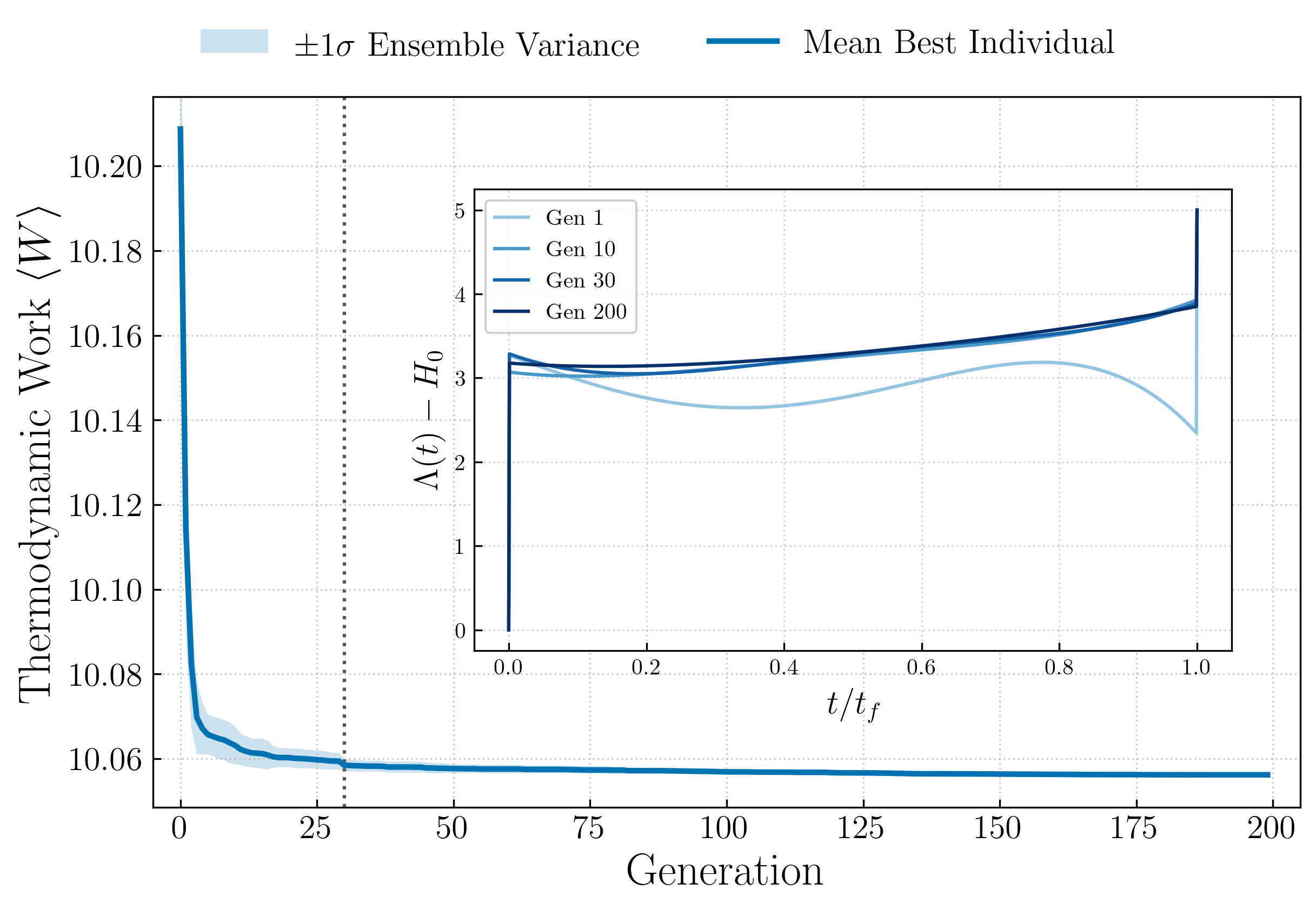
Fig. 8 shows the convergence history for the representative grid point $H_{0}=2$, $\alpha=25$. The best protocol from each trial is retrospectively evaluated at $100{,}000$ trajectories per generation using a shared fixed noise seed, a technique known as Common Random Numbers (CRN), which ensures that work values across trials and generations are directly comparable. The algorithm reaches a stable minimum by approximately generation 40, with negligible improvement thereafter.

Figure 9: Streamlines of fluid flow around a puller active particle near a no-slip wall. Panel (a) shows flow due to the source alone (flow in an unbounded domain). Panel (b) shows the flow due to image. Panel (c) is the net flow in the physical region ($z>0$). The image induces a drift of the puller active particle towards the wall. The corresponding plot for a pusher can be obtained by reversing the arrows.

Appendix C Fluid flow around an active particle near a wall

To enforce the no-slip boundary condition, we use the Method of images [20]. The solution is obtained in terms of a Green’s function - using method of images - that satisfies the no-slip boundary condition. A Green’s function of Stokes equation, which satisfies these properties, for a source at a height $h$ from the wall, can be written as [20, 36]: $G_{\alpha\beta}(\boldsymbol{R},\,\boldsymbol{R}^{\prime})=G_{\alpha\beta}^{0}(\boldsymbol{r})+G_{\alpha\beta}^{*}(\boldsymbol{R},\,\boldsymbol{R}^{*})$. Here $\boldsymbol{r}^{*}=\boldsymbol{R}-\boldsymbol{R}^{*}$ , $\boldsymbol{R}^{*}=\boldsymbol{\mathcal{M}}\cdot\boldsymbol{R^{\prime}}$ is the image at a distance $h$ from the wall at $z=0$. Note, $\boldsymbol{\mathcal{M}}=\boldsymbol{I}-2\boldsymbol{\hat{z}}\boldsymbol{\hat{z}}$. and ${G}^{0}_{\alpha\beta}(\boldsymbol{r})=\frac{1}{8\pi\eta}\left(\frac{\delta_{\alpha\beta}}{r}+\frac{r_{\alpha}r_{\beta}}{r^{3}}\right)$ is the Oseen tensor [36] with $r=|\boldsymbol{r}|=|\boldsymbol{R}-\boldsymbol{R}^{\prime}|$ and $\boldsymbol{G}^{*}$ is the correction necessary to satisfy the boundary condition [20]. The explicit form is: $G_{\alpha\beta}^{*}(\boldsymbol{R},\,\boldsymbol{R}^{*})=-G_{\alpha\beta}^{0}(\boldsymbol{r}^{*})-2h\nabla_{{\scriptscriptstyle\boldsymbol{r}_{\gamma}^{*}}}G_{\alpha 3}^{0}(\boldsymbol{r}^{*})\mathcal{M}_{\beta\gamma}+h^{2}\nabla_{{\scriptscriptstyle\boldsymbol{r}^{*}}}^{2}G_{\alpha\gamma}^{0}(\boldsymbol{r}^{*})\mathcal{M}_{\beta\gamma}.$ The expression of the flow created by a stresslet is given as a sum of contributions from the source and image $v^{\mathrm{net}}_{i}=v^{\mathrm{source}}_{i}+v^{\mathrm{image}}_{i}$, such that: $v^{\mathrm{source}}_{i}=-c_{2s}\bm{\nabla}_{\bm{R}^{\prime}}\bm{G}^{0}(\bm{R},\bm{R}^{\prime})\cdot\bm{S}$ and $v^{\mathrm{image}}_{i}=-c_{2s}\bm{\nabla}_{\bm{R}^{\prime}}\bm{G}^{*}(\bm{R},\bm{R}^{\prime})\cdot\bm{S}$. Here $S_{ij}=s_{0}(\hat{x}_{i}\hat{x}_{j}-\delta_{ij}/3)$, while $s_{0}$ and $c_{2s}$ are constants. The streamlines of the flow due to source, image, and net contributions is given in Fig.9.

References

- Peliti and Pigolotti [2021] L. Peliti and S. Pigolotti, Stochastic thermodynamics: an introduction (Princeton University Press, 2021).
- Shiraishi [2023] N. Shiraishi, An Introduction to Stochastic Thermodynamics (Springer, 2023).
- Seifert [2025] U. Seifert, Stochastic Thermodynamics (Cambridge University Press, 2025).
- Ashkin [2018] A. Ashkin, Nobel lecture: Optical tweezers and their application to biological systems (2018).
- Schmiedl and Seifert [2007] T. Schmiedl and U. Seifert, Optimal finite-time processes in stochastic thermodynamics, Phys. Rev. Lett. 98, 108301 (2007).
- Ramaswamy [2010] S. Ramaswamy, The Mechanics and Statistics of Active Matter, Annu. Rev. Condens. Mat. Phys. 1, 323 (2010).
- Marchetti et al. [2013] M. C. Marchetti, J. F. Joanny, S. Ramaswamy, T. B. Liverpool, J. Prost, M. Rao, and R. A. Simha, Hydrodynamics of soft active matter, Rev. Mod. Phys. 85, 1143 (2013).
- Vrugt et al. [2025] M. t. Vrugt, B. Liebchen, and M. E. Cates, What exactly is’ active matter’?, arXiv preprint arXiv:2507.21621 (2025).
- Garcia-Millan et al. [2025] R. Garcia-Millan, J. Schüttler, M. E. Cates, and S. A. Loos, Optimal closed-loop control of active particles and a minimal information engine, Phys. Rev. Lett. 135, 088301 (2025).
- Loos et al. [2024] S. A. Loos, S. Monter, F. Ginot, and C. Bechinger, Universal symmetry of optimal control at the microscale, Phys. Rev. X 14, 021032 (2024).
- Monter et al. [2025] S. Monter, S. A. Loos, and C. Bechinger, Optimal transitions between nonequilibrium steady states, PProc. Natl. Acad. Sci. 122, e2510654122 (2025).
- Zhong and DeWeese [2024] A. Zhong and M. R. DeWeese, Beyond linear response: Equivalence between thermodynamic geometry and optimal transport, Phys. Rev. Lett. 133, 057102 (2024).
- Davis et al. [2024] L. K. Davis, K. Proesmans, and É. Fodor, Active matter under control: Insights from response theory, Phys. Rev. X 14, 011012 (2024).
- Cocconi et al. [2023] L. Cocconi, J. Knight, and C. Roberts, Optimal power extraction from active particles with hidden states, Phys. Rev. Lett. 131, 188301 (2023).
- Casert and Whitelam [2024] C. Casert and S. Whitelam, Learning protocols for the fast and efficient control of active matter, Nature Communications 15, 9128 (2024).
- Gupta et al. [2023] D. Gupta, S. H. L. Klapp, and D. A. Sivak, Efficient control protocols for an active ornstein-uhlenbeck particle, Phys. Rev. E 108, 024117 (2023).
- Shankar et al. [2022] S. Shankar, V. Raju, and L. Mahadevan, Optimal transport and control of active drops, PProc. Natl. Acad. Sci. 119, e2121985119 (2022).
- Batchelor [1970] G. K. Batchelor, The stress system in a suspension of force-free particles, J. Fluid Mech. 41, 545 (1970).
- Lauga [2020] E. Lauga, The fluid dynamics of cell motility, Vol. 62 (Cambridge University Press, 2020).
- Blake [1971] J. R. Blake, A note on the image system for a Stokeslet in a no-slip boundary, Proc. Camb. Phil. Soc. 70, 303 (1971).
- Engel et al. [2023] M. C. Engel, J. A. Smith, and M. P. Brenner, Optimal control of nonequilibrium systems through automatic differentiation, Phys. Rev. X 13, 041032 (2023).
- Whitelam [2023] S. Whitelam, Demon in the machine: learning to extract work and absorb entropy from fluctuating nanosystems, Phys. Rev. X 13, 021005 (2023).
- Whitelam et al. [2025] S. Whitelam, C. Casert, M. Engel, and I. Tamblyn, Benchmark control problems in nonequilibrium statistical mechanics, arXiv preprint arXiv:2506.15122 (2025).
- Gardiner [1985] C. W. Gardiner, Handbook of stochastic methods (Springer Berlin, 1985).
- Kubo [1966] R. Kubo, The fluctuation-dissipation theorem, Rep. Prog. Phys. 29, 255 (1966).
- Brenner [1961] H. Brenner, The slow motion of a sphere through a viscous fluid towards a plane surface, Chem. Eng. Sci. 16, 242 (1961).
- Turk et al. [2024] G. Turk, R. Adhikari, and R. Singh, Fluctuating hydrodynamics of an autophoretic particle near a permeable interface, J. Fluid Mech. 998, A34 (2024).
- Sekimoto [1998] K. Sekimoto, Langevin equation and thermodynamics, Prog. Theor. Phys. Suppl. 130, 17 (1998).
- Gelfand and SV [2000] I. M. Gelfand and F. SV, Calculus of variations (Courier Corporation, 2000).
- Kikuchi et al. [2020] L. Kikuchi, R. Singh, M. E. Cates, and R. Adhikari, Ritz method for transition paths and quasipotentials of rare diffusive events, Phys. Rev. Res. 2, 033208 (2020).
- Boyd [2000] J. P. Boyd, Chebyshev and Fourier spectral methods (Dover, 2000).
- Kloeden and Platen [1992] P. E. Kloeden and E. Platen, Numerical solution of stochastic differential equations (Springer, 1992).
- Paszke et al. [2019] A. Paszke et al., Pytorch: An imperative style, high-performance deep learning library, in Advances in Neural Information Processing Systems 32 (2019) pp. 8024–8035.
- Alvarado et al. [2026] J. Alvarado, E. G. Teich, D. A. Sivak, and J. Bechhoefer, Optimal control in soft and active matter, Annu. Rev. Condens. Mat. Phys. 17 (2026).
- Goldstein [2015] R. E. Goldstein, Green algae as model organisms for biological fluid dynamics, Ann. Rev. Fluid Mech. 47, 343 (2015).
- Pozrikidis [1992] C. Pozrikidis, Boundary Integral and Singularity Methods for Linearized Viscous Flow (Cambridge University Press, 1992).