rSDNet: Unified Robust Neural Learning against Label Noise and Adversarial Attacks

Abstract

Neural networks are central to modern artificial intelligence, yet their training remains highly sensitive to data contamination. Standard neural classifiers are trained by minimizing the categorical cross-entropy loss, corresponding to maximum likelihood estimation under a multinomial model. While statistically efficient under ideal conditions, this approach is highly vulnerable to contaminated observations including label noises corrupting supervision in the output space, and adversarial perturbations inducing worst-case deviations in the input space. In this paper, we propose a unified and statistically grounded framework for robust neural classification that addresses both forms of contamination within a single learning objective. We formulate neural network training as a minimum-divergence estimation problem and introduce rSDNet, a robust learning algorithm based on the general class of $S$-divergences. The resulting training objective inherits robustness properties from classical statistical estimation, automatically down-weighting aberrant observations through model probabilities. We establish essential population-level properties of rSDNet, including Fisher consistency, classification calibration implying Bayes optimality, and robustness guarantees under uniform label noise and infinitesimal feature contamination. Experiments on three benchmark image classification datasets show that rSDNet improves robustness to label corruption and adversarial attacks while maintaining competitive accuracy on clean data, Our results highlight minimum-divergence learning as a principled and effective framework for robust neural classification under heterogeneous data contamination.

Keywords: Neural network classifier; robust learning; $S$-divergences; density power divergence; adversarial attacks; MLP; CNN.

1 Introduction

Deep neural networks form the backbone of modern machine learning and artificial intelligence (AI) systems, driving advances in vision, language, speech, healthcare, and autonomous decision-making. Their success is mainly due to the expressive power and universality of neural network (NN) architectures (Hornik et al.,, 1989), which facilitate flexible modeling of complex data structures. Training is commonly performed via empirical risk minimization on large-scale datasets, implicitly assuming that sample observations faithfully represent the underlying distribution and are free from contamination. As neural training is increasingly influencing high-stakes AI applications across industry and society, ensuring its robustness has become a foundational requirement for the stability, safety, and trustworthiness of modern AI systems.

In practice, however, training data are often contaminated, resulting in significantly poorer performance of neural learning systems. Two most prevalent sources of such corruption in neural classification are label noise and adversarial perturbations, affecting output and input spaces, respectively. Both distort empirical risk compromising the reliability and generalization. Although traditionally studied separately, they both may be viewed as structured forms of distributional contamination. This unified perspective motivates the central question of this work: can robustness to heterogeneous data deviations be achieved directly through a suitably defined training objective? Addressing this question, we develop a unified, statistically grounded minimum-divergence learning framework for neural classification, termed rSDNet, which provides inherent stability against both types of contamination within a single objective.

Learning with noisy labels has received substantial attention, motivated by annotation errors, weak supervision, crowd-sourced labeling, and large-scale web-based data collection. Neural classifiers are commonly trained using the categorical cross-entropy (CCE) loss, which corresponds to the maximum likelihood (ML) estimation under a multinomial model (Goodfellow et al.,, 2016). Due to inherent non-robustness of ML estimation, NNs trained with CCE loss tend to memorize mislabeled samples yielding poor generalization (Natarajan et al.,, 2013; Zhang et al.,, 2017). Existing solutions include loss correction methods that explicitly model or estimate noise transition mechanisms (Patrini et al.,, 2017), sample selection and reweighting strategies (Han et al.,, 2018; Ren et al.,, 2018), and alternative noise-robust loss functions, such as mean absolute error (MAE) and related losses (Ghosh et al., 2017b, ), generalized cross-entropy (GCE) of Zhang and Sabuncu, (2018), symmetric cross-entropy (SCE) based on the symmetric Kullback–Leibler divergence (Wang et al.,, 2019), trimmed CCE (TCCE) of Rusiecki, (2019), and fractional classification loss (FCL) of Kurucu et al., (2025). A comprehensive survey is available in Song et al., (2022). However, these approaches are primarily tailored to output-space label corruption and generally do not address adversarial perturbations in the input space.

Adversarial robustness addresses a structurally related vulnerability, namely small, carefully crafted input perturbations that induce high-confidence misclassification while remaining nearly imperceptible (Szegedy et al.,, 2013; Goodfellow et al.,, 2014). From a learning-theoretic perspective, such perturbations represent worst-case local deviations from the nominal data distribution, thereby constituting contamination in feature space. Adversarial training remains the dominant defense strategy, explicitly optimizing model parameters against worst-case perturbations within a prescribed norm ball (Madry et al.,, 2017). However, this approach typically incurs substantial computational overhead and may often reduce clean-data accuracy (Zhang et al.,, 2019; Rice et al.,, 2020). Related line of works includes certified robustness guarantees and distributionally robust optimization under bounded perturbations (Sinha et al.,, 2018; Cohen et al.,, 2019; Zhang et al.,, 2019). In this work, instead of attack-specific defenses, we develop a single principled robust loss that provides resilience across diverse adversarial perturbation strategies.

More broadly, robust NN learning has evolved along two primary methodological directions. The first modifies network architectures or training procedures to reduce sensitivity to corrupted observations. For example, regularization mechanisms such as dropout (Srivastava et al.,, 2014) have been shown to improve robustness against label noises in certain settings (Rusiecki,, 2020). The second adopts a more fundamental statistical viewpoint, constructing loss functions that down-weight aberrant observations, and is closely related to distributionally robust optimization against adversarial attacks. While these developments highlight the potential of statistically grounded objectives for mitigating contamination effects, most of the formal robust loss theory has been developed in regression contexts (Rusiecki,, 2007, 2013; Ghosh and Jana,, 2026), while those for classification are often tailored to specific corruption models (Qian et al.,, 2022). Consequently, a common training objective that simultaneously addresses both output- and input-space contamination within neural classification remains unexplored.

In this work, we formulate neural classification as a minimum-divergence estimation problem and propose a unified robust learning framework, termed rSDNet, based on the general class of $S$-divergences (Ghosh et al., 2017a, ). The $S$-divergence family provides a two-parameter formulation containing both the $\beta$-divergence (Basu et al.,, 1998) and the Cressie–Read power divergence (Cressie and Read,, 1984). It has been formally shown to yield highly efficient and robust statistical inference under potential data contamination (Ghosh,, 2015; Ghosh and Basu,, 2017). By translating these robustness properties to NN classification, rSDNet establishes a principled risk minimization strategy in which stability arises intrinsically from the curvature and influence down-weighting characteristics of the loss (divergence). Through theoretical analysis and controlled empirical experiments under both label corruption and adversarial perturbations, we demonstrate that robustness can emerge as an inherent property of the learning objective itself, rather than as an auxiliary defense mechanism.

The rest of the paper is organized as follows. The proposed rSDNet framework is developed in Section 2 along with necessary notations and assumptions. In Section 3, we establish key theoretical properties of rSDNet, including Fisher consistency and the classification calibration property justifying its Bayes optimality. Here we also investigate the theoretical robustness guarantees of rSDNet under both uniform label noises and infinitesimal contamination. Empirical studies on image classification tasks using three widely used benchmark datasets are presented in Section 4, which further support our theoretical findings. Finally, some concluding remarks are given in Section 5. All technical proofs, a discussion on the convergence rate of the proposed rSDNet algorithm, and detailed results from our numerical experiments are deferred to Appendices A–C.

2 The proposed robust learning framework

2.1 Model setup and notations

Consider a $J$-class classification problem with a set of $n$ independent training observations $\mathcal{S}_{n}=\{(\bm{y}_{i},\bm{x}_{i}):i=1,2,\ldots,n\}$, where $\bm{x}_{i}\in\mathcal{X}\subseteq\mathbb{R}^{p}$ denotes the $i$-th input feature vector and $\bm{y}_{i}=(y_{i1},\ldots,y_{iJ})^{\top}$ is the one-hot encoded categorical response vector indicating the class label of $\bm{x}_{i}$, for $i=1,\ldots,n$. Thus, $\bm{y}_{i}\in\mathcal{Y}=\{\bm{e}_{1},\bm{e}_{2},\ldots,\bm{e}_{J}\}$, where $\bm{e}_{j}$ denotes the $j$-th canonical basis vector in $\mathbb{R}^{J}$, and $\bm{y}_{i}=\bm{e}_{j}$ if and only if $\bm{x}_{i}$ belongs to class $j$, for each $i,j$. If we denote the random class label corresponding to $\bm{x}_{i}$ by $Y_{i}\in\{1,2,\ldots,J\}$, then we can also write $\bm{y}_{i}=\bm{e}_{Y_{i}}$ for each $i\geq 1$. Let us assume that the sampled observations $(\bm{y}_{i},\bm{x}_{i})$ are independent and identically distributed (IID) realizations of the underlying random vectors $(\bm{Y},\bm{X})$, and the conditional distribution of the one-hot encoded response $\bm{Y}$, given $\bm{X}=\bm{x}$, is Multinomial$(1;p_{1}^{\ast},\ldots,p_{J}^{\ast})$, where $p_{j}^{*}(\bm{x})=P(\bm{Y}=\bm{e}_{j}|\bm{X}=\bm{x})$ denotes the posterior probability of class $j=1,\ldots,J$. Throughout we assume that, given any $\bm{x}\in\mathcal{X}$, $\bm{p}^{*}(\bm{x})=(p_{1}^{\ast}(\bm{x}),\ldots,p_{J}^{*}(\bm{x}))^{\top}\in\Delta_{J}^{\circ}$, the interior of the probability simplex

$$\Delta_{J}=\left\{\bm{p}=(p_{1},\ldots,p_{J})^{\top}\in[0,1]^{J}:\sum_{j=1}^{J}p_{j}=1\right\}.$$

Our objective is to model the relationship between class probabilities and input features to facilitate classification of new observations. In neural classification, we employ an NN model with $J$ output nodes and a softmax activation to model the posterior class probabilities $p_{j}^{*}(\bm{x})$ by

$$p_{j}(\bm{x};\bm{\theta})=\frac{e^{z_{j}(\bm{x};\bm{\theta})}}{\sum_{k=1}^{J}e^{z_{k}(\bm{x};\bm{\theta})}},~~~~~j=1,\ldots,J,$$ (1)

where $z_{j}(\bm{x};\bm{\theta})$ denotes the pre-activation (net input) at the $j$-th output node, and $\boldsymbol{\theta}\in\Theta$ is the unknown model parameter consisting of all network weights and biases. The parameter space $\Theta$ depends on the assumed NN architecture. This model conditional distribution of $\bm{Y}$ given $\bm{X}$ is also Multinomial with class probabilities $\bm{p}(\bm{x};\bm{\theta})=(p_{1}(\bm{x};\bm{\theta}),\ldots,p_{J}(\bm{x};\bm{\theta}))^{\top}$, so that the model probability mass function (PMF) is given by

$$f_{\bm{\theta}}(\bm{u}|\bm{x})=\prod_{j=1}^{J}p_{j}^{u_{j}}(\bm{x};\bm{\theta}),~~~~~\bm{u}=(u_{1},\ldots,u_{J})^{\top}\in\mathcal{Y}.$$ (2)

If we denote an estimator of $\bm{\theta}$ obtained from the training sample $\mathcal{S}_{n}$ by $\widehat{\bm{\theta}}_{n}$, the resulting plug-in classification rule (NN classifier) is given by $\delta_{n}(\bm{x})=\arg\max\limits_{1\leq j\leq J}p_{j}(\bm{x};\widehat{\bm{\theta}}_{n})$.

In practice, the parameter vector $\bm{\theta}$ for an NN classifier is commonly estimated by minimizing the CCE loss function given by

$$\mathcal{L}_{0}(\bm{\theta})=-\frac{1}{n}\sum_{i=1}^{n}\sum_{j=1}^{J}y_{ij}\ln{p_{j}(\bm{x}_{i};\bm{\theta})},$$ (3)

which coincides with the ML estimation of the model parameters under the multinomial PMF in (2). Consequently, the resulting classifier inherits the well-known sensitivity of ML methods to any form of data contamination and model misspecification.

2.2 Minimum divergence learning framework

The equivalence between CCE-based training and ML estimation naturally places neural classification within the broader framework of minimum divergence estimation (MDE). Statistical MDE provides a principled approach to parameter estimation, where estimators are obtained by minimizing a divergence between the empirical distribution and a parametric model, with the choice of divergence determining their properties. Historically, divergence-based estimation can be traced back to Pearson’s chi-squared divergence, one of the earliest theoretically grounded approaches to statistical inference. In recent decades, divergence-based methods have received renewed attention due to their ability to produce robust estimators with little or no loss in pure data efficiency when an appropriate divergence is selected; see, e.g, Basu et al., (2011).

To formalize this framework in the present setting of NN classification (Section 2.1), let $g(\bm{u}|\bm{x})$, $\bm{u}\in\mathcal{Y}$, denotes the true conditional PMF of $\bm{Y}$ given $\bm{X}=\bm{x}\in\mathcal{X}$, corresponding to the Multinomial distribution with true class probabilities $\bm{p}^{\ast}(\bm{x})$, for each $i=1,\ldots,n$. Its empirical counterpart at the observed feature values is directly obtained as $\widehat{g}_{i}(\bm{u}):=\widehat{g}(\bm{u}|\bm{x}_{i})=\mathbb{I}(\bm{u}=\bm{y}_{i})$ for $\bm{u}\in\mathcal{Y}$ and $i=1,\ldots,n$, where $\mathbb{I}(\cdot)$ denotes the indicator function. Without assuming any model distribution for $\bm{X}$, here we are basically modelling each conditional PMF $g_{i}=g(\cdot|\bm{x}_{i})$ by the parametric PMF $f_{i,\bm{\theta}}=f_{\bm{\theta}}(\cdot|\bm{x}_{i})$, as given in (2), over observed feature values $\bm{x}_{i}$, $i=1,\ldots,n$. Thus, a general minimum divergence estimator $\widehat{\bm{\theta}}_{n}$ of $\bm{\theta}$, with respect to a statistical divergence measure $d(\cdot,\cdot)$, is defined as $\widehat{\bm{\theta}}_{n}=\operatorname*{arg\,min}_{\bm{\theta}}\frac{1}{n}\sum_{i=1}^{n}d\bigl(\widehat{g}_{i},f_{i,\bm{\theta}}\bigr).$

In particular, the ML estimation corresponds to the MDE based on the Kullback–Leibler divergence (KLD) $d_{\mathrm{KL}}(\cdot,\cdot)$. A straightforward calculation yields

$$d_{\mathrm{KL}}(\widehat{g}_{i},f_{i,\bm{\theta}})=\sum\limits_{\bm{u}\in\mathcal{Y}}\widehat{g}_{i}(\bm{u})\log\frac{\widehat{g}_{i}(\bm{u})}{f_{i,\bm{\theta}}(\bm{u})}=-\sum_{j=1}^{J}y_{ij}\log p_{j}(\bm{x}_{i};\bm{\theta}),$$

since $\widehat{g}_{i}(\bm{e}_{j})=y_{ij}$ for all $i,j\geq 1$, and hence $\sum_{\bm{u}}\widehat{g}_{i}(\bm{u})\log\widehat{g}_{i}(\bm{u})=\sum_{j}y_{ij}\log y_{ij}=0$ under one-hot encoding (with the convention $0\cdot\log 0=0$). Consequently, the CCE loss in (3) can be expressed as the average KLD measure $\frac{1}{n}\sum_{i=1}^{n}d_{\mathrm{KL}}(\widehat{g}_{i},f_{i,\bm{\theta}})$, Hence, minimizing the CCE loss is exactly equivalent to minimizing the average KLD between the empirical and model conditional PMFs.

This characterization motivates a general minimum divergence learning framework for neural classifiers, where the KLD may be replaced by a suitably chosen alternative divergence to achieve desirable statistical properties. In particular, divergences possessing suitable robustness properties can substantially mitigate the sensitivity of ML-based training to contamination and model misspecification. Here we adopt the particular class of $S$-divergences (Ghosh et al., 2017a, ) to construct our proposed rSDNet, yielding enhanced robustness under both input- and output-space contamination while retaining high statistical efficiency under clean data.

2.3 $S$-Divergence family and the rSDNet objective

As introduced by Ghosh et al., 2017a , the $S$-divergence (SD) between two PMFs, $g$ and $f$ having common support $\mathcal{Y}$ is defined, depending on two tuning parameters $\beta\geq 0$ and $\lambda\in\mathbb{R}$, as

$$S_{\beta,\lambda}(g,f)=\frac{1}{A}\sum_{\bm{u}\in\mathcal{Y}}f^{1+\beta}(\bm{u})-\frac{1+\beta}{AB}\sum_{\bm{u}\in\mathcal{Y}}f^{B}(\bm{u})g^{A}(\bm{u})+\frac{1}{B}\sum_{\bm{u}\in\mathcal{Y}}g^{1+\beta}(\bm{u}),$$

where $A=1+\lambda(1-\beta)\neq 0$, and $B=\beta-\lambda(1-\beta)\neq 0$. When either $A=0$ or $B=0$, the corresponding SD measures are defined through respective continuous limits. The tuning parameters $(\beta,\lambda)$ control the robustness–efficiency trade-off of the resulting MDE and associated inference. Particularly, $\beta$ adjusts the influence of outlying observations, so that larger $\beta$ increases robustness but reduces efficiency; values of $\beta>1$ are typically avoided due to severe efficiency loss. On the other hand, $\lambda$ interpolates between divergence families allowing further (higher-order) control over robustness while preserving the same first-order asymptotic efficiency at a fixed $\beta$. However, Ghosh et al., 2017a demonstrated that the minimum SD estimators (MSDEs) exhibit good robustness only when $A\geq 0$. Recently, Roy et al., (2026) established the asymptotic breakdown point of the MSDEs and associated functionals, confirming high-robustness when $A\geq 0$ and $B\geq 0$. Both studies further suggest that the best robustness–efficiency trade-offs are obtained for appropriate SD measures with $A>0$ and $B>0$. Thus, excluding the boundary cases $A=0$ or $B=0$, here we restrict ourselves to the SDs with admissible tuning parameters satisfying $A>0$ and $B>0$, namely

$$\mathcal{T}=\left\{(\beta,\lambda):-\frac{1}{1-\beta}<\lambda<\frac{\beta}{1-\beta},0\leq\beta<1\right\}\cup\bigg\{(1,\lambda):\lambda\in\mathbb{R}\bigg\}.$$

Note that the second part of $\mathcal{T}$ corresponds to a single divergence, since the SD reduces to the squared $L_{2}$ distance at $\beta=1$, irrespective of $\lambda$. Despite this restriction, $\mathcal{T}$ retains most important subclasses of the SD family. The choice $\lambda=0$ produces $\beta$-divergences or density power divergences (DPDs) of Basu et al., (1998), while $\beta=0$ gives the power divergence (PD) family (Cressie and Read,, 1984) with $-1<\lambda<0$, including the Hellinger disparity at $\lambda=-0.5$. However, the set $\mathcal{T}$ exclude the non-robust KLD at $(\beta,\lambda)=(0,0)$ and the reverse KLD (rKLD) at $(\beta,\lambda)=(0,-1)$, the latter known to cause computational difficulties in discrete models with inliers (Basu et al.,, 2011). More broadly, the SD family can be viewed as a reparameterization of $(\alpha,\beta)$-divergences (Cichocki et al.,, 2011) and also as a special case of extended Bregman divergences of Basak and Basu, (2022).

Under our setup of neural classification given in Section 2.1, and following the general discussions in Section 2.2, we define the MSDE of the NN model parameter $\boldsymbol{\theta}$ as

$$\widehat{\bm{\theta}}_{n}^{(\beta,\lambda)}=\arg\min_{\bm{\theta}\in\Theta}\mathcal{L}_{\beta,\lambda}^{(n)}(\bm{\theta}),~~~~\mbox{ with }~~\mathcal{L}_{\beta,\lambda}^{(n)}(\bm{\theta})=\frac{1}{n}\sum_{i=1}^{n}S_{\beta,\lambda}(\widehat{g}_{i},f_{i,\bm{\theta}}).$$ (4)

We refer to the resulting neural classifier trained via an MSDE $\widehat{\bm{\theta}}_{n}^{(\beta,\lambda)}$ as rSDNet$(\beta,\lambda)$ for any given choice of $(\beta,\lambda)\in\mathcal{T}$, and the associated objective function $\mathcal{L}_{\beta,\lambda}^{(n)}(\bm{\theta})$ as rSDNet loss (empirical SD-risk) or rSDNet training objective. We next study this loss function further to develop a scalable practical implementation of rSDNet.

2.4 The final rSDNet learning algorithm

For practical implementation of rSDNet, the associated NN training objective $\mathcal{L}_{\beta,\lambda}^{(n)}(\bm{\theta})$ can be expressed in a much simplified form. Substituting the explicit forms of $\widehat{g}_{i}$ and $f_{i,\bm{\theta}}$ into the SD expression (2.3), we obtain the final rSDNet training objective (loss) as given by

$$\mathcal{L}_{\beta,\lambda}^{(n)}(\bm{\theta})=\frac{1}{n}\sum_{i=1}^{n}\ell_{\beta,\lambda}(\bm{y}_{i},\bm{p}(\bm{x}_{i};\bm{\theta})),~~~~~(\beta,\lambda)\in\mathcal{T},$$ (5)

$$\mbox{where }~~~\ell_{\beta,\lambda}(\bm{u},\bm{p})=\displaystyle\frac{1}{A}\sum_{j=1}^{J}\left[p_{j}^{1+\beta}-\frac{1+\beta}{B}u_{j}p_{j}^{B}+\frac{A}{B}\right],~~~\mbox{ for }~(\beta,\lambda)\in\mathcal{T},~\bm{u}\in\mathcal{Y},~\bm{p}\in\Delta_{J}.~~~$$ (6)

Although we restrict ourselves to tuning parameter values in $\mathcal{T}$, the rSDNet loss $\mathcal{L}_{\beta,\lambda}(\bm{\theta})$ can also be extended to the boundary cases of $A=0$ or $B=0$ by the respective continuous limits of the form given in (5)–(6). We avoided these boundary cases as they are expected to have practical issues with either outliers or inliers (Ghosh et al., 2017a, ).

Since the rSDNet objective $\mathcal{L}_{\beta,\lambda}(\bm{\theta})$ in (5) can be non-convex in $\bm{\theta}$ by the choice of the network architecture in $\bm{p}(\bm{x};\bm{\theta})$, following standard NN learning procedures, we propose to solve this optimization problem efficiently using the Adam algorithm (Kingma and Ba,, 2014). It is a first-order stochastic gradient method, which starts with initializing two moment vectors $\bm{m}_{0}$ and $\bm{v}_{0}$ to the null vector, and update the minimizer of $\mathcal{L}_{\beta,\lambda}(\bm{\theta})$ at the $t$-th step of iteration by

$$\bm{\theta}_{t}\leftarrow\bm{\theta}_{t-1}-\alpha\ \bm{\widehat{m}}_{t}/\left(\sqrt{\bm{\widehat{v}}_{t}}+\epsilon\right),~~~~t=1,2,\ldots,$$ (7)

where $\bm{\widehat{m}}_{t}$ and $\bm{\widehat{v}}_{t}$ are, respectively, the updated bias-corrected estimates of first and second raw moments, given by

$$\bm{\widehat{m}}_{t}\leftarrow\frac{\beta_{1}\bm{m}_{t-1}+(1-\beta_{1})\bm{g}_{t}}{1-\beta_{1}^{t}},~~\bm{\widehat{v}}_{t}\leftarrow\frac{\beta_{2}\bm{v}_{t-1}+(1-\beta_{2})\bm{g}_{t}^{2}}{1-\beta_{2}^{t}},$$

with $\bm{g}_{t}=\nabla_{\bm{\theta}}\mathcal{L}_{\beta,\lambda}(\bm{\theta}_{t-1})$ denoting the gradient of the loss function with respect to $\bm{\theta}$, and $\bm{g}_{t}^{2}$ being the vector of squared elements of $\bm{g}_{t}$ for each $t\in\mathbb{N}$. Given the form of the rSDNet loss function in (5)–(6), we can compute its gradient as given by

$$\nabla_{\bm{\theta}}\mathcal{L}_{\beta,\lambda}(\bm{\theta})=\displaystyle\frac{1+\beta}{nA}\sum_{i=1}^{n}\sum_{j=1}^{J}\left[p_{j}^{\beta}(\bm{x}_{i};\bm{\theta})-y_{ij}p_{j}^{B-1}(\bm{x}_{i};\bm{\theta})\right]\nabla_{\bm{\theta}}p_{j}(\bm{x}_{i};\bm{\theta}),~~~~~(\beta,\lambda)\in\mathcal{T}.$$ (8)

For NN architectures involving non-smooth activation functions (e.g., ReLU), its output $p_{j}(\bm{x}_{i};\bm{\theta})$ might not be differentiable everywhere with respect to $\bm{\theta}$. In such cases, we need to replace $\nabla_{\bm{\theta}}p_{j}(\cdot;\bm{\theta})$ in gradient computation by a measurable selection from its subdifferential $\partial_{\bm{\theta}}p_{j}(\cdot,\bm{\theta})$, which is assumed to exist for most commonly used NN architectures.

For efficient implementation of the Adam algorithm, we have used the TensorFlow library (Abadi et al.,, 2016) of Python,; it computes the required gradient $\bm{g}_{t}$ via automatic differentiation (Bolte and Pauwels,, 2021), covering the cases of non-smooth activation as well. As initial weights $\bm{\theta}_{0}$ in the training process, we have used either of the standard built-in initializers ‘Glorot’ and ‘He’, which correspond to the normal and uniform base distributions, respectively. Throughout our empirical experimentation, we have used the default Adam hyperparameter values suggested by Kingma and Ba, (2014), which are $\alpha=10^{-3}$, $\beta_{1}=0.9$, $\beta_{2}=0.999$, and $\epsilon=10^{-8}$. Python codes for the complete rSDNet training are available through the GitHub repository Robust-NN-learning.

Following the theory of Adam (Kingma and Ba,, 2014), one should ideally continue the iterative updation step (7) until the sequence $\{\bm{\theta}_{t}\}$ converges. However, in most practical problems, achieving such full convergence is often computationally expensive. So, Adam updates are typically executed for a predefined number of epochs, which is generally chosen by monitoring the stability of the test accuracy for the trained classifier. In all illustration presented in this paper, we employed the Adam algorithm for 250 epochs, which was observed to be sufficient for stable training of rSDNet; see Appendix B for an empirical study justifying it for both pure and contaminated data.

3 Theoretical guarantees

3.1 Statistical consistency of rSDNet functionals

We start by establishing that the proposed rSDNet classifier indeed defines a valid statistical classification rule at the population level, which is essential for justifying its use in learning from random training samples under ideal conditions. In this respect, we need to define the population-level functionals associated with rSDNet, which characterizes the target parameters that empirical learning procedures aim to estimate.

We may note that the MSDE $\widehat{\bm{\theta}}_{n}^{(\beta,\lambda)}$ of the NN model parameter $\boldsymbol{\theta}$ under rSDNet$(\beta,\lambda)$ may be re-expressed from (4) as a minimizer of $E_{G_{\bm{X},n}}[S_{\beta,\lambda}(\widehat{g}(\cdot|\bm{X}),f_{\bm{\theta}}(\cdot|\bm{X}))]$ with respect to $\bm{\theta}\in\Theta$, where $G_{\bm{X},n}$ denotes the empirical distribution function of $\bm{X}$ placing mass $1/n$ at each observed $\bm{x}_{i}$, and $\widehat{g}$ is the empirical estimate of $g$ based on the training sample $\mathcal{S}_{n}$. Accordingly, we define the population-level minimum SD functional (MSDF) of $\bm{\theta}$ for tuning parameters $(\beta,\lambda)\in\mathcal{T}$ at the true distributions $(G_{\bm{X}},g)$ as

$$\bm{T}_{\beta,\lambda}(G_{\bm{X}},g)=\operatorname*{arg\,min}\limits_{\bm{\theta}\in\Theta}\mathcal{R}_{\beta,\lambda}(\bm{\theta}|G_{\bm{X}},g)~~~\mbox{ with }~~\mathcal{R}_{\beta,\lambda}(\bm{\theta}|G_{\bm{X}},g)=E_{G_{\bm{X}}}\left[S_{\beta,\lambda}(g(\cdot|\bm{X}),f_{\bm{\theta}}(\cdot|\bm{X}))\right],$$ (9)

where $G_{\bm{X}}$ denotes the true distribution function of $\bm{X}$ and $\mathcal{R}_{\beta,\lambda}(\bm{\theta})=\mathcal{R}_{\beta,\lambda}(\bm{\theta}|G_{\bm{X}},g)$ is the population SD-risk. At the empirical level, this corresponds to $\mathcal{R}_{\beta,\lambda}(\bm{\theta}|G_{\bm{X},n},\widehat{g})=\mathcal{L}_{\beta,\lambda}^{(n)}(\bm{\theta})$, so that $\bm{T}_{\beta,\lambda}(G_{\bm{X},n},\widehat{g})=\widehat{\bm{\theta}}_{n}^{(\beta,\lambda)}$. We refer to the resulting neural classifier obtained by setting $\bm{\theta}=\bm{T}_{\beta,\lambda}(G_{\bm{X}},g)$ as the rSDNet functional. The following theorem then presents its Fisher consistency; the proof is straightforward from the fact that SD is a genuine statistical divergence (Ghosh et al., 2017a, ).

Theorem 3.1 (Fisher Consistency of rSDNet).

For any $(\beta,\lambda)\in\mathcal{T}$, the posterior class probabilities of the rSDNet functional, obtained using the MSDF in (9), satisfy

$$\bm{p}(\bm{x};\bm{T}_{\beta,\lambda}(G_{\bm{X}},g))=\bm{p}(\bm{x};\bm{\theta}_{0})=\bm{p}^{*}(\bm{x})\quad\text{a.s.},$$

for any marginal distribution $G_{\bm{X}}$, provided that the conditional model is correctly specified with $g\equiv f_{\bm{\theta}_{0}}$ for some $\bm{\theta}_{0}\in\Theta$.

The above theorem shows Fisher consistency and uniqueness of the rSDNet functional at the level of class probabilities. A similar result for the MSDF $\bm{T}_{\beta,\lambda}(G_{\bm{X}},g)$ requires the following standard identifiability condition for the assumed NN architecture.

1. The NN classifier output function $\bm{x}\mapsto\bm{p}(\bm{x};\bm{\theta})$ is measurable for all $\bm{\theta}\in\Theta$, and the parameterization $\bm{\theta}\mapsto\bm{p}(\bm{x};\bm{\theta})$ is identifiable in $\bm{\theta}$ up to known network symmetries, i.e.,

   $$\bm{p}(\bm{x};\bm{\theta}_{1})=\bm{p}(\bm{x};\bm{\theta}_{2})~~a.s.~~~~~\Rightarrow~~~\bm{\theta}_{1}=\mathbb{g}\cdot\bm{\theta}_{2},$$

   for some $\mathbb{g}$ in a known symmetry group $\mathcal{G}$ acting on the (non-empty) parameter space $\Theta$.

Under Assumption (A0), the MSDF at any $(\beta,\lambda)\in\mathcal{T}$ satisfies $\bm{T}_{\beta,\lambda}(G_{\bm{X}},g)=\mathbb{g}\cdot\bm{\theta}_{0}$ for some $\mathbb{g}\in\mathcal{G}$ as in (A0). Thus, $\bm{T}_{\beta,\lambda}(G_{\bm{X}},g)$ is unique only up to known NN symmetries, which is consistent with standard NN learning theory (see, e.g., Goodfellow et al.,, 2016; Ghosh and Jana,, 2026).

Beyond Fisher consistency, the rSDNet functional is also classification-calibrated, meaning that minimization of the population SD-risk $\mathcal{R}_{\beta,\lambda}(\bm{\theta})$ yields Bayes-optimal classification decisions at the population level (Zhang,, 2004; Bartlett et al.,, 2006; Tewari and Bartlett,, 2007). To verify this, let us further simplify the population SD-risk, using the form of SD given in (2.3), as $\mathcal{R}_{\beta,\lambda}(\bm{\theta})=E_{G_{\bm{X}}}\left[r_{\beta,\lambda}(p^{*}(\bm{X}),p(\bm{X};\bm{\theta}))\right],$ where we define the conditional SD-risk

$$r_{\beta,\lambda}(\bm{p}^{*},\bm{p})=\frac{1}{A}\sum_{j=1}^{J}\left[p_{j}^{1+\beta}-\frac{1+\beta}{B}p_{j}^{B}{p_{j}^{*}}^{A}+\frac{A}{B}{p_{j}^{*}}^{1+\beta}\right],\qquad\mbox{for }~(\beta,\lambda)\in\mathcal{T},~\bm{p},\bm{p}^{*}\in\Delta_{J}.$$ (10)

Note that $r_{\beta,\lambda}(\bm{u},\bm{p})=\ell_{\beta,\lambda}(\bm{u},\bm{p})$ for any $\bm{u}\in\mathcal{Y}$ and $\bm{p}\in\Delta_{J}$, although they differ for any $\bm{p}^{*}\in\Delta_{J}^{\circ}$ unless $(\beta,\lambda)=(0,-1)$. Further, since (10) corresponds to the SD between $\bm{p}^{*}$ and $\bm{p}$, it is always non-negative and equals zero if and only if $\bm{p}=\bm{p}^{*}$. Consequently, the population SD-risk $\mathcal{R}_{\beta,\lambda}(\bm{\theta})$ has a unique minimizer at $\bm{p}=\bm{p}^{*}$ for any $(\beta,\lambda)\in\mathcal{T}$. In other words, the SD-loss underlying rSDNet is classification-calibrated in the sense of Bartlett et al., (2006). Hence, the class predicted by the rSDNet functional coincides with that of the asymptotically optimal Bayes classifier, $\delta_{B}(\bm{x})=\arg\max_{1\leq j\leq J}p_{j}^{*}(\bm{x})$, which minimizes the conditional misclassification risk. These properties of rSDNet are summarized in the following theorem.

Theorem 3.2 (Classification calibration of rSDNet).

The rSDNet functional at any $(\beta,\lambda)\in\mathcal{T}$ is classification-calibrated, and hence the induced classifier achieves the Bayes-optimal class prediction at the population level.

3.2 Tolerance against uniform label noise

We now establish the robustness of rSDNet against uniform label noise, a widely used output noise model in classification. Each training label is assumed to be independently corrupted with probability $\eta\in[0,1]$; when corruption occurs, the label is replaced uniformly at random by one of the remaining class labels. Formally, we represent contaminated training data as $\mathcal{S}_{\eta}=\{(\widetilde{\bm{y}}_{i},\bm{x}_{i}):i=1,2,\ldots,n\}$, where the observed label $\widetilde{\bm{y}}_{i}=\bm{y}_{i}$ with probability $1-\eta$ and equals any incorrect class label with probability $\eta/(J-1)$ when the input feature value is $\bm{x}_{i}$, $i\geq 1$. If we denote the random variable corresponding to $\widetilde{\bm{y}}_{i}$ by $\widetilde{\bm{Y}}$, then the true conditional distribution of $\widetilde{\bm{Y}}$, given $\bm{X}=\bm{x}$, is again Multinomial but with PMF $g_{\eta}(\cdot|\bm{x})$ involving class probabilities $\bm{p}_{\eta}^{*}(\bm{x})=(p_{\eta,1}^{*}(\bm{x}),\ldots,p_{\eta,J}^{*}(\bm{x}))$, where

$$p_{\eta,j}^{*}(\bm{x})=(1-\eta)p_{j}^{*}(\bm{x})+\frac{\eta}{J-1}(1-p_{j}^{*}(\bm{x})),~~~~~j=1,\ldots,J.$$

We study the effect of such noise on the expected SD-loss underlying our rSDNet, given by

$$R_{\beta,\lambda}(\bm{\theta})=E_{(\bm{Y},\bm{X})}\left[\mathcal{L}_{\beta,\lambda}^{(n)}(\bm{\theta})\right]=E_{(\bm{Y},\bm{X})}\left[\ell_{\beta,\lambda}(\bm{Y},\bm{p}(\bm{X};\bm{\theta}))\right]=E_{G_{\bm{X}}}\left[E_{g}\left[\ell_{\beta,\lambda}(\bm{Y},\bm{p}(\bm{X};\bm{\theta}))|\bm{X}\right]\right].$$

Let $\bm{\theta}_{\beta,\lambda}^{*}$ denotes its global minimizer at $(\beta,\lambda)\in\mathcal{T}$. We compare the minimum achievable expected SD-loss $R_{\beta,\lambda}(\bm{\theta}_{\beta,\lambda}^{*})$ under clean data with that obtained under uniform label noise. To this end, we define $\bm{\theta}_{\beta,\lambda}^{\eta}$ to be the global minimizer of the expected SD-risk under uniform label noise, given by

$$R_{\beta,\lambda}^{\eta}(\bm{\theta})=E_{(\widetilde{\bm{Y}},\bm{X})}\left[\mathcal{L}_{\beta,\lambda}^{(n)}(\bm{\theta})\right]=E_{G_{\bm{X}}}\left[E_{g_{\eta}}\left[\ell_{\beta,\lambda}(\bm{Y},\bm{p}(\bm{X};\bm{\theta}))|\bm{X}\right]\right].$$

Then we assess the robustness of rSDNet through the excess risk, $R_{\beta,\lambda}(\bm{\theta}_{\beta,\lambda}^{\eta})-R_{\beta,\lambda}(\bm{\theta}_{\beta,\lambda}^{*})$. Smaller this difference close to zero, greater the tolerance of rSDNet against uniform label noises. To derive a bound for it, we first show the uniform boundedness of the total SD-loss in the following lemma; its proof is given in Appendix A.1.

Lemma 3.3.

For any $\bm{x}\in\mathcal{X}$, $\bm{\theta}\in\Theta$, and $(\beta,\lambda)\in\mathcal{T}$, we have

$$\frac{J^{1-\beta}}{A}-\frac{1+\beta}{AB}\max(1,J^{1-B})+\frac{J^{2}}{B}\;\leq\;\sum_{j=1}^{J}\ell_{\beta,\lambda}(\bm{e}_{j},\bm{p}(\bm{x};\bm{\theta}))\;\leq\;\frac{J}{A}-\frac{1+\beta}{AB}\min(1,J^{1-B})+\frac{J^{2}}{B}.$$ (11)

Since the total SD-loss in Lemma 3.3 depends on $(\bm{x},\bm{\theta})$, it is not symmetric in the sense of Ghosh et al., 2017b . Symmetry arises only at $(\beta,\lambda)=(0,-1)$, corresponding to the rKLD having $A=0$, which lies outside our admissible parameter range $\mathcal{T}$; see Wang et al., (2019) for neural classifiers developed based on the rKLD and its practical limitations.

Although SD-loss is not symmetric and thus not exactly noise-tolerant, rSDNet still exhibits bounded excess risk under uniform label noise for all $(\beta,\lambda)\in\mathcal{T}$. The exact bound is provided in the following theorem; see Appendix A.2 for its proof.

Theorem 3.4.

Under uniform label noise with contamination proportion $0\leq\eta<1-1/J$, the excess risk of rSDNet satisfies

$$0\leq R_{\beta,\lambda}(\bm{\theta}_{\beta,\lambda}^{\eta})-R_{\beta,\lambda}(\bm{\theta}_{\beta,\lambda}^{*})\leq M_{\beta,\lambda}^{(\eta)},~~~~(\beta,\lambda)\in\mathcal{T},$$ (12)

where

$$M_{\beta,\lambda}^{(\eta)}=\frac{\eta}{(J-1-J\eta)}\frac{1}{A}\left(J-J^{1-\beta}+\frac{1+\beta}{B}|1-J^{1-B}|\right).$$

Note that the bound $M_{\beta,\lambda}^{(\eta)}$ in Theorem 3.4 decomposes into two components: one depending on the noise level $\eta$ and the other on the tuning parameters $(\beta,\lambda)$. The $\eta$-dependent factor coincides with that obtained in robust learning literature (e.g., Ghosh et al., 2017b, ), implying the same rate of degradation with increasing noise. In particular, the bound vanishes as $\eta\downarrow 0$ and diverges as $\eta\uparrow(J-1)/J$. The second component in $M_{\beta,\lambda}^{(\eta)}$ quantifies the effect of $(\beta,\lambda)$ and explains the improved robustness of certain rSDNet members. For fixed $(\eta,J)$, the bound decreases as $\beta$ increases, indicating greater tolerance to uniform label noise (see Figure 1). The role of $\lambda$ becomes more pronounced at higher contamination levels; for any fixed $\beta\in[0,1]$, the bound is minimized when $\lambda\in[-1,0]$ and increases rapidly as $\lambda$ moves outside this range.

(a) $\eta=0.2$

(b) $\eta=0.4$

(c) $\eta=0.6$

Figure 1: Plots of the bound $M_{\beta,\lambda}^{\eta}$ on the excess risk of rSDNet, as a function of tuning parameters $(\beta,\lambda)$, for different contamination proportion $\eta$ and $J=10$.

3.3 Local robustness against contaminated features

We next evaluate the local robustness of rSDNet to infinitesimal contamination in the feature space using influence function (IF) analysis. Since sample-based IFs are often difficult to interpret in deep learning settings (see, e.g., Basu et al.,, 2021; Bae et al.,, 2022), we adopt the population-level formulation of IF as originally introduced by Hampel et al., (1986). Specifically, we study the IF of the MSDF $\bm{T}_{\beta,\lambda}(G_{\bm{X}},g)$ underlying our rSDNet, under a gross-error contaminated feature distribution $G_{\bm{X},\epsilon}=(1-\epsilon)G_{\bm{X}}+\epsilon\wedge_{\bm{x}_{t}}$, where $\epsilon>0$ denotes the contamination proportion at an outlying point $\bm{x}_{t}\in\mathcal{X}$ and $\wedge_{\bm{x}}$ denotes the degenerate distribution at $\bm{x}\in\mathcal{X}$. The IF of $\bm{T}_{\beta,\lambda}$ at the contamination point $\bm{x}_{t}$ is formally defined as

$$\mathcal{IF}(\bm{x}_{t},\bm{T}_{\beta,\lambda},(G_{\bm{X}},g))=\lim\limits_{\epsilon\downarrow 0}\frac{\bm{T}_{\beta,\lambda}(G_{\bm{X}},g)-\bm{T}_{\beta,\lambda}(G_{\bm{X},\epsilon},g)}{\epsilon}=\frac{\partial}{\partial\epsilon}\bm{T}_{\beta,\lambda}(G_{\bm{X},\epsilon},g)\bigg|_{\epsilon=0},$$

which quantifies the effect of infinitesimal contamination at $\bm{x}_{t}$ on the resulting estimator and hence on the rSDNet framework.

In order to derive the expression of this IF at any $(\beta,\lambda)\in\mathcal{T}$, we define

$$\bm{\psi}_{\beta,\lambda}(\bm{x};\bm{\theta}) = \frac{A}{1+\beta}\nabla_{\bm{\theta}}\left[r_{\beta,\lambda}(\bm{p}^{*}(\bm{x}),\bm{p}(\bm{x};\bm{\theta}))\right]=\sum_{j=1}^{J}u_{j}(\bm{x};\bm{\theta})\nabla_{\bm{\theta}}p_{j}(\bm{x};\bm{\theta}),$$ (13)

with $$u_{j}(\bm{x};\bm{\theta})=p_{j}^{\beta}(\bm{x};\bm{\theta})-{p_{j}^{*}}^{A}(\bm{x})p_{j}^{B-1}(\bm{x};\bm{\theta}),$$

$$\mbox{and }~~~\bm{\Psi}_{\beta,\lambda}(\bm{\theta}) = \frac{A}{1+\beta}\nabla_{\bm{\theta}}^{2}\mathcal{R}_{\beta,\lambda}(\bm{\theta})=E_{G_{\bm{X}}}\left[\nabla_{\bm{\theta}}\bm{\psi}_{\beta,\lambda}(\bm{X};\bm{\theta})\right],$$ (14)

$$= E_{G_{\bm{X}}}\left[\sum_{j=1}^{J}u_{j}^{\prime}(\bm{X};\bm{\theta})\nabla_{\bm{\theta}}p_{j}(\bm{X};\bm{\theta})\nabla_{\bm{\theta}}^{\top}p_{j}(\bm{X};\bm{\theta})+\sum_{j=1}^{J}u_{j}(\bm{X};\bm{\theta})\nabla_{\bm{\theta}}^{2}p_{j}(\bm{X};\bm{\theta})\right],~~~~~~~~$$

with $$u_{j}^{\prime}(\bm{x};\bm{\theta})=\beta p_{j}^{\beta-1}(\bm{x};\bm{\theta})-{p_{j}^{*}}^{A}(\bm{x})(B-1)p_{j}^{B-2}(\bm{x};\bm{\theta}).$$

As noted earlier, for non-differentiable NN architectures, $\nabla_{\bm{\theta}}$ in the above definitions should be interpreted as a measurable element of the corresponding sub-differential with respect to $\bm{\theta}$. Then, the following theorem presents the final IF for the MSDF; see Appendix A.2 for its proof.

Theorem 3.5.

For rSDNet with tuning parameter $(\beta,\lambda)\in\mathcal{T}$, the influence function of the underlying MSDF $\bm{T}_{\beta,\lambda}$ under feature contamination at $\bm{x}_{t}\in\mathcal{X}$ is given by

$$\mathcal{IF}(\bm{x}_{t},\bm{T}_{\beta,\lambda},(G_{\bm{X}},g))=-\bm{\Psi}_{\beta,\lambda}^{+}(\bm{\theta}_{g})\bm{\psi}_{\beta,\lambda}(\bm{x}_{t},\bm{\theta}_{g})+\bm{\nu}(\bm{\theta}_{g}),$$ (15)

where $\bm{\theta}_{g}=\bm{T}_{\beta,\lambda}(G_{\bm{X}},g)$, $\bm{\nu}(\bm{\theta}_{g})\in Ker(\bm{\Psi}_{\beta,\lambda}(\bm{\theta}_{g}))$, the kernel (null-space) of $\bm{\Psi}_{\beta,\lambda}(\bm{\theta}_{g})$, and $\bm{\Psi}_{\beta,\lambda}^{+}$ represents Moore–Penrose inverse of $\bm{\Psi}_{\beta,\lambda}$.

Remark 3.1.

For thin shallow or under-parameterized NN architectures, the matrix $\bm{\Psi}_{\beta,\lambda}(\bm{\theta}_{g})$ is typically non-singular, and so its Moore-Penrose inverse reduces to the ordinary inverse. Then, (15) provides the unique IF of the MSDF with $\bm{\nu}(\bm{\theta}_{g})=\bm{0}$. In more general deep or over-parameterized networks, however, $\bm{\Psi}_{\beta,\lambda}(\bm{\theta}_{g})$ is often singular, implying non-uniqueness of the IF. Nevertheless, the dependence on the contamination point $\bm{x}_{t}$ is governed by the same function $\bm{\psi}_{\beta,\lambda}(\bm{x}_{t};\bm{\theta}_{g})$ in all cases. Hence, the robustness properties of rSDNet under input noise are determined solely by the behavior of $\bm{\psi}_{\beta,\lambda}$ with respect to $\bm{x}_{t}$. ∎

Now, to study the nature of $\bm{\psi}_{\beta,\lambda}(\bm{x}_{t},\bm{\theta}_{g})$, recall that the (model) class probabilities arise from an NN with softmax output layer as specified in (1). Its (sub-)gradient has the form

$$\nabla_{\bm{\theta}}p_{j}(\bm{x};\bm{\theta})=p_{j}(\bm{x};\bm{\theta})\left[\nabla_{\bm{\theta}}z_{j}(\bm{x}_{t};\bm{\theta})-\sum_{k=1}^{J}p_{j}(\bm{x};\bm{\theta})\nabla_{\bm{\theta}}z_{k}(\bm{x}_{t};\bm{\theta})\right],~~~j=1,\ldots,J.$$

Because $0\leq p_{j},p_{j}^{*}\leq 1$, the weights $u_{j}(\bm{x};\bm{\theta})$ in (13) are bounded for all $j\geq 1$. Consequently, the boundedness of $\bm{\psi}_{\beta,\lambda}(\bm{x}_{t};\bm{\theta}_{g})$, and hence that of the IF, depends primarily on the growth of the network (sub-)gradients $\nabla_{\bm{\theta}}p_{j}(\bm{x}_{t};\bm{\theta})$, which may be unbounded depending on the architecture. The IF remains bounded over an unbounded feature space if either $\bm{p}(\cdot;\bm{\theta}_{g})\equiv\bm{p}^{*}$, or $\nabla_{\bm{\theta}}p_{j}(\bm{x}_{t};\bm{\theta})$ is bounded in $\bm{x}_{t}$. The first condition corresponds to a correctly specified conditional model, in which case the IF becomes identically zero, although this scenario rarely holds in practice even with highly expressive NNs. Thus, local robustness of rSDNet under feature contamination is ensured when the network gradients with respect to parameters remain controlled. For any given architecture, the parameters $\beta>0$ and $\lambda<0$ further mitigate the growth of $\bm{\psi}_{\beta,\lambda}$ through the down-weighting functions $u_{j}(\bm{x};\bm{\theta})$, $j=1,\ldots,J$. Increasing $\beta$ and decreasing $\lambda$ strengthen this attenuation, thereby improving tolerance to moderate feature contamination. Such effects are further clarified though the following simple example.

Example 3.1.

Consider the binary classification problem with a single input feature $x\sim N(0,1)$, $\mathcal{X}=\mathbb{R}$, and true posterior class probability $\bm{p}^{*}(x)=(p_{1}^{*}(x),1-p_{1}^{*}(x))$, where

$$p_{1}^{*}(x)=\frac{e^{\varkappa(x)}}{1+e^{\varkappa(x)}},~~~\varkappa(x)=sin(x)+e^{x}+x^{5/3}.$$

We model it using neural classifiers (1) with $J=2$, $p_{2}(x,\bm{\theta})=1-p_{1}(x,\bm{\theta})$, and $z_{1}(x,\bm{\theta})$ in the definition of $p_{1}(x,\bm{\theta})$ being specified by three NN architectures as follows:

• Single layer perceptron: $z_{1}(x;\bm{\theta})=\theta_{1}+\theta_{2}x$, with $\bm{\theta}=(\theta_{1},\theta_{2})^{\top}$.

• ReLU hidden layer: $z_{1}(x;\bm{\theta})=\theta_{5}+\theta_{6}\varphi(\theta_{1}+\theta_{2}x)+\theta_{7}\varphi(\theta_{3}+\theta_{4}x)$, with $\varphi(s)=\max(0,s)$ and $\bm{\theta}=(\theta_{1},\theta_{2},\ldots,\theta_{7})^{\top}$.

• $\tanh$ hidden layer: $z_{1}(x;\bm{\theta})=\theta_{5}+\theta_{6}\tanh(\theta_{1}+\theta_{2}x)+\theta_{7}\tanh(\theta_{3}+\theta_{4}x)$, with $\bm{\theta}=(\theta_{1},\theta_{2},\ldots,\theta_{7})^{\top}$.

It is straightforward to verify that the (sub-)gradient of $z_{1}(x;\bm{\theta})$ is bounded in $x\in\mathbb{R}$ only for (M3), while it grows linearly in $x$ for both (M1) and (M2).

To examine local robustness of rSDNet across the three architectures, we numerically evaluate the IFs of the MSDF for $\bm{\theta}$ at $\bm{\theta}_{g}=(1,\ldots,1)^{T}$. The expectations $E_{G_{X}}$, appearing in the expression of IF (Theorem 3.5) are approximated by the empirical average based on a random sample of size $n=100$ drawn from $N(0,1)$. The resulting IFs are plotted in Figures 2–4. For brevity, under (M2) and (M3), we present the IFs only for $\theta_{1},\theta_{2},\theta_{5}$ and $\theta_{6}$, since the remaining parameters exhibit similar behavior. It is evident from the figures that, for suitably chosen tuning parameters $(\beta,\lambda)$, the IFs remain well-controlled, often bounded, with respect to the contamination point $x_{t}$, thereby indicating the local robustness of the corresponding rSDNet. ∎

(a) IFs for $\theta_{1}$

(b) IFs for $\theta_{2}$

Figure 2: IFs for the MSDFs of parameters under the NN model (M1) in Example 3.1, for different tuning parameters $(\beta,\lambda)$.

(a) IFs for $\theta_{1}$

(b) IFs for $\theta_{2}$

(c) IFs for $\theta_{5}$

(d) IFs for $\theta_{6}$

Figure 3: IFs for the MSDFs of parameters under the NN model (M2) in Example 3.1, for different tuning parameters $(\beta,\lambda)$.

(a) IFs for $\theta_{1}$

(b) IFs for $\theta_{2}$

(c) IFs for $\theta_{5}$

(d) IFs for $\theta_{6}$

Figure 4: IFs for the MSDFs of parameters under the NN model (M3) in Example 3.1, for different tuning parameters $(\beta,\lambda)$.

4 Empirical Evaluation on Image Classification

4.1 Experimental setups: Datasets and NN architectures

To assess the finite-sample performance of the proposed rSDNet, we conducted experiments on the following three benchmark image classification datasets, which were selected because of their widespread adoption in the NN literature and varying levels of classification difficulty.

• MNIST dataset: It consists of $70000$ grayscale images of handwritten digits (0–9), each with a spatial resolution of $28\times 28$ pixels. Considering each pixel intensity as an input feature, we have $784$ covariates per image, which were linearly normalized, from their original range [0, 255] to the interval $[0,1]$, prior to model training.

  To build a neural classifier for this dataset, we employed a fully connected multilayer perceptron (MLP) consisting of two hidden layers with 128 neurons each and ReLU activation functions. The output layer contained 10 neurons with a softmax activation function to model the categorical class labels 0–9.

• Fashion-MNIST dataset: It also contains $70000$ grayscale images of size 28 × 28 pixels, categorized into 10 clothing classes (e.g., T-shirt/top, trouser, sandal, coat, etc.). As in the MNIST dataset, each image corresponds to 784 input features representing pixel intensities, rescaled to [0, 1] before training the NN model.

  The NN architecture was taken to be a fully connected MLP with two hidden layers containing 200 and 100 neurons, respectively, both using ReLU activation functions, and 10 softmax neurons in the output layer.

• CIFAR-10 dataset: It consists of 60000 colored (RGB) images representing 10 object categories. Each image has a resolution of 32 × 32 pixels with three color channels, yielding 32 × 32 × 3 = 3072 input features, which were normalized to [0, 1] as before.

  Given the increased complexity, here we adopted a convolutional NN (CNN) architecture, consisting of two convolutional layers with 32 and 64 filters (kernel size 3 × 3, ReLU activation), each followed by 2 × 2 max-pooling layers. The convolutional feature maps were flattened and passed through a fully connected layer with 512 ReLU units, followed by a 10-unit softmax output layer as follows:

  $$2\times 2\times 3 \mbox{ (input image)}\;\rightarrow\;\text{Conv2D}(2,3\times 3,\,\text{ReLU})\;\rightarrow\;\text{MaxPool}(2\times 2)$$

  $$\;\rightarrow\;\text{Conv2D}(4,3\times 3,\,\text{ReLU})\;\rightarrow\;\text{MaxPool}(2\times 2)\;\rightarrow\;\text{Flatten}$$

  $$\;\rightarrow\;\text{Dense}(12,\,\text{ReLU})\;\rightarrow\;\text{Dense}(0,\,\text{Softmax})\mbox{ (Output)}$$

Generic Model Training and Evaluation Procedure:
Although all three datasets provide default training–test splits, available in the TensorFlow library of Python, we combined the original training and test partitions, and randomly generated $k>1$ folds to evaluate the performance of the trained neural classifiers using $k$-fold cross validation. For each dataset, we applied the proposed rSDNet with various tuning parameter combinations (and 250 epochs), and compared the results with existing benchmark loss functions/classifiers such as CCE, MAE, TCCE($\delta$), rKLD, SCE($\alpha,\beta$), GCE($q$), and FCL($\mu$). Here $\delta$ denotes the trimming proportion, and $(\alpha,\beta)$, $q$ and $\mu$ are tuning parameters defining the respective loss functions. In all cases, model training was performed on both clean and suitably contaminated versions of the training folds. Final performance of each classifier was evaluated using average $k$-fold cross-validated classification accuracy computed on uncontaminated test/validation folds. The number of folds was set to $k=7$ for MNIST and Fashion-MNIST, and $k=6$ for CIFAR-10 to match their original training-test split ratio.

4.2 Performances under clean data

The average cross-validated (CV) classification accuracies of all NN models trained on the non-contaminated (clean) datasets are reported in Table 1, for the proposed rSDNet and existing benchmark learning algorithms. In such cases of clean data, the standard CCE loss achieves strong performance across all three datasets, with respective accuracy of 0.9816, 0.8891, and 0.6782. The SCE loss and GCE with $q=0.5$ show comparable results, particularly on MNIST and Fashion-MNIST datasets. Our rSDNet consistently matches, and in several configurations slightly improves upon, the CCE baseline. For MNIST, multiple rSDNet parameter combinations achieve accuracies slightly above 0.980, with the best performance of 0.9809 attained at $(\beta,\lambda)=(0.3,0)$, which is essentially identical to CCE. On Fashion-MNIST, rSDNet reaches a maximum accuracy of 0.8948 at $(\beta,\lambda)=(0.1,-0.5)$, slightly outperforming CCE (0.8891) and SCE (0.8911). For CIFAR-10, the best rSDNet accuracy is 0.6729 at $(\beta,\lambda)=(0.1,0)$, which is again very competitive with CCE (0.6782) and SCE (0.6785) losses. Overall, rSDNet maintains competitive performance across a broad range of $(\beta,\lambda)$ choices, demonstrating no significant loss in efficiency under clean conditions.

In contrast, several existing robust alternatives exhibit clear degradation in accuracy when no contamination is present. TCCE shows progressively worse performance as the trimming proportion increases, which is expected as trimming removes informative observations in the absence of outliers. The MAE loss also performs adequately on MNIST (0.9770) but substantially underperforms on Fashion-MNIST (0.7940) and completely fails on CIFAR-10 (0.1004) datasets, indicating its optimization instability in complex scenarios. A similar phenomenon appears for FCL at certain parameter settings. In particular, FCL with $\mu=0$ collapses to near-random performance (accuracy 0.1) on CIFAR-10, and larger values $\mu\geq 0.5$ lead to near-random accuracy on both MNIST and Fashion-MNIST. GCE with $q=0.7$ also shows noticeable deterioration on CIFAR-10 (0.5590), although it remains competitive on MNIST.

These results shows extremely high efficiency of the proposed rSDNet compared to its existing robust competitors when trained on clean data. Importantly, this stability holds across a wide range of tuning parameter values, suggesting that rSDNet (unlike other robust learning algorithms) does not incur a performance penalty in the absence of contamination.

4.3 Robustness against uniform label noises

In order to illustrate the performances under label corruption, uniform label noise was introduced by randomly replacing the true class label of a specified proportion ($\eta$) of training observations with one of the remaining class labels. Models were trained on such contaminated training folds, while performances were evaluated on clean test folds as before. The resulting average cross-validated accuracies for contamination level $\eta=$ 0.1 to 0.5 are presented in Tables 2–4, respectively, for the three datasets.

For all datasets, the CCE loss shows a steady and substantial performance degradation as noise increases. Similar deterioration is observed also for SCE and FCL with small $\mu\leq 0.25$. MAE and GCE($q=0.7$) remain highly stable for MNIST data, maintaining accuracy above 0.95 even at $\eta=0.5$. MAE also shows moderate robustness for Fashion-MNIST data but fluctuates and falls below stronger competitors at higher contamination levels; it however collapses to near-random performance ($\approx$ 0.10) across all contamination levels for the more complex CIFAR-10 dataset. Among existing robust losses, GCE performs well for Fashion-MNIST data, maintaining relatively high accuracy (0.8339) even at $\eta=0.5$ for $q=0.7$, while TCCE(0.2) achieves the highest accuracy for CIFAR-10 data at low contamination.

In contrast, the proposed rSDNet consistently exhibits strong robustness for all three datasets for small $\beta>0$ (0.05–0.1) and $\lambda<0$ (between $-0.5$ and $-1$). While some existing losses provide robustness under specific settings (e.g., MAE on MNIST, or GCE with $q=0.7$ for Fashion-MNIST), their performance is often dataset-dependent or unstable for more complex data (e.g., CIFAR-10). The proposed rSDNet, however, provides consistently competitive or superior performance across datasets and contamination levels without collapsing even under high label noise.

4.4 Stability against diverse adversarial attacks

To further assess the robustness of the proposed rSDNet, we conducted the same empirical experiments under four widely studied white-box adversarial attacks, namely the fast gradient sign method (FGSM) (Goodfellow et al.,, 2014), projected gradient descent (PGD) (Madry et al.,, 2017), Carlini–Wagner (CW) attack (Carlini and Wagner,, 2017), and DeepFool attack (Moosavi-Dezfooli et al.,, 2016). Adversarial examples were generated from the MNIST dataset using a surrogate NN model, having a single hidden layer of 64 ReLU nodes and 10 softmax output nodes, trained with the CCE loss for 250 epochs. Separate training folds were constructed using fully adversarial images from each attack with suitable hyperparameter values. The same NN models, as before, were trained based on these training datasets. In addition to the clean test accuracy, here we also computed average accuracies on adversarially perturbed test folds under the same attack. The results are reported in Table 5.

Under such adversarial training, CCE achieves high adversarial test accuracy (0.9776 – 0.9949 for FGSM/PGD, and 0.9815 under CW), but its clean test accuracy can drop substantially, particularly under PGD (0.6516). TCCE shows systematic degradation in clean accuracy as the trimming proportion increases, with sharper decline under stronger attacks. For example, under PGD training, clean accuracy falls below 0.47 for trimming levels $\geq 0.1$, indicating that excessive trimming removes substantial useful information even in structured adversarial settings.

In contrast, rSDNet maintains competitive or superior performance across a wide range of tuning parameters. Under FGSM training, it achieves the highest clean test accuracy (0.9235 at $(0.9,0.5)$), exceeding CCE, while maintaining comparable adversarial accuracy ($\approx 0.975$). Under PGD, rSDNet attains the best adversarial accuracy (0.9958 at $(0.3,-1)$) and slightly improves clean accuracy over CCE in certain configurations (maximum 0.6582 at $(1,0)$). For CW and DeepFool attacks, rSDNet performs similarly to the CCE, with adversarial accuracies consistently between 0.978 and 0.985 and clean accuracies close to the best observed values. The highest DeepFool adversarial accuracy (0.9854) is achieved at by rSDNet$(0.5,0.5)$. Generally, rSDNet with moderate-to-large $\beta>0$ combined with $\lambda\in[-1,0.5]$ yields strong adversarial robustness without sacrificing clean performance. No rSDNet configuration exhibits a severe decline in performance, and the results remain tightly concentrated across parameter choices. All these validate that rSDNet preserves predictive accuracy under adversarial training while providing stable and competitive robustness across diverse attack mechanisms, often matching or exceeding the CCE baseline and avoiding the degradation observed for heavily trimmed losses.

4.5 On the choice of rSDNet tuning parameters

Based on theoretical considerations and empirical evidence, it is evident that the practical performance of rSDNet depends heavily on the choice of its tuning parameters $(\beta,\lambda)$. The pattern is consistent with prior applications of $S$-divergences in robust statistical inference; see, e.g., Ghosh et al., 2017a ; Ghosh, (2015); Roy et al., (2026). In the present context of neural learning as well, rSDNet achieves optimal performance under uncontaminated data when $\beta$ and $|\lambda|$ are small, whereas larger values of $\beta>0$ and $\lambda<0$ are required to obtain stable results in the presence of increasing data contamination. Since the extent of potential contamination is unknown in most cases, we recommend selecting $\beta\in(0,0.1]$ and $\lambda\in[-1,-0.5]$, which provides a favorable robustness-efficiency trade-off across all scenarios considered in our empirical studies. In practice, an optimal pair $(\beta,\lambda)$ for a given datasets may be determined via cross-validation over a grid of feasible values within these ranges.

5 Concluding remarks

In this work, we utilized a broad and well-known family of statistical divergences, namely the SD family, to construct a flexible class of loss functions for robust NN learning in classification tasks. The resulting framework, rSDNet, provides a principled, statistically consistent, Bayes optimal classifier, whose robustness and efficiency can be explicitly controlled via its divergence parameters. We theoretically characterized the effect of these tuning parameters on the robustness of rSDNet and empirically demonstrated its improved stability across benchmark image-classification datasets. With appropriately chosen parameters, rSDNet preserves predictive accuracy on clean data while offering enhanced resistance to label noise and adversarial perturbations. These results highlight the practical viability of divergence-based training as a robust alternative to conventional cross-entropy learning based on possibly noisy training data.

Nevertheless, to clearly isolate and understand the effects of divergence-based losses relative to existing methods, we deliberately restricted our experiments to relatively simple NN architectures, focusing primarily on image classification. A systematic theoretical and empirical investigation of rSDNet in modern large-scale deep learning pipelines, incorporating complex architectures such as residual networks, transformer-based models and hybrid attention-based architectures, remains an important direction for future work. While we provided initial theoretical insights for rSDNet, a comprehensive analysis of its convergence dynamics, generalization guarantees, and adversarial robustness in deep, non-convex, and potentially non-smooth network architectures is yet to be developed. Furthermore, broadening the application of rSDNet to other data modalities, such as text, tabular, graph-structured, and multimodal data, would significantly enhance its practical impact, enabling robust learning from large, noisy datasets across diverse scientific and industrial domains. Most importantly, we hope that the theoretical insights and empirical findings presented here will motivate further research on statistically grounded loss functions and contribute to the development of reliable, robust, and trustworthy AI systems.

Appendix A Proof of the results

A.1 Proof of Lemma 3.3

From (6), we get

$$\sum_{j=1}^{J}\ell_{\beta,\lambda}(\bm{e}_{j},\bm{p}(\bm{x};\bm{\theta}))=\displaystyle\frac{J}{A}\sum_{j=1}^{J}p_{j}^{1+\beta}-\frac{1+\beta}{AB}\sum_{j=1}^{J}p_{j}^{B}+\frac{J^{2}}{B}.$$ (16)

We use the following bounds for sums of powers of a probability vector $\bm{p}=(p_{1},\dots,p_{J})\in\Delta_{J}$:

• If $0<r<1$, then $\sum_{j=1}^{J}p_{j}^{r}\in[1,J^{1-r}]$.

• If $r\geq 1$, then $\sum_{j=1}^{J}p_{j}^{r}\in[J^{1-r},1]$.

Now, since $(\beta,\lambda)\in\mathcal{T}$, using these results, we get

$$\sum_{j=1}^{J}p_{j}^{1+\beta}\in[J^{-(\beta)},1],~~~~~\sum_{j=1}^{J}p_{j}^{B}\in[\min(1,J^{1-B}),\max(1,J^{1-B})].$$

Substituting these bounds into (16) we get the desired result given in (11).

A.2 Proof of Theorem 3.4

We may note that the first inequality of (12) follows directly from the definition of $\bm{\theta}_{\beta,\lambda}^{*}$.
Next, to prove the second inequality, we study the excess risk under label contamination as

$$R_{\beta,\lambda}^{\eta}(\bm{\theta}) =E_{G_{\bm{X}}}\left[E_{g_{\eta}}\left[\ell_{\beta,\lambda}(\bm{Y},\bm{p}(\bm{X};\bm{\theta}))|\bm{X}\right]\right],$$

$$=(1-\eta)R_{\beta,\lambda}(\bm{\theta})+\frac{\eta}{J-1}\left[E_{G_{\bm{X}}}\left[\sum_{j=1}^{J}\ell_{\beta,\lambda}(\bm{e}_{j},\bm{p}(\bm{X};\bm{\theta}))\right]-R_{\beta,\lambda}(\bm{\theta})\right]$$

$$=\left(1-\frac{J\eta}{J-1}\right)R_{\beta,\lambda}(\bm{\theta})+\frac{\eta}{J-1}T_{\beta,\lambda}(\bm{\theta}),$$

where $T_{\beta,\lambda}(\bm{\theta})=E_{G_{\bm{X}}}\left[\sum_{j=1}^{J}\ell_{\beta,\lambda}(\bm{e}_{j},\bm{p}(\bm{X};\bm{\theta}))\right]$. But, since $\bm{\theta}_{\beta,\lambda}^{\eta}$ minimizes $R_{\beta,\lambda}^{\eta}(\bm{\theta})$, we get

$$R_{\beta,\lambda}^{\eta}(\bm{\theta}_{\beta,\lambda}^{\eta})\leq R_{\beta,\lambda}^{\eta}(\bm{\theta}_{\beta,\lambda}^{*}),$$

and hence

$$\left(1-\frac{J\eta}{J-1}\right)R_{\beta,\lambda}(\bm{\theta}_{\beta,\lambda}^{\eta})+\frac{\eta}{J-1}T_{\beta,\lambda}(\bm{\theta}_{\beta,\lambda}^{\eta})\leq\left(1-\frac{J\eta}{J-1}\right)R_{\beta,\lambda}(\bm{\theta}_{\beta,\lambda}^{*})+\frac{\eta}{J-1}T_{\beta,\lambda}(\bm{\theta}_{\beta,\lambda}^{*}).$$

Rearranging the above, we get

$$R_{\beta,\lambda}(\bm{\theta}_{\beta,\lambda}^{\eta})-R_{\beta,\lambda}(\bm{\theta}_{\beta,\lambda}^{*})\leq\frac{\eta}{J-1-J\eta}\left[T_{\beta,\lambda}(\bm{\theta}_{\beta,\lambda}^{*})-T_{\beta,\lambda}(\bm{\theta}_{\beta,\lambda}^{\eta})\right].$$ (17)

Now, from Lemma 3.3, the total SD-loss $T_{\beta,\lambda}(\bm{\theta})$ is bounded for all $\bm{x}$, $\bm{\theta}$, and thus we get

$$T_{\beta,\lambda}(\bm{\theta}_{\beta,\lambda}^{*})-T_{\beta,\lambda}(\bm{\theta}_{\beta,\lambda}^{\eta})\leq\max_{\bm{\theta}}T_{\beta,\lambda}(\bm{\theta})-\min_{\bm{\theta}}T_{\beta,\lambda}(\bm{\theta})=\frac{1}{A}\left(J-J^{1-\beta}+\frac{1+\beta}{B}|1-J^{1-B}|\right).$$

Substituting it in (17), we get the desired bound on the excess loss as given in (12).

A.3 Proof of Theorem 3.5

From the definition of the statistical functional $\bm{T}_{\beta,\lambda}$ given in (9), we can re-express $\bm{\theta}_{g}=\bm{T}_{\beta,\lambda}(G_{\bm{X}},g)$ as a solution to the estimating equation

$$E_{G_{\bm{X}}}\left[\bm{\psi}_{\beta,\lambda}(\bm{X},\bm{\theta}_{g})\right]=\bm{0}.$$ (18)

Accordingly, $\bm{\theta}_{\epsilon}=\bm{T}_{\beta,\lambda}(G_{\bm{X},\epsilon},g)$ satisfies the corresponding estimating equation given by

$$E_{G_{\bm{X}},\epsilon}\left[\bm{\psi}_{\beta,\lambda}(\bm{X},\bm{\theta}_{\epsilon})\right]=\bm{0},$$

which can be expanded to the form:

$$(1-\epsilon)E_{G_{\bm{X}}}\left[\bm{\psi}_{\beta,\lambda}(\bm{X},\bm{\theta}_{\epsilon})\right]+\epsilon\bm{\psi}_{\beta,\lambda}(\bm{x}_{t},\bm{\theta}_{\epsilon})=\bm{0}.$$ (19)

Now, differentiating both side of (19) with respect to $\epsilon$, and evaluating at $\epsilon=0$ using (18), we get

$$E_{G_{\bm{X}}}\left[\nabla_{\bm{\theta}}\bm{\psi}_{\beta,\lambda}(\bm{X},\bm{\theta}_{g})\right]\mathcal{IF}(\bm{x}_{t},\bm{T}_{\beta,\lambda},(G_{\bm{X}},g))=\bm{\psi}_{\beta,\lambda}(\bm{x}_{t},\bm{\theta}_{g}).$$

The expression (15) of the IF is then obtained by solving the above equation via standard theory of linear equations.

Appendix B Convergence of rSDNet: An empirical study

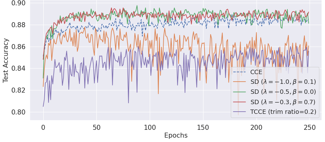
Here we provide a brief look at the convergence behavior of the proposed rSDNet with respect to the numbers of training epochs, as this directly determines the computational cost of applying robust rSDNet in practice. For this purpose, we refitted the same NN models described in Section 4 on the MNIST and Fashion-MNIST datasets, but now using their default training-test split as provided in TensorFlow. We then evaluate test accuracy for models trained over a range of epochs from 1 to 250. For both datasets, experiments were repeated for clean training data and contaminated training data with 20% and 40% uniform label noise. Additionally, for the MNIST dataset, we also considered adversarially perturbed training data generated using FGSM attacks. The resulting test accuracies are reported in Figures 5–6 for rSDNet with a few representative values of $(\beta,\lambda)\in\mathcal{T}$, alongside benchmark results obtained using the standard CCE loss and its trimmed variant TCCE(0.2).

The results show that, under clean data, rSDNet exhibits a convergence rate comparable to both CCE and TCCE(0.2), with all methods converging within a small number of epochs. However, in the presence of uniform label noise, CCE and TCCE display slower and less stable convergence, whereas rSDNet maintains a fast and stable convergence behavior similar to that observed in the clean-data scenario. Under adversarial corruption as well, rSDNet achieves convergence speeds comparable to CCE, while TCCE-based methods converge significantly more slowly. These findings demonstrate that rSDNet can be effectively applied to practical datasets, whether clean or contaminated by structured noise, without incurring additional computational cost to achieve desired level of robustness.

(a) Clean training data

(b) Contaminated training data with 20% uniform label noise

(c) Contaminated training data with 40% uniform label noise

(d) Contaminated training data under FGSM adversarial attack

Figure 5: Test accuracies obtained by different NN learning methods trained with varying numbers of epochs for the MNIST dataset

(a) Clean training data

(b) Contaminated training data with 20% uniform label noise

(c) Contaminated training data with 40% uniform label noise

Figure 6: Test accuracies obtained by different NN learning methods trained with varying numbers of epochs for the Fashion-MNIST dataset

Appendix C Tables containing empirical results

Table 1: Average $k$-fold CV accuracies of the NN classifiers trained on the three selected datasets using the proposed rSDNet with different $(\beta,\lambda)$ and the benchmark losses/classifiers under clean data [$k=7$ for MNIST and Fashion-MNIST, and $k=6$ for CIFAR-10]

Dataset $\rightarrow$	MNIST	Fashion-MNIST	CIFAR-10
Existing losses for neural classification
CCE	0.9816	0.8891	0.6782
MAE	0.9770	0.7940	0.1004
TCCE(0.1)	0.9354	0.8815	0.6733
TCCE(0.2)	0.8665	0.3094	0.6687
TCCE(0.3)	0.7787	0.2939	0.6275
rKLD	0.9643	0.8803	0.6240
SCE$(\alpha=0.5,\beta=1)$	0.9809	0.8911	0.6785
GCE$(q=0.5)$	0.9788	0.8932	0.6629
GCE$(q=0.7)$	0.9796	0.8764	0.5590
FCL$(\mu=0)$	0.9810	0.8908	0.1000
FCL$(\mu=0.25)$	0.9793	0.8898	0.6705
FCL$(\mu=0.5)$	0.1014	0.1000	0.6657
FCL$(\mu=0.75)$	0.1029	0.1007	0.5708
Proposed rSDNet, with different $(\beta,\lambda)$
$(0.05,-1)$	0.9772	0.8472	0.6457
$(0.1,-1)$	0.9782	0.8518	0.6445
$(0.3,-1)$	0.9787	0.8832	0.6617
$(0.5,-1)$	0.9780	0.8937	0.6597
$(0.7,-1)$	0.9787	0.8939	0.6585
$(0,-0.8)$	0.9789	0.8608	0.1938
$(0.05,-0.8)$	0.9782	0.8652	0.6615
$(0.1,-0.8)$	0.9791	0.8755	0.6493
$(0.3,-0.8)$	0.9786	0.8871	0.6571
$(0.5,-0.8)$	0.9797	0.8920	0.6638
$(0.7,-0.8)$	0.9789	0.8929	0.6487
$(0,-0.7)$	0.9789	0.8724	0.5653
$(0.05,-0.7)$	0.9784	0.8779	0.6625
$(0.1,-0.7)$	0.9787	0.8804	0.6623
$(0.3,-0.7)$	0.9795	0.8879	0.6464
$(0.5,-0.7)$	0.9788	0.8925	0.6561
$(0.7,-0.7)$	0.9798	0.8923	0.6563
$(0,-0.5)$	0.9796	0.8934	0.6705
$(0.05,-0.5)$	0.9806	0.8941	0.6689
$(0.1,-0.5)$	0.9801	0.8948	0.6664
$(0.3,-0.5)$	0.9801	0.8945	0.6531
$(0.5,-0.5)$	0.9801	0.8942	0.6559
$(0.7,-0.5)$	0.9782	0.8941	0.6569
$(0.1,0)$	0.9807	0.8911	0.6729
$(0.3,0)$	0.9809	0.8916	0.6670
$(0.5,0)$	0.9807	0.8937	0.6639
$(0.7,0)$	0.9798	0.8936	0.6604
$(1,0)$	0.9790	0.8933	0.6536
$(0.5,0.5)$	0.9807	0.8901	0.6626
$(0.7,0.5)$	0.9793	0.8933	0.6636

Table 2: Average 7-fold CV accuracies of the NN classifiers trained on the MNIST data using the proposed rSDNet with different $(\beta,\lambda)$ and the benchmark losses/classifiers under uniform label noise with contamination proportion $\eta$ [Highest accuracy in each case is highlighted with bold font]

$\eta\rightarrow$	0.1	0.2	0.3	0.4	0.5
Existing losses for neural classification
CCE	0.8691	0.7528	0.6461	0.5789	0.5201
MAE	0.9750	0.9720	0.9691	0.9662	0.9588
TCCE(0.1)	0.9585	0.8917	0.7654	0.6535	0.5555
TCCE(0.2)	0.9500	0.9456	0.8678	0.7448	0.6196
TCCE(0.3)	0.8764	0.9476	0.9282	0.8408	0.7057
rKLD	0.9031	0.8541	0.8123	0.7547	0.6899
SCE$(\alpha=0.5,\beta=1)$	0.8856	0.7901	0.7099	0.6373	0.5655
GCE$(q=0.5)$	0.9766	0.9715	0.9424	0.8424	0.7300
GCE$(q=0.7)$	0.9758	0.9731	0.9694	0.9629	0.9507
FCL$(\mu=0)$	0.8762	0.7593	0.6608	0.6004	0.5207
FCL$(\mu=0.25)$	0.8796	0.7718	0.6790	0.6052	0.5393
FCL$(\mu=0.50)$	0.1437	0.8215	0.7258	0.6544	0.5846
FCL$(\mu=0.75)$	0.1095	0.1063	0.1016	0.1009	0.0983
Proposed rSDNet, with different $(\beta,\lambda)$
$(0.05,-1)$	0.9742	0.9731	0.9702	0.9613	0.9544
$(0.1,-1)$	0.9753	0.9726	0.9688	0.9624	0.9407
$(0.3,-1)$	0.9752	0.9683	0.8656	0.7260	0.6165
$(0.5,-1)$	0.9746	0.8866	0.7706	0.6682	0.5922
$(0.7,-1)$	0.9613	0.8565	0.7404	0.6558	0.5906
$(1,-1)$	0.9495	0.8451	0.7469	0.6491	0.5692
$(0,-0.8)$	0.9757	0.9743	0.9681	0.9646	0.9542
$(0.05,-0.8)$	0.9760	0.9728	0.9682	0.9618	0.9451
$(0.1,-0.8)$	0.9763	0.9734	0.9683	0.9578	0.8782
$(0.3,-0.8)$	0.9753	0.9677	0.8568	0.7372	0.6200
$(0.5,-0.8)$	0.9744	0.8917	0.7789	0.6803	0.5910
$(0.7,-0.8)$	0.9659	0.8598	0.7555	0.6593	0.5842
$(0,-0.7)$	0.9772	0.9732	0.9698	0.9619	0.9503
$(0.05,-0.7)$	0.9758	0.9732	0.9668	0.9611	0.9228
$(0.1,-0.7)$	0.9774	0.9737	0.9671	0.9465	0.8092
$(0.3,-0.7)$	0.9764	0.9608	0.8556	0.7360	0.6169
$(0.5,-0.7)$	0.9735	0.8932	0.7716	0.6763	0.5909
$(0.7,-0.7)$	0.9667	0.8605	0.7560	0.6703	0.5810
$(0,-0.5)$	0.9766	0.9704	0.9433	0.8466	0.7340
$(0.1,-0.5)$	0.9755	0.9684	0.9046	0.7893	0.6667
$(0.3,-0.5)$	0.9754	0.9302	0.8153	0.7139	0.5945
$(0.5,-0.5)$	0.9730	0.8927	0.7777	0.6847	0.5825
$(0.7,-0.5)$	0.9676	0.8695	0.7577	0.6599	0.5772
$(0.1,0)$	0.8689	0.7552	0.6565	0.5876	0.5228
$(0.3,0)$	0.9021	0.7906	0.6948	0.6127	0.5333
$(0.5,0)$	0.9439	0.8410	0.7299	0.6431	0.5598
$(0.7,0)$	0.9599	0.8642	0.7589	0.6565	0.5725
$(0.5,0.5)$	0.8837	0.7670	0.6745	0.5927	0.5320
$(0.7,0.5)$	0.9397	0.8440	0.7406	0.6448	0.5573

Table 3: Average 7-fold CV accuracies of the NN classifiers trained on the Fashion-MNIST data using the proposed rSDNet with different $(\beta,\lambda)$ and the benchmark losses/classifiers under uniform label noise with contamination level $\eta$ [Highest accuracy in each case is highlighted with bold font]

$\eta\rightarrow$	0.1	0.2	0.3	0.4	0.5
Existing losses for neural classification
CCE	0.8015	0.7401	0.6955	0.6549	0.6205
MAE	0.7910	0.7907	0.7224	0.7491	0.7179
TCCE(0.1)	0.8771	0.8070	0.7387	0.6669	0.6098
TCCE(0.2)	0.8769	0.8630	0.7923	0.7137	0.6327
TCCE(0.3)	0.6118	0.8715	0.8509	0.7794	0.6848
rKLD	0.8459	0.8099	0.7711	0.7276	0.6871
SCE$(\alpha=0.5,\beta=1)$	0.8241	0.7781	0.7189	0.6772	0.6235
GCE$(q=0.5)$	0.8868	0.8816	0.8557	0.7816	0.6756
GCE$(q=0.7)$	0.8688	0.8658	0.8531	0.8604	0.8339
FCL$(\mu=0)$	0.8125	0.7513	0.7028	0.6558	0.6177
FCL$(\mu=0.25)$	0.8189	0.7514	0.6990	0.6451	0.6084
FCL$(\mu=0.50)$	0.8051	0.6845	0.7202	0.6644	0.6123
FCL$(\mu=0.75)$	0.0978	0.0990	0.0989	0.1000	0.0994
Proposed rSDNet, with different $(\beta,\lambda)$
$(0.05,-1)$	0.8581	0.8381	0.8478	0.8364	0.8259
$(0.1,-1)$	0.8565	0.8480	0.8533	0.8629	0.8405
$(0.3,-1)$	0.8865	0.8651	0.7783	0.6881	0.6301
$(0.5,-1)$	0.8757	0.7928	0.7316	0.6812	0.6535
$(0.7,-1)$	0.8678	0.7890	0.7309	0.6777	0.6372
$(0,-0.8)$	0.8615	0.8494	0.8453	0.8365	0.8316
$(0.05,-0.8)$	0.8612	0.8617	0.8427	0.8473	0.8436
$(0.1,-0.8)$	0.8684	0.8649	0.8637	0.8623	0.7924
$(0.3,-0.8)$	0.8884	0.8648	0.7719	0.6941	0.6394
$(0.5,-0.8)$	0.8798	0.8044	0.7327	0.6889	0.6381
$(0.7,-0.8)$	0.8687	0.7920	0.7237	0.6822	0.6509
$(0,-0.7)$	0.8694	0.8640	0.8353	0.8583	0.8340
$(0.05,-0.7)$	0.8706	0.8717	0.8682	0.8509	0.8304
$(0.1,-0.7)$	0.8785	0.8758	0.8745	0.8468	0.7392
$(0.3,-0.7)$	0.8883	0.8631	0.7643	0.6903	0.6466
$(0.5,-0.7)$	0.8772	0.8061	0.7335	0.6821	0.6362
$(0.7,-0.7)$	0.8721	0.7877	0.7269	0.6837	0.6385
$(0,-0.5)$	0.8888	0.8832	0.8508	0.7728	0.6851
$(0.05,-0.5)$	0.8892	0.8788	0.8359	0.7593	0.6520
$(0.1,-0.5)$	0.8873	0.8749	0.8181	0.7268	0.6205
$(0.3,-0.5)$	0.8846	0.8440	0.7469	0.6776	0.6205
$(0.5,-0.5)$	0.8825	0.8085	0.7286	0.6785	0.6438
$(0.7,-0.5)$	0.8731	0.7931	0.7346	0.6719	0.6465
$(0.1,0)$	0.8037	0.7435	0.6922	0.6534	0.6093
$(0.3,0)$	0.8283	0.7541	0.6975	0.6587	0.6162
$(0.5,0)$	0.8542	0.7785	0.7083	0.6633	0.6377
$(0.7,0)$	0.8691	0.7848	0.7247	0.6782	0.6197
$(1,0)$	0.8649	0.7979	0.7240	0.6686	0.6272
$(0.5,0.5)$	0.8138	0.7425	0.6976	0.6525	0.6042
$(0.7,0.5)$	0.8535	0.7785	0.7167	0.6630	0.6170

Table 4: Average 6-fold CV accuracies of the NN classifiers trained on the CIFAR-10 data using the proposed rSDNet with different $(\beta,\lambda)$ and the benchmark losses/classifiers under uniform label noise with contamination proportion $\eta$ [Highest accuracy in each case is highlighted with bold font]

$\eta\rightarrow$	0.1	0.2	0.3	0.4	0.5
Existing losses for neural classification
CCE	0.5884	0.5117	0.4330	0.3696	0.3004
MAE	0.0997	0.0988	0.1006	0.0987	0.0996
TCCE(0.1)	0.6440	0.5816	0.5075	0.4243	0.3425
TCCE(0.2)	0.6508	0.6137	0.5476	0.4665	0.3822
TCCE(0.3)	0.6341	0.6120	0.5576	0.4896	0.3938
rKLD	0.5445	0.4753	0.4024	0.3401	0.2695
SCE$(\alpha=0.5,\beta=1)$	0.6013	0.5314	0.4517	0.3892	0.3141
GCE$(q=0.5)$	0.6470	0.5985	0.5429	0.4680	0.3676
GCE$(q=0.7)$	0.5532	0.5299	0.5021	0.4678	0.4070
FCL$(\mu=0)$	0.1000	0.1000	0.1000	0.1000	0.1000
FCL$(\mu=0.25)$	0.6087	0.5278	0.4468	0.3744	0.3075
FCL$(\mu=0.5)$	0.6372	0.6014	0.5412	0.4539	0.3561
FCL$(\mu=0.75)$	0.4519	0.1861	0.5030	0.3904	0.4054
Proposed rSDNet, with different $(\beta,\lambda)$
$(0.05,-1)$	0.3688	0.5142	0.5066	0.5385	0.4717
$(0.1,-1)$	0.6221	0.6063	0.5712	0.5103	0.4197
$(0.3,-1)$	0.6214	0.5707	0.4995	0.4024	0.3289
$(0.5,-1)$	0.6126	0.5499	0.4674	0.3838	0.3128
$(0.7,-1)$	0.6210	0.5468	0.4567	0.3834	0.3142
$(0,-0.8)$	0.3671	0.2676	0.4258	0.3272	0.3578
$(0.05,-0.8)$	0.6323	0.6153	0.5704	0.5269	0.4476
$(0.1,-0.8)$	0.6377	0.6083	0.5642	0.4941	0.3947
$(0.3,-0.8)$	0.6253	0.5726	0.5016	0.4058	0.3259
$(0.5,-0.8)$	0.6191	0.5530	0.4678	0.3920	0.3117
$(0.7,-0.8)$	0.6138	0.5444	0.4610	0.3842	0.3074
$(0,-0.7)$	0.4519	0.5311	0.4998	0.4653	0.4631
$(0.05,-0.7)$	0.6397	0.6009	0.5639	0.5119	0.4201
$(0.1,-0.7)$	0.6368	0.6061	0.5471	0.4721	0.3804
$(0.3,-0.7)$	0.6203	0.5730	0.4863	0.4140	0.3168
$(0.5,-0.7)$	0.6240	0.5465	0.4719	0.3920	0.3066
$(0.7,-0.7)$	0.6125	0.5453	0.4691	0.3857	0.3138
$(0,-0.5)$	0.6408	0.5977	0.5342	0.4632	0.3624
$(0.05,-0.5)$	0.6375	0.5963	0.5367	0.4403	0.3544
$(0.1,-0.5)$	0.6361	0.5920	0.5207	0.4284	0.3372
$(0.3,-0.5)$	0.6270	0.5644	0.4853	0.3971	0.3127
$(0.5,-0.5)$	0.6168	0.5513	0.4689	0.3934	0.3092
$(0.7,-0.5)$	0.6151	0.5477	0.4574	0.3890	0.3164
$(0.1,0)$	0.5929	0.5128	0.4378	0.3719	0.2974
$(0.3,0)$	0.5952	0.5113	0.4483	0.3701	0.2952
$(0.5,0)$	0.6079	0.5357	0.4489	0.3759	0.3047
$(0.7,0)$	0.6172	0.5390	0.4628	0.3798	0.3093
$(1,0)$	0.6163	0.5481	0.4594	0.3853	0.3124
$(0.5,0.5)$	0.5901	0.5126	0.4338	0.3703	0.2949
$(0.7,0.5)$	0.6099	0.5366	0.4527	0.3818	0.3042

Table 5: Average test accuracies of the NN classifiers trained on adversarially perturbed MNIST images using the proposed rSDNet with different $(\beta,\lambda)$ and the benchmark losses/classifiers [Highest accuracy in each case is highlighted with bold font]

Attack type $\rightarrow$	FGSM		PGD		CW		Deepfool
	Clean test	Adv. test	Clean test	Adv. test	Clean test	Adv. test	Clean test	Adv. test
Existing losses for neural classification
CCE	0.9073	0.9776	0.6516	0.9949	0.9815	0.9815	0.9731	0.9833
MAE	0.9000	0.9744	0.6005	0.9910	0.9770	0.9770	0.9671	0.9807
TCCE(0.1)	0.7947	0.9383	0.4653	0.9870	0.9549	0.9549	0.9466	0.9574
TCCE(0.2)	0.7387	0.9117	0.4493	0.9434	0.9184	0.9184	0.9086	0.9147
TCCE(0.3)	0.6482	0.8421	0.4142	0.8823	0.8808	0.8808	0.8848	0.8733
SCE$(\alpha=0.5,\beta=1)$	0.9094	0.9765	0.6732	0.9948	0.9809	0.9809	0.9720	0.9846
GCE($q=0.5$)	0.9133	0.9730	0.5858	0.9913	0.9788	0.9788	0.9708	0.9841
GCE($q=0.7$)	0.9090	0.9745	0.5992	0.9910	0.9796	0.9796	0.9666	0.9811
FCL$(\mu=0)$	0.9156	0.9773	0.6777	0.9945	0.9810	0.9810	0.9735	0.9844
FCL$(\mu=0.25)$	0.9074	0.9733	0.6288	0.9684	0.9793	0.9793	0.9709	0.9831
FCL$(\mu=0.5)$	0.0999	0.0999	0.1012	0.1012	0.1014	0.1014	0.1016	0.1016
FCL$(\mu=0.75)$	0.1003	0.1003	0.1052	0.1052	0.1029	0.1029	0.1025	0.1025
Proposed rSDNet, with different $(\beta,\lambda)$
$(0.1,-1)$	0.9080	0.9726	0.5822	0.9957	0.9774	0.9774	0.9678	0.9821
$(0.3,-1)$	0.9083	0.9743	0.5848	0.9958	0.9793	0.9793	0.9664	0.9812
$(0.5,-1)$	0.9221	0.9749	0.6157	0.9955	0.9788	0.9788	0.9695	0.9830
$(0.7,-1)$	0.9194	0.9753	0.6174	0.9954	0.9781	0.9781	0.9674	0.9814
$(0.9,-1)$	0.9192	0.9752	0.5984	0.9954	0.9791	0.9791	0.9708	0.9835
$(0.1,-0.7)$	0.9078	0.9750	0.5879	0.9954	0.9788	0.9788	0.9691	0.9823
$(0.3,-0.7)$	0.9112	0.9738	0.5951	0.9953	0.9784	0.9784	0.9661	0.9808
$(0.5,-0.7)$	0.9141	0.9753	0.5968	0.9955	0.9790	0.9790	0.9686	0.9826
$(0.7,-0.7)$	0.9184	0.9748	0.6068	0.9953	0.9792	0.9792	0.9675	0.9817
$(0.9,-0.7)$	0.9214	0.9747	0.6004	0.9957	0.9795	0.9795	0.9683	0.9819
$(0.1,-0.5)$	0.9105	0.9749	0.5940	0.9953	0.9787	0.9787	0.9703	0.9838
$(0.3,-0.5)$	0.9122	0.9756	0.6017	0.9956	0.9796	0.9796	0.9685	0.9822
$(0.5,-0.5)$	0.9138	0.9759	0.6030	0.9952	0.9789	0.9789	0.9688	0.9825
$(0.7,-0.5)$	0.9205	0.9751	0.6081	0.9954	0.9797	0.9797	0.9683	0.9818
$(0.9,-0.5)$	0.9186	0.9753	0.6018	0.9955	0.9785	0.9785	0.9683	0.9823
$(0.1,-0.3)$	0.9099	0.9775	0.5743	0.9956	0.9797	0.9797	0.9712	0.9844
$(0.3,-0.3)$	0.9110	0.9763	0.5820	0.9954	0.9787	0.9787	0.9720	0.9847
$(0.5,-0.3)$	0.9098	0.9757	0.5796	0.9953	0.9794	0.9794	0.9706	0.9834
$(0.7,-0.3)$	0.9209	0.9749	0.5900	0.9955	0.9792	0.9792	0.9688	0.9826
$(0.9,-0.3)$	0.9143	0.9764	0.6153	0.9955	0.9789	0.9789	0.9696	0.9829
$(0.1,0)$	0.9125	0.9768	0.6265	0.9949	0.9807	0.9807	0.9730	0.9844
$(0.3,0)$	0.9124	0.9763	0.6439	0.9950	0.9808	0.9808	0.9726	0.9853
$(0.5,0)$	0.9188	0.9741	0.5982	0.9955	0.9793	0.9793	0.9713	0.9846
$(0.7,0)$	0.9108	0.9760	0.5969	0.9952	0.9787	0.9787	0.9707	0.9837
$(1,0)$	0.9160	0.9755	0.5865	0.9955	0.9788	0.9788	0.9680	0.9823
$(0.1,0.5)$	0.8725	0.9747	0.5922	0.9944	0.9702	0.9702	0.9643	0.9771
$(0.3,0.5)$	0.9076	0.9779	0.6222	0.9947	0.9809	0.9809	0.9727	0.9846
$(0.5,0.5)$	0.9116	0.9755	0.6273	0.9952	0.9809	0.9809	0.9732	0.9854
$(0.7,0.5)$	0.9123	0.9755	0.6176	0.9948	0.9805	0.9805	0.9708	0.9841
$(0.9,0.5)$	0.9235	0.9757	0.5955	0.9956	0.9785	0.9785	0.9690	0.9822

References

- Abadi et al., (2016) Abadi, M. et al. (2016). Tensorflow: A system for large-scale machine learning. https://tensorflow.org.
- Bae et al., (2022) Bae, J., Ng, N., Lo, A., Ghassemi, M., and Grosse, R. B. (2022). If influence functions are the answer, then what is the question? Advances in Neural Information Processing Systems, 35:17953–17967.
- Bartlett et al., (2006) Bartlett, P. L., Jordan, M. I., and McAuliffe, J. D. (2006). Convexity, classification, and risk bounds. Journal of the American Statistical Association, 101(473):138–156.
- Basak and Basu, (2022) Basak, S. and Basu, A. (2022). The extended bregman divergence and parametric estimation. Statistics, 56(3):699–718.
- Basu et al., (1998) Basu, A., Harris, I. R., Hjort, N. L., and Jones, M. (1998). Robust and efficient estimation by minimising a density power divergence. Biometrika, 85(3):549–559.
- Basu et al., (2011) Basu, A., Shioya, H., and Park, C. (2011). Statistical inference: the minimum distance approach. CRC press.
- Basu et al., (2021) Basu, S., Pope, P., and Feizi, S. (2021). Influence functions in deep learning are fragile. In International Conference on Learning Representations (ICLR).
- Bolte and Pauwels, (2021) Bolte, J. and Pauwels, E. (2021). Conservative set valued fields, automatic differentiation, stochastic gradient methods and deep learning. Mathematical Programming, 188(1):19–51.
- Carlini and Wagner, (2017) Carlini, N. and Wagner, D. (2017). Towards evaluating the robustness of neural networks. In 2017 ieee symposium on security and privacy (sp), pages 39–57. Ieee.
- Cichocki et al., (2011) Cichocki, A., Cruces, S., and Amari, S.-i. (2011). Generalized alpha-beta divergences and their application to robust nonnegative matrix factorization. Entropy, 13(1):134–170.
- Cohen et al., (2019) Cohen, J., Rosenfeld, E., and Kolter, Z. (2019). Certified adversarial robustness via randomized smoothing. In international conference on machine learning, pages 1310–1320. PMLR.
- Cressie and Read, (1984) Cressie, N. and Read, T. R. (1984). Multinomial goodness-of-fit tests. Journal of the Royal Statistical Society Series B: Statistical Methodology, 46(3):440–464.
- Ghosh, (2015) Ghosh, A. (2015). Asymptotic properties of minimum s-divergence estimator for discrete models. Sankhya A, 77(2):380–407.
- Ghosh and Basu, (2017) Ghosh, A. and Basu, A. (2017). The minimum s-divergence estimator under continuous models: The basu–lindsay approach. Statistical Papers, 58(2):341–372.
- (15) Ghosh, A., Harris, I. R., Maji, A., Basu, A., and Pardo, L. (2017a). A generalized divergence for statistical inference. Bernoulli, 23(4A):2746–2783.
- Ghosh and Jana, (2026) Ghosh, A. and Jana, S. (2026). Provably robust learning of regression neural networks using -divergences. arXiv preprint arXiv:2602.08933.
- (17) Ghosh, A., Kumar, H., and Sastry, P. S. (2017b). Robust loss functions under label noise for deep neural networks. In Proceedings of the AAAI conference on artificial intelligence, volume 31.
- Goodfellow et al., (2016) Goodfellow, I., Bengio, Y., and Courville, A. (2016). Deep Learning. MIT Press.
- Goodfellow et al., (2014) Goodfellow, I. J., Shlens, J., and Szegedy, C. (2014). Explaining and harnessing adversarial examples. arXiv preprint arXiv:1412.6572.
- Hampel et al., (1986) Hampel, F. R., Ronchetti, E. M., Rousseeuw, P. J., and Stahel, W. A. (1986). Robust Statistics: The Approach Based on Influence Functions. John Wiley & Sons.
- Han et al., (2018) Han, B., Yao, Q., Yu, X., Niu, G., Xu, M., Hu, W., Tsang, I., and Sugiyama, M. (2018). Co-teaching: Robust training of deep neural networks with extremely noisy labels. Advances in neural information processing systems, 31.
- Hornik et al., (1989) Hornik, K., Stinchcombe, M., and White, H. (1989). Multilayer feedforward networks are universal approximators. Neural networks, 2(5):359–366.
- Kingma and Ba, (2014) Kingma, D. P. and Ba, J. (2014). Adam: A method for stochastic optimization. arXiv preprint arXiv:1412.6980.
- Kurucu et al., (2025) Kurucu, M. C., Kumbasar, T., Eksin, İ., and Güzelkaya, M. (2025). Introducing fractional classification loss for robust learning with noisy labels. arXiv preprint arXiv:2508.06346.
- Madry et al., (2017) Madry, A., Makelov, A., Schmidt, L., Tsipras, D., and Vladu, A. (2017). Towards deep learning models resistant to adversarial attacks. arXiv preprint arXiv:1706.06083.
- Moosavi-Dezfooli et al., (2016) Moosavi-Dezfooli, S.-M., Fawzi, A., and Frossard, P. (2016). Deepfool: a simple and accurate method to fool deep neural networks. In Proceedings of the IEEE conference on computer vision and pattern recognition, pages 2574–2582.
- Natarajan et al., (2013) Natarajan, N., Dhillon, I. S., Ravikumar, P. K., and Tewari, A. (2013). Learning with noisy labels. Advances in neural information processing systems, 26.
- Patrini et al., (2017) Patrini, G., Rozza, A., Krishna Menon, A., Nock, R., and Qu, L. (2017). Making deep neural networks robust to label noise: A loss correction approach. In Proceedings of the IEEE conference on computer vision and pattern recognition, pages 1944–1952.
- Qian et al., (2022) Qian, Z., Huang, K., Wang, Q.-F., and Zhang, X.-Y. (2022). A survey of robust adversarial training in pattern recognition: Fundamental, theory, and methodologies. Pattern Recognition, 131:108889.
- Ren et al., (2018) Ren, M., Zeng, W., Yang, B., and Urtasun, R. (2018). Learning to reweight examples for robust deep learning. In International conference on machine learning, pages 4334–4343. PMLR.
- Rice et al., (2020) Rice, L., Wong, E., and Kolter, Z. (2020). Overfitting in adversarially robust deep learning. In International conference on machine learning, pages 8093–8104. PMLR.
- Roy et al., (2026) Roy, S., Sarkar, A., Ghosh, A., and Basu, A. (2026). Asymptotic breakdown point analysis for a general class of minimum divergence estimators. Bernoulli, 32(1):698–722.
- Rusiecki, (2007) Rusiecki, A. (2007). Robust lts backpropagation learning algorithm. In Computational and Ambient Intelligence: 9th International Work-Conference on Artificial Neural Networks, IWANN 2007, San Sebastián, Spain, June 20-22, 2007. Proceedings 9, pages 102–109. Springer.
- Rusiecki, (2013) Rusiecki, A. (2013). Robust learning algorithm based on lta estimator. Neurocomputing, 120:624–632.
- Rusiecki, (2019) Rusiecki, A. (2019). Trimmed categorical cross-entropy for deep learning with label noise. Electronics Letters, 55(6):319–320.
- Rusiecki, (2020) Rusiecki, A. (2020). Standard dropout as remedy for training deep neural networks with label noise. In International Conference on Dependability and Complex Systems, pages 534–542. Springer.
- Sinha et al., (2018) Sinha, A., Namkoong, H., and Duchi, J. (2018). Certifying some distributional robustness with principled adversarial training. In International Conference on Learning Representations.
- Song et al., (2022) Song, H., Kim, M., Park, D., Shin, Y., and Lee, J.-G. (2022). Learning from noisy labels with deep neural networks: A survey. IEEE transactions on neural networks and learning systems, 34(11):8135–8153.
- Srivastava et al., (2014) Srivastava, N., Hinton, G., Krizhevsky, A., Sutskever, I., and Salakhutdinov, R. (2014). Dropout: a simple way to prevent neural networks from overfitting. The journal of machine learning research, 15(1):1929–1958.
- Szegedy et al., (2013) Szegedy, C., Zaremba, W., Sutskever, I., Bruna, J., Erhan, D., Goodfellow, I., and Fergus, R. (2013). Intriguing properties of neural networks. arXiv preprint arXiv:1312.6199.
- Tewari and Bartlett, (2007) Tewari, A. and Bartlett, P. L. (2007). On the consistency of multiclass classification methods. Journal of Machine Learning Research, 8(5).
- Wang et al., (2019) Wang, Y., Ma, X., Chen, Z., Luo, Y., Yi, J., and Bailey, J. (2019). Symmetric cross entropy for robust learning with noisy labels. In Proceedings of the IEEE/CVF international conference on computer vision, pages 322–330.
- Zhang et al., (2017) Zhang, C., Bengio, S., Hardt, M., Recht, B., and Vinyals, O. (2017). Understanding deep learning requires rethinking generalization. In International Conference on Learning Representations.
- Zhang et al., (2019) Zhang, H., Yu, Y., Jiao, J., Xing, E., El Ghaoui, L., and Jordan, M. (2019). Theoretically principled trade-off between robustness and accuracy. In International conference on machine learning, pages 7472–7482. PMLR.
- Zhang, (2004) Zhang, T. (2004). Statistical behavior and consistency of classification methods based on convex risk minimization. The Annals of Statistics, 32(1):56–85.
- Zhang and Sabuncu, (2018) Zhang, Z. and Sabuncu, M. (2018). Generalized cross entropy loss for training deep neural networks with noisy labels. Advances in neural information processing systems, 31.