Translation Invariance of Neural Operators for the FitzHugh–Nagumo Model

Abstract

Neural Operators (NOs) are a powerful deep learning framework designed to learn the solution operator that arise from partial differential equations. This study investigates NOs ability to capture the stiff spatio-temporal dynamics of the FitzHugh-Nagumo model, which describes excitable cells. A key contribution of this work is evaluating the translation invariance using a novel training strategy. NOs are trained using an applied current with varying spatial locations and intensities at a fixed time, and the test set introduces a more challenging out-of-distribution scenario in which the applied current is translated in both time and space. This approach significantly reduces the computational cost of dataset generation. Moreover we benchmark seven NOs architectures: Convolutional Neural Operators (CNOs), Deep Operator Networks (DONs), DONs with CNN encoder (DONs-CNN), Proper Orthogonal Decomposition DONs (POD-DONs), Fourier Neural Operators (FNOs), Tucker Tensorized FNOs (TFNOs), Localized Neural Operators (LocalNOs). We evaluated these models based on training and test accuracy, efficiency, and inference speed. Our results reveal that CNOs performs well on translated test dynamics. However, they require higher training costs, though their performance on the training set is similar to that of the other considered architectures. In contrast, FNOs achieve the lowest training error, but have the highest inference time. Regarding the translated dynamics, FNOs and their variants provide less accurate predictions. Finally, DONs and their variants demonstrate high efficiency in both training and inference, however they do not generalize well to the test set. These findings highlight the current capabilities and limitations of NOs in capturing complex ionic model dynamics and provide a comprehensive benchmark including their application to scenarios involving translated dynamics.

Keywords: Neural Operators, FitzHugh-Nagumo model, stiff PDEs, computational electrophysiology

 

 

1 Introduction

The FitzHugh-Nagumo (FHN) model [7] is widely used in computational electrophysiology [4, 14], with significant applications in both computational neuroscience [13] and computational cardiology [6]. Originally derived as a simplification of the biophysically detailed Hodgkin-Huxley model [11], the FHN system accurately captures the essential dynamics of action potential propagation while significantly reducing computational cost. This balance between physical fidelity and efficiency is the reason why the model remains so widely used today [4]. Mathematically, the system is characterized by a parabolic reaction-diffusion partial differential equation (PDE) coupled with a stiff ordinary differential equation (ODE). In recent years, there has been significant interest in applying Scientific Machine Learning (SciML) techniques to computational electrophysiology [5, 8, 12, 26, 29, 30, 32], that aim to exploit the non-linear approximation capabilities of Artificial Neural Networks (ANNs) to solve both forward and inverse problems. Among the many ANN-based methods, Neural Operators (NOs) [16] represent a paradigm shift. These architectures are designed to learn mappings between infinite-dimensional function spaces. While numerous NOs architectures have been proposed in recent years, a comprehensive comparison of every available variant is practically unfeasible. In particular, we consider the following: Convolutional Neural Operators (CNOs) [27], Deep Operator Networks (DONs) [23] including variants such as DONs with CNN encoders (DONs-CNN) [16] and Proper Orthogonal Decomposition DON (POD-DONs) [24] Fourier Neural Operators (FNOs) [20] and the following variants Tucker Tensorized Fourier Neural Operators (TFNOs) [31], and Localized Neural Operators (LocalNOs) [22]. The aim of this work is to provide a comprehensive and rigorous comparison by evaluating the accuracy in both train and test set, as well as the associated computational costs (training and inference). Furthermore, we exploit a fundamental physical property of the FHN model, which we will refer to as translation invariance. Given a constant set of parameters, the solution with respect to an applied current remains invariant regardless of its translation in time. We investigate whether NOs can intrinsically capture this property. Consequently, we propose a novel training strategy in which the training dataset is generated with an applied current that varies in spatial position and intensity while remaining fixed in time, while the test set introduces a more challenging out-of-distribution scenario in which the applied current is translated in both time and space. This approach enables us to assess which architectures effectively learn the underlying invariance property, which could help to reduce the computational burden of generating large-scale datasets.

The paper is organized as follows: Section 2 defines the mathematical formulation of the FHN model and the novel training strategy that exploits translation invariance. Furthermore, we provide a formal introduction to NOs and to the specific architectures considered (CNOs, DONs, DONs-CNN, POD-DONs, FNOs, TFNOs, and LocalNOs). Section 3 presents the numerical results obtained for each architecture. Section 4 provides an in-depth comparison of the models based on accuracy, computational efficiency, inference speed, and cost functions that will be introduced that take into account accuracy, training time, and the number of trainable parameters. Finally, Section 5 summarizes our findings, and outlines directions for future research.

2 Mathematical models and methods

The FHN model is described by a coupled system of a parabolic reaction-diffusion PDE for the transmembrane potential $\displaystyle V$ and a stiff ODE for the gating variable $\displaystyle w$.

$$\begin{cases}\chi C_{m}\frac{\partial V}{\partial t}-\text{div}(D(x)\nabla V)+\chi I_{ion}(V,w)=I_{app},\quad&\text{in }\Omega_{T}\\ \frac{\partial w}{\partial t}-R(V,w)=0,\quad&\text{in }\Omega_{T}\\ \textbf{n}^{T}D_{m}\nabla V=0,\quad&\text{on }\Gamma_{T}\\ V(x,0)=V_{0}(x),\quad w(x,0)=w_{0}(x),\quad&\text{in }\Omega\end{cases}$$ (1)

where $\displaystyle\Omega_{T}=\Omega\times(0,T]$. A more detailed description of the model is provided in Appendix A.1. Throughout this work, we focus on the operator that maps the applied current $\displaystyle I_{app}$ to the solution $\displaystyle(V,w)$:

$$\displaystyle\mathcal{G}^{\dagger}:\mathcal{A} \displaystyle\rightarrow\mathcal{D}$$ (2)

$$\displaystyle I_{app} \displaystyle\mapsto(V,w)$$

where the applied current is defined as a piecewise constant function:

$$I_{app}(i,x,t)=\begin{cases}i,\ \ (x,t)\in\Omega_{T,stim}\\ 0,\ \ (x,t)\notin\Omega_{T,stim}\end{cases}$$ (3)

Here, $\displaystyle\Omega_{T,stim}=\Omega_{stim}\times[T_{min},T_{max}]$, where $\displaystyle\Omega_{stim}\subset\Omega$ represents the region affected by the stimulus. As previously underlined, the FHN model exhibits a property that we refer as: translation invariance. This implies that, for a fixed set of parameters for the FHN model (1), stimulus intensity $\displaystyle i$, and spatial position $\displaystyle\Omega_{stim}$, shifting the stimulus with respect to time results in an identical solution that has merely translated in time. This behaviour is illustrated in Figure 1.

Figure 1: Example of translation invariance of the FHN model. Each column shows the evolution of the voltage V (second row) and the recovery variable w (third row) in response to an applied current $\displaystyle I_{app}$ (3) (first row), with an intensity of $\displaystyle i=3$, a duration of 1 ms, and spatial width 0.04 at 0.5. The stimulus $\displaystyle I_{app}$ is applied at three different times: 5 ms (first column), 35 ms (second column), and 25 ms (third column). These results were obtained using the Firedrake finite element library [10].

Our objective is to leverage this invariance by generating a training set in which the stimulus intensity $\displaystyle i$ and the spatial position $\displaystyle\Omega_{stim}$ are varied, while keeping the stimulus time ($\displaystyle T_{min}$ and $\displaystyle T_{max}$) fixed. This strategy is depicted in Figure 2.

Figure 2: Examples from the training dataset for the FHN model. Each column illustrates the evolution of the voltage V (second row) and the recovery variable w (third row) in response to an applied current $\displaystyle I_{app}$ (3) (first row). In particular, the first column has an intensity $\displaystyle i=3$ at position 0.1, the second column has intensity of $\displaystyle i=0.5$ at position 0.5, and the third column has an intensity of $\displaystyle i=1.5$ at position 0.7. The stimulus begins at the same time for all three examples and has the same duration and spatial width: 5 ms, 1 ms, and 0.04, respectively. These results were obtained using the Firedrake finite element library [10].

While, for the test and validation datasets, we vary the stimulus intensity $\displaystyle i$ and the spatial-temporal position $\displaystyle\Omega_{T,stim}$ (see Figure 3).

Figure 3: Examples from the test and validation datasets for the FHN model. Each column illustrates the evolution of the voltage V (second row) and the recovery variable w (third row) in response to an applied current $\displaystyle I_{app}$ (3) (first row). In particular, the first column has an intensity $\displaystyle i=0.1$ at $\displaystyle t=32$ ms and position $\displaystyle 0.25$; the second column has an intensity $\displaystyle i=0.5$ at $\displaystyle t=2$ ms and position $\displaystyle 0.5$; and the third column has an intensity $\displaystyle i=1.5$ at $\displaystyle t=20$ ms and position $\displaystyle 0.7$. For all three cases, the stimulus duration and spatial width are held constant at 1 ms and 0.04, respectively. These results were obtained using the Firedrake finite element library [10].

This approach significantly reduces the computational cost of generating data by eliminating the need to sample the stimulus at different times. In this study, we evaluate the capacity of several NOs architectures to learn the translation invariance property. More details about the dataset generation can be found in the Appendix A.2.

2.1 Neural Operators

NOs have emerged as a promising framework for learning mappings between infinite-dimensional function spaces, making them particularly well-suited for solving PDEs [17]. Unlike traditional neural networks, which operate on finite-dimensional spaces, NOs can learn continuous operators that map between function spaces. This section introduces NOs following the formalism presented in [1, 17], for the FHN model (1). In particular, we can rewrite our system Eq. (1) as follows:

$$\begin{cases}\mathcal{M}V\,(I_{app},V,w;x,t)=0,\quad&(x,t)\in\Omega_{T}\\ \mathcal{N}w\,(V,w;x,t)=0,\quad&(x,t)\in\Omega_{T}\\ \text{Boundary and Initial conditions.}\end{cases}$$

As previously mentioned, we are interested in the mapping defined by Eq. (2). Despite the fact that the applied current is explicitly present only in the first equation, it has an effect on both variables due to the coupled nature of the model. Therefore, the solution operator is defined as $\displaystyle\mathcal{G}^{\dagger}=\Phi^{-1}_{I_{app}}$ where $\displaystyle\Phi_{I_{app}}:=(\mathcal{M},\mathcal{N})$. Furthermore, it is essential to emphasize that the two operators, denoted by $\displaystyle\mathcal{M}$ and $\displaystyle\mathcal{N}$, exhibit distinct scales and dynamics, which makes the learning the dynamics of stiff ionic models, with NOs particularly challenging [5, 26]. In general, NOs can be expressed as a composition of different operators:

$$\mathcal{G}_{\theta}:=\mathcal{Q}\circ\mathcal{L}_{L}\circ\cdots\circ\mathcal{L}_{1}\circ\mathcal{P}:\ (I_{app},\theta)\mapsto\ (V,w)$$ (4)

where the three main components are:

• A lifting operator $\displaystyle\mathcal{P}$ which maps the input function (i.e. the applied current $\displaystyle I_{app}$) to a higher-dimensional space. This operator is typically implemented either as a shallow pointwise Multilayer Perceptron (MLP) or a single linear layer.

• A composition of integral operators $\displaystyle\mathcal{L}_{\ell}$ processing the lifted representation through $\displaystyle L$ layers in order to capture global dependencies and interactions in the input function through a sequence of transformations. Each $\displaystyle\mathcal{L}_{\ell}$ has the following structure:

  $$\mathcal{L}_{\ell}(v)(y):=\sigma\Big(W_{\ell}v(x)+b_{\ell}+\mathcal{K}_{\ell}(\theta_{\ell})v(y)\Big)$$ (5)

  where $\displaystyle v$ is the output of the previous layer, $\displaystyle W_{\ell}$ is a matrix, $\displaystyle b_{\ell}$ is a vector, $\displaystyle\theta_{\ell}\in\Theta_{\ell}\subset\Theta$ is a subset of the trainable parameters, and $\displaystyle\sigma$ is a non-linear activation function. Finally, $\displaystyle\mathcal{K}_{\ell}(\theta_{\ell})$ is a trainable linear operator.

• A projection operator $\displaystyle\mathcal{Q}$ which maps the internal representation back to the output space. This operator is also implemented as a pointwise MLP.

For a more thorough description of the mathematical properties of NOs, the reader is referred to [2, 18]. In the following sections we will give a brief introduction to the NOs architecture that will be taken into consideration thought this work (i.e. CNOs, DONs, DONs-CNN, POD-DONs, FNOs, TFNOs, and LocalNOs).

2.1.1 Convolutional Neural Operators

CNOs [27] are a modification of Convolutional Neural Networks (CNNs) designed to enforce the structure-preserving continuous equivalence and ensure the architecture is a representation-equivalent neural operator [17], which are fundamental aspects of NOs. While a detailed derivation is beyond the scope of this work, we outline the essential components here, a complete technical definition is reported in [27]. The mathematical foundation of CNOs is built upon the space of bandlimited functions, which are defined as follows:

$$\mathcal{B}_{\omega}(D,\mathbb{R}^{d_{v}})\coloneqq\{f\in L^{2}(D,\mathbb{R}^{d_{v}}:\text{supp}[\mathcal{F}(f)]\subset[-\omega,\omega]^{2})\}.$$

Where, $\displaystyle\mathcal{F}$ is the Fourier transform and $\displaystyle\omega>0$ is the bandlimit frequency. The integral operator Eq. 5 in the case of CNO is defined as follows:

$$v_{\ell+1}=\mathcal{L}_{\ell}(v_{\ell})\coloneqq\mathcal{P}_{\ell}\circ\Sigma_{\ell}\circ\mathcal{K}_{\ell}(v_{\ell}).$$

Here, $\displaystyle\mathcal{P}_{\ell}$ is either the upsampling or downsampling operator, $\displaystyle\mathcal{K}_{\ell}$ is the convolution operator and $\displaystyle\Sigma_{\ell}$ is the activation operator. Following this, we will give a brief overview of the CNO’s components, for more details refer to [9, 27].

• Upsampling $\displaystyle\mathcal{U}_{\omega,\bar{\omega}}$: This operator takes a function $\displaystyle f\in\mathcal{B}_{\omega}(D,\mathbb{R})$ and upsamples it to a higher bandlimit frequency space $\displaystyle\mathcal{B}_{\bar{\omega}}(D,\mathbb{R})$, where $\displaystyle\bar{\omega}>\omega$. Since $\displaystyle\mathcal{B}_{\omega}(D,\mathbb{R})\subset\mathcal{B}_{\bar{\omega}}(D,\mathbb{R})$ , the operation is simply the identity:

  $$\mathcal{U}_{\omega,\bar{\omega}}f(x)=f(x),\quad\forall x\in D.$$

• Downsampling $\displaystyle\mathcal{D}_{\omega,\underline{\omega}}$: This operator takes a function $\displaystyle f\in\mathcal{B}_{\omega}(D,\mathbb{R})$ and downsamples it to a lower bandlimit frequency space $\displaystyle\mathcal{B}_{\underline{\omega}}(D,\mathbb{R})$, where $\displaystyle\omega>\underline{\omega}$. It is defined as follows:

  $$\mathcal{D}_{\omega,\underline{\omega}}f(x)=\Big(\frac{\underline{\omega}}{\omega}\Big)^{2}(h_{\underline{\omega}}*f)(x).$$

  Where, $\displaystyle h_{\underline{\omega}}$ is the sinc filter defined as:

  $$h_{\omega}(x)=\prod_{i=1}^{d}\frac{sin(2\pi\omega x_{i})}{2\pi\omega x_{i}},\quad\forall x\in\mathbb{R}^{d}.$$

• Activation operator $\displaystyle\Sigma_{\omega}$: This operator is designed such that it maps functions from a bandlimited space $\displaystyle\mathcal{B}_{\omega}(D,\mathbb{R})$ back to the same space (i.e., if $\displaystyle f\in\mathcal{B}_{\omega}(D,\mathbb{R})\text{ then }\Sigma_{\omega}(f)\in\mathcal{B}_{\omega}(D,\mathbb{R}$)). It is defined as:

  $$\Sigma_{\omega}f(x)=(\mathcal{D}_{\bar{\omega},\omega}\circ\sigma\circ\mathcal{U}_{\omega,\bar{\omega}}f)(x),\quad\forall x\in D$$

  Where, $\displaystyle\sigma$ is an activation function, and $\displaystyle\bar{\omega}$ is chosen large enough such that $\displaystyle\sigma(\mathcal{B}_{\omega}(D,\mathbb{R}))\subset\mathcal{B}_{\bar{\omega}}(D,\mathbb{R})$

• Convolution Operator $\displaystyle\mathcal{K}_{\ell}$: With a slight abuse of notation, we denote $\displaystyle\mathcal{K}_{\ell}$ as $\displaystyle\mathcal{K}_{\omega,\theta}$, where $\displaystyle\omega$ is the bandwidth and $\displaystyle\theta$ are the learnable parameters. We assume there is a function $\displaystyle\kappa_{\omega,\theta}$ called the kernel function, such that the operator can be rewritten as the following convolution:

  $$\mathcal{K}_{\omega,\theta}f(x)=(f*\kappa_{\omega,\theta})(x)=\int_{D}\kappa_{\omega,\theta}(y)f(x-y)dy,\quad f\in\mathcal{B}_{\omega}(D,\mathbb{R}^{d_{v}}),\quad\forall x\in D.$$

  The integral can then be approximated as:

  $$\mathcal{K}_{\omega,\theta}f(x)\approx\sum_{i,j=1}^{k}\kappa_{\omega,\theta}(y_{ij})f(x-y_{ij})\quad\forall x\in D.$$

  Where in this context, $\displaystyle k$ is the kernel size of the convolution and $\displaystyle d_{v}$ is the channel dimension.

If we are dealing with a vector-valued function $\displaystyle f\in\mathcal{B}_{\omega}(D,\mathbb{R}^{d_{v}})$, the operators are applied component-wise. The aforementioned operators are then assembled into a U-Net architecture [28] featuring skip connection, the two additional operators described below.

• Skip Connection (ResNet Blocks) $\displaystyle\mathcal{R}_{\omega,\theta}$: These blocks connect the encoder and decoder layers at the same spatial resolution. They are useful for transferring high-frequency information to the output before it is filtered by the downsampling operation. The block is defined as:

  $$\mathcal{R}_{\omega,\theta}(v)=v+\mathcal{K}_{\omega,\theta}\circ\Sigma_{\omega}\circ\mathcal{K}_{\omega,\theta}(v),\quad\forall v\in\mathcal{B}_{\omega}(D,\mathbb{R}^{d_{v}}).$$

  The output of the residual block is concatenated with the input of the corresponding decoder block.

• Invariant Blocks $\displaystyle\mathcal{I}_{\omega,\theta}$: At every layer of the U-Net, after the concatenation of the residual block output with the decoder input, we apply an invariant block, defined as:

  $$\mathcal{I}_{\omega,\theta}=\Sigma_{\omega}\circ\mathcal{K}_{\omega,\theta}(v),\quad\forall v\in\mathcal{B}_{\omega}(D,\mathbb{R}^{d_{v}})$$

A visual representation of the CNO architecture is shown in Fig 4.

Figure 4: Visual representation of a Convolutional Neural Operator with channel multiplier $\displaystyle C$ and initial resolution equal to $\displaystyle 64$ with four layers.

2.1.2 Deep Operator Networks

DONs [23] were among the first architectures proposed to learn the infinite-dimensional mappings arising from PDEs. However, it is important to observe that their vanilla formulation does not strictly correspond to the iterative structure defined by Eq. (4). But as demonstrated in the recent study [16], under certain assumptions, DONs can be mathematically defined as NOs. In terms of architecture, a DON is defined as two sub-networks: the branch and the trunk. The branch takes as input the $\displaystyle I_{app}$ and outputs a set of coefficients, $\displaystyle[b_{1},...,b_{p}]$, where $\displaystyle p$ denotes the number of basis functions. The trunk takes the spatio-temporal coordinates, $\displaystyle(x,t)$ as input and has outputs the basis functions [$\displaystyle T_{1},...T_{p}$]. The final output is obtained by merging these two components via a dot product.

$$\mathcal{G}_{\theta}(I_{app})(x,t)=\sum_{i=1}^{p}b_{i}(I_{app})T_{i}(x,t),\quad\forall(x,t)\in\Omega_{T}.$$

Here, $\displaystyle\theta$ represents the trainable parameters of both the branch and trunk networks. To handle the coupled system of PDEs, one could potentially employ two separate DONs architectures and optimize them through a joint loss function. In this work, however, we employ a single DONs and split the output into two components. In particular, for a total of $\displaystyle p$ basis, we employ $\displaystyle p/2$ basis and their corresponding coefficients for the potential $\displaystyle V$, and the remaining $\displaystyle p/2$ for the gating variable $\displaystyle w$. This can be written as:

$$\mathcal{G}_{\theta}(I_{app})(x,t)=\underbrace{\sum_{i=1}^{p/2}b_{i}(I_{app})T_{i}(x,t)}_{V_{\theta}}+\underbrace{\sum_{i=p/2+1}^{p}b_{i}(I_{app})T_{i}(x,t)}_{w_{\theta}},\quad\forall(x,t)\in\Omega_{T}.$$

We adopted this single-architecture approach based on the idea that a unified network should capture the ionic model’s intrinsic cross-dependencies and coupled dynamics. A visual representation of this architecture is shown in Fig. 5.

Figure 5: Visual representation of a DON architecture.

Moreover, we will consider the following modification of the DON:

• DONs with CNN encoders (DONs-CNN): In this variant, the input of the branch $\displaystyle I_{app}$ is not given directly to a fully connected ANN, but Instead, but instead first passes through a series of convolutional layers.

• Proper Orthogonal Decomposition DONs (POD-DONs) [24]: This architecture combines the operator learning capabilities of DONs with the dimensionality reduction technique POD. Rather than using an ANN for the trunk network, the output is a linear combination of POD modes extracted from the training data.

2.1.3 Fourier Neural Operators

FNOs [17, 20] are a class of NOs that employs the Fourier transform to efficiently parameterize the integral kernel operator $\displaystyle\mathcal{K}_{\ell}(\theta_{\ell})$ Eq. (5). By operating in the frequency domain, FNOs effectively capture global dependencies within input functions. In the case of FNOs, the integral kernel operator is defined as follows:

$$\mathcal{K}_{\ell,\theta_{\ell}}v(y)=\int_{\mathbb{T}^{d}}\kappa_{\ell,\theta_{\ell}}(y,s)v(s)\ ds=\int_{\mathbb{T}^{d}}\kappa_{\ell,\theta_{\ell}}(y-s)v(s)\ ds=(\kappa_{\ell,\theta_{\ell}}*v)(y)$$ (6)

where $\displaystyle\mathbb{T}^{d}$ is the $\displaystyle d$-dimensional torus, and $\displaystyle\kappa_{\ell,\theta_{\ell}}$ is a kernel function, which depends on the learnable parameters $\displaystyle\theta_{\ell}$. We can apply the convolution theorem for the Fourier transform in order to rewrite the convolution in (6) in the Fourier domain:

$$(\kappa_{\ell,\theta_{\ell}}*v)(y)=\mathcal{F}^{-1}\left(\mathcal{F}(\kappa_{\ell,\theta_{\ell}})(k)\cdot\mathcal{F}(v)(k)\right)(y).$$

The key step in FNOs is the parameterization of $\displaystyle\mathcal{F}(\kappa_{\ell,\theta_{\ell}})(k)$ using a complex-valued matrix of learnable parameters $\displaystyle R_{\theta_{\ell}}(k)\in\mathbb{C}^{d_{v}\times d_{v}}$ for each frequency mode $\displaystyle k\in\mathbb{Z}^{d}$, obtaining:

$$(\mathcal{K}_{\ell,\theta_{\ell}}v)(y)=\mathcal{F}^{-1}\left(R_{\theta_{\ell}}(k)\cdot\mathcal{F}(v)(k)\right)(y).$$

Since we consider real-valued functions, the parameterized matrix $\displaystyle R_{\theta_{\ell}}(k)$ must be Hermitian, i.e., $\displaystyle R_{\theta_{\ell}}(-k)=\overline{R_{\theta_{\ell}}(k)}$ for all $\displaystyle k\in\mathbb{Z}^{d}$ and $\displaystyle\ell=1,\ldots,L$. Furthermore, in order to apply the Fast Fourier Transform (FFT) for the numerical implementation of the Fourier transform, the mesh considered must be structured and uniform.

Figure 6: Visual representation of a FNO.

In our implementation, we have considered two versions of (5):

$$\displaystyle v_{\ell+1}^{Classic} \displaystyle=\mathcal{L}_{\ell}^{Classic}(v_{\ell}):=\sigma\Big(W_{\ell}v_{\ell}+b_{\ell}+\mathcal{K}_{\ell,\theta_{\ell}}v_{\ell}\Big),$$ (7)

$$\displaystyle v_{\ell+1}^{MLP} \displaystyle=\mathcal{L}_{\ell}^{MLP}(v_{\ell}):=\sigma\Big(W_{\ell}v_{\ell}+b_{\ell}+MLP(\mathcal{K}_{\ell,\theta_{\ell}}v_{\ell})\Big),$$ (8)

where $\displaystyle v_{\ell+1}^{\text{Classic}}$ has the exact structure described in (5), while $\displaystyle v_{\ell+1}^{\text{MLP}}$ generalizes the classic architecture by incorporating a pointwise MLP applied to the output of the integral kernel operator. Moreover, we will consider two modifications of the FNOs:

• Local Neural Operators (LocalNOs) [22]: It employs localized integral kernels to capture high-frequency local features and discontinuities.

• Tucker Tensorized FNOs (TFNOs) [31]: It combines Tucker tensor decomposition with FNOs by applying tensor decomposition to the Fourier weights, significantly reducing the model memory requirement and computational cost in high-dimensional spaces.

3 Numerical Results

In this section, we present the results of the numerical tests performed. We employed HyperNOs [9] a PyTorch library, which implements automatic hyperparameter tuning of NOs based on Ray [21]. All tests were performed on a Linux cluster. Two nodes, each with two NVIDIA A16 GPUs, were used for the automatic hyperparameter tuning. For single training, we used one node with an NVIDIA A16 GPU. For inference time, we used a laptop with an NVIDIA GeForce RTX 4070 GPU. More details about automatic hyperparameter tuning are reported in Appendix B. In the following Table 1 we reports the results obtained by the different architectures in terms of the number of trainable parameters, training time, training error and test error. The training time is reported as both the total time required for training and the average time per epoch. Training and test errors are reported in terms of $\displaystyle L^{2}$ and $\displaystyle L^{1}$ relative norms, with respective means and standard deviations across five runs with different random seeds. A more detailed comparison of the results obtained by the different architectures is discussed in Section 4.

Architecture	Number of	Training Time		Training Error	Test
	parameters	Total	Epoch	$\displaystyle L^{2}$	$\displaystyle L^{2}$		$\displaystyle L^{1}$
					Mean	Median	Mean	Median
CNO	8.2 M	10 h	36.4 sec	$\displaystyle 0.0323\pm 0.0059$	$\displaystyle 0.1501\pm 0.0443$	$\displaystyle 0.0985\pm 0.0152$	$\displaystyle 0.0941\pm 0.0332$	$\displaystyle 0.0535\pm 0.0123$
DON	1.5M	30m	1.73 sec	$\displaystyle 0.0273\pm 0.0041$	$\displaystyle 0.7190\pm 0.0380$	$\displaystyle 0.8161\pm 0.0001$	$\displaystyle 0.5756\pm 0.0536$	$\displaystyle 0.6532\pm 0.0132$
DON-CNN	0.5M	15 min	0.88 sec	$\displaystyle 0.1701\pm 0.0066$	$\displaystyle 0.6861\pm 0.0068$	$\displaystyle 0.7772\pm 0.0178$	$\displaystyle 0.6008\pm 0.0155$	$\displaystyle 0.6559\pm 0.0241$
POD-DON	1M	16m	0.98 sec	$\displaystyle 0.0439\pm 0.0012$	$\displaystyle 0.6953\pm 0.0007$	$\displaystyle 0.8146\pm 0.0009$	$\displaystyle 0.5535\pm 0.0028$	$\displaystyle 0.6497\pm 0.0010$
FNO	151.1 M	4 h	15.8 sec	$\displaystyle 0.0081\pm 0.0003$	$\displaystyle 1.0333\pm 0.6000$	$\displaystyle 0.5393\pm 0.1218$	$\displaystyle 1.4655\pm 1.0330$	$\displaystyle 0.4894\pm 0.1041$
LocalNO	0.15 M	1h	4.91 sec	$\displaystyle 0.0423\pm 0.0121$	$\displaystyle 2.8717\pm 2.3716$	$\displaystyle 1.4850\pm 1.4840$	$\displaystyle 4.2232\pm 3.5578$	$\displaystyle 1.5667\pm 1.6579$
TFNO	0.3 M	9h	35.95 sec	$\displaystyle 0.0444\pm 0.0067$	$\displaystyle 0.9378\pm 0.1813$	$\displaystyle 0.4378\pm 0.1259$	$\displaystyle 1.5174\pm 0.4191$	$\displaystyle 0.4070\pm 0.0905$

Table 1: Summary of the results obtained by the different architecture.

In the following sections, we will provide a detailed description of the results obtained by each architecture. Each architecture has been trained using AdamW with weight decay regularization $\displaystyle\omega$ for 1000 epochs. We also use a learning rate scheduler that decreases the learning rate $\displaystyle\eta$ by a factor of $\displaystyle\gamma$ every ten epochs. The dataset has 2000 examples for training and 500 for the test, more details are in the Appendix A.2.

3.1 Convolutional Neural Operators results

The hyperparameters that are employed for the CNO [27], as well as the range considered for the automatic hyperparameter tuning, are listed in the Appendix B.1 in particular, in Table 4. Figure 7 shows the evolution of relative $\displaystyle L^{2}$ training loss and relative $\displaystyle L^{1}$ and $\displaystyle L^{2}$ test losses, averaged over five random seeds (Fig. 7(a)), as well as the bar plots illustrating the distribution of errors for the training and test sets (Fig. 7(b)).

(a) Loss values for the CNO.

(b) Bar plot for the CNO.

Figure 7: CNO performance metrics: (a) Evolution of the relative $\displaystyle L^{2}$ training loss (blue), relative $\displaystyle L^{1}$ test loss (green), and relative $\displaystyle L^{2}$ test loss (red) across epochs. (b) Distribution of the relative $\displaystyle L^{2}$ error for the training and test sets.

From the error distribution in Figure 7(b), we can observe that CNO performs well in the training with a relative $\displaystyle L^{2}$ error around $\displaystyle 10^{-2}$. However, there are some outliers. Concerning the test set, we observe that we have higher errors. Even considering this, we see that CNOs can capture the translation invariance of the FHN model with slightly less accuracy. Figure 8 shows four randomly selected examples from the training and test sets to visualize the results.

Figure 8: CNO visualization: Four randomly selected examples from the training and test sets are shown. Within each column, the rows illustrate: the applied current $\displaystyle I_{\text{app}}$, high-fidelity reference for potential $\displaystyle V$, CNO prediction $\displaystyle V_{\theta}$ for $\displaystyle V$, pointwise error for $\displaystyle V$, high-fidelity reference for recovery variable $\displaystyle w$, CNO prediction $\displaystyle w_{\theta}$ for $\displaystyle w$, pointwise error $\displaystyle w$.

3.2 Deep Operator Networks results

We report the results obtained for the DON [23] without any modification, i.e., both the branch and the trunk are feed-forward neural networks (FNNs). The hyperparameters that are employed and the range considered for the automatic hyperparameter tuning, are listed in the Appendix B.2 in particular, in Table 5. Figure 9 shows the evolution of relative $\displaystyle L^{2}$ training loss and relative $\displaystyle L^{1}$ and $\displaystyle L^{2}$ test losses, averaged over five random seeds (Fig. 9(a)), as well as the bar plots illustrating the distribution of errors for the training and test sets (Fig. 9(b)).

(a) Loss values for the DONs.

(b) Bar plot for the DONs.

Figure 9: DON performance metrics: (a) Evolution of the relative $\displaystyle L^{2}$ training loss (blue), relative $\displaystyle L^{1}$ test loss (green), and relative $\displaystyle L^{2}$ test loss (red) across epochs. (b) Distribution of the relative $\displaystyle L^{2}$ error for the training and test sets.

From the error distribution in Figure 9(b), we can observe that DON performs well in the training with a relative $\displaystyle L^{2}$ error around $\displaystyle 10^{-2}$. However, when it comes to the test set, we see that DONs face challenges replicating the FHN translation invariance property. To further highlight this, we visualize the results, Figure 10 shows four randomly selected examples from the training and test sets to visualize the results.

Figure 10: DON visualization: Four randomly selected examples from the training and test sets are shown. Within each column, the rows illustrate: the applied current $\displaystyle I_{\text{app}}$, high-fidelity reference for potential $\displaystyle V$, DON prediction $\displaystyle V_{\theta}$ for $\displaystyle V$, pointwise error for $\displaystyle V$, high-fidelity reference for recovery variable $\displaystyle w$, DON prediction $\displaystyle w_{\theta}$ for $\displaystyle w$, pointwise error $\displaystyle w$.

3.3 Deep Operator Networks with CNN encoders results

We report the results obtained for the DON-CNN i.e., the branch has a CNN encoder before the FNN. The hyperparameters that are employed and the range considered for the automatic hyperparameter tuning, are listed in the Appendix B.3 in particular, in Table 6. Figure 11 shows the evolution of relative $\displaystyle L^{2}$ training loss and relative $\displaystyle L^{1}$ and $\displaystyle L^{2}$ test losses, averaged over five random seeds (Fig. 11(a)), as well as the bar plots illustrating the distribution of errors for the training and test sets (Fig. 11(b)).

(a) Loss values for the DON-CNN.

(b) Bar plot for the DON-CNN

Figure 11: DON-CNN performance metrics: (a) Evolution of the relative $\displaystyle L^{2}$ training loss (blue), relative $\displaystyle L^{1}$ test loss (green), and relative $\displaystyle L^{2}$ test loss (red) across epochs. (b) Distribution of the relative $\displaystyle L^{2}$ error for the training and test sets.

As shown in Figure 11(b), we can observe that DON-CNN can capture the dynamics in the training set with a accuracy of around 10^-1. However, when it comes to the test set, we see that DONs-CNN face challenges replicating the FHN translation invariance property. Figure 12 shows four randomly selected examples from the training and test sets to visualize the results.

Figure 12: DON-CNN visualization: Four randomly selected examples from the training and test sets are shown. Within each column, the rows illustrate: the applied current $\displaystyle I_{\text{app}}$, high-fidelity reference for potential $\displaystyle V$, DON-CNN prediction $\displaystyle V_{\theta}$ for $\displaystyle V$, pointwise error for $\displaystyle V$, high-fidelity reference for recovery variable $\displaystyle w$, DON-CNN prediction $\displaystyle w_{\theta}$ for $\displaystyle w$, pointwise error $\displaystyle w$.

3.4 Proper Orthogonal Decomposition DONs results

We report the results obtained for the POD-DON [24] i.e., the trunk is a linear combination of the POD modes. The hyperparameters that are employed and the range considered for the automatic hyperparameter tuning, are listed in the Appendix B.4 in particular, in Table 7. Figure 13 shows the evolution of relative $\displaystyle L^{2}$ training loss and relative $\displaystyle L^{1}$ and $\displaystyle L^{2}$ test losses, averaged over five random seeds (Fig. 13(a)), as well as the bar plots illustrating the distribution of errors for the training and test sets (Fig. 13(b)).

(a) Loss values for the POD-DON.

(b) Bar plot for the POD-DON.

Figure 13: POD-DON performance metrics: (a) Evolution of the relative $\displaystyle L^{2}$ training loss (blue), relative $\displaystyle L^{1}$ test loss (green), and relative $\displaystyle L^{2}$ test loss (red) across epochs. (b) Distribution of the relative $\displaystyle L^{2}$ error for the training and test sets.

From the error distribution in Figure 13(b), we can observe that POD-DON achieve a relative $\displaystyle L^{2}$ error around $\displaystyle 0.05$ on the training set. However, when it comes to the test set, we see that POD-DONs face challenges replicating the FHN translation invariance property. Figure 14 shows four randomly selected examples from the training and test sets to visualize the results.

Figure 14: POD-DON visualization: Four randomly selected examples from the training and test sets are shown. Within each column, the rows illustrate: the applied current $\displaystyle I_{\text{app}}$, high-fidelity reference for potential $\displaystyle V$, POD-DON prediction $\displaystyle V_{\theta}$ for $\displaystyle V$, pointwise error for $\displaystyle V$, high-fidelity reference for recovery variable $\displaystyle w$, POD-DON prediction $\displaystyle w_{\theta}$ for $\displaystyle w$, pointwise error $\displaystyle w$.

3.5 Fourier Neural Operators

We report the results obtained for the FNO [20]. The hyperparameters that are employed and the range considered for the automatic hyperparameter tuning, are listed in the Appendix B.5 in particular, in Table 8. Figure 15 shows the evolution of relative $\displaystyle L^{2}$ training loss and relative $\displaystyle L^{1}$ and $\displaystyle L^{2}$ test losses, averaged over five random seeds (Fig. 15(a)), as well as the bar plots illustrating the distribution of errors for the training and test sets (Fig. 15(b)).

(a) Loss values for the FNO.

(b) Bar plot for the FNO.

Figure 15: FNO performance metrics: (a) Evolution of the relative $\displaystyle L^{2}$ training loss (blue), relative $\displaystyle L^{1}$ test loss (green), and relative $\displaystyle L^{2}$ test loss (red) across epochs. (b) Distribution of the relative $\displaystyle L^{2}$ error for the training and test sets.

The error distribution in Figure 15(b) indicates that the FNO performs well on the training set, achieving errors as low as $\displaystyle 10^{-3}$. However, the FNOs successfully reproduces some cases on the test set. Still, it faces challenges in reliably capturing the model’s translation invariance property. In fact, many examples have errors around $\displaystyle 10^{0}$. Furthermore, the loss evolution in Figure 15(a) shows a non-negligible standard deviation for the test loss, indicating sensitivity to initialization. Figure 16 shows four randomly selected examples from the training and test sets to visualize the results.

Figure 16: FNO visualization: Five test examples are shown, three randomly selected, and the two with the highest relative $\displaystyle L^{2}$ error. Within each column, the rows illustrate: the applied current $\displaystyle I_{\text{app}}$, high-fidelity reference for potential $\displaystyle V$, FNO prediction $\displaystyle V_{\theta}$ for $\displaystyle V$, pointwise error for $\displaystyle V$, high-fidelity reference for recovery variable $\displaystyle w$, FNO prediction $\displaystyle w_{\theta}$ for $\displaystyle w$, pointwise error $\displaystyle w$.

3.6 Tucker Tensorized FNOs

We report the results obtained for the TFNO [31]. The hyperparameters that are employed and the range considered for the automatic hyperparameter tuning, are listed in the Appendix B.6 in particular, in Table 9. Figure 17 shows the evolution of relative $\displaystyle L^{2}$ training loss and relative $\displaystyle L^{1}$ and $\displaystyle L^{2}$ test losses, averaged over five random seeds (Fig. 17(a)), as well as the bar plots illustrating the distribution of errors for the training and test sets (Fig. 17(b)).

(a) Loss values for the TFNO.

(b) Bar plot for the TFNO.

Figure 17: TFNO performance metrics: (a) Evolution of the relative $\displaystyle L^{2}$ training loss (blue), relative $\displaystyle L^{1}$ test loss (green), and relative $\displaystyle L^{2}$ test loss (red) across epochs. (b) Distribution of the relative $\displaystyle L^{2}$ error for the training and test sets.

From the error distribution in Figure 17(b), we can observe that TFNO achieves a relative $\displaystyle L^{2}$ error around $\displaystyle 0.05$ on the training set. However, on the test set, the TFNOs successfully reproduces some cases, yet it still faces challenges in reliably capturing the model’s translation invariance property. In fact, there is the presence of examples with errors bigger then $\displaystyle 10^{0}$. Furthermore, the loss evolution in Figure 17(a) shows a non-negligible standard deviation for the test loss, indicating sensitivity to initialization. Figure 18 shows four randomly selected examples from the training and test sets to visualize the results.

Figure 18: TFNO visualization: Four randomly selected examples from the training and test sets are shown. Within each column, the rows illustrate: the applied current $\displaystyle I_{\text{app}}$, high-fidelity reference for potential $\displaystyle V$, TFNO prediction $\displaystyle V_{\theta}$ for $\displaystyle V$, pointwise error for $\displaystyle V$, high-fidelity reference for recovery variable $\displaystyle w$, TFNO prediction $\displaystyle w_{\theta}$ for $\displaystyle w$, pointwise error $\displaystyle w$.

3.7 Local Neural Operators

We report the results obtained for the LocalNO [22]. The hyperparameters that are employed and the range considered for the automatic hyperparameter tuning, are listed in the Appendix B.7 in particular, in Table 10. Figure 19 shows the evolution of relative $\displaystyle L^{2}$ training loss and relative $\displaystyle L^{1}$ and $\displaystyle L^{2}$ test losses, averaged over five random seeds (Fig. 19(a)), as well as the bar plots illustrating the distribution of errors for the training and test sets (Fig. 19(b)).

(a) Loss values for the LocalNO.

(b) Bar plot for the LocalNO.

Figure 19: LocalNO performance metrics: (a) Evolution of the relative $\displaystyle L^{2}$ training loss (blue), relative $\displaystyle L^{1}$ test loss (green), and relative $\displaystyle L^{2}$ test loss (red) across epochs. (b) Distribution of the relative $\displaystyle L^{2}$ error for the training and test sets.

From the error distribution in Figure 19(b), we can observe that LocalNO achieve a relative $\displaystyle L^{2}$ error around $\displaystyle 0.05$ on the training set. However, on the test set, the LocalNOs successfully reproduces some cases, yet it still faces challenges in reliably capturing the model’s translation invariance property. In fact, there is the presence of examples with errors bigger then $\displaystyle 10^{0}$. Furthermore, the loss evolution in Figure 19(a) shows a non-negligible standard deviation for the test loss, indicating sensitivity to initialization. Figure 20 shows four randomly selected examples from the training and test sets to visualize the results.

Figure 20: LocalNO visualization: Four randomly selected examples from the training and test sets are shown. Within each column, the rows illustrate: the applied current $\displaystyle I_{\text{app}}$, high-fidelity reference for potential $\displaystyle V$, LocalNO prediction $\displaystyle V_{\theta}$ for $\displaystyle V$, pointwise error for $\displaystyle V$, high-fidelity reference for recovery variable $\displaystyle w$, LocalNO prediction $\displaystyle w_{\theta}$ for $\displaystyle w$, pointwise error $\displaystyle w$.

4 Comparison

The following section provides a detailed comparison of the results obtained by the different architectures. We will compare them in terms of training and test errors, training time, and the number of trainable parameters. Additionally, we will compare the error and inference time for a single example from the test set. In Figure 21 we report the box plots of the training and test errors for the different architectures.

Figure 21: Box plots illustrating the distribution of relative $\displaystyle L^{2}$ errors for both the training and test sets for all architectures taken into consideration.

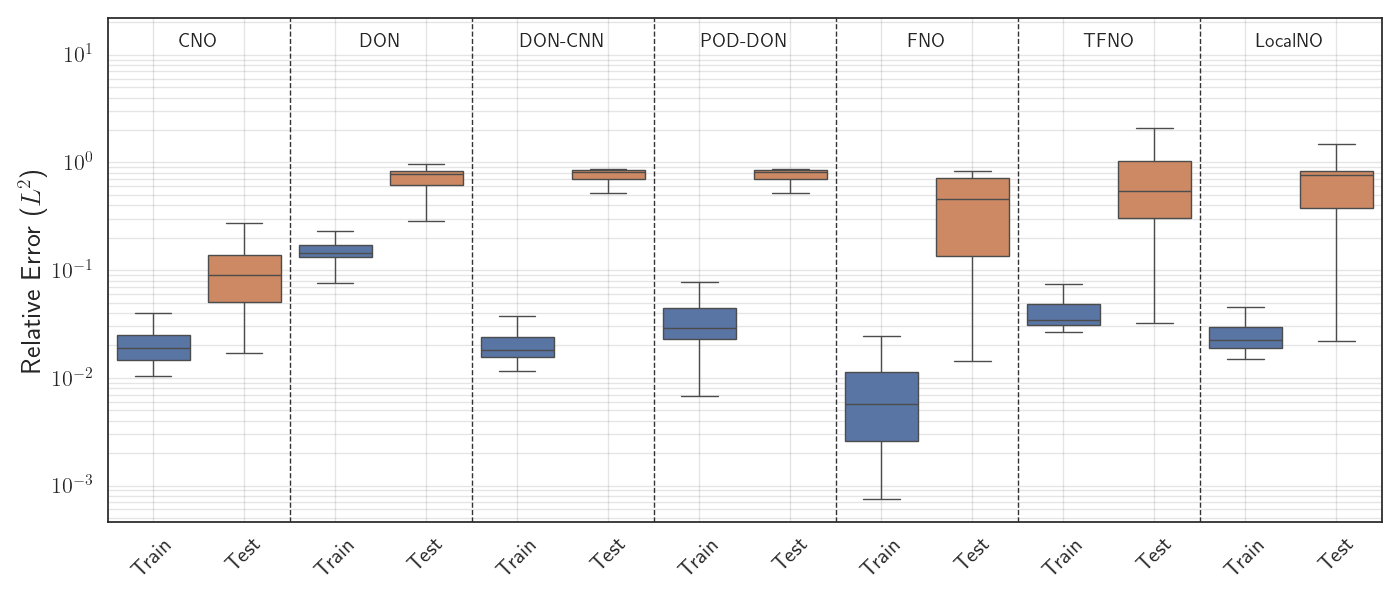
As illustrated in Figure 21, FNO achieve the highest accuracy in the training set. The other architectures exhibit comparable performance, with the exception of DON, which yield a higher error. However, a different trend emerges in the test set, where the models must account for the translated dynamics. Here, only CNO demonstrate the ability to generalize effectively. In contrast, DON and its variants (DON-CNN and POD-DON) faces challenges in replicating the model’s translation invariance property (see Figs. 10, 12, and 14). While FNOs and its variants (TFNOs and LocalNOs) can produce accurate results for certain test examples, but there are many examples with high $\displaystyle L^{2}$ relative errors (see Figs. 15(b), 17(b), and 19(b)). This comparison suggests a trade-off: while FNO is the optimal choice for the training set in terms of accuracy, while CNO provides a more reliable and robust solution for out-of-distribution tasks involving translations. However, accuracy alone is not a comprehensive evaluation of deep learning methods. To provide a more comprehensive comparison, we must also account for computational efficiency, specifically training time and the number of trainable parameters. To this end, we evaluate the following two metrics:

$$\begin{split}&\mathcal{C}\coloneqq E\times P\times T\\ &\mathcal{C}_{log}\coloneqq E\times\Big[1+\alpha\log_{10}(\frac{P}{P_{min}})\Big]\times\Big[1+\beta\log_{10}(\frac{T}{T_{min}})\Big]\\ \end{split}$$

Where $\displaystyle E$ denotes the relative $\displaystyle L^{2}$ error, $\displaystyle P$ is the number of trainable parameters (in millions), and $\displaystyle T$ represents the total training time in hours. The terms $\displaystyle P_{\min}$ and $\displaystyle T_{\min}$ correspond to the minimum number of parameters and the shortest training time, respectively, among all architectures reported in Table 1. The weighting coefficients $\displaystyle\alpha$ and $\displaystyle\beta$ are both fixed at $\displaystyle 0.5$. Figure 22 shows the cost function $\displaystyle\mathcal{C}$ values for training and test errors of each architecture.

Figure 22: Histogram of the $\displaystyle\mathcal{C}$ cost values for each architecture. The cost related to the training error is shown in solid color, while the test is indicated by the hatched pattern.

As illustrated in Figure 22, the FNO has the highest overall cost, primarily due to its large number of trainable parameters (151 M). On the other hand, DON and their variants have the lowest computational cost because of their limited number of parameters and fast training. However, it’s important to note that despite their efficiency, they have difficulty in reproducing the system’s translated dynamics. The CNO has high costs in both training and test, largely due to its intensive computational requirements during training (10 h). Due to the significant differences in scale among these models, we adopted the log-weighted metric $\displaystyle\mathcal{C}_{\text{log}}$. This metric mitigates the significant scale disparities among these models. This ensures a more balanced comparison between compact architectures and over-parameterized models. Figure 23 shows the cost function $\displaystyle\mathcal{C}_{log}$ values for training and test errors of each architecture

Figure 23: Histogram of the $\displaystyle C_{log}$ Cost for each architecture. The cost related to the training error is shown in solid color, while the test is indicated by the hatched pattern.

Figure 23 illustrates the log-weighted cost ($\displaystyle\mathcal{C}_{\text{log}}$), which provides a more fair comparison of the evaluated architectures. The FNO achieves a competitive score because its low training time and training error effectively mitigate the cost associated with its large number of trainable parameters. However, in the test dataset, the FNO and its variants (TFNO and LocalNO) have the highest costs because they cannot maintain reliable performance for the translated dynamics. Similarly, Deep Operator Networks (DONs, DONs-CNN, and POD-DONs) demonstrate consistently high costs for the test dataset, reflecting the difficulty of the generalization for the out-of-distribution scenario. However this models exhibit a lower cost for the training set due to their fast training and limited number of trainable parameters. However, DON-CNN incurs a slightly higher cost than its counterparts due to the added complexity introduced by its encoders. In contrast, the CNO exhibits consistent performance in both training and testing. This stability highlights its unique ability to reliably capture translated dynamics, being the only architecture to do so effectively. Its total cost remains comparable to that of other architectures, mainly due to the high computational cost of training. A final key metric evaluated is the inference latency for a single test instance, compared against the time required to generate a high-fidelity reference solution. This benchmark solution was produced using the Firedrake library [10] on a laptop equipped with an Intel(R) Core(TM) i7-14700HX CPU.

(a) Mean relative $\displaystyle L^{2}$ error vs. inference time.

(b) Median relative $\displaystyle L^{2}$ error vs. inference time.

Figure 24: Comparison of error and inference time for the different architectures. The plots show the inference time relative to the high-fidelity solution time, alongside the accuracy achieved on the training and test sets.

From Figure 24, we can observe a clear trade-off exists between training and test precision and inference efficiency. While the FNO achieves the lowest training error, it is the most computationally expensive architecture during inference. This limitation is also observed in the TFNO variant. DON and their variants, however, emerge as the most efficient models for real-time evaluation. The CNO and LocalNO offer a balanced middle ground. However, we must note that the LocalNO achieves competitive inference speeds due to its limited number of trainable parameters.

5 Conclusion

In this study, we evaluated several Neural Operator architectures, including CNOs, DONs, DONs-CNNs, POD-DONs, FNOs, TFNOs, and LocalNOs, to determine their ability to learn the stiff dynamics and the translation invariance property of the FitzHugh-Nagumo model. We benchmarked these architectures based on their predictive accuracy in training and test datasets, computational efficiency for the training, and inference speed. Our findings reveal that CNOs are the only models capable of accurately reproducing translated dynamics in the test set, achieving a median $\displaystyle L^{2}$ relative error of 0.09. However, this robustness comes at the cost of a higher computational effort for the training, requiring approximately 10 hours for a model with 8.2M trainable parameters. In contrast, despite having a significantly larger number of trainable parameters (151.1M), FNOs required a lower training time (4 hours) than CNOs. However, FNOs and their variants have given less accurate predictions for the translated test cases, with many examples yielding high errors. Furthermore, FNOs and TFNOs suffer from substantial inference costs. The LocalNO variant achieved faster inference, though this was primarily due to its significantly lower number of trainable parameters. Regarding DONs and their variants (DONs-CNN and POD-DONs), we observed that they didn’t generalize well in the translated dynamics of the test set. Nevertheless, DONs architectures demonstrated superior computational efficiency, providing the fastest training and inference speeds among all the models tested. Furthermore, their architecture offers a distinct advantage in terms of flexibility, because they can naturally accommodate non-square geometries without requiring structural modifications. In terms of the training set accuracy, FNOs had the best performance, achieving a relative $\displaystyle L^{2}$ training error of 0.0081. The accuracy of the other architectures was lower though similar to each other. However, our analysis revealed a critical challenge common to all evaluated NOs: determining whether the applied current is sufficient to trigger an action potential, a phenomenon known as the threshold effect. This threshold is difficult to identify because there is no single, precise value for the current. Rather, it depends on the stimulated area and the stimulus duration. For example, incorrectly predicting an action potential when the stimulus is insufficient creates a significant outlier and degrades the NOs ability to accurately capture the correct system dynamics. Future research will focus on improving the ability of NOs to correctly identify whether a stimulus is strong enough to initiate an action potential. In summary, this work provides a rigorous benchmark for NOs, highlighting the trade-offs between computational efficiency and the capacity to learn the stiff dynamics of the FHN model and its translation invariance property.

Author Contributions

LP: Conceptualization, Methodology, Software, Validation, Formal analysis, Investigation, Data Curation, Writing - Original Draft, Writing - Review & Editing, Visualization.

Declarations

Competing Interests The author declare no competing interests.

Data Availability

The code and dataset will be made available on GitHub and Zenodo following the publication of the paper.

Appendix A Model description and dataset generation

This section details the mathematical model under consideration, the dataset generation process, and the range of values employed for the applied current $\displaystyle I_{app}$.

A.1 FitzHugh-Nagumo Model

In this study, we considered the one-dimensional FitzHugh-Nagumo model [6, 7]. Which is a widely used benchmark for capturing the essential dynamics of excitable cells [4]. The system is governed by the following parabolic reaction-diffusion equations:

$$\begin{cases}\chi C_{m}\dfrac{\partial V}{\partial t}-\text{div}(D\nabla V)-\chi bV(V-c)(\delta-V)+\beta w=I_{app},&(x,t)\in[0,1]\times[0,40ms],\\ \dfrac{\partial w}{\partial t}=\eta V-\gamma w,&(x,t)\in[0,1]\times[0,40ms],\end{cases}$$ (9)

where $\displaystyle V$ represents the transmembrane potential and $\displaystyle w$ is the recovery variable. The parameters used in (9) are summarized in Table 2.

Parameter	$\displaystyle\chi$	$\displaystyle C_{m}$	$\displaystyle D$	$\displaystyle b$	$\displaystyle c$	$\displaystyle\delta$	$\displaystyle\beta$	$\displaystyle\eta$	$\displaystyle\gamma$
Value	1	1	0.001	5	0.1	1	1	0.1	0.25

Table 2: Parameters assigned to the FHN model in (9).

A.2 Dataset generation

The dataset was generated using Firedrake [10], a finite element library. For the spatial discretization, were employed second-degree Lagrange polynomials over a mesh consisting of 200 intervals. Temporal integration was performed using the forward Euler method with a constant time step of $\displaystyle\Delta t=0.05$. We solved the resulting nonlinear systems using the Newton method, and we handled the underlying linear systems using the generalized minimal residual method. To ensure efficient convergence, we utilized a generalized additive Schwarz method as a preconditioner. The applied current, as defined in (3), the stimulated region is defined as:

$$\Omega_{T,stim}=[x_{\min},x_{\min}+0.04]\times[T_{\min},T_{\min}+1].$$

The parameter ranges and values used for the training, validation, and test datasets are summarized in Table 3.

Name	Range of values of $\displaystyle i$		Time of the stimulus	Position of the stimulus	Number of examples
	min	max	$\displaystyle T_{min}$	$\displaystyle x_{min}$
Train	0.1	3	5	0-0.96	2000
Validation / Test	0.1	3	0-37	0-0.96	500

Table 3: FHN model: Range of values of the training, validation and test set.

Appendix B Automatic hyperparameter tuning

In this section, we provide details on the automatic hyperparameter tuning used for each of the architectures considered in this work. We performed 100 distributed and parallel trials for each architecture, employing an automatic hyperparameter optimization algorithm implemented in the HyperOptSearch library. In particular, we employed the Tree-structured Parzen Estimator algorithm [3], and the ASHA scheduler [19] to automatically stop trials that were not satisfactory. Each model was trained using the data-driven relative $\displaystyle L^{2}$ norm as the loss function.

$$\begin{split}\text{Loss}\left(u,\,\mathcal{G}_{\theta}(I_{app})\right)&=\frac{1}{2}\sum_{j=1}^{2}\frac{\|u_{j}-\mathcal{G}_{\theta}(I_{app})_{j}\|_{L^{2}(\Omega_{T})}}{\|u_{j}\|_{L^{2}(\Omega_{T})}}\\ &\approx\frac{1}{2}\sum_{j=1}^{2}\frac{\left(\sum_{k=1}^{n_{points}}|u_{j}(x_{k},t_{k})-\mathcal{G}_{\theta}(I_{app})_{j}(x_{k},t_{k})|^{2}\right)^{1/2}}{\left(\sum_{k=1}^{n_{points}}|u_{j}(x_{k},t_{k})|^{2}\right)^{1/2}},\end{split}$$

where $\displaystyle u$ is the solution of the system (1) and $\displaystyle\mathcal{G}_{\theta}$ is the operator defined in (4). This leads to the following optimization problem:

$$\underset{\theta\in\Theta}{\arg\min}\ \ \frac{1}{n_{train}}\sum_{i=1}^{n_{train}}\text{Loss}\left(u^{i},\,\mathcal{G}_{\theta}(I_{app}^{i})\right),$$

where $\displaystyle\{(I_{app}^{i},u^{i})\}_{i=1}^{n_{train}}$ is the dataset consisted of input-output pairs.

B.1 Convolutional Neural Operators hyperparameters

Table 4 summarizes the hyperparameters for the CNOs [27], detailing the configuration of the search space and the optimal values identified by the automatic hyperparameter tuning.

Hyperparameter	Description	Search Space	Found
Architecture
$\displaystyle N_{\text{layers}}$	Number of layers of the U-Net	$\displaystyle 1\leq N_{\text{layers}}\leq 5$	4
C	Dimension of channel multiplier	C$\displaystyle\in\{8,16,24,32,40,48\}$	32
$\displaystyle N_{\text{res,neck}}$	Number residual block of the last layer	$\displaystyle 1\leq N_{\text{res,neck}}\leq 6$	2
$\displaystyle N_{\text{res}}$	Number residual block	$\displaystyle 1\leq N_{\text{res}}\leq 8$	7
$\displaystyle k$	Kernel size	$\displaystyle k\in\{3,5,7\}$	3
Optimizer
$\displaystyle\eta$	Initial learning rate	1e-4 $\displaystyle\leq\eta\leq$1e-2	1.9e-4
$\displaystyle\omega$	Weight decay regularization factor	1e-6 $\displaystyle\leq\omega\leq$1e-3	3.2e-3
$\displaystyle\gamma$	Rate scheduler factor	$\displaystyle 0.75\leq\gamma\leq 0.99$	0.91

Table 4: CNOs hyperparameters and the search space used for hyperparameter tuning.

B.2 Deep Operator Network hyperparameters

The DONs implementation is taken from the DeepXDE library [25]. Table 5 summarizes the hyperparameters for the DONs [23], detailing the configuration of the search space and the optimal values identified by the automatic hyperparameter tuning.

Hyperparameter	Description	Search Space	Found
$\displaystyle p$	Number of basis functions	$\displaystyle 200\leq p\leq 800$	762
Branch Network
$\displaystyle N_{branch}$	Number of hidden layers	$\displaystyle 1\leq N_{branch}\leq 6$	6
$\displaystyle W_{branch}$	Network width (neurons)	$\displaystyle 64\leq W_{branch}\leq 200$	124
$\displaystyle\sigma_{branch}$	Activation function	$\displaystyle\sigma_{branch}\in$ {relu, gelu, silu}	relu
Trunk Network
$\displaystyle N_{trunk}$	Number of hidden layers	$\displaystyle 1\leq N_{trunk}\leq 6$	4
$\displaystyle W_{trunk}$	Network width (neurons)	$\displaystyle 64\leq W_{trunk}\leq 200$	148
$\displaystyle\sigma_{trunk}$	Activation function	$\displaystyle\sigma_{trunk}\in$ {relu, gelu, silu}	relu
Optimizer
$\displaystyle\eta$	Initial learning rate	$\displaystyle 10^{-4}\leq\eta\leq 10^{-2}$	1.8e-3
$\displaystyle\omega$	Weight decay factor	$\displaystyle 10^{-6}\leq\omega\leq 10^{-3}$	4.5e-4
$\displaystyle\gamma$	Rate scheduler factor	$\displaystyle 0.75\leq\gamma\leq 0.99$	97

Table 5: DONs hyperparameters and the search space used for hyperparameter tuning.

B.3 Deep Operator Network with CNN encoders hyperparameters

Table 6 summarizes the hyperparameters for the DONs-CNN, detailing the configuration of the search space and the optimal values identified by the automatic hyperparameter tuning.

Hyperparameter	Description	Search Space	Found
$\displaystyle p$	Number of basis functions	$\displaystyle 200\leq p\leq 500$	332
Branch Network
$\displaystyle N_{conv}$	Number of convolutional layers	$\displaystyle 3\leq N_{conv}\leq 7$	3
$\displaystyle C_{start}$	Starting number of channels (first layer)	$\displaystyle C_{start}\in\{10,20,30,40\}$	40
$\displaystyle C_{step}$	Channel increment per layer	$\displaystyle C_{step}\in\{10,20,30\}$	30
$\displaystyle C_{ch}$	Channel configuration	-	[40, 70, 100]
$\displaystyle N_{FNN,branch}$	Number of layers for the FNN	$\displaystyle 2\leq N_{FNN,branch}\leq 7$	3
$\displaystyle N_{neuron,branch}$	Number of neurons per dense layer	$\displaystyle N_{neuron,branch}\in\{16,32,64,128,256\}$	16
$\displaystyle\sigma_{branch}$	Activation function	$\displaystyle\sigma_{branch}\in\{\text{tanh, relu, leaky\_relu, sigmoid, silu, gelu}\}$	relu
Normalization	Type of layer normalization	Normalization $\displaystyle\in\{\text{none, batch, layer}\}$	none
Trunk Network
$\displaystyle N_{FNN,trunk}$	Number of layers for the FNN	$\displaystyle 2\leq N_{FNN,trunk}\leq 7$	4
$\displaystyle N_{neuron,trunk}$	Number of neurons per dense layer	$\displaystyle N_{neuron,trunk}\in\{16,32,64,128,256\}$	16
$\displaystyle\sigma_{trunk}$	Activation function	$\displaystyle\sigma_{trunk}\in\{\text{tanh, relu, leaky\_relu, sigmoid}\}$	leaky_relu
Architecture	Use of residual connections	Classic or Residual	Classical
Layer Norm	Apply layer normalization	True or False	False
Optimizer
$\displaystyle\eta$	Initial learning rate	1e-4$\displaystyle\leq\eta\leq$ 1e-2	6.6e-3
$\displaystyle\omega$	Weight decay regularization factor	1e-6$\displaystyle\leq\omega\leq$ 1e-3	4.6e-4
$\displaystyle\gamma$	Rate scheduler factor	$\displaystyle 0.75\leq\gamma\leq 0.99$	0.84

Table 6: DONs-CNN hyperparameters and the search space used for hyperparameter tuning

B.4 Proper Orthogonal Decomposition DeepONets hyperparameters

The POD-DONs implementation is taken from the DeepXDE library [25]. Table 7 summarizes the hyperparameters for the POD-DONs [24], detailing the configuration of the search space and the optimal values identified by the automatic hyperparameter tuning.

Hyperparameter	Description	Search Space	Found
$\displaystyle p$	Number of basis functions ($\displaystyle n\_basis$)	$\displaystyle 200\leq p\leq 800$	500
Branch Network
$\displaystyle N_{branch}$	Number of hidden layers	$\displaystyle 1\leq N_{branch}\leq 6$	6
$\displaystyle W_{branch}$	Network width	$\displaystyle 64\leq W_{branch}\leq 200$	92
$\displaystyle\sigma_{branch}$	Activation function	$\displaystyle\sigma_{branch}\in$ {relu, gelu, silu}	gelu
Optimizer
$\displaystyle\eta$	Initial learning rate	1e-4$\displaystyle\leq\eta\leq$1e-2	$\displaystyle 6.7\times 10^{-4}$
$\displaystyle\omega$	Weight decay factor	1e-6$\displaystyle\leq\omega\leq$1e-3	$\displaystyle 4.25\times 10^{-4}$
$\displaystyle\gamma$	Rate scheduler factor	$\displaystyle 0.75\leq\gamma\leq 0.99$	0.92

Table 7: POD-DONs hyperparameters and the search space used for hyperparameter tuning.

B.5 Fourier Neural Operators hyperparameters

Table 8 summarizes the hyperparameters for the FNOs [20], detailing the configuration of the search space and the optimal values identified by the automatic hyperparameter tuning.

Hyperparameter	Description	Search Space	Found
Architecture
$\displaystyle 0pt$	Hidden dimension	$\displaystyle 0pt\in\{4,8,16,32,64,96,128,160,192,220\}$	128
$\displaystyle L$	Number of hidden layers	1 $\displaystyle\leq L\leq$6	4
$\displaystyle k_{max}$	Number of Fourier modes	$\displaystyle k_{max}\in\{2,4,8,12,16,20,24,28,32\}$	24
$\displaystyle\sigma$	Activation function	$\displaystyle\sigma\in${tanh, relu, gelu, leaky_relu}	relu
$\displaystyle n_{pad}$	Number of padding points per direction	1$\displaystyle\leq n_{pad}\leq$16	1
Architecture	Fourier architecture (7), (8) or residual	Classic, MLP or Residual	Classic
Optimizer
$\displaystyle\eta$	Initial learning rate	1e-4 $\displaystyle\leq\eta\leq$ 1e-2	1.8e-3
$\displaystyle\omega$	Weight decay regularization factor	1e-6 $\displaystyle\leq\omega\leq$ 1e-3	4e-6
$\displaystyle\gamma$	Rate scheduler factor	$\displaystyle 0.75\leq\gamma\leq 0.99$	0.85

Table 8: FNOs hyperparameters and the search space used for hyperparameter tuning.

B.6 Tucker Tensorized FNOs hyperparameters

The TFNOs implementation is taken from the Neural Operator library [15]. Table 9 summarizes the hyperparameters for the TFNOs [31], detailing the configuration of the search space and the optimal values identified by the automatic hyperparameter tuning.

Hyperparameter	Description	Search Space	Found
Architecture
$\displaystyle 0pt$	Hidden dimension	$\displaystyle 0pt\in\{4,8,16,\dots,192\}$	192
$\displaystyle L$	Number of hidden layers	$\displaystyle 1\leq L\leq 5$	1
$\displaystyle k_{max}$	Number of Fourier modes	$\displaystyle k_{max}\in\{2,4,8,\dots,32\}$	8
$\displaystyle\sigma$	Activation function	$\displaystyle\sigma\in$ {gelu, relu, leaky_relu}	leaky_relu
Domain Padding	Domain padding fraction	$\displaystyle\{0,0.1,0.2\}$	0.2
MLP skip	Skip connection in MLP	{Linear, identity, soft-gating, None}	identity
FNO skip	Skip connection in FNO	{Linear, identity, soft-gating, None}	soft-gating
MLP	Usage of Channel MLP	True or False	False
Rank	Tensor rank ratio	$\displaystyle\{0.05,0.1,0.2,0.5\}$	0.2
Optimizer
$\displaystyle\eta$	Initial learning rate	1e-4$\displaystyle\leq\eta\leq$1e-2	5.5e-3
$\displaystyle\omega$	Weight decay factor	1e-6$\displaystyle\leq\omega\leq$ 1e-3	5.5e-4
$\displaystyle\gamma$	Rate scheduler factor	$\displaystyle 0.75\leq\gamma\leq 0.99$	0.8

Table 9: TFNOs hyperparameters and the search space used for hyperparameter tuning.

B.7 Local Neural Operators hyperparameters

The LocalNOs implementation is taken from the Neural Operator library [15]. Table 10 summarizes the hyperparameters for the LocalNOs [22], detailing the configuration of the search space and the optimal values identified by the automatic hyperparameter tuning.

Hyperparameter	Description	Search Space	Found
Architecture
$\displaystyle 0pt$	Hidden dimension	$\displaystyle 0pt\in\{4,8,16,32,64,96,128,160,192\}$	8
$\displaystyle L$	Number of hidden layers	1 $\displaystyle\leq L\leq$6	2
$\displaystyle k_{max}$	Number of Fourier modes	$\displaystyle k_{max}\in\{2,4,8,12,16,20,24,28,32\}$	24
$\displaystyle\sigma$	Activation function	$\displaystyle\sigma\in${relu, gelu, leaky_relu}	relu
Padding	Type of padding	reflect or zeros	zeros
Factorization	Type of Factorization	None, Tucker, CP, TT	TT
MLP skip	Skip connection in MLP	Linear, identity and soft-gating	linear
local skip	Skip connection in LocalNO	Linear, identity and soft-gating	identity
Differential kernel size	Finite difference kernel size	{3,5,7}	7
MLP	Usage of MLP	True or False	True
Rank	Tensor rank for factorization	{0.05,0.1,0.2,0.5,1}	0.1
Disco Layer	Usage of Disco (integral) layer	True or False	False
Optimizer
$\displaystyle\eta$	Initial learning rate	1e-4 $\displaystyle\leq\eta\leq$ 1e-2	1.4e-3
$\displaystyle\omega$	Weight decay regularization factor	1e-6 $\displaystyle\leq\omega\leq$ 1e-3	2.8e-4
$\displaystyle\gamma$	Rate scheduler factor	$\displaystyle 0.75\leq\gamma\leq 0.99$	0.97

Table 10: LocalNOs hyperparameters and the search space used for hyperparameter tuning.

References

- [1] (2024) Neural operators for accelerating scientific simulations and design. Nature Reviews Physics 6 (5), pp. 320–328. Cited by: §2.1.
- [2] (2023) Are neural operators really neural operators? frame theory meets operator learning. SAM Research Report 2023. Cited by: §2.1.
- [3] (2011) Algorithms for hyper-parameter optimization. Advances in neural information processing systems 24. Cited by: Appendix B.
- [4] (2024) Six decades of the fitzhugh–nagumo model: a guide through its spatio-temporal dynamics and influence across disciplines. Physics Reports 1096, pp. 1–39. Cited by: §A.1, §1.
- [5] (2024) Learning the hodgkin–huxley model with operator learning techniques. Computer Methods in Applied Mechanics and Engineering 432, pp. 117381. Cited by: §1, §2.1.
- [6] (2014) Mathematical Cardiac Electrophysiology. Vol. 13, Springer, Cham. Cited by: §A.1, §1.
- [7] (1961) Impulses and physiological states in theoretical models of nerve membrane. Biophysical Journal 1 (6), pp. 445–466. Cited by: §A.1, §1.
- [8] (2025) NOBLE–neural operator with biologically-informed latent embeddings to capture experimental variability in biological neuron models. arXiv preprint arXiv:2506.04536. Cited by: §1.
- [9] (2025) HyperNOs: Automated and Parallel Library for Neural Operators Research. arXiv preprint arXiv:2503.18087. Cited by: §2.1.1, §3.
- [10] (2023-05) Firedrake user manual. First edition edition, Imperial College London and University of Oxford and Baylor University and University of Washington. External Links: Document Cited by: §A.2, Figure 1, Figure 1, Figure 2, Figure 2, Figure 3, Figure 3, §4.
- [11] (1952) A quantitative description of membrane current and its application to conduction and excitation in nerve. The Journal of Physiology 117 (4), pp. 500. Cited by: §1.
- [12] (2025) Physics-informed neural network estimation of active material properties in time-dependent cardiac biomechanical models. arXiv preprint arXiv:2505.03382. Cited by: §1.
- [13] (2007) Dynamical systems in neuroscience. MIT press. Cited by: §1.
- [14] (2009) Mathematical physiology: ii: systems physiology. Springer. Cited by: §1.
- [15] (2025) A library for learning neural operators. arXiv preprint arXiv:2412.10354. Cited by: §B.6, §B.7.
- [16] (2023) Neural operator: learning maps between function spaces with applications to pdes. Journal of Machine Learning Research 24 (89), pp. 1–97. Cited by: §1, §2.1.2.
- [17] (2023) Neural operator: Learning maps between function spaces with applications to pdes. Journal of Machine Learning Research 24 (89), pp. 1–97. Cited by: §2.1.1, §2.1.3, §2.1.
- [18] (2023) Nonlocality and nonlinearity implies universality in operator learning. arXiv preprint arXiv:2304.13221. Cited by: §2.1.
- [19] (2020) A system for massively parallel hyperparameter tuning. Proceedings of machine learning and systems 2, pp. 230–246. Cited by: Appendix B.
- [20] (2020) Fourier neural operator for parametric partial differential equations. arXiv preprint arXiv:2010.08895. Cited by: §B.5, §1, §2.1.3, §3.5.
- [21] (2018) Tune: A Research Platform for Distributed Model Selection and Training. arXiv preprint arXiv:1807.05118. Cited by: §3.
- [22] (2024) Neural operators with localized integral and differential kernels. arXiv preprint arXiv:2402.16845. Cited by: §B.7, §1, 1st item, §3.7.
- [23] (2021) Learning nonlinear operators via DeepONet based on the universal approximation theorem of operators. Nature Machine Intelligence 3 (3), pp. 218–229. Cited by: §B.2, §1, §2.1.2, §3.2.
- [24] (2022) A comprehensive and fair comparison of two neural operators (with practical extensions) based on fair data. Computer Methods in Applied Mechanics and Engineering 393, pp. 114778. Cited by: §B.4, §1, 2nd item, §3.4.
- [25] (2021) DeepXDE: a deep learning library for solving differential equations. SIAM Review 63 (1), pp. 208–228. External Links: Document Cited by: §B.2, §B.4.
- [26] (2025) Learning high-dimensional ionic model dynamics using fourier neural operators. Machine Learning for Computational Science and Engineering 1 (2), pp. 46. Cited by: §1, §2.1.
- [27] (2023) Convolutional neural operators. ICLR 2023 Workshop on Physics for Machine Learning. Cited by: §B.1, §1, §2.1.1, §2.1.1, §3.1.
- [28] (2015) U-net: convolutional networks for biomedical image segmentation. In International Conference on Medical image computing and computer-assisted intervention, pp. 234–241. Cited by: §2.1.1.
- [29] (2024) Whole-heart electromechanical simulations using latent neural ordinary differential equations. NPJ Digital Medicine 7 (1), pp. 90. Cited by: §1.
- [30] (2024) Splitting physics-informed neural networks for inferring the dynamics of integer-and fractional-order neuron models. Communications in Computational Physics 35 (1), pp. 1–37. Cited by: §1.
- [31] (2026) Tucker-FNO: tensor tucker-fourier neural operator and its universal approximation theory. In The Fourteenth International Conference on Learning Representations, External Links: Link Cited by: §B.6, §1, 2nd item, §3.6.
- [32] (2026) Learning cardiac activation and repolarization times with operator learning. PLOS Computational Biology 22 (1), pp. e1013920. Cited by: §1.