Perturbation Analysis for Preconditioned
Normal Equations in Mixed Precision

Abstract

For real matrices of full column-rank, we analyze the conditioning of several types of normal equations that are preconditioned by a randomized preconditioner computed in lower precision. These include symmetrically preconditioned normal equations, half-preconditioned normal equations, seminormal equations and not-normal equations. Our perturbation bounds are realistic and informative, and suggest that the conditioning depends only mildly on the quality of the preconditioner; however, it does depend on the size of the least squares residual – even if the normal equations do not originate from a least squares problem. We illustrate that a randomized preconditioner can deliver a solution accuracy comparable to that of Matlab’s mldivide command, is efficient in practice, and well-suited to GPU implementations. For the computation of the preconditioner, we propose an automatic selection of the precision, based on a fast condition number estimation in lower precision.

65F45, 65F20, 15A12

1 Introduction

Given a matrix $\boldsymbol{A}\in{\mathbb{R}}^{m\times n}$ with $\operatorname{\mathrm{rank}}(\boldsymbol{A})=n$, and $\boldsymbol{b}\in\mathbb{R}^{m}$, we consider the conditioning of the normal equations

(1) $$\boldsymbol{A}^{T}\boldsymbol{A}\boldsymbol{x}=\boldsymbol{A}^{T}\boldsymbol{b}.$$

Although normal equations represent a simple and effective solution of least squares problems

(2) $$\|\boldsymbol{A}\boldsymbol{x}-\boldsymbol{b}\|_{2}=\min_{\boldsymbol{x}}{\|\boldsymbol{A}\boldsymbol{x}-\boldsymbol{b}\|_{2}},$$

they can be illconditioned and are not recommended in many applications [9, Section 5.3.7]. For instance, once the condition number of $\boldsymbol{A}$ with respect to left inversion exceeds $10^{7}$, then $\boldsymbol{A}^{T}\boldsymbol{A}$ is numerically singular in IEEE double precision. Hence, for the normal equations to be well conditioned and safe to use, the condition number of $\boldsymbol{A}$ must be small, ideally close to 1.

We analyze two preconditioning approaches from [12] for improving the conditioning of the normal equations, but now with the preconditioner computed in lower precision.

Preconditioned Normal Equations (PNE).

Precondition the matrix $\boldsymbol{A}$ with a randomized preconditioner $\boldsymbol{R}_{s}$ so that the preconditioned matrix $\boldsymbol{A}_{p}\equiv\boldsymbol{A}\boldsymbol{R}_{s}^{-1}$ is well conditioned with high probability. Then solve the preconditioned normal equations and recover the original solution,

(3) $$\begin{split}\boldsymbol{A}_{p}^{T}\boldsymbol{A}_{p}\boldsymbol{y}&=\boldsymbol{A}_{p}^{T}\boldsymbol{b}\\ \boldsymbol{R}_{s}\boldsymbol{x}&=\boldsymbol{y}.\end{split}$$

Half Preconditioned Normal Equations (HPNE).

Dispense with the triangular system solution by preconditioning only the left instances of $\boldsymbol{A}$,

(4) $$\boldsymbol{A}_{p}^{T}\boldsymbol{A}\boldsymbol{x}=\boldsymbol{A}_{p}^{T}\boldsymbol{b}.$$

Since $\boldsymbol{A}_{p}^{T}\boldsymbol{A}$ is non-symmetric, the linear system has to be solved by an LU factorization with partial pivoting, a QR factorization, or an iterative solver. The HPNE (4) represent a special case of the not-normal equations [21],

$$\boldsymbol{B}^{T}\boldsymbol{A}\boldsymbol{x}=\boldsymbol{B}^{T}\boldsymbol{b},$$

where $\boldsymbol{B}\in{\mathbb{R}}^{m\times n}$ is a full column rank matrix with the same column space as $\boldsymbol{A}$.

The perturbation analysis in [12] suggests that PNE and HPNE, with an effective preconditioner so that $\kappa(\boldsymbol{A}_{p})\lesssim 10$, are as well conditioned as $\boldsymbol{A}$, and their solution can be almost as accurate as that from the Matlab backslash ($\verb|mldivide|$) command. However, the bounds from [12] are not informative if the preconditioner is computed in a lower precision. In contrast, our new bounds for PNE and HPNE in Sections 3 and 4 are realistic, as illustrated in Figure 1.

Figure 1: Relative errors $\|\boldsymbol{\hat{\boldsymbol{x}}}-\boldsymbol{x}_{*}\|/\|\boldsymbol{\hat{\boldsymbol{x}}}\|$ in the computed solutions $\boldsymbol{\hat{\boldsymbol{x}}}$ and perturbation bounds versus logarithm of relative least squares residuals $\|\boldsymbol{b}-\boldsymbol{A}\boldsymbol{x}_{*}\|/(\|\boldsymbol{A}\|\|\boldsymbol{x}_{*}\|)$ for $\boldsymbol{A}\in\mathbb{R}^{1,000\times 100}$ with condition number $\kappa(\boldsymbol{A})=10^{8}$. Shown are the Matlab backslash solutions (red plusses); the HPNE solutions with a single precision preconditioner (blue squares); the generalized version (34) of the perturbation bound [12, Theorem 3.1] (green circles); and our new bound (35) (black x’s).

1.1 Contributions and Overview

We present perturbation bounds for PNE and HPNE when the preconditioner is computed in lower precision, and illustrate the potential for faster speed.

1. Our perturbation bounds are realistic and informative for both PNE (Theorem 3.3 in Section 3.2) and HPNE (Theorem 4.3 in Section 4.2), and imply that their conditioning depends only very weakly on the preconditioner $\boldsymbol{R}_{s}$.

2. The mixed precision solution of PNE and HPNE by direct methods on NVIDIA H100 GPUs shows potential for speedups over established direct methods (Section 7.4).

3. Our perturbation bound for the seminormal equations (Section 5.1) implies that they are no better conditioned than the normal equations.

4. Like for PNE and HPNE, the perturbation bound for the not-normal equations (Section 5.2) depends on the least squares residual and implies that they are well conditioned when they are close to the HPNE.

5. We propose an automatic selection of the precision level, based on a fast condition number estimation in the lower precision (Algorithm 1 in Section 6).

Overview.

After defining notation (Section 1.2), we review existing work (Section 2), followed by perturbation bounds for the PNE (Section 3) and the HPNE (Section 4), as well as for the seminormal and not-normal equations (Section 5). We present the randomized preconditioner in lower precision (Section 6) and end with numerical experiments (Section 7).

1.2 Notation

For a matrix $\boldsymbol{A}\in{\mathbb{R}}^{m\times n}$ with $\operatorname{\mathrm{rank}}(\boldsymbol{A})=n$, the Moore-Penrose inverse is $\boldsymbol{A}^{\dagger}\equiv(\boldsymbol{A}^{T}\boldsymbol{A})^{-1}\boldsymbol{A}^{T}$, and the two-norm condition number with respect to left inversion is $\kappa(\boldsymbol{A})\equiv\|\boldsymbol{A}\|\|\boldsymbol{A}^{\dagger}\|$, where $\|\cdot\|$ denotes the Euclidean two-norm.

To put subsequent bounds in context, we review perturbation bounds for least squares problems (2), and the normal equations (1).

Lemma 1.1 (Fact 5.14 in [11]).

Let $\boldsymbol{A},\boldsymbol{A}+\boldsymbol{E}\in{\mathbb{R}}^{m\times n}$ with $\operatorname{\mathrm{rank}}(\boldsymbol{A})=\operatorname{\mathrm{rank}}(\boldsymbol{A}+\boldsymbol{E})=n$ and $\epsilon_{A}\equiv\|\boldsymbol{E}\|/\|\boldsymbol{A}\|$. Let $\boldsymbol{x}_{*}$ be the solution to $\min_{\boldsymbol{x}}{\|\boldsymbol{A}\boldsymbol{x}-\boldsymbol{b}\|}$ and $\boldsymbol{\hat{\boldsymbol{x}}}\neq\boldsymbol{0}$ the solution to $\min_{\boldsymbol{x}}{\|(\boldsymbol{A}+\boldsymbol{E})\boldsymbol{x}-\boldsymbol{b}\|}$. Then

$$\frac{\|\boldsymbol{\hat{\boldsymbol{x}}}-\boldsymbol{x}_{*}\|}{\|\boldsymbol{\hat{\boldsymbol{x}}}\|}\leq\kappa(\boldsymbol{A})\,\epsilon_{A}\,\left(1+\kappa(\boldsymbol{A})\frac{\|\boldsymbol{b}-(\boldsymbol{A}+\boldsymbol{E})\boldsymbol{\hat{\boldsymbol{x}}}\|}{\|\boldsymbol{A}\|\|\boldsymbol{\hat{\boldsymbol{x}}}\|}\right).$$

We do not consider perturbations in the right hand side $\boldsymbol{b}$, because perturbations in $\boldsymbol{A}$ tend to be more influential on the sensitivity of the least squares problems.

The following bound for the normal equations makes no assumptions on the perturbation $\boldsymbol{E}$, so that $\boldsymbol{A}+\boldsymbol{E}$ can be rank deficient.

Lemma 1.2 (Lemma A.1 in [12]).

Let $\boldsymbol{A},\boldsymbol{A}+\boldsymbol{E}\in{\mathbb{R}}^{m\times n}$ with $\operatorname{\mathrm{rank}}(\boldsymbol{A})=n$; $\epsilon_{A}\equiv\|\boldsymbol{A}\|/\|\boldsymbol{E}\|$; and

$$\boldsymbol{A}^{T}\boldsymbol{A}\boldsymbol{x}_{*}=\boldsymbol{A}^{T}\boldsymbol{b},\qquad(\boldsymbol{A}+\boldsymbol{E})^{T}(\boldsymbol{A}+\boldsymbol{E})\boldsymbol{\hat{\boldsymbol{x}}}=(\boldsymbol{A}+\boldsymbol{E})^{T}\boldsymbol{b}.$$

If $\boldsymbol{\hat{\boldsymbol{x}}}\neq\boldsymbol{0}$ then

$$\frac{\|\boldsymbol{\hat{\boldsymbol{x}}}-\boldsymbol{x}_{*}\|}{\|\boldsymbol{\hat{\boldsymbol{x}}}\|}\leq\kappa(\boldsymbol{A})^{2}\epsilon_{A}\>\left(\frac{\|\boldsymbol{b}-\boldsymbol{A}\boldsymbol{\hat{\boldsymbol{x}}}\|}{\|\|\boldsymbol{A}\|\|\boldsymbol{\hat{\boldsymbol{x}}}\|}+1+\epsilon_{A}\right).$$

Lemma 1.2 suggests that the accuracy of the normal equations only depends on the least squares residual when it is too large, $\frac{\|\boldsymbol{b}-\boldsymbol{A}\boldsymbol{\hat{\boldsymbol{x}}}\|}{\|\boldsymbol{A}\|\|\boldsymbol{\hat{\boldsymbol{x}}}\|}>1$.

2 Existing Work

The use of normal equations is often discouraged due to the ’matrix squaring problem,’ where $\kappa(\boldsymbol{A}^{T}\boldsymbol{A})=\kappa(\boldsymbol{A})^{2}$, leading to a potentially much worse conditioned linear system. Preconditioning the normal equations is not obvious, as effective preconditioners for $\boldsymbol{A}$ do not necessarily make effective preconditioners for $\boldsymbol{A}^{T}\boldsymbol{A}$ [20].

Nonsymmetric systems $\boldsymbol{A}\boldsymbol{x}=\boldsymbol{b}$ can be solved by applying preconditioned iterative methods such as CGNE to the normal equations [9, Section 11.3.9.], [17]. In [14], CGNE preconditioners are constructed for linear systems that arise from certain PDE discretizations. In [21], the iterative solution of the not-normal equations $\boldsymbol{B}^{T}\boldsymbol{A}\boldsymbol{x}=\boldsymbol{B}^{T}\boldsymbol{b}$ is proposed, where $\boldsymbol{B}\in{\mathbb{R}}^{m\times n}$ has the same column space of $\boldsymbol{A}$ and can be obtained from an LU factorization of $\boldsymbol{A}$.

The iterative solution of preconditioned normal equations with iterative refinement via backward stable algorithms is presented in [7, 22]. The corresponding FOSSILS/SPIR and SIRR algorithms have an operation count of $\mathcal{O}(mn+n^{3})$. An alternative use of iterative refinement for least squares problems is to iteratively refine the seminormal equations $\boldsymbol{R}^{T}\boldsymbol{R}\boldsymbol{x}=\boldsymbol{A}^{T}\boldsymbol{b}$ [4], where it is observed that the seminormal equations, when combined with iterative refinement, are not sensitive to the size of the relative least squares residual.

Although algorithms like FOSSILS and SIRR are numerically stable, the cost of computing the preconditioner remains an issue. Mixed-precision approaches can reduce this cost. For linear systems, Higham and Pranesh [10] propose Cholesky factorizations in lower precision as preconditioners for iterative refinement and extend this to the solution of least squares problems via normal equations. Similarly, Scott and Tůma [19] compute incomplete Cholesky factors in lower precision to precondition LSQR. Li [15] also investigates mixed-precision within the LSQR algorithm for solving discrete linear ill-posed problems via regularized least squares.

Beyond low-precision factorizations, many randomized sketching techniques are inherently parallelizable and can benefit from GPU acceleration. Chen et. al. [6] give a thorough benchmarking of a GPU-based sketch-and-precondition solver based on a sparse sign embedding. Carson and Daužickaitė [5] compute a mixed-precision sketch as the preconditioner for GMRES with iterative refinement.

3 Preconditioned Normal Equations (PNE)

We extend an existing PNE perturbation bound to mixed precision (Section 3.1) and then present an improvement (Section 3.2).

3.1 Extension of an existing PNE perturbation bound to mixed precision

A previous bound [12, Theorem 2.1] shows that the conditioning of the PNE depends on the least squares residual of the original least squares problem. Theorem 3.1 below is a small extension where the preconditioner can be computed in a different precision.

Theorem 3.1.

Let $\boldsymbol{A}\in{\mathbb{R}}^{m\times n}$ have $\operatorname{\mathrm{rank}}(\boldsymbol{A})=n$; $\boldsymbol{R}_{s}\in{\mathbb{R}}^{n\times n}$ be nonsingular; $\boldsymbol{E}_{s}\in{\mathbb{R}}^{n\times n}$, $\boldsymbol{E}_{A}\in{\mathbb{R}}^{m\times n}$;

$$\boldsymbol{A}_{1}\equiv\boldsymbol{A}(\boldsymbol{R}_{s}+\boldsymbol{E}_{s})^{-1},\qquad\boldsymbol{A}_{2}\equiv\boldsymbol{A}_{p}+\boldsymbol{E}_{p},\qquad\epsilon_{s}\equiv\frac{\|\boldsymbol{E}_{s}\|}{\|\boldsymbol{R}_{s}\|},\qquad\epsilon_{p}\equiv\frac{\|\boldsymbol{E}_{p}\|}{\|\boldsymbol{A}_{p}\|};$$

and $\|\boldsymbol{E}_{s}\|\|\boldsymbol{R}_{s}^{-1}\|<1$. The computed solutions corresponding to (3) are

(5) $$\boldsymbol{A}_{1}^{T}\boldsymbol{A}_{2}\boldsymbol{\hat{\boldsymbol{x}}} =\boldsymbol{A}_{1}^{T}\boldsymbol{b}$$

(6) $$\boldsymbol{R}_{s}\boldsymbol{\hat{\boldsymbol{x}}} =\boldsymbol{\hat{y}}.$$

If $\boldsymbol{\hat{\boldsymbol{x}}}\neq\boldsymbol{0}$ and $\boldsymbol{\hat{y}}\neq\boldsymbol{0}$, then

$$\frac{\|\boldsymbol{x}_{*}-\boldsymbol{\hat{\boldsymbol{x}}}\|}{\|\boldsymbol{\hat{\boldsymbol{x}}}\|}\leq\kappa(\boldsymbol{R}_{s})\kappa(\boldsymbol{A}_{p})\,\nu\,\left(\epsilon_{p}+\kappa(\boldsymbol{A}_{p})\,\eta_{s}\left(\frac{\|\boldsymbol{A}_{p}\boldsymbol{\hat{y}}-\boldsymbol{b}\|}{\|\boldsymbol{A}_{p}\|\|\boldsymbol{\hat{y}}\|}+\epsilon_{p}\right)\right),$$

where

$$\nu\equiv\frac{\|\boldsymbol{R}_{s}\boldsymbol{\hat{\boldsymbol{x}}}\|}{\|\boldsymbol{R}_{s}\|\|\boldsymbol{\hat{\boldsymbol{x}}}\|}\leq 1\qquad\text{and}\qquad\eta_{s}\equiv\frac{\kappa(\boldsymbol{R}_{s})\epsilon_{s}}{1-\kappa(\boldsymbol{R}_{s})\,\epsilon_{s}}.$$

Proof 3.2.

The proof is analogous to that of [12, Theorem 2.1], but omits the simplification $\epsilon\equiv\max\{\epsilon_{p},\epsilon_{s}\}$.

If the perturbation $\epsilon_{s}$ in the preconditioner is large compared to $\kappa(\boldsymbol{R}_{s})^{-1}$, then the bound in Theorem 3.1 can be dominated by the least squares residual. Section 7.3 illustrates that this makes this bound uninformative in mixed-precision.

3.2 Improved PNE perturbation bound

We improve Theorem 3.1 with a bound that is informative in both mixed precision and a single working precision.

Theorem 3.3.

Let $\boldsymbol{A}\in{\mathbb{R}}^{m\times n}$ have $\operatorname{\mathrm{rank}}(\boldsymbol{A})=n$; $\boldsymbol{R}_{s}\in{\mathbb{R}}^{n\times n}$ be nonsingular; $\boldsymbol{E}_{s}\in{\mathbb{R}}^{n\times n}$ and $\boldsymbol{E}_{A}\in{\mathbb{R}}^{m\times n}$; $\|\boldsymbol{E}_{s}\|\|\boldsymbol{R}_{s}^{-1}\|<1$, and

$$\boldsymbol{A}_{1}\equiv(\boldsymbol{A}+\boldsymbol{E}_{A})(\boldsymbol{R}_{s}+\boldsymbol{E}_{s})^{-1},\qquad\epsilon_{s}\equiv\frac{\|\boldsymbol{E}_{s}\|}{\|\boldsymbol{R}_{s}\|},\qquad\epsilon_{A}\equiv\frac{\|\boldsymbol{E}_{A}\|}{\|\boldsymbol{A}\|}.$$

The computed solutions corresponding to (3) are

(7) $$\boldsymbol{A}_{1}^{T}\boldsymbol{A}_{1}\boldsymbol{\hat{y}} =\boldsymbol{A}_{1}^{T}\boldsymbol{b}$$

(8) $$(\boldsymbol{R}_{s}+\boldsymbol{E}_{s})\boldsymbol{\hat{\boldsymbol{x}}} =\boldsymbol{\hat{y}}.$$

If $\boldsymbol{\hat{\boldsymbol{x}}}\neq\boldsymbol{0}$ and $\boldsymbol{\hat{y}}\neq\boldsymbol{0}$, then

$$\frac{\|\boldsymbol{\hat{\boldsymbol{x}}}-\boldsymbol{x}_{*}\|}{\|\boldsymbol{\hat{\boldsymbol{x}}}\|}\leq\kappa(\boldsymbol{R}_{s})\kappa(\boldsymbol{A}_{p})\epsilon_{A}\left(\kappa(\boldsymbol{A}_{p})\kappa(\boldsymbol{R}_{s})\frac{\|\boldsymbol{A}\boldsymbol{\hat{\boldsymbol{x}}}-\boldsymbol{b}\|}{\|\boldsymbol{A}\|\|\boldsymbol{\hat{\boldsymbol{x}}}\|}+1+\kappa(\boldsymbol{A})\epsilon_{A}\right).$$

Proof 3.4.

Rearrange (7) and insert (8) to find the computed least squares residual

(9) $$\boldsymbol{A}_{1}^{T}\boldsymbol{r}=-\boldsymbol{A}_{1}^{T}\boldsymbol{E}_{A}\boldsymbol{\hat{\boldsymbol{x}}},\qquad\text{where}\qquad\boldsymbol{r}\equiv\boldsymbol{A}\boldsymbol{\hat{\boldsymbol{x}}}-\boldsymbol{b}.$$

Since $\|\boldsymbol{E}_{s}\|\|\boldsymbol{R}_{s}^{-1}\|<1$, the Banach lemma [9, Lemma 2.3.3] implies that $\boldsymbol{R}_{s}+\boldsymbol{E}_{s}$ is nonsingular, so that $\boldsymbol{A}_{1}$ is well defined. Because $\boldsymbol{A}$ has full column rank,

(10) $$\boldsymbol{A}+\boldsymbol{E}_{A}=(\boldsymbol{I}+\boldsymbol{E}_{A}\boldsymbol{A}^{\dagger})\boldsymbol{A}=(\boldsymbol{I}+\boldsymbol{H})\boldsymbol{A},\qquad\text{where}\qquad\boldsymbol{H}\equiv\boldsymbol{E}_{A}\boldsymbol{A}^{\dagger}.$$

To relate $\boldsymbol{A}_{1}$ to $\boldsymbol{A}_{p}$, we combine (10) with $(\boldsymbol{R}_{s}+\boldsymbol{E}_{s})^{-1}=\boldsymbol{R}_{s}^{-1}(\boldsymbol{I}+\boldsymbol{E}\boldsymbol{R}_{s}^{-1})^{-1}$,

$$\boldsymbol{A}_{1}=(\boldsymbol{I}+\boldsymbol{H})\boldsymbol{A}_{p}(\boldsymbol{I}+\boldsymbol{E}_{s}\boldsymbol{R}_{s}^{-1})^{-1}.$$

Multiply (9) by $(\boldsymbol{I}+\boldsymbol{E}_{s}\boldsymbol{R}_{s}^{-1})^{T}$ on both sides, and apply the above expression of $\boldsymbol{A}_{1}$,

$$\boldsymbol{A}_{p}^{T}(\boldsymbol{I}+\boldsymbol{H})^{T}\boldsymbol{r}=-\boldsymbol{A}_{p}^{T}(\boldsymbol{I}+\boldsymbol{H})^{T}\boldsymbol{E}_{A}\boldsymbol{\hat{\boldsymbol{x}}}.$$

Isolate $\boldsymbol{A}_{p}^{T}\boldsymbol{r}$,

$$\boldsymbol{A}_{p}^{T}\boldsymbol{r}=-\boldsymbol{A}_{p}^{T}\boldsymbol{H}^{T}\boldsymbol{r}-\boldsymbol{A}_{p}^{T}(\boldsymbol{I}+\boldsymbol{H})^{T}\boldsymbol{E}_{A}\boldsymbol{\hat{\boldsymbol{x}}},$$

and multiply both sides by $(\boldsymbol{A}_{p}^{T}\boldsymbol{A}_{p})^{-1}$,

$$\boldsymbol{A}_{p}^{\dagger}\boldsymbol{A}\boldsymbol{\hat{\boldsymbol{x}}}-\boldsymbol{y}_{*}=-(\boldsymbol{A}_{p}^{T}\boldsymbol{A}_{p})^{-1}\boldsymbol{R}_{s}^{-T}\boldsymbol{E}_{A}^{T}\boldsymbol{r}-\boldsymbol{A}_{p}^{\dagger}(\boldsymbol{I}+\boldsymbol{H})^{T}\boldsymbol{E}_{A}\boldsymbol{\hat{\boldsymbol{x}}}.$$

Rewrite the left hand side as

$$\boldsymbol{A}_{p}^{\dagger}\boldsymbol{A}\boldsymbol{\hat{\boldsymbol{x}}}-\boldsymbol{y}_{*}=\boldsymbol{R}_{s}\boldsymbol{A}^{\dagger}\boldsymbol{A}\boldsymbol{\hat{\boldsymbol{x}}}-\boldsymbol{R}_{s}\boldsymbol{x}_{*}=\boldsymbol{R}_{s}(\boldsymbol{\hat{\boldsymbol{x}}}-\boldsymbol{x}_{*}),$$

which implies

(11) $$\boldsymbol{\hat{\boldsymbol{x}}}-\boldsymbol{x}_{*}=\boldsymbol{R}_{s}^{-1}\left(-(\boldsymbol{A}_{p}^{T}\boldsymbol{A}_{p})^{-1}\boldsymbol{R}_{s}^{-T}\boldsymbol{E}_{A}^{T}\boldsymbol{r}-\boldsymbol{A}_{p}^{\dagger}(\boldsymbol{I}+\boldsymbol{H})^{T}\boldsymbol{E}_{A}\boldsymbol{\hat{\boldsymbol{x}}}\right).$$

Bound the norm of $\boldsymbol{\hat{\boldsymbol{x}}}-\boldsymbol{x}_{*}$ by bounding the norm of each summand on the right hand side of (11) in turn. First,

(12) $$\|\boldsymbol{R}_{s}^{-T}\boldsymbol{E}_{A}^{T}\boldsymbol{r}\|\leq\frac{\kappa(\boldsymbol{R}_{s})\|\boldsymbol{E}_{A}\|}{\|\boldsymbol{R}_{s}\|}\|\boldsymbol{r}\|.$$

Abbreviating $\alpha\equiv 1+\kappa(\boldsymbol{A})\epsilon_{A}$ gives

(13) $$\|\boldsymbol{A}_{p}^{\dagger}(\boldsymbol{I}+\boldsymbol{H})^{T}\boldsymbol{E}_{A}\boldsymbol{\hat{\boldsymbol{x}}})\| \leq\alpha\|\boldsymbol{A}_{p}^{\dagger}\|\|\boldsymbol{E}_{A}\|\|\boldsymbol{\hat{\boldsymbol{x}}}\|.$$

Combine (11), (12), and (13),

$$\frac{\|\boldsymbol{\hat{\boldsymbol{x}}}-\boldsymbol{x}_{*}\|}{\|\boldsymbol{\hat{\boldsymbol{x}}}\|}\leq\|\boldsymbol{R}_{s}^{-1}\|\kappa(\boldsymbol{A}_{p})\left(\frac{\kappa(\boldsymbol{A}_{p})}{\|\boldsymbol{A}_{p}\|^{2}}\,\frac{\kappa(\boldsymbol{R}_{s})\|\boldsymbol{E}_{A}\|}{\|\boldsymbol{R}_{s}\|}\frac{\|\boldsymbol{r}\|}{\|\boldsymbol{\hat{\boldsymbol{x}}}\|}+\alpha\frac{\|\boldsymbol{E}_{A}\|}{\|\boldsymbol{A}_{p}\|}\right).\$$

From $\frac{1}{\|\boldsymbol{A}_{p}\|\|\boldsymbol{R}_{s}\|}\leq\frac{1}{\|\boldsymbol{A}\|}$ follows

$$\frac{\|\boldsymbol{\hat{\boldsymbol{x}}}-\boldsymbol{x}_{*}\|}{\|\boldsymbol{\hat{\boldsymbol{x}}}\|} \leq\|\boldsymbol{R}_{s}^{-1}\|\kappa(\boldsymbol{A}_{p})\left(\kappa(\boldsymbol{A}_{p})\kappa(\boldsymbol{R}_{s})\epsilon_{A}\frac{\|\boldsymbol{r}\|}{\|\boldsymbol{A}_{p}\|\|\boldsymbol{\hat{\boldsymbol{x}}}\|}+\alpha\frac{\|\boldsymbol{E}_{A}\|}{\|\boldsymbol{A}_{p}\|}\right)$$

$$\leq\kappa(\boldsymbol{R}_{s})\kappa(\boldsymbol{A}_{p})\epsilon_{A}\left(\kappa(\boldsymbol{A}_{p})\kappa(\boldsymbol{R}_{s})\frac{\|\boldsymbol{r}\|}{\|\boldsymbol{A}\|\|\boldsymbol{\hat{\boldsymbol{x}}}\|}+\alpha\right).$$

Theorem 3.3 implies that to first order the error is bounded by

(14) $$\frac{\|\boldsymbol{x}_{*}-\boldsymbol{\hat{\boldsymbol{x}}}\|}{\|\boldsymbol{\hat{\boldsymbol{x}}}\|}\lesssim\kappa(\boldsymbol{R}_{s})\kappa(\boldsymbol{A}_{p})\epsilon_{A}\max\left\{\kappa(\boldsymbol{A}_{p})\kappa(\boldsymbol{R}_{s})\frac{\|\boldsymbol{A}\boldsymbol{\hat{\boldsymbol{x}}}-\boldsymbol{b}\|}{\|\boldsymbol{A}\|\|\boldsymbol{\hat{\boldsymbol{x}}}\|},1\right\}$$

With an effective preconditioner, so that $\kappa(\boldsymbol{A}_{p})\lesssim 10$, this bound resembles the one in Lemma 1.1 since $\kappa(\boldsymbol{R}_{s})\kappa(\boldsymbol{A}_{p})\approx\kappa(\boldsymbol{A})$. Theorem 3.3 is not limited to triangular matrices but holds for any nonsingular preconditioner $\boldsymbol{R}_{s}$.

Unlike Theorem 3.1, the bound in Theorem 3.3 does not depend on the perturbation $\epsilon_{s}$ in the preconditioner, as long as $\boldsymbol{R}_{s}+\boldsymbol{E}_{s}$ is nonsingular. Thus, Theorem 3.3 is more informative than Theorem 3.1 if $\epsilon_{s}$ is large.

4 Half-Preconditioned Normal Equations (HPNE)

We extend an existing HPNE perturbation bound to mixed precision (Section 4.1) and then present an improved bound (Section 4.2).

4.1 Extension an existing HPNE perturbation bound to mixed precision

A previous bound [12, Theorem 3.1] shows that the conditioning of the HPNE solution depends on the least squares residual of the original least squares problem. Theorem 4.1 below is a small extension where the preconditioner can be computed in a different precision.

Theorem 4.1.

Let $\boldsymbol{A}\in{\mathbb{R}}^{m\times n}$ have $\operatorname{\mathrm{rank}}(\boldsymbol{A})=n$; $\boldsymbol{R}_{s}\in{\mathbb{R}}^{n\times n}$ be nonsingular; $\boldsymbol{E}_{s}\in{\mathbb{R}}^{n\times n}$, $\boldsymbol{E}_{A}\in{\mathbb{R}}^{m\times n}$;

$$\boldsymbol{A}_{1}\equiv\boldsymbol{A}(\boldsymbol{R}_{s}+\boldsymbol{E}_{s})^{-1},\qquad\boldsymbol{A}_{2}\equiv\boldsymbol{A}+\boldsymbol{E}_{A},\qquad\epsilon_{s}\equiv\frac{\|\boldsymbol{E}_{s}\|}{\|\boldsymbol{R}_{s}\|},\qquad\epsilon_{A}\equiv\frac{\|\boldsymbol{E}_{A}\|}{\|\boldsymbol{A}\|},$$

and $\|\boldsymbol{E}_{s}\|\|\boldsymbol{R}_{s}^{-1}\|<1$. The computed solutions corresponding to (4) are

(15) $$\boldsymbol{A}_{1}^{T}\boldsymbol{A}_{2}\boldsymbol{\hat{\boldsymbol{x}}}=\boldsymbol{A}_{1}^{T}\boldsymbol{b}.$$

If $\boldsymbol{\hat{\boldsymbol{x}}}\neq\boldsymbol{0}$, then

$$\frac{\|\boldsymbol{x}_{*}-\boldsymbol{\hat{\boldsymbol{x}}}\|}{\|\boldsymbol{\hat{\boldsymbol{x}}}\|}\leq\kappa(\boldsymbol{A}_{p}^{T}\boldsymbol{A})\,\nu\,\left(\eta_{s}\frac{\|\boldsymbol{b}-\boldsymbol{A}\boldsymbol{\hat{\boldsymbol{x}}}\|}{\|\boldsymbol{A}\|\|\boldsymbol{\hat{\boldsymbol{x}}}\|}+(1+\eta_{s})\epsilon_{A}\right),$$

where

$$\nu\equiv\frac{\|\boldsymbol{A}_{p}\|\|\boldsymbol{A}\|}{\|\boldsymbol{A}_{p}^{T}\boldsymbol{A}\|}\geq 1,\qquad\eta_{s}\equiv\frac{\kappa(\boldsymbol{R}_{s})\epsilon_{s}}{1-\kappa(\boldsymbol{R}_{s})\epsilon_{s}}.$$

Proof 4.2.

The proof is analogous to that of [12, Theorem 3.1], but omits the simplification $\epsilon=\max\{\epsilon_{A},\epsilon_{s}\}$.

If the perturbation $\epsilon_{s}$ in the preconditioner is large compared to $\kappa(\boldsymbol{R}_{s})^{-1}$, then the bound in Theorem 4.1 can be dominated by the least squares residual. Section 7.3 illustrates that this makes this bound uninformative in mixed-precision.

4.2 Improved HPNE perturbation bound

We improve Theorem 4.1 with a bound that is informative in both mixed precision and a single working precision.

Theorem 4.3.

Let $\boldsymbol{A}\in{\mathbb{R}}^{m\times n}$ have $\operatorname{\mathrm{rank}}(\boldsymbol{A})=n$; $\boldsymbol{R}_{s}\in{\mathbb{R}}^{n\times n}$ be nonsingular; $\boldsymbol{E}_{s}\in{\mathbb{R}}^{n\times n}$, $\boldsymbol{E}_{A}\in{\mathbb{R}}^{m\times n}$; $\|\boldsymbol{E}_{s}\|\|\boldsymbol{R}_{s}^{-1}\|<1$, and

$$\boldsymbol{A}_{1}\equiv(\boldsymbol{A}+\boldsymbol{E}_{A})(\boldsymbol{R}_{s}+\boldsymbol{E}_{s})^{-1},\qquad\boldsymbol{A}_{2}\equiv\boldsymbol{A}+\boldsymbol{E}_{A},\qquad\epsilon_{s}\equiv\frac{\|\boldsymbol{E}_{s}\|}{\|\boldsymbol{R}_{s}\|},\qquad\epsilon_{A}\equiv\frac{\|\boldsymbol{E}_{A}\|}{\|\boldsymbol{A}\|}.$$

The computed solutions corresponding to (4) are

(16) $$\boldsymbol{A}_{1}^{T}\boldsymbol{A}_{2}\boldsymbol{\hat{\boldsymbol{x}}}=\boldsymbol{A}_{1}^{T}\boldsymbol{b}.$$

If $\boldsymbol{\hat{\boldsymbol{x}}}\neq\boldsymbol{0}$, then

(17) $$\frac{\|\boldsymbol{\hat{\boldsymbol{x}}}-\boldsymbol{x}_{*}\|}{\|\boldsymbol{\hat{\boldsymbol{x}}}\|}\leq\kappa(\boldsymbol{A}_{p}^{T}\boldsymbol{A})\nu\epsilon_{A}\left(\kappa(\boldsymbol{R}_{s})\frac{\|\boldsymbol{A}\boldsymbol{\hat{\boldsymbol{x}}}-\boldsymbol{b}\|}{\|\boldsymbol{A}\|\|\boldsymbol{\hat{\boldsymbol{x}}}\|}+1+\kappa(\boldsymbol{A})\epsilon_{A}\right),$$

where

$$\nu\equiv\frac{\|\boldsymbol{A}_{p}\|\|\boldsymbol{A}\|}{\|\boldsymbol{A}_{p}^{T}\boldsymbol{A}\|}\geq 1.$$

Proof 4.4.

As in the proof of Theorem 3.3, the Banach lemma [9, Lemma 2.3.3] implies that $\boldsymbol{R}_{s}+\boldsymbol{E}_{s}=(\boldsymbol{I}+\boldsymbol{E}_{s}\boldsymbol{R}_{s}^{-1})\boldsymbol{R}_{s}$ is invertible, and that $\boldsymbol{A}_{1}$ is well defined. Since $\boldsymbol{A}$ has full column rank,

$$\boldsymbol{A}_{1}=(\boldsymbol{I}+\boldsymbol{E}_{A}\boldsymbol{A}^{\dagger})\boldsymbol{A}_{p}(\boldsymbol{I}+\boldsymbol{E}_{s}\boldsymbol{R}_{s}^{-1})^{-1}=(\boldsymbol{I}+\boldsymbol{H})\boldsymbol{A}_{p}(\boldsymbol{I}+\boldsymbol{E}_{s}\boldsymbol{R}_{s}^{-1})^{-1},\qquad\boldsymbol{H}\equiv\boldsymbol{E}_{A}\boldsymbol{A}^{\dagger}.$$

Find the computed least squares residual in (16) as

$$\boldsymbol{A}_{1}^{T}\boldsymbol{r}=-\boldsymbol{A}_{1}^{T}\boldsymbol{E}_{A}\boldsymbol{\hat{\boldsymbol{x}}}\qquad\text{where}\qquad\boldsymbol{r}\equiv\boldsymbol{A}\boldsymbol{\hat{\boldsymbol{x}}}-\boldsymbol{b},$$

multiply both sides by $(\boldsymbol{I}+\boldsymbol{E}_{s}\boldsymbol{R}_{s}^{-1})^{T}$ and use the above expression for $\boldsymbol{A}_{1}$,

$$\boldsymbol{A}_{p}^{T}\boldsymbol{r}=-\boldsymbol{R}_{s}^{-T}\boldsymbol{E}_{A}^{T}\boldsymbol{r}-\boldsymbol{A}_{p}^{T}(\boldsymbol{I}+\boldsymbol{H})^{T}\boldsymbol{E}_{A}\boldsymbol{\hat{\boldsymbol{x}}}.$$

At last, multiply both sides by $(\boldsymbol{A}_{p}^{T}\boldsymbol{A})^{-1}$ and take norms,

$$\frac{\|\boldsymbol{\hat{\boldsymbol{x}}}-\boldsymbol{x}_{*}\|}{\|\boldsymbol{\hat{\boldsymbol{x}}}\|} \leq\kappa(\boldsymbol{A}_{p}^{T}\boldsymbol{A})\frac{\|\boldsymbol{A}_{p}\|}{\|\boldsymbol{A}_{p}^{T}\boldsymbol{A}\|}\left(\kappa(\boldsymbol{R}_{s})\|\boldsymbol{E}_{A}\|\frac{\|\boldsymbol{r}\|}{\|\boldsymbol{A}_{p}\|\|\boldsymbol{R}_{s}\|\|\boldsymbol{\hat{\boldsymbol{x}}}\|}+(1+\kappa(\boldsymbol{A})\epsilon_{A})\|\boldsymbol{E}_{A}\|\right)$$

$$\leq\kappa(\boldsymbol{A}_{p}^{T}\boldsymbol{A})\frac{\|\boldsymbol{A}_{p}\|\|\boldsymbol{A}\|}{\|\boldsymbol{A}_{p}^{T}\boldsymbol{A}\|}\left(\kappa(\boldsymbol{R}_{s})\epsilon_{A}\frac{\|\boldsymbol{r}\|}{\|\boldsymbol{A}\|\|\boldsymbol{\hat{\boldsymbol{x}}}\|}+(1+\kappa(\boldsymbol{A})\epsilon_{A})\epsilon_{A}\right),$$

where the last inequality follows from $\boldsymbol{A}=\boldsymbol{A}_{p}\boldsymbol{R}_{s}$.

Theorem 4.3 shows that to first order the HPNE error is bounded by

(18) $$\frac{\|\boldsymbol{\hat{\boldsymbol{x}}}-\boldsymbol{x}_{*}\|}{\|\boldsymbol{\hat{\boldsymbol{x}}}\|}\lesssim\kappa(\boldsymbol{A}_{p}^{T}\boldsymbol{A})\nu\epsilon_{A}\max\left\{\kappa(\boldsymbol{R}_{s})\frac{\|\boldsymbol{A}\boldsymbol{\hat{\boldsymbol{x}}}-\boldsymbol{b}\|}{\|\boldsymbol{A}\|\|\boldsymbol{\hat{\boldsymbol{x}}}\|},\,1\right\}.$$

With an effective preconditioner, so that $\kappa(\boldsymbol{A}_{p})\lesssim 10$, this bound resembles the one in Lemma 1.1 since $\kappa(\boldsymbol{A}_{p}^{T}\boldsymbol{A})\approx\kappa(\boldsymbol{A})$, see [12, Section 3] for details on this approximation. Similar to the PNE bound in Theorem 3.3, the bound in Theorem 4.1 does not depend on the perturbation $\epsilon_{s}$ in the preconditioner, as long as $\boldsymbol{R}_{s}+\boldsymbol{E}_{s}$ is nonsingular.

5 Seminormal and not-normal equations

We consider two alternative approaches for normal equations, and present perturbation bounds for the seminormal equations (Section 5.1) and the not-normal equations (Section 5.2).

5.1 Seminormal equations

If $\boldsymbol{A}=\boldsymbol{Q}\boldsymbol{R}$ is a thin QR factorization where $\boldsymbol{Q}\in{\mathbb{R}}^{m\times n}$ has orthonormal columns and $\boldsymbol{R}\in{\mathbb{R}}^{n\times n}$ is upper triangular, the seminormal equations [2] are

(19) $$\boldsymbol{R}^{T}\boldsymbol{R}\boldsymbol{x}_{*}=\boldsymbol{A}^{T}\boldsymbol{b}.$$

The seminormal equations can be used for solving least squares problems (2) when $\boldsymbol{A}$ is large and sparse, or when $\boldsymbol{Q}$ is expensive to access or store [2].

The perturbation bound in Theorem 5.1 below makes no assumptions on the perturbation $\boldsymbol{E}$, so the perturbed matrix $\boldsymbol{A}+\boldsymbol{E}$ can be rank-deficient.

Theorem 5.1.

Let $\boldsymbol{A}\in{\mathbb{R}}^{m\times n}$ have $\operatorname{\mathrm{rank}}(\boldsymbol{A})=n$; $\boldsymbol{R}_{s}\in{\mathbb{R}}^{n\times n}$ be nonsingular; $\boldsymbol{E}\in{\mathbb{R}}^{m\times n}$, $\epsilon\equiv\|\boldsymbol{E}\|/\|\boldsymbol{A}\|$; and $\boldsymbol{A}+\boldsymbol{E}=\hat{\boldsymbol{Q}}\hat{\boldsymbol{R}}$ a thin QR factorization where $\hat{\boldsymbol{Q}}\in{\mathbb{R}}^{m\times n}$ has orthonormal columns. The computed solutions corresponding to (19) are

(20) $$\hat{\boldsymbol{R}}^{T}\hat{\boldsymbol{R}}\boldsymbol{\hat{\boldsymbol{x}}}=(\boldsymbol{A}+\boldsymbol{E})^{T}\boldsymbol{b}.$$

If $\boldsymbol{\hat{\boldsymbol{x}}}\neq\mathbf{0}$ then

(21) $$\frac{\|\boldsymbol{\hat{\boldsymbol{x}}}-\boldsymbol{x}_{*}\|}{\|\boldsymbol{\hat{\boldsymbol{x}}}||}\leq\kappa(\boldsymbol{A})^{2}\epsilon\left(\frac{\|\boldsymbol{A}\boldsymbol{\hat{\boldsymbol{x}}}-\boldsymbol{b}\|}{\|\boldsymbol{A}\|\|\boldsymbol{\hat{\boldsymbol{x}}}\|}+1+\epsilon\right)$$

Proof 5.2.

Because $\hat{\boldsymbol{Q}}$ has orthonormal columns, we can write

$$(\boldsymbol{A}+\boldsymbol{E})^{T}\boldsymbol{b}=\hat{\boldsymbol{R}}^{T}\hat{\boldsymbol{R}}\boldsymbol{\hat{\boldsymbol{x}}}=\hat{\boldsymbol{R}}^{T}\hat{\boldsymbol{Q}}^{T}\hat{\boldsymbol{Q}}\hat{\boldsymbol{R}}\boldsymbol{\hat{\boldsymbol{x}}}=(\boldsymbol{A}+\boldsymbol{E})^{T}(\boldsymbol{A}+\boldsymbol{E})\boldsymbol{\hat{\boldsymbol{x}}}.$$

Now apply Lemma 1.2.

The bound in Theorem 5.1 is the same as the one for the normal equations in Lemma 1.2. This is not surprising because $\boldsymbol{R}^{T}\boldsymbol{R}=\boldsymbol{A}^{T}\boldsymbol{A}$ in exact arithmetic. The roundoff error analysis in [2, Theorem 3.1] also shows that the seminormal equations depend on $\kappa(\boldsymbol{A})^{2}$, though the perturbation analysis here assumes exact arithmetic after the perturbations to the inputs.

Theorem 5.1 shows that, to first order, the relative error in $\boldsymbol{\hat{\boldsymbol{x}}}$ is bounded by

$$\frac{\|\boldsymbol{x}_{*}-\boldsymbol{\hat{\boldsymbol{x}}}\|}{\|\boldsymbol{\hat{\boldsymbol{x}}}\|}\lesssim\kappa(\boldsymbol{A})^{2}\,\epsilon\,\max\left\{\frac{\|\boldsymbol{b}-\boldsymbol{A}\boldsymbol{\hat{\boldsymbol{x}}}\|}{\|\boldsymbol{A}\|\|\boldsymbol{\hat{\boldsymbol{x}}}\|},1\right\}.$$

Thus, like the normal equations, the conditioning of the seminormal equations depends on the least squares residual when it is too large, that is, if $\frac{\|\boldsymbol{b}-\boldsymbol{A}\boldsymbol{\hat{\boldsymbol{x}}}\|}{\|\boldsymbol{A}\|\|\boldsymbol{\hat{\boldsymbol{x}}}\|}>1$. This quantifies the claim that the seminormal equations together with iterative refinement are insensitive to the size of the least squares residual in [4, Section 8]; the seminormal equations are sensitive to the size of the least squares residual, but only when it is large. However, much like the normal equations in Lemma 1.1, the error depends on the square of the condition number of $\boldsymbol{A}$.

5.2 Not-normal equations

For a matrix $\boldsymbol{B}\in{\mathbb{R}}^{m\times n}$ with $\operatorname{\mathrm{rank}}(\boldsymbol{B})=n$ and the same column space as $\boldsymbol{A}$, the not-normal equations are [21]

(22) $$\boldsymbol{B}^{T}\boldsymbol{A}\boldsymbol{x}_{*}=\boldsymbol{B}^{T}\boldsymbol{b}.$$

The not-normal equations, combined with an iterative linear system solver, represent a potential approach for solving least squares problems that are large and sparse [21].

The perturbation bound in Theorem 5.3 below makes no assumptions on the perturbations $\boldsymbol{E}_{A}$ and $\boldsymbol{E}_{B}$, so the perturbed matrices $\boldsymbol{A}+\boldsymbol{E}_{A}$ and $\boldsymbol{B}+\boldsymbol{E}_{B}$ can be rank-deficient.

Theorem 5.3.

Let $\boldsymbol{A},\boldsymbol{B}\in{\mathbb{R}}^{m\times n}$ have $\operatorname{\mathrm{rank}}(\boldsymbol{A})=\operatorname{\mathrm{rank}}(\boldsymbol{B})=n$; $\boldsymbol{C}\in{\mathbb{R}}^{n\times n}$ be nonsingular with $\boldsymbol{A}=\boldsymbol{B}\boldsymbol{C}$; $\boldsymbol{E}_{A}\in{\mathbb{R}}^{n\times n}$, $\boldsymbol{E}_{B}\in{\mathbb{R}}^{m\times n}$; $\epsilon_{A}\equiv\|\boldsymbol{E}_{A}\|/\|\boldsymbol{A}\|$, and $\epsilon_{B}\equiv\|\boldsymbol{E}_{B}\|/\|\boldsymbol{B}\|$. The computed solutions corresponding to (22) are

(23) $$(\boldsymbol{B}+\boldsymbol{E}_{B})^{T}(\boldsymbol{A}+\boldsymbol{E}_{A})\boldsymbol{\hat{\boldsymbol{x}}}=(\boldsymbol{B}+\boldsymbol{E}_{B})^{T}\boldsymbol{b}.$$

If $\boldsymbol{\hat{\boldsymbol{x}}}\neq\boldsymbol{0}$ then

(24) $$\frac{\|\boldsymbol{\hat{\boldsymbol{x}}}-\boldsymbol{x}_{*}\|}{\|\boldsymbol{\hat{\boldsymbol{x}}}||}\leq\kappa(\boldsymbol{B}^{T}\boldsymbol{A})\nu\left(\epsilon_{B}\frac{\|\boldsymbol{A}\boldsymbol{\hat{\boldsymbol{x}}}-\boldsymbol{b}\|}{\|\boldsymbol{A}\|\|\boldsymbol{\hat{\boldsymbol{x}}}\|}|+(1+\epsilon_{B})\epsilon_{A}\right),\qquad\nu\equiv\frac{\|\boldsymbol{B}\|\|\boldsymbol{A}\|}{\|\boldsymbol{B}^{T}\boldsymbol{A}\|}\geq 1.$$

Proof 5.4.

Rearrange (23) to find the computed least squares residual,

$$(\boldsymbol{B}+\boldsymbol{E}_{B})^{T}\boldsymbol{r}=-(\boldsymbol{B}+\boldsymbol{E}_{B})^{T}\boldsymbol{E}_{A}\boldsymbol{\hat{\boldsymbol{x}}},\qquad\text{where}\qquad\boldsymbol{r}\equiv\boldsymbol{A}\boldsymbol{\hat{\boldsymbol{x}}}-\boldsymbol{b}.$$

Rearrange the left side and use the fact that $\boldsymbol{B}^{T}\boldsymbol{b}=\boldsymbol{B}^{T}\boldsymbol{A}\boldsymbol{x}_{*}$,

(25) $$\boldsymbol{B}^{T}\boldsymbol{A}(\boldsymbol{\hat{\boldsymbol{x}}}-\boldsymbol{x}_{*})=-\boldsymbol{E}_{B}^{T}\boldsymbol{r}-(\boldsymbol{B}+\boldsymbol{E}_{B})^{T}\boldsymbol{E}_{A}\boldsymbol{\hat{\boldsymbol{x}}}.$$

From $\boldsymbol{A}=\boldsymbol{B}\boldsymbol{C}$ follows $\boldsymbol{B}^{T}\boldsymbol{A}=\boldsymbol{B}^{T}\boldsymbol{B}\boldsymbol{C}$ where $\boldsymbol{B}^{T}\boldsymbol{B}$ is symmetric positive definite since $\boldsymbol{B}$ has full column rank. Thus $\boldsymbol{B}^{T}\boldsymbol{A}$, as the product of two nonsingular matrices $\boldsymbol{B}^{T}\boldsymbol{B}$ and $\boldsymbol{C}$, is also nonsingular.

Multiply (25) by $(\boldsymbol{B}^{T}\boldsymbol{A})^{-1}$ on both sides and take norms,

$$\|\boldsymbol{\hat{\boldsymbol{x}}}-\boldsymbol{x}_{*}\|\leq\|(\boldsymbol{B}^{T}\boldsymbol{A})^{-1}\|\left(\|\boldsymbol{E}_{B}\|\|\boldsymbol{r}\|+(\|\boldsymbol{B}\|+\|\boldsymbol{E}_{B}\|)\|\boldsymbol{E}_{A}\|\|\boldsymbol{\hat{\boldsymbol{x}}}\|\right).$$

At last, factor out $\|\boldsymbol{A}\|\|\boldsymbol{B}\|$ and divide by $\|\boldsymbol{\hat{\boldsymbol{x}}}\|\neq 0$,

$$\frac{\|\boldsymbol{\hat{\boldsymbol{x}}}-\boldsymbol{x}_{*}\|}{\|\boldsymbol{\hat{\boldsymbol{x}}}\|}\leq\kappa(\boldsymbol{B}^{T}\boldsymbol{A})\frac{\|\boldsymbol{B}\|\|\boldsymbol{A}\|}{\|\boldsymbol{B}^{T}\boldsymbol{A}\|}\left(\epsilon_{B}\frac{\|\boldsymbol{r}\|}{\|\boldsymbol{A}\|\|\boldsymbol{\hat{\boldsymbol{x}}}\|}+(1+\epsilon_{B})\epsilon_{A}\right).$$

Theorem 5.3 shows that, to first order, the relative error in $\boldsymbol{\hat{\boldsymbol{x}}}$ is bounded by

(26) $$\frac{\|\boldsymbol{\hat{\boldsymbol{x}}}-\boldsymbol{x}_{*}\|}{\|\boldsymbol{\hat{\boldsymbol{x}}}\|}\lesssim\kappa(\boldsymbol{B}^{T}\boldsymbol{A})\left(\epsilon_{B}\frac{\|\boldsymbol{A}\boldsymbol{\hat{\boldsymbol{x}}}-\boldsymbol{b}\|}{\|\boldsymbol{A}\|\|\boldsymbol{\hat{\boldsymbol{x}}}\|}+\epsilon_{A}\right).$$

The above bound suggests that, like the HPNE, the conditioniong of the not-normal equations depends on the least squares residual.

Remark 5.5 (HPNE as a special case of the not-normal equations).

If $\boldsymbol{B}=\boldsymbol{A}_{p}$ in (22) then HPNE is a special case of the not-normal equations.

Though the two bounds are identical to first order, Theorem 5.3 does not directly reduce to Theorem 4.3. The small difference comes from the inability of Theorem 5.3 to account for the perturbation in the preconditioner $\boldsymbol{R}_{s}$, since it assumes an additive perturbation in $\boldsymbol{B}$.

To see this, let $\boldsymbol{B}=\boldsymbol{A}_{p}$ and $\boldsymbol{E}_{B}=\boldsymbol{E}_{A}\boldsymbol{R}_{s}^{-1}$, so that $\boldsymbol{B}+\boldsymbol{E}_{B}=(\boldsymbol{A}+\boldsymbol{E}_{A})\boldsymbol{R}_{s}^{-1}$. Inserting these matrices into (24) gives

(27) $$\frac{\|\boldsymbol{\hat{\boldsymbol{x}}}-\boldsymbol{x}_{*}\|}{\|\boldsymbol{\hat{\boldsymbol{x}}}\|}\leq\kappa(\boldsymbol{A}_{p}^{T}\boldsymbol{A})\frac{\|\boldsymbol{A}_{p}\|\|\boldsymbol{A}\|}{\|\boldsymbol{A}_{p}^{T}\boldsymbol{A}\|}\epsilon_{A}\left(\kappa(\boldsymbol{R}_{s})\frac{\|\boldsymbol{A}\boldsymbol{\hat{\boldsymbol{x}}}-\boldsymbol{b}\|}{\|\boldsymbol{A}\|\|\boldsymbol{\hat{\boldsymbol{x}}}\|}+1+\kappa(\boldsymbol{R}_{s})\,\epsilon_{A}\right)$$

since $\epsilon_{B}=\frac{\|\boldsymbol{E}_{A}\boldsymbol{R}_{s}^{-1}\|}{\|\boldsymbol{A}_{p}\|}\leq\kappa(\boldsymbol{R}_{s})\epsilon_{A}$. If $\kappa(\boldsymbol{A})\approx\kappa(\boldsymbol{R}_{s})$, then (27) and the HPNE bound (17) are almost the same. Moreover, the first order approximation of (27) is

(28) $$\frac{\|\boldsymbol{\hat{\boldsymbol{x}}}-\boldsymbol{x}_{*}\|}{\|\boldsymbol{\hat{\boldsymbol{x}}}\|}\lesssim\kappa(\boldsymbol{A}_{p}^{T}\boldsymbol{A})\frac{\|\boldsymbol{A}_{p}\|\|\boldsymbol{A}\|}{\|\boldsymbol{A}_{p}^{T}\boldsymbol{A}\|}\epsilon_{A}\left\{\kappa(\boldsymbol{R}_{s})\frac{\|\boldsymbol{A}\boldsymbol{\hat{\boldsymbol{x}}}-\boldsymbol{b}\|}{\|\boldsymbol{A}\|\|\boldsymbol{\hat{\boldsymbol{x}}}\|},\,1\right\},$$

which is identical to the first order approximation (18) of the HPNE bound.

Remark 5.6 (Comparison with PNE and HPNE).

If $\boldsymbol{R}_{s}$ and $\boldsymbol{B}$ are effective preconditioners with $\kappa(\boldsymbol{A}_{p})\lesssim 10$ and $\kappa(\boldsymbol{B})\lesssim 10$, then the not-normal equations bound in Theorem 5.3 resembles the PNE and HPNE bounds in Theorems 3.3 and 4.3, respectively. From [12, Section 3] follows

$$\kappa(\boldsymbol{B}^{T}\boldsymbol{A})\approx\kappa(\boldsymbol{A}_{p}^{T}\boldsymbol{A})\approx\kappa(\boldsymbol{A})\approx\kappa(\boldsymbol{R}_{s}).$$

With these approximations, the first order bounds of the PNE (14), HPNE (18) and not-normal equations (26) are all approximately equal to

$$\frac{\|\boldsymbol{x}_{*}-\boldsymbol{\hat{\boldsymbol{x}}}\|}{\|\boldsymbol{\hat{\boldsymbol{x}}}\|}\lesssim\kappa(\boldsymbol{A})\,\nu\,\epsilon_{A}\max\left\{\kappa(\boldsymbol{A})\frac{\|\boldsymbol{A}\boldsymbol{\hat{\boldsymbol{x}}}-\boldsymbol{b}\|}{\|\boldsymbol{A}\|\|\boldsymbol{\hat{\boldsymbol{x}}}\|},1\right\}.$$

If also $\nu\approx 1$, then this bound resembles that of the original least squares problem in Lemma 1.1, suggesting that all linear systems are well conditioned.

6 Preconditioning

We discuss the motivation behind the low-precision preconditioner for PNE and HPNE (Section 6.1), and present the randomized preconditioner for the numerical experiments (Section 6.2).

6.1 A low precision preconditioner

Theorems 3.3 and 4.1 suggest that the PNE and HPNE conditioning depends only weakly on the perturbation in the preconditioner. Hence we can accelerate the linear system solution by computing the preconditioner in lower precision.

Lemma 6.1 shows that a perturbation $\boldsymbol{E}$ in the preconditioner has little effect on the condition number of the preconditioned matrix $\boldsymbol{A}_{p}$, as long as $\boldsymbol{E}$ remains sufficiently small.

Lemma 6.1.

Let $\boldsymbol{A}\in{\mathbb{R}}^{m\times n}$ with $\operatorname{\mathrm{rank}}(\boldsymbol{A})=n$; $\boldsymbol{R}_{s}\in{\mathbb{R}}^{n\times n}$ nonsingular; $\boldsymbol{E}\in{\mathbb{R}}^{n\times n}$; $\epsilon\equiv\frac{\|\boldsymbol{E}\|}{\|\boldsymbol{R}_{s}\|}$; $\|\boldsymbol{E}\|\|\boldsymbol{R}_{s}^{-1}\|<1$; and

$$\boldsymbol{A}_{p}\equiv\boldsymbol{A}\boldsymbol{R}_{s}^{-1},\qquad\boldsymbol{A}_{1}\equiv\boldsymbol{A}(\boldsymbol{R}_{s}+\boldsymbol{E})^{-1}.$$

Then

$$\kappa(\boldsymbol{A}_{1})\leq\kappa(\boldsymbol{A}_{p})\>\frac{1+\epsilon\ \kappa(\boldsymbol{R}_{s})}{1-\epsilon\ \kappa(\boldsymbol{R}_{s})}.$$

Proof 6.2.

Since $\|\boldsymbol{E}\|\|\boldsymbol{R}_{s}^{-1}\|<1$, the Banach lemma [9, Lemma 2.3.3] implies that $\boldsymbol{R}_{s}+\boldsymbol{E}$ is nonsingular, so that $\boldsymbol{A}_{1}$ is well defined. To relate $\boldsymbol{A}_{1}$ to $\boldsymbol{A}_{p}$, factor out $\boldsymbol{R}_{s}^{-1}$,

$$\boldsymbol{A}_{1}=\boldsymbol{A}\boldsymbol{R}_{s}^{-1}(\boldsymbol{I}+\boldsymbol{E}\boldsymbol{R}_{s}^{-1})^{-1}=\boldsymbol{A}_{p}(\boldsymbol{I}+\boldsymbol{E}\boldsymbol{R}_{s}^{-1})^{-1}.$$

The Banach lemma [9, Lemma 2.3.3] also implies

(29) $$\|\boldsymbol{A}_{1}\|\leq\frac{\|\boldsymbol{A}_{p}\|}{1-\|\boldsymbol{E}\|\|\boldsymbol{R}_{s}^{-1}\|}=\frac{\|\boldsymbol{A}_{p}\|}{1-\epsilon\ \kappa(\boldsymbol{R}_{s})}.$$

From $\boldsymbol{A}_{1}$ having full column rank follows that its left inverse equals

$$\boldsymbol{A}_{1}^{\dagger}=(\boldsymbol{I}+\boldsymbol{E}\boldsymbol{R}_{s}^{-1})\boldsymbol{A}_{p}^{\dagger}.$$

Take norms,

$$\|\boldsymbol{A}_{1}^{\dagger}\|\leq\|\boldsymbol{A}_{p}^{\dagger}\|\ (1+\|\boldsymbol{E}\|\|\boldsymbol{R}_{s}^{-1}\|)=\|\boldsymbol{A}_{p}^{\dagger}\|\ (1+\epsilon\ \kappa(\boldsymbol{R}_{s})),$$

and combine the above with (29),

$$\kappa(\boldsymbol{A}_{1})=\|\boldsymbol{A}_{1}\|\|\boldsymbol{A}_{1}^{\dagger}\|\leq\|\boldsymbol{A}_{p}\|\|\boldsymbol{A}_{p}^{\dagger}\|\frac{1+\epsilon\ \kappa(\boldsymbol{R}_{s})}{1-\epsilon\ \kappa(\boldsymbol{R}_{s})}=\kappa(\boldsymbol{A}_{p})\ \frac{1+\epsilon\ \kappa(\boldsymbol{R}_{s})}{1-\epsilon\ \kappa(\boldsymbol{R}_{s})}.$$

Lemma 6.1 shows that if $\boldsymbol{A}_{p}$ is well conditioned and if $\epsilon<\kappa(\boldsymbol{R}_{s})^{-1}$, then $\boldsymbol{A}_{1}$ is also well conditioned. The numerical experiments in Section 7 confirm that $\kappa(\boldsymbol{A}_{1})\lesssim 10$ as long as $\epsilon\ll\kappa(\boldsymbol{R}_{s})^{-1}\approx\kappa(\boldsymbol{A})^{-1}$. We control the size of $\epsilon$ by adjusting the precision in which the preconditioner is computed.

Algorithm 1 presents a pseudo code for solving the PNE or HPNE with a preconditioner computed in lower precision. The precision is automatically selected by a fast condition number estimate $\kappa_{0}\approx\log_{10}(\kappa(\boldsymbol{A}))$ computed in single precision. We use the Hager 1-norm condition number estimator $\verb|condest|$ in Matlab and the CONDITION package [3] in C++ to estimate the condition number of $\boldsymbol{A}$. In particular, we use the result from [11, Exercise 2, Section 2.6] and estimate the 1 norm condition number of $\boldsymbol{A}^{T}\boldsymbol{A}$ to find the upper bound

$$\kappa(\boldsymbol{A})^{2}=\kappa(\boldsymbol{A}^{T}\boldsymbol{A})\leq n\|\boldsymbol{A}^{T}\boldsymbol{A}\|_{1}\|(\boldsymbol{A}^{T}\boldsymbol{A})^{-1}\|_{1}.$$

The selected precision is half precision if $\kappa_{0}<4$, and is single precision if $\kappa_{0}<8$. If $\kappa_{0}$ overflows or is greater than 8, the selected precision is double precision. If $\kappa(\boldsymbol{A})$ is known in advance, than the same precision selection heuristic applies without the need for estimation.

It is important to promote the preconditioner back to double precision prior to preconditioning $\boldsymbol{A}$. Experiments illustrate that the solution accuracy suffers if the computation of $\boldsymbol{A}\boldsymbol{R}_{s}^{-1}$ happens in low precision.

Algorithm 1 PNE/HPNE with randomized low precision preconditioner

$\boldsymbol{A}\in{\mathbb{R}}^{m\times n}$ with $\operatorname{\mathrm{rank}}(\boldsymbol{A})=n$, $\boldsymbol{b}\in\mathbb{R}^{m}$, sketching matrix $\mathbf{\Omega}\in\mathbb{R}^{d\times m}$ from (30).

Solution of PNE or HPNE

Estimate $\kappa_{0}\approx\log_{10}(\kappa(\boldsymbol{A}))$ in single precision.

  IF $\kappa_{0}<4,\mathbf{u}_{p}:=\mathrm{half~precision}$

  ELSE IF $\kappa_{0}\leq 8,\mathbf{u}_{p}:=\mathrm{single~precision}$

  ELSE $\mathbf{u}_{p}:=\mathrm{double~precision}$

Compute preconditioner in precision $\mathbf{u}_{p}$.

   Sketch $\boldsymbol{A}_{s}=\mathbf{\Omega}\boldsymbol{A}$

   Thin QR factorization $\boldsymbol{A}_{s}=\boldsymbol{Q}_{s}\boldsymbol{R}_{s}$

   Promote $\boldsymbol{R}_{s}$ from precision $\mathbf{u}_{p}$ to double precision.

Perform remaining computations in double precision.

   Solve $\boldsymbol{A}_{p}=\boldsymbol{A}\boldsymbol{R}_{s}^{-1}$   

   Solve PNE (3) or HPNE (4)

6.2 A randomized preconditioner

The ideal preconditioner is the upper triangular matrix $\boldsymbol{R}\in{\mathbb{R}}^{n\times n}$ from a thin QR decomposition $\boldsymbol{A}=\boldsymbol{Q}\boldsymbol{R}$, where $\boldsymbol{Q}\in{\mathbb{R}}^{m\times n}$ has orthonormal columns. However, the computation of $\boldsymbol{R}$ can be too expensive if $\boldsymbol{A}$ has large dimension.

A popular approach [1, 4, 7, 8] reduces the cost of computing a randomized preconditioner without a sacrifice in accuracy. This is done by sketching $\boldsymbol{A}$ with a random matrix $\mathbf{\Omega}\in\mathbb{R}^{d\times m}$ to produce the smaller matrix $\mathbf{\Omega}\boldsymbol{A}=\boldsymbol{Q}_{s}\boldsymbol{R}_{s}$. With an appropriate choice of $\mathbf{\Omega}$, the preconditioned matrix $\boldsymbol{A}_{p}\equiv\boldsymbol{A}\boldsymbol{R}_{s}^{-1}$ is likely to have a low condition number.

Motivated by the least squares solver Blendenpik [1], the numerical experiments in Section 7 use a subsampled trigonometric transform as the sketching matrix,

(30) $$\mathbf{\Omega}\equiv\boldsymbol{S}\boldsymbol{F}\boldsymbol{D},$$

where $\boldsymbol{F}\in\mathbb{C}^{m\times m}$ is a Fourier Transform, $\boldsymbol{D}\in\mathbb{R}^{m\times m}$ is a diagonal matrix whose diagonal elements are equal to -1 or 1 with equal probability 1/2, and the rows of $\boldsymbol{S}\in\mathbb{R}^{d\times m}$ are sampled from $\boldsymbol{I}_{m}$ uniformly and with replacement. The purpose of the randomized transform $\boldsymbol{F}\boldsymbol{D}$ is to ensure that $\boldsymbol{F}\boldsymbol{D}\boldsymbol{A}$ has an optimal coherence $\mu\approx n/m$.

Among the probabilistic bounds for the condition number of the preconditioned matrix based on (30) [1, 12, 13, 18], we choose the following.

Lemma 6.3 (Theorem 4.1 in [12]).

Let $\boldsymbol{A}\in{\mathbb{R}}^{m\times n}$ with $\operatorname{\mathrm{rank}}(\boldsymbol{A})=n$ and thin QR factorization $\boldsymbol{A}=\boldsymbol{Q}\boldsymbol{R}$, where $\boldsymbol{Q}\in{\mathbb{R}}^{m\times n}$ with $\boldsymbol{Q}^{T}\boldsymbol{Q}=\boldsymbol{I}_{n}$. Let $\boldsymbol{S}$ in (30) sample $d$ rows uniformly and with replacement, and let $\boldsymbol{F}\boldsymbol{D}\boldsymbol{Q}$ have coherence $\mu\equiv\max_{1\leq i\leq m}{\|\boldsymbol{e}_{i}^{T}\boldsymbol{F}\boldsymbol{D}\boldsymbol{Q}\|_{2}^{2}}$.

For any $0<\epsilon<1$ and $0<\delta<1$, if $d\geq 2m\mu(1+\tfrac{\epsilon}{3})\tfrac{\ln(n/\delta)}{\epsilon^{2}}$ then with probability at least $1-\delta$

(31) $$\kappa(\boldsymbol{A}_{p})\leq\sqrt{\frac{1+\epsilon}{1-\epsilon}}.$$

Section 7 illustrates that a sampling amount of $d=3n$ tends to produce preconditioned matrices with $\kappa(\boldsymbol{A}_{p})\lesssim 10$.

7 Numerical Experiments

After describing the setup of the experiments (Section 7.1), we present numerical experiments for the tightness of the PNE and HPNE perturbation bounds in double precision (Section 7.2) and in mixed precision (Section 7.3); and the speed and accuracy of a low precision preconditioner on an NVIDIA H100 GPU (Section 7.4). To make randomized sampling effective, the matrices $\boldsymbol{A}\in{\mathbb{R}}^{m\times n}$ are tall and skinny with $m\leq 2^{17}\approx 10^{5}$ rows and $n\leq 2000$ columns.

Algorithm 2 Constructing exact least squares problems

Matrix dimensions $m$ and $n$, condition number $\kappa$

    Least squares residual norm $\rho$

Matrix $\boldsymbol{A}\in{\mathbb{R}}^{m\times n}$ with $\kappa(\boldsymbol{A})=\kappa$, right hand side $\boldsymbol{b}\in\mathbb{R}^{m}$

    Solution $\boldsymbol{x}_{*}\in\mathbb{R}^{n}$ with $\|\boldsymbol{x}_{*}\|=1$

    Least squares residual $\boldsymbol{e}\equiv\boldsymbol{b}-\boldsymbol{A}\boldsymbol{x}_{*}\in\mathbb{R}^{m}$ with $\|\boldsymbol{e}\|=\rho$

$\triangleright$ Compute $\boldsymbol{A}$

Compute orthogonal matrix $\boldsymbol{Q}=\begin{bmatrix}\boldsymbol{Q}_{1}&\boldsymbol{Q}_{2}\end{bmatrix}\in\mathbb{R}^{m\times m}$ with $\boldsymbol{Q}_{1}\in{\mathbb{R}}^{m\times n}$

Compute upper triangular matrix $\boldsymbol{R}\in{\mathbb{R}}^{n\times n}$ with $\kappa(\boldsymbol{R})=\kappa$ and $\|\boldsymbol{R}\|=1$

Multiply $\boldsymbol{A}=\boldsymbol{Q}_{1}\boldsymbol{R}\qquad$ $\triangleright$ Thin QR with $\operatorname{\mathrm{range}}(\boldsymbol{Q}_{1})=\operatorname{\mathrm{range}}(\boldsymbol{A})$

$\triangleright$ Compute solution $\boldsymbol{x}_{*}$ with $\|\boldsymbol{x}_{*}\|=1$

$\boldsymbol{x}=\texttt{randn}(n,1)\qquad$ $\triangleright$ Standard random normal vector

$\boldsymbol{x}_{*}=\boldsymbol{x}/\|\boldsymbol{x}\|$

$\triangleright$ Compute least squares residual

$\boldsymbol{e}_{r}=\boldsymbol{Q}_{2}\boldsymbol{Q}_{2}^{T}\ \texttt{randn}(m,1)\qquad$ $\triangleright$ noisevector $\boldsymbol{e}_{r}$ orthogonal to $\operatorname{\mathrm{range}}(\boldsymbol{A})$

$\boldsymbol{e}=\rho\,\boldsymbol{e}_{r}/\|\boldsymbol{e}_{r}\|\qquad$ $\triangleright$ Absolute residual norm $\|\boldsymbol{A}\boldsymbol{x}_{*}-\boldsymbol{b}\|=\rho$ $\triangleright$ Compute righthand side $\boldsymbol{b}$

$\boldsymbol{b}=\boldsymbol{A}\boldsymbol{x}_{*}+\boldsymbol{e}\qquad$

7.1 Setup

Algorithm 2 presents Matlab pseudocode for constructing ’exact’ least squares problems as motivated by [16, Section 1.5]. Since $\|\boldsymbol{A}\|=\|\boldsymbol{x}_{*}\|=1$ by construction, the absolute least squares residuals $\|\boldsymbol{A}\boldsymbol{x}_{*}-\boldsymbol{b}\|$ are equal to the relative least squares residuals. The subsequent figures plot relative errors against least squares residuals whose norms vary from $10^{-16}$ to 1. We believe that these different least squares residuals are responsible for causing the slight fluctuations in the solution accuracy.

The subsampled trigonometric transform $\mathbf{\Omega}$ in (30) samples $d=3n$ rows. Linear systems are solved with Matlab’s mldivide command. We summarize the perturbation bounds below, and state them with general precisions $u_{1}$ and $u_{2}$. The old bounds are expressed in terms of

$$\eta_{1}\equiv\left|\frac{\kappa(\boldsymbol{R}_{s})u_{1}}{1-\kappa(\boldsymbol{R}_{s})\,u_{1}}\right|,$$

where the absolute value ensures that $\eta_{1}$ remains positive even if $\kappa(\boldsymbol{R}_{s})\,u_{1}>1$.

1. Old PNE bound in Theorem 4.1,

   (32) $$\frac{\|\boldsymbol{x}_{*}-\boldsymbol{\hat{\boldsymbol{x}}}\|}{\|\boldsymbol{\hat{\boldsymbol{x}}}\|}\leq\kappa(\boldsymbol{R}_{s})\,\kappa(\boldsymbol{A}_{p})\frac{\|\boldsymbol{R}_{s}\boldsymbol{\hat{\boldsymbol{x}}}\|}{\|\boldsymbol{R}_{s}\|\|\boldsymbol{\hat{\boldsymbol{x}}}\|}\left(u_{2}+\kappa(\boldsymbol{A}_{p})\,\eta_{1}\left(\frac{\|\boldsymbol{A}_{p}\boldsymbol{\hat{y}}-\boldsymbol{b}\|}{\|\boldsymbol{A}_{p}\|\|\boldsymbol{\hat{y}}\|}+u_{2}\right)\right).$$

2. Improved PNE bound in Theorem 3.3,

   (33) $$\frac{\|\boldsymbol{x}_{*}-\boldsymbol{\hat{\boldsymbol{x}}}\|}{\|\boldsymbol{\hat{\boldsymbol{x}}}\|}\leq\kappa(\boldsymbol{R}_{s})\kappa(\boldsymbol{A}_{p})u_{2}\left(\kappa(\boldsymbol{A}_{p})\kappa(\boldsymbol{R}_{s})\frac{\|\boldsymbol{A}\boldsymbol{\hat{\boldsymbol{x}}}-\boldsymbol{b}\|}{\|\boldsymbol{A}\|\|\boldsymbol{\hat{\boldsymbol{x}}}\|}+1+\kappa(\boldsymbol{A})u_{2}\right).$$

3. Old HPNE bound in Theorem 4.1,

   (34) $$\frac{\|\boldsymbol{x}_{*}-\boldsymbol{\hat{\boldsymbol{x}}}\|}{\|\boldsymbol{\hat{\boldsymbol{x}}}\|}\leq\kappa(\boldsymbol{A}_{p}^{T}\boldsymbol{A})\,\frac{\|\boldsymbol{A}_{p}\|\|\boldsymbol{A}\|}{\|\boldsymbol{A}_{p}^{T}\boldsymbol{A}\|}\left(\eta_{1}\frac{\|\boldsymbol{b}-\boldsymbol{A}\boldsymbol{\hat{\boldsymbol{x}}}\|}{\|\boldsymbol{A}\|\|\boldsymbol{\hat{\boldsymbol{x}}}\|}+(1+\eta_{1})u_{2}\right).$$

4. Improved HPNE bound in Theorem 4.3,

   (35) $$\frac{\|\boldsymbol{x}_{*}-\boldsymbol{\hat{\boldsymbol{x}}}\|}{\|\boldsymbol{\hat{\boldsymbol{x}}}\|}\leq\kappa(\boldsymbol{A}_{p}^{T}\boldsymbol{A})\frac{\|\boldsymbol{A}_{p}\|\|\boldsymbol{A}\|}{\|\boldsymbol{A}_{p}^{T}\boldsymbol{A}\|}u_{2}\left(\kappa(\boldsymbol{R}_{s})\frac{\|\boldsymbol{A}\boldsymbol{\hat{\boldsymbol{x}}}-\boldsymbol{b}\|}{\|\boldsymbol{A}\|\|\boldsymbol{\hat{\boldsymbol{x}}}\|}+1+\kappa(\boldsymbol{A})u_{2}\right).$$

7.2 Double Precision

We illustrate the tightness of the perturbation bounds and the accuracy for PNE (Figure 2) and HPNE (Figure 3) in double precision. Since analogous results hold in single precision, we omit them here for brevity.

The matrices $\boldsymbol{A}$ have $m=6,000$ rows, $n=100$ columns, and condition number $\kappa(\boldsymbol{A})=10^{4}$. The PNE bounds (32) and (33) in Figure 2, and the HPNE bounds (34) and (35) in Figure 3 use the precision $u_{1}=u_{2}=2^{-52}$.

Figure 2: Relative errors in the computed solutions $\boldsymbol{\hat{\boldsymbol{x}}}$ and perturbation bounds versus logarithm of relative least squares residuals $\|\boldsymbol{b}-\boldsymbol{A}\boldsymbol{x}_{*}\|/(\|\boldsymbol{A}\|\|\boldsymbol{x}_{*}\|)$ for matrices $\boldsymbol{A}\in\mathbb{R}^{6,000\times 100}$ with condition number $\kappa(\boldsymbol{A})=10^{4}$. Shown are the errors in the Matlab backslash solutions (red plusses); the solutions from the PNE (blue squares); the old bound (32) (green circles) and the new bound (33) (black x) with precision $u_{1}=u_{2}=2^{-52}$.

Figure 2. The old PNE bound (32) from Theorem 3.1 overestimates the error, but it is tighter than the new bound (33) from Theorem 3.3. This is due to the absence of the scaling factor $\frac{\|\boldsymbol{R}_{s}\boldsymbol{\hat{\boldsymbol{x}}}\|}{\|\boldsymbol{R}_{s}\|\|\boldsymbol{\hat{\boldsymbol{x}}}\|}\leq 1$ in (33). For a large enough least squares residuals, $\|\boldsymbol{A}\boldsymbol{x}_{*}-\boldsymbol{b}\|/(\|\boldsymbol{A}\|\|\boldsymbol{x}_{*}\|)>10^{-4}$, the PNE solution is as accurate as the one from Matlab’s $\verb|mldivide|$.

Figure 3: Relative errors in the computed solutions $\boldsymbol{\hat{\boldsymbol{x}}}$ and perturbation bounds versus logarithm of relative least squares residuals $\|\boldsymbol{b}-\boldsymbol{A}\boldsymbol{x}_{*}\|/(\|\boldsymbol{A}\|\|\boldsymbol{x}_{*}\|)$ for matrices $\boldsymbol{A}\in\mathbb{R}^{6,000\times 100}$ with condition number $\kappa(\boldsymbol{A})=10^{4}$. Shown are the errors in the Matlab backslash solutions (red plusses); the solutions from the HPNE (blue squares); the old bound (34) (green circles) and the new bound (35) (black x) with precision $u_{1}=u_{2}=2^{-52}$.

Figure 3. The old bound (34) from Theorem 4.1 and the new bound (35) from Theorem 4.3 are essentially the same. For large enough least squares residuals, $\|\boldsymbol{A}\boldsymbol{x}_{*}-\boldsymbol{b}\|/(\|\boldsymbol{A}\|\|\boldsymbol{x}_{*}\|)>10^{-4}$, the HPNE solution is as accurate as the one from Matlab’s $\verb|mldivide|$.

7.3 Mixed Precision

We illustrate the tightness of the perturbation bounds and the accuracy for PNE (Figure 4) and HPNE (Figure 5) in mixed precision.

The matrices $\boldsymbol{A}$ have $m=6,000$ rows, and $n=100$ or $n=1000$ columns. The condition number is $\kappa(\boldsymbol{A})=10^{8}$, where the normal equations fail in double precision while a single precision preconditioner can still be effective enough to achieve $\kappa(\boldsymbol{A}_{p})\leq 10$. The PNE and HPNE are solved with Algorithm 1, with precisions $u_{1}=2^{-23}$ and $u_{2}=2^{-52}$; the same as the PNE bounds (32) and (33) in Figure 4, and the HPNE bounds (34) and (35) in Figure 5.

Figure 4. The new bound (33) from Theorem 3.3 reflects the qualitative behavior of the error, whereas the old bound (32) from Theorem 3.1 is a severe overestimate. For sufficiently small least squares residuals, $\|\boldsymbol{A}\boldsymbol{x}_{*}-\boldsymbol{b}\|/(\|\boldsymbol{A}\|\|\boldsymbol{x}_{*}\|)<10^{-6}$ the relative error in the PNE solution is 100 larger than that of Matlab’s $\verb|mldivide|$, while for larger least squares residuals, the PNE solution is as accurate.

(a) $\boldsymbol{A}\in\mathbb{R}^{6,000\times 100}$

(b) $\boldsymbol{A}\in\mathbb{R}^{6,000\times 1000}$

Figure 4: Relative errors in the computed solutions $\boldsymbol{\hat{\boldsymbol{x}}}$ and perturbation bounds versus logarithm of relative least squares residuals $\|\boldsymbol{b}-\boldsymbol{A}\boldsymbol{x}_{*}\|/(\|\boldsymbol{A}\|\|\boldsymbol{x}_{*}\|)$ for matrices with condition number $\kappa(\boldsymbol{A})=10^{8}$. Shown are the errors in the Matlab backslash solutions (red plusses); the solutions from the PNE with a single precision preconditioner (blue squares); the old bound (32) (green circles) and the new bound (33) (black x) with precisions $u_{1}=2^{-23}$ and $u_{2}=2^{-52}$.

Figure 5. The new bound (35) from Theorem 4.3 reflects the qualitative behavior of the error, whereas the old bound (34) from Theorem 4.1 is a severe overestimate. For sufficiently small least squares residuals, $\|\boldsymbol{A}\boldsymbol{x}_{*}-\boldsymbol{b}\|/(\|\boldsymbol{A}\|\|\boldsymbol{x}_{*}\|)<10^{-6}$, the relative error in the HPNE solution is 100 times larger than that of Matlab’s $\verb|mldivide|$, while for larger least squares residuals, the HPNE solution is as accurate.

(a) $\boldsymbol{A}\in\mathbb{R}^{6,000\times 100}$

(b) $\boldsymbol{A}\in\mathbb{R}^{6,000\times 1000}$

Figure 5: Relative errors in the computed solutions $\boldsymbol{\hat{\boldsymbol{x}}}$ and perturbation bounds versus logarithm of relative least squares residuals $\|\boldsymbol{b}-\boldsymbol{A}\boldsymbol{x}_{*}\|/(\|\boldsymbol{A}\|\|\boldsymbol{x}_{*}\|)$ for matrices with condition number $\kappa(\boldsymbol{A})=10^{8}$. Shown are the errors in the Matlab backslash solutions (red plusses); the solutions from the HPNE with a single precision preconditioner (blue squares); the old bound (34) (green circles) and the new bound (35) (black x) with precisions $u_{1}=u^{-23}$ and $u_{2}=u^{-52}$.

7.4 Mixed Precision on a GPU

We compare mixed precision PNE/HPNE with double precision PNE/HPNE on a GPU. We examine speedup in Figure 6 and the accuracy in Figure 7.

The experiments were performed in C++ on an NVIDIA H100 PCIe GPU with 80 GB of HBM3 memory, utilizing CUDA 12.6; vendor-optimized libraries such as cuBLAS, cuSOLVER, and cuFFT; and the open-source C++ parallel algorithm library Thrust. We compare the PNE and HPNE to a standard QR-based solver based on optimized geqrf and orgqr routines, and trsm for solving triangular systems. Wall clock times are measured with the CUDA gettimeofday function.

Half precision floating point numbers are stored in the CUDA __half data type. Due to limitations of cuFFT in half precision, the row dimensions $m$ of $\boldsymbol{A}$ must be a power of two.

(a) Average run times.

(b) Average speedups over QR solver.

Figure 6: Average run times and relative speedups in seconds, over 10 trials, versus number of columns $400\leq n\leq 2000$ for matrices $\boldsymbol{A}\in{\mathbb{R}}^{m\times n}$ with $m=10^{5}$ rows. Shown are times for double precision PNE (blue circles), mixed precision PNE (black crosses), and QR solver (red plusses).

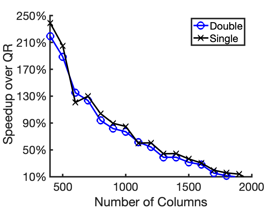
Figure 6. The matrices $\boldsymbol{A}\in{\mathbb{R}}^{m\times n}$ in Figure 6 have $m=10^{5}$ rows, $400\leq n\leq 2000$ columns, condition number $\kappa(\boldsymbol{A})=10^{7}$ and least squares residuals $\|\boldsymbol{A}\boldsymbol{x}_{*}-\boldsymbol{b}\|/(\|\boldsymbol{A}\|\|\boldsymbol{x}_{*}\|)=10^{-6}$. Because the focus of this experiment is about the comparison between single and double precision, we do not estimate the condition number of $\boldsymbol{A}$ and instead specify the precision of the preconditioner in advance. Figure 6(a) shows the average runtime, in seconds, for double precision PNE, mixed precision PNE, and a QR based solver. Figure 6(b) illustrates the speedup of double and mixed precision PNE, computed as the ratio of PNE time over QR solver time.

The mixed precision PNE can be faster than the double precision PNE, as illustrated by $n=400,500,$ and $1000$ columns in Figure 6(b). However, because linear solves dominate the operation count of the PNE over the preconditioner computation, the increase in speed is only modest. Nevertheless, the mixed precision approach offers the complementary benefit of a reduced memory footprint. For $n\leq 2000$ columns, mixed precision and double precision PNE are faster than the QR solver. As the number of columns grows in Figure 6(a), the sketching process becomes more expensive and all three algorithms have similar speed.

Figure 7. The matrices $\boldsymbol{A}\in{\mathbb{R}}^{m\times n}$ in Figure 7 have $m=2^{17}$ rows, $400\leq n\leq 2000$ columns, and least squares residuals $\|\boldsymbol{A}\boldsymbol{x}_{*}-\boldsymbol{b}\|/(\|\boldsymbol{A}\|\|\boldsymbol{x}_{*}\|)=10^{-6}$. In Figure 7(a), $\kappa(\boldsymbol{A})=100$ and in Figure 7(b), $\kappa(\boldsymbol{A})=10^{10}$. Figure 7 shows that the automatic precision selection is accurate for matrices of varying conditioning levels. In Figure 7(a), the half precision preconditioner is almost as accurate as the QR solver for a well conditioned matrix, and the double precision preconditioner in 7(b) is as accurate as the QR solver for an ill conditioned matrix.

(a) $\kappa(\boldsymbol{A})=10^{2}$

(b) $\kappa(\boldsymbol{A})=10^{10}$

Figure 7: Relative errors in the computed solutions $\boldsymbol{\hat{\boldsymbol{x}}}$ and perturbation bounds versus number of columns $n$ for matrices with condition number $\kappa(\boldsymbol{A})=10^{2}$ (Figure 7(a)) and $\kappa(\boldsymbol{A})=10^{10}$ (Figure 7(b)). Shown are the errors in the QR solver (red plusses); the errors from the PNE with an automatic selector for the precision of the preconditoner (blue circles).

References

- [1] H. Avron, P. Maymounkov, and S. Toledo, Blendenpik: supercharging Lapack’s least-squares solver, SIAM J. Sci. Comput., 32 (2010), pp. 1217–1236.
- [2] Å. Björck, Stability analysis of the method of seminormal equations for linear least squares problems, Linear Algebra Appl., 88-89 (1987), pp. 31–48, https://doi.org/https://doi.org/10.1016/0024-3795(87)90101-7.
- [3] J. Burkardt, CONDITION - matrix condition number estimation. https://people.math.sc.edu/Burkardt/cpp_src/condition/condition.html, oct 2012. Accessed: .
- [4] E. Carson and I. Daužickaitė, A comparison of mixed precision iterative refinement approaches for least-squares problems, 2025, https://arxiv.org/abs/2405.18363.
- [5] E. Carson and I. Daužickaitė, Mixed precision sketching for least-squares problems and its application in gmres-based iterative refinement, 2025, https://arxiv.org/abs/2410.06319.
- [6] T. Chen, P. Niroula, A. Ray, P. Subrahmanya, M. Pistoia, and N. Kumar, Gpu-parallelizable randomized sketch-and-precondition for linear regression using sparse sign sketches, 2025, https://arxiv.org/abs/2506.03070.
- [7] E. N. Epperly, M. Meier, and Y. Nakatsukasa, Fast randomized least-squares solvers can be just as accurate and stable as classical direct solvers, 2025, https://arxiv.org/abs/2406.03468.
- [8] J. E. Garrison and I. C. F. Ipsen, A randomized preconditioned Cholesky-QR algorithm, 2024, https://arxiv.org/abs/2406.11751.
- [9] G. H. Golub and C. F. Van Loan, Matrix computations, Johns Hopkins Studies in the Mathematical Sciences, Johns Hopkins University Press, Baltimore, MD, fourth ed., 2013.
- [10] N. J. Higham and S. Pranesh, Exploiting lower precision arithmetic in solving symmetric positive definite linear systems and least squares problems, SIAM Journal on Scientific Computing, 43 (2021), pp. A258–A277, https://doi.org/https://doi.org/10.1137/19M1298263.
- [11] I. C. F. Ipsen, Numerical matrix analysis, Society for Industrial and Applied Mathematics (SIAM), Philadelphia, PA, 2009, https://doi.org/10.1137/1.9780898717686.
- [12] I. C. F. Ipsen, Solution of least squares problems with randomized preconditioned normal equations, 2025, https://arxiv.org/abs/2507.18466.
- [13] I. C. F. Ipsen and T. Wentworth, The effect of coherence on sampling from matrices with orthonormal columns, and preconditioned least squares problems, SIAM J. Matrix Anal. Appl., 35 (2014), pp. 1490–1520.
- [14] L. Lazzarino, Y. Nakatsukasa, and U. Zerbinati, Preconditioned normal equations for solving discretised partial differential equations, 2025, https://arxiv.org/abs/2502.17626.
- [15] H. Li, Double precision is not necessary for LSQR for solving discrete linear ill-posed problems, J. Sci. Comput., 98 (2024), https://doi.org/10.1007/s10915-023-02447-4.
- [16] M. Meier, Y. Nakatsukasa, A. Townsend, and M. Webb, Are sketch-and-precondition least squares solvers numerically stable?, SIAM J. Matrix Anal. Appl., 45 (2024), pp. 905–929, https://doi.org/10.1137/23M1551973.
- [17] J. Papež and P. Tichý, Estimating error norms in CG-like algorithms for least-squares and least-norm problems, Numer. Algorithms, 97 (2024), pp. 1–28, https://doi.org/10.1007/s11075-023-01691-x.
- [18] V. Rokhlin and M. Tygert, A fast randomized algorithm for overdetermined linear least-squares regression, Proc. Natl. Acad. Sci. USA, 105 (2008), pp. 13212–13217.
- [19] J. Scott and M. Tůma, A computational study of low precision incomplete cholesky factorization preconditioners for sparse linear least-squares problems, 2025. arXiv:2504.07580.
- [20] A. Wathen, Some comments on preconditioning for normal equations and least squares, SIAM Rev., 64 (2022), pp. 640–649, https://doi.org/10.1137/20M1387948, https://doi.org/10.1137/20M1387948.
- [21] A. J. Wathen, Least squares and the not-normal equations, SIAM Rev., 67 (2025), pp. 865–872, https://doi.org/10.1137/23M161851X.
- [22] R. Xu and Y. Lu, Randomized iterative solver as iterative refinement: A simple fix towards backward stability, 2024, https://arxiv.org/abs/2410.11115.