Role of $\Xi(1690)$ in the $J/\psi\to\Xi^{0}\bar{\Lambda}K^{0}$ reaction

Abstract

Motivated by the recent BESIII measurements of the $J/\psi\to\Xi^{0}\bar{\Lambda}K_{S}^{0}+c.c.$ process, we investigate this reaction by considering the contributions from the $\Xi(1690)$ and $\Lambda(1890)$ resonances. The $\Xi(1690)$ state is dynamically generated from the $S$-wave pseudoscalar meson-octet baryon interactions within the chiral unitary approach. Our theoretical model provides a good description of the $\bar{\Lambda}K^{0}$, $\Xi^{0}K^{0}$, and $\bar{\Lambda}\Xi^{0}$ invariant mass distributions. The results indicate that the $\Xi(1690)$ resonance, which was neglected in the experimental analysis by BESIII, plays a crucial role in this process. Furthermore, we evaluate the theoretical uncertainties of our model using the parametric bootstrap method. Future high-precision measurements of this process will further help to elucidate the properties of the $\Xi(1690)$ and $\Lambda(1890)$ states.

I Introduction

While the ground-state octet and decuplet baryons have been well established, the spectrum of low-lying excited baryons with spin-parity $J^{P}=1/2^{-}$ remains puzzling. Aside from the well-known $N(1535)$ and $\Lambda(1405)$, the analogous low-lying $\Sigma(1/2^{-})$ and $\Xi(1/2^{-})$ states have not yet been firmly established [1].

Currently, the Review of Particle Physics (RPP) lists two primary candidates for the $\Xi(1/2^{-})$ state [2]. The first is the two-star $\Xi(1620)$, with a mass of approximately 1620 MeV and a width of $(32^{+8}_{-9})$ MeV. The second is the three-star $\Xi(1690)$, with a mass of $(1690\pm 10)$ MeV and a width of $(20\pm 15)$ MeV. However, their spin-parity quantum numbers lack definitive experimental confirmation. Historically, evidence for the $\Xi(1690)^{0}$ was first reported by the Belle and FOCUS Collaborations in 2002 via the resonant contribution in $\Lambda_{c}^{+}\to\Xi(1690)^{0}K^{+}$ [3, 4]. In 2005, the BaBar Collaboration observed the $\Xi(1690)^{0}$ in the $\Lambda_{c}^{+}\to\Lambda\bar{K}^{0}K^{+}$ decay, measuring its mass and width as $(1684.7\pm 1.3(\mathrm{stat})^{+2.2}_{-1.6}(\mathrm{syst}))$ MeV and $(8.1^{+3.9}_{-3.5}(\mathrm{stat})^{+1.0}_{-0.9}(\mathrm{syst}))$ MeV, respectively, and favoring a spin of $J=1/2$ [5]. Subsequent BaBar analyses of $\Lambda_{c}^{+}\to\Xi^{-}\pi^{+}K^{+}$ further supported the $J^{P}=1/2^{-}$ assignment for the $\Xi(1690)$ [6]. More recently, in 2019, the Belle Collaboration reported the first observation of the doubly strange $\Xi(1620)^{0}$ baryon in the $\Xi_{c}^{+}\to\Xi^{-}\pi^{+}\pi^{+}$ process with a significance of $4.0\sigma$ [7], and later identified both the $\Xi(1620)^{0}$ and $\Xi(1690)^{0}$ in the $\Xi\pi$ decay mode from the same process [8].

On the theoretical front, the nature of the $\Xi(1/2^{-})$ states has been extensively explored, though consensus remains elusive. Traditional constituent quark models typically predict the mass of the lowest $\Xi(1/2^{-})$ state to be around 1800 MeV [9, 10, 11, 12], which significantly overestimates the observed masses of both the $\Xi(1620)$ and $\Xi(1690)$. Alternatively, a large-$N_{c}$ QCD approach yields a mass of 1779 MeV [13], while the Skyrme model predicts two distinct $\Xi(1/2^{-})$ states at 1616 MeV and 1658 MeV [14]. Some studies classify the $\Xi(1690)$ as the first orbital excitation with $J^{P}=1/2^{-}$ [15, 16]. Conversely, chiral unitary approaches suggest a molecular picture; in Refs. [19, 18, 17, 20, 21, 22], both the $\Xi(1620)$ and $\Xi(1690)$ emerge dynamically as $J^{P}=1/2^{-}$ resonances generated from the coupled-channel interactions of $\pi\Xi$, $\bar{K}\Lambda$, $\bar{K}\Sigma$, and $\eta\Xi$.

Recently, the BESIII Collaboration analyzed the $J/\psi\to\Xi^{0}\bar{\Lambda}K_{S}^{0}+c.c.$ reaction [23] and determined its branching fraction to be $\mathcal{B}=(3.76\pm 0.14\pm 0.22)\times 10^{-5}$, where the uncertainties are statistical and systematic, respectively. However, the $\bar{\Lambda}K_{S}^{0}$ invariant mass distribution measured by BESIII exhibits a distinct structure around 1.67 GeV (see Fig. 3 of Ref. [23]), which is highly consistent with the mass of the predicted $\Xi(1690)$ state [19, 18, 17].

In the present work, we demonstrate the significant role of the $\Xi(1690)$ in the $J/\psi\to\Xi^{0}\bar{\Lambda}K^{0}$ reaction, where the resonance is dynamically generated from the coupled-channel interactions of $\pi\Xi$, $\bar{K}\Lambda$, $\bar{K}\Sigma$, and $\eta\Xi$. Besides the $\Xi(1690)$ resonance in the $\bar{\Lambda}K^{0}$ channel, the experimental data also exhibits a prominent enhancement near the threshold of the $\Xi^{0}K_{S}^{0}$ invariant mass spectrum. To properly describe these kinematic features, we further incorporate the contribution from the intermediate $\Lambda(1890)$ state. As a well-established baryon with spin-parity $J^{P}=3/2^{+}$, the $\Lambda(1890)$ is known to have a significant coupling to the $\Xi K$ channel. This makes the decay $J/\psi\to\bar{\Lambda}\Lambda(1890)\to\bar{\Lambda}(\Xi^{0}K^{0})$ a natural mechanism to contribute to the observed $\Xi^{0}K^{0}$ distribution. By considering these contributions, we calculate the $\bar{\Lambda}K^{0}$, $\Xi^{0}K^{0}$, and $\bar{\Lambda}\Xi^{0}$ invariant mass distributions. Furthermore, we perform a rigorous analysis of the theoretical uncertainties using the parametric bootstrap method.

This paper is organized as follows. In Sec. II, we present the theoretical formalism for the $J/\psi\to\Xi^{0}\bar{\Lambda}K^{0}$ decay. The numerical results and corresponding discussions are provided in Sec. III. Finally, a brief summary is given in Sec. IV

II Formalism

II.1 Role of $\Xi(1690)$ in $J/\psi\to\Xi^{0}\bar{\Lambda}K^{0}$

In this section, we present the theoretical formalism. We begin with the strong decay process $J/\psi\to\Xi^{0}\bar{\Lambda}K_{S}^{0}$, where the $K_{S}^{0}$ must strictly be a $K^{0}$ due to the nature of the strong decay. It can be seen that the $\bar{\Lambda}K^{0}$ pair can be produced via a $\bar{B}P$ interaction, where $\bar{B}$ is an anti-baryon belonging to the $1/2^{-}$ octet and $P$ is a pseudoscalar meson of the $0^{-}$ octet. To determine which $\bar{B}P$ states are produced in the $J/\psi\to\Xi^{0}\bar{\Lambda}K^{0}$ reaction, we consider the $J/\psi$ to be an SU(3) singlet in the $u,d,s$ sector. By expressing the matrices for the $q\bar{q}$ in terms of mesons with the $\eta$-$\eta^{\prime}$ mixing of Ref. [24], and the $qqq$ and $\bar{q}\bar{q}\bar{q}$ states for the baryon and anti-baryon octets, we have

$$P=\left(\begin{array}[]{ccc}\frac{1}{\sqrt{2}}\pi^{0}+\frac{1}{\sqrt{3}}\eta&\pi^{+}&K^{+}\\[5.69054pt] \pi^{-}&-\frac{1}{\sqrt{2}}\pi^{0}+\frac{1}{\sqrt{3}}\eta&K^{0}\\[5.69054pt] K^{-}&\bar{K}^{0}&~-\frac{1}{\sqrt{3}}\eta\\ \end{array}\right),$$ (4)

$$B=\left(\begin{array}[]{ccc}\frac{1}{\sqrt{2}}\Sigma^{0}+\frac{1}{\sqrt{6}}\Lambda&\Sigma^{+}&p\\[5.69054pt] \Sigma^{-}&-\frac{1}{\sqrt{2}}\Sigma^{0}+\frac{1}{\sqrt{6}}\Lambda&n\\[5.69054pt] \Xi^{-}&\Xi^{0}&~-\frac{2}{\sqrt{6}}\Lambda\\ \end{array}\right),$$ (8)

$$\bar{B}=\left(\begin{array}[]{ccc}\frac{1}{\sqrt{2}}\bar{\Sigma}^{0}+\frac{1}{\sqrt{6}}\bar{\Lambda}&\bar{\Sigma}^{+}&\bar{\Xi}^{+}\\[5.69054pt] \bar{\Sigma}^{-}&-\frac{1}{\sqrt{2}}\bar{\Sigma}^{0}+\frac{1}{\sqrt{6}}\bar{\Lambda}&\bar{\Xi}^{0}\\[5.69054pt] \bar{p}&\bar{n}&~-\frac{2}{\sqrt{6}}\bar{\Lambda}\\ \end{array}\right).$$ (12)

We analyze various SU(3) singlet structures formed by the trace of these products, specifically $\langle\bar{B}BP\rangle$, $\langle\bar{B}PB\rangle$, $\langle\bar{B}B\rangle\langle P\rangle$, $\langle\bar{B}P\rangle\langle B\rangle$, $\langle BP\rangle\langle\bar{B}\rangle$, and $\langle\bar{B}\rangle\langle B\rangle\langle P\rangle$. Among these, terms containing $\langle\bar{B}\rangle$ or $\langle B\rangle$ vanish because $B$ and $\bar{B}$ are traceless matrices. Furthermore, considering that the contribution from the $\langle\bar{B}B\rangle\langle P\rangle$ term is suppressed with respect to single trace structures, as shown using large-$N_{c}$ arguments [25, 26, 27], we focus on the $\langle BP\bar{B}\rangle$ and $\langle B\bar{B}P\rangle$ structures in this study. It is worth noting that we must produce a $\Xi^{0}$ which means we specifically need the $\Xi^{0}P\bar{B}$ and $\Xi^{0}\bar{B}P$ structures. We find

$$\langle BP\bar{B}\rangle\Rightarrow\Xi^{0}\left\{\pi^{-}\bar{\Xi}^{+}-\frac{1}{\sqrt{2}}\pi^{0}\bar{\Xi}^{0}+\frac{1}{\sqrt{3}}\eta\bar{\Xi}^{0}-\frac{2}{\sqrt{6}}K^{0}\bar{\Lambda}\right\},$$ (13)

and

$$\langle B\bar{B}P\rangle\Rightarrow\Xi^{0}\left\{\bar{\Sigma}^{-}K^{+}-\frac{1}{\sqrt{2}}\bar{\Sigma}^{0}K^{0}+\frac{1}{\sqrt{6}}\bar{\Lambda}K^{0}-\frac{1}{\sqrt{3}}\bar{\Xi}^{0}\eta\right\}.$$ (14)

To evaluate these two different structures, $\langle BP\bar{B}\rangle$ and $\langle B\bar{B}P\rangle$, we introduce distinct weights, $A$ and $B$, respectively. Thus, for practical purposes, we have

$$J/\psi\Rightarrow \Xi^{0}\left\{A\left(\pi^{-}\bar{\Xi}^{+}-\frac{1}{\sqrt{2}}\pi^{0}\bar{\Xi}^{0}+\frac{1}{\sqrt{3}}\eta\bar{\Xi}^{0}-\frac{2}{\sqrt{6}}K^{0}\bar{\Lambda}\right)\right.$$

$$\left.+B\left(\bar{\Sigma}^{-}K^{+}-\frac{1}{\sqrt{2}}\bar{\Sigma}^{0}K^{0}+\frac{1}{\sqrt{6}}\bar{\Lambda}K^{0}-\frac{1}{\sqrt{3}}\bar{\Xi}^{0}\eta\right)\right\}.$$ (15)

Since $\Xi^{0}$ has isospin $I=1/2$ and $J/\psi$ $I=0$, the terms in the bracket in Eq. (II.1) will have $I=1/2$. Then, it is convenient to write the expression in bracket in isospin basis, and we take advantage to change the $B$ terms to the meson-baryon order when writing in isospin basis (change of sign for meson-baryon for $I=1/2$, with respect to baryon-meson). Using the isospin multiplets $(\bar{K}^{0},-K^{-})$, $(-\pi^{+},\pi^{0},\pi^{-})$, $(\Xi^{0},-\Xi^{-})$, and $(-\Sigma^{+},\Sigma^{0},\Sigma^{-})$, we obtain

$$\left|\pi\Xi,I=\frac{1}{2},I_{3}=\frac{1}{2}\right>=\sqrt{\frac{2}{3}}\pi^{+}\Xi^{-}-\sqrt{\frac{1}{3}}\pi^{0}\Xi^{0},$$ (16)

$$\left|\bar{K}\Sigma,I=\frac{1}{2},I_{3}=\frac{1}{2}\right>=-\left\{\sqrt{\frac{2}{3}}\Sigma^{+}K^{-}-\sqrt{\frac{1}{3}}\Sigma^{0}\bar{K}^{0}\right\}.$$ (17)

Then the decay to the charge conjugate of Eq. (II.1) can be written as

$$J/\psi\Rightarrow \bar{\Xi}^{0}\left\{\left(\frac{-2A+B}{\sqrt{6}}\right)\bar{K}\Lambda^{I=1/2}+\left(\sqrt{\frac{3}{2}}A\right)\pi\Xi^{I=1/2}\right.$$

$$\left.+\left(-\sqrt{\frac{3}{2}}B\right)\bar{K}\Sigma^{I=1/2}+\left(\frac{A-B}{\sqrt{3}}\right)\eta\Xi^{I=1/2}\right\}.$$ (18)

Figure 1: Mechanisms for tree level $J/\psi\to\Xi^{0}\bar{\Lambda}K^{0}$ and rescattering of intermediate components.

The interaction of the coupled channels leading to the formation of the $\Xi(1690)$ state occurs in the $S$-wave; hence, we keep the $\bar{B}P$ pair in the $S$-wave. However, the $\Xi^{0}\bar{\Lambda}K^{0}$ final state has the spin-parity combination $J^{P}$ of $1/2^{+}$, $1/2^{-}$, and $0^{-}$, resulting in an overall positive parity. Therefore, a $P$-wave is required to match the negative parity of the $J/\psi$. This is achieved by contracting the polarization vector $\epsilon_{\mu}$ of the $J/\psi$ with the momentum of the $\Xi^{0}$. Consequently, as shown in Fig. 1, the transition amplitude for the $J/\psi\to\Xi^{0}\bar{\Lambda}K^{0}$ process is

$$t_{MB}=F\tilde{t}_{MB},$$ (19)

with

$$F=-\epsilon_{\mu}P_{\Xi^{0}}^{\mu},$$ (20)

and

$$\tilde{t}_{MB}= \left\{\frac{-2A+B}{\sqrt{6}}+\frac{-2A+B}{\sqrt{6}}G_{\bar{K}\Lambda}t^{I=1/2}_{\bar{K}\Lambda,\bar{K}\Lambda}\right.$$

$$\left.+\sqrt{\frac{3}{2}}AG_{\pi\Xi}t^{I=1/2}_{\pi\Xi,\bar{K}\Lambda}\right.$$

$$\left.-\sqrt{\frac{3}{2}}BG_{\bar{K}\Sigma}t^{I=1/2}_{\bar{K}\Sigma,\bar{K}\Lambda}\right.$$

$$\left.+\frac{A-B}{\sqrt{3}}G_{\eta\Xi}t^{I=1/2}_{\eta\Xi,\bar{K}\Lambda}\right\},$$ (21)

where we have already used the fact that $t_{M\bar{B},M\bar{B}}=t_{MB,MB}$ since we have at reach the $MB$ amplitudes. For the scattering amplitudes $t_{\bar{K}\Lambda,\bar{K}\Lambda}$, $t_{\pi\Xi,\bar{K}\Lambda}$, $t_{\bar{K}\Sigma,\bar{K}\Lambda}$, and $t_{\eta\Xi,\bar{K}\Lambda}$, we employ the chiral unitary approach with the coupled channels $\pi\Xi$ (1), $\bar{K}\Lambda$ (2), $\bar{K}\Sigma$ (3), and $\eta\Xi$ (4), as described in Refs. [19, 18, 17]. The transition potential is given by

$$V_{ij}= -C_{ij}\frac{1}{4f^{2}}(2\sqrt{s}-M_{i}-M_{j})$$

$$\times\left(\frac{M_{i}+E_{i}}{2M_{i}}\right)^{1/2}\left(\frac{M_{j}+E_{j}}{2M_{j}}\right)^{1/2},$$ (22)

with $f=93$ MeV, where the coefficients are given as,

$$C_{ij}=\begin{pmatrix}2&-\frac{3}{2}&-\frac{1}{2}&0\\[8.0pt] -\frac{3}{2}&0&0&-\frac{3}{2}\\[8.0pt] -\frac{1}{2}&0&2&\frac{3}{2}\\[8.0pt] 0&-\frac{3}{2}&\frac{3}{2}&0\end{pmatrix}.$$ (23)

And the $T$ matrix is given by

$$T=[1-VG]^{-1}V,$$ (24)

where $G_{i}$ is the standard meson-baryon loop function. We regularize it using the cut-off method with $q_{\text{max}}=630$ MeV [19], and the loop function can be written as [28]

$$G_{i}(s)= \frac{2m_{2}}{16\pi^{2}s}\left\{\sigma\left(\arctan\frac{s+\Delta}{\sigma\lambda_{1}}+\arctan\frac{s-\Delta}{\sigma\lambda_{2}}\right)\right.$$ (25)

$$\left.-\left[\left(s+\Delta\right)\ln\frac{q_{\rm max}\left(1+\lambda_{1}\right)}{m_{1}}\right.\right.$$

$$\left.\left.+\left(s-\Delta\right)\ln\frac{q_{\rm max}\left(1+\lambda_{2}\right)}{m_{2}}\right]\right\},$$

where

$$\sigma=\left[-\left(s-(m_{1}+m_{2})^{2}\right)\left(s-(m_{1}-m_{2})^{2}\right)\right]^{1/2},$$ (26)

$$\Delta=m_{1}^{2}-m_{2}^{2},$$ (27)

$$\lambda_{1}=\sqrt{1+\frac{m_{1}^{2}}{q_{\max}^{2}}},~~~~\lambda_{2}=\sqrt{1+\frac{m_{2}^{2}}{q_{\max}^{2}}},$$ (28)

where $m_{1}$ and $m_{2}$ are the mass of meson and baryon, respectively.

II.2 Role of intermediate state $\Lambda(1890)~(3/2^{+})$

Figure 2: Mechanism for intermediate state $\Lambda(1890)$.

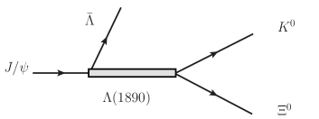
The excitation of the $\Lambda(1890)$ depicted in Fig. 2 relies on a transition between a $1/2^{+}$ and a $3/2^{+}$ baryon state. Similar to the nucleon-$\Delta$ transition, this is achieved through the $S^{\dagger}$ transition spin operator, which is frequently employed in the $\Delta$-hole model for pion nuclear physics [29, 30]. It is defined as [29, 30, 31]

$$\left\langle\frac{3}{2}M\left|S^{\dagger}_{\nu}\right|\frac{1}{2}m\right\rangle=C\left(\frac{1}{2},\mathbf{1},\frac{3}{2};m,\nu,M\right)\left\langle\frac{3}{2}\left|\left|S^{\dagger}\right|\right|\frac{1}{2}\right\rangle,$$ (29)

where $\nu$ is the spherical component of the rank-$\mathbf{1}$ operator $\vec{S}^{\dagger}$, which makes explicit use of the Wigner-Eckart theorem, and the reduced matrix element is defined as 1. For practical calculations, one uses

$$\sum_{M}S_{l}|M\rangle\langle M|S^{\dagger}_{m}=\frac{2}{3}\delta_{lm}-\frac{i}{3}\epsilon_{lms}\sigma_{s},$$ (30)

where $l$, $m$, and $s$ denote Cartesian components. The amplitude for the $\Lambda(1890)$ excitation, featuring a $P$-wave coupling at the $\Lambda(1890)\to K^{0}\Xi^{0}$ transition vertex, is given by [32, 33]

$$\tilde{t}_{\Lambda(1890)}= C\left\langle m^{\prime}\left|S_{i}\tilde{P}_{K^{0}i}\right|M\right\rangle\left\langle M\left|S_{j}^{\dagger}\vec{\epsilon}_{j}\right|m\right\rangle D$$

$$= C\left\langle m^{\prime}\left|\frac{2}{3}\delta_{ij}-\frac{i}{3}\epsilon_{ijs}\sigma_{s}\right|m\right\rangle\tilde{P}_{K^{0}i}\vec{\epsilon}_{j}D,$$ (31)

where

$$D=\dfrac{M_{\Lambda(1890)}}{M_{\text{inv}}(K^{0}\Xi^{0})-M_{\Lambda(1890)}+{i\Gamma_{\Lambda(1890)}}/{2}},$$ (32)

and

$$M_{\Lambda(1890)}=1870~\text{MeV},~~\Gamma_{\Lambda(1890)}=120.0~\text{MeV},$$ (33)

where $\tilde{P}_{K^{0}}$ is the momentum of the $K^{0}$ in the $K^{0}\Xi$ rest frame.

II.3 Full decay amplitude

We can now obtain the full $J/\psi\to\Xi^{0}\bar{\Lambda}K^{0}$ decay amplitude as follows

$$t_{\text{Total}}=t_{1}+t_{2},$$ (34)

with

$$t_{1}=\left(\tilde{t}_{MB}\vec{\epsilon}\cdot\vec{P}_{\Xi^{0}}+C\frac{2}{3}\vec{\epsilon}\cdot\tilde{P}_{K^{0}}D\right),$$ (35)

$$t_{2}=-\frac{i}{3}C\epsilon_{ijs}\sigma_{s}\tilde{P}_{K^{0}i}\vec{\epsilon}_{j}D.$$ (36)

By summing and averaging $|t_{\text{Total}}|^{2}$ over the particle spins, and considering that the $t_{MB}$ amplitudes are spin-independent, we obtain

$$\overline{\sum}\sum|t_{\text{Total}}|^{2} = \frac{2}{3}\left\{\left|\tilde{t}_{MB}\right|^{2}\left|\vec{P}_{\Xi^{0}}\right|^{2}+\frac{2}{3}C^{2}\left|\tilde{P}_{K^{0}}\right|^{2}\left|D\right|^{2}\right.$$ (37)

$$\left.+2\frac{2}{3}\text{Re}\left[\tilde{t}_{MB}\left(CD\right)^{*}\right]\tilde{P}_{K^{0}}\cdot\vec{P}_{\Xi^{0}}\right\},$$

where $\vec{P}_{\Xi^{0}}$ is the momentum of the $\Xi^{0}$ in the $J/\psi$ rest frame, and $\tilde{P}_{K^{0}}$ is the momentum of the $K^{0}$ in the $K^{0}\Xi^{0}$ rest frame, given by

$$\left|\vec{P}_{\Xi^{0}}\right|=\dfrac{\lambda^{1/2}(m_{J/\psi}^{2},M_{\Xi^{0}}^{2},M^{2}_{\text{inv}}(K^{0}\bar{\Lambda}))}{2m_{J/\psi}},$$ (38)

$$\left|\tilde{P}_{K^{0}}\right|=\dfrac{\lambda^{1/2}(M^{2}_{\text{inv}}(K^{0}\Xi^{0}),m_{K^{0}}^{2},M^{2}_{\Xi^{0}})}{2M_{\text{inv}}(K^{0}\Xi^{0})}.$$ (39)

Since $\vec{P}_{\Xi^{0}}$ and $\tilde{P}_{K^{0}}$ are evaluated in different reference frames, we must apply a Lorentz boost. This yields [34]

$$\vec{P}_{\Xi^{0}}=\left[\left(\frac{\tilde{E}_{J/\psi}}{m_{J/\psi}}-1\right)\frac{\tilde{P}_{\Xi^{0}}\cdot\tilde{P}_{J/\psi}}{\tilde{P}_{J/\psi}^{2}}-\frac{\tilde{E}_{\Xi^{0}}}{m_{J/\psi}}\right]\tilde{P}_{J/\psi}+\tilde{P}_{\Xi^{0}},$$ (40)

and where the tilde refers to the $K^{0}\Xi^{0}$ rest frame,

$$\tilde{P}_{K^{0}}=-\tilde{P}_{\Xi^{0}}.$$ (41)

Then, we have

$$\tilde{P}_{K^{0}}\cdot\vec{P}_{\Xi^{0}}= -\left[\left(\frac{\tilde{E}_{J/\psi}}{m_{J/\psi}}-1\right)\frac{\tilde{P}_{\Xi^{0}}\cdot\tilde{P}_{J/\psi}}{\tilde{P}_{J/\psi}^{2}}-\frac{\tilde{E}_{\Xi^{0}}}{m_{J/\psi}}\right]\tilde{P}_{\Xi^{0}}\cdot\tilde{P}_{J/\psi}$$

$$-\left|\tilde{P}_{\Xi^{0}}\right|^{2},$$ (42)

where

$$\tilde{P}_{\Xi^{0}}\cdot\tilde{P}_{J/\psi}=\frac{1}{2}\left\{M_{\Xi^{0}}^{2}+M_{\bar{\Lambda}}^{2}+2\tilde{E}_{\Xi^{0}}\tilde{E}_{\bar{\Lambda}}-M^{2}_{\text{inv}}(\Xi^{0}\bar{\Lambda})\right\},$$ (43)

and

$$\tilde{P}_{J/\psi}=\tilde{P}_{\bar{\Lambda}},$$ (44)

with

$$\left|\tilde{P}_{\bar{\Lambda}}\right|=\dfrac{\lambda^{1/2}(M^{2}_{\text{inv}}(K^{0}\Xi^{0}),M_{\bar{\Lambda}}^{2},m^{2}_{J/\psi})}{2M_{\text{inv}}(K^{0}\Xi^{0})}.$$ (45)

According to the notation 1 to $\Xi^{0}$, 2 to $K^{0}$ and 3 to $\bar{\Lambda}$ and applying the standard kinematics formulas from the RPP [2], we have

$$\dfrac{d^{2}\Gamma}{dM_{12}dM_{23}}=\frac{1}{(2\pi)^{3}}\dfrac{2M_{\bar{\Lambda}}2M_{\Xi^{0}}}{32m_{J/\psi}^{3}}\overline{\sum}\sum|t_{\text{Total}}|^{2}~2M_{12}~2M_{23},$$ (46)

using the Mandl and Shaw normalization for the meson and baryon fields [35].

We can obtain $d\Gamma/dM_{12}$ by integrating $d^{2}\Gamma/(dM_{12}dM_{23})$ over $M_{23}$ within the kinematic limits specified in the RPP [2]. Permuting the indices allows us to evaluate all three invariant mass distributions. We use $M_{12}$ and $M_{23}$ as independent variables, and determine $M_{13}$ using the kinematic relation $M_{12}^{2}+M_{13}^{2}+M_{23}^{2}=m_{J/\psi}^{2}+M_{\Xi^{0}}^{2}+m_{K^{0}}^{2}+M_{\bar{\Lambda}}^{2}$ to get $M_{13}$ from them.

III Results

Figure 3: Invariant mass distributions of $\bar{\Lambda}K^{0}$ (a), $\Xi^{0}K^{0}$ (b), and $\bar{\Lambda}\Xi^{0}$ (c) compared with the BESIII experimental data [23].

Figure 4: Invariant mass distributions of $\bar{\Lambda}K^{0}$ (a), $\Xi^{0}K^{0}$ (b), and $\bar{\Lambda}\Xi^{0}$ (c) compared with the BESIII experimental data [23], obtained from the improved 4-parameter fit which includes the interference phase $\phi$.

Figure 5: Theoretical uncertainties for the invariant mass distributions of $\bar{\Lambda}K^{0}$ (a), $\Xi^{0}K^{0}$ (b), and $\bar{\Lambda}\Xi^{0}$ (c) evaluated using the parametric bootstrap method.

In our model, there are three free parameters: $A$, $B$ and $C$. Fitting these parameters to the experimental data yields $A=-2.49\times 10^{-3}\text{ MeV}^{-2}$, $B=-4.61\times 10^{-4}\text{ MeV}^{-2}$, $C=1.01\times 10^{-4}\text{ MeV}^{-2}$, resulting in a $\chi^{2}/\text{d.o.f.}=444.98/(89-3)=5.17$.

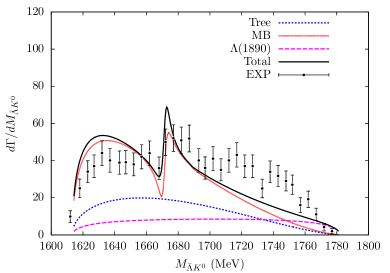
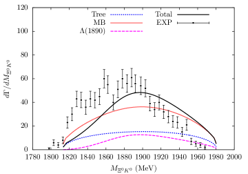
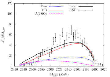
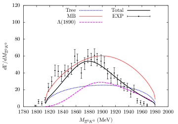
In Fig. 3, we present the invariant mass distributions for $\bar{\Lambda}K^{0}$, $\Xi^{0}K^{0}$, and $\bar{\Lambda}\Xi^{0}$. The blue dotted curves represent the tree-level contributions, while the red dotted curves indicate the contributions from the meson-baryon interaction associated with the $\Xi(1690)$ resonance. Notably, a distinct structure emerges around $1.67\text{ GeV}$ in the $\bar{\Lambda}K^{0}$ invariant mass distribution, which is due to the dynamically generated $\Xi(1690)$ state. The magenta dashed curves display the contribution from the intermediate $\Lambda(1890)(3/2^{+})$ state, and the black solid curves represent the total amplitude. A broad peak is also visible in the $\Xi^{0}K^{0}$ invariant mass distribution. We would like to stress that the singular structure in the region of the $\Xi(1690)$, with a dip followed by a peak, is also present in the experiment. This manifestation of the resonance is similar to the one observed in the $\Xi_{c}^{+}\to\pi^{+}\pi^{+}\Xi^{-}$ [7], which was also reproduced theoretically in Ref. [19]. The shape of the resonance could be different in other reaction, as shown in the study of the $\Xi_{c}^{+}\to\Lambda\bar{K}^{0}\pi^{+}$ in Ref. [21].

To improve the fit, we take advantage of the phase freedom in the $C$ term in Eqs. (35), (36) and (37) by allowing $C$ to acquire a complex phase

$$C\rightarrow Ce^{i\phi}.$$ (47)

With this modification, the model now has four free parameters. The updated fit yields $A=-3.20\times 10^{-3}~\text{MeV}^{-2}$, $B=-5.71\times 10^{-4}~\text{MeV}^{-2}$, $C=-1.53\times 10^{-4}~\text{MeV}^{-2}$, $\phi=0.495\pi$, with a significantly improved $\chi^{2}/\text{d.o.f.}=307.46/(89-4)=3.62$. The corresponding results are displayed in Fig. 4, showing a substantial improvement in reproducing the mass distributions. The theoretical curves are now in fair agreement with the experimental data, successfully capturing the basic kinematic features. Furthermore, the signal of the $\Xi(1690)$ remains distinct.

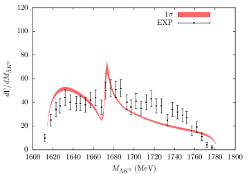
To estimate the theoretical uncertainties and evaluate the model’s sensitivity to the experimental data, we employ a parametric bootstrap (resampling) approach [36, 37, 38]. Specifically, we generate $1000$ sets of pseudo-data by generating new centroids of the data with Gaussian distributions together with the original experimental errors. Our model is then refitted to each of these pseudo-data sets to obtain new sets of parameters and from them the new distributions. These results are presented in Fig. 5, where the bands represent the $1\sigma$ confidence level.

IV Conclusions

Recently, the BESIII Collaboration reported the measurements of the $J/\psi\to\Xi^{0}\bar{\Lambda}K_{S}^{0}+c.c.$ reaction [23]. Notably, the measured $\bar{\Lambda}K_{S}^{0}$ invariant mass distribution reveals a clear structure around 1.67 GeV, which aligns well with the predicted mass of the $\Xi(1690)$ resonance.

Motivated by this observation, we have performed a theoretical study of the $J/\psi\to\Xi^{0}\bar{\Lambda}K^{0}$ process. We specifically focus on the contribution of the $\Xi(1690)$, which is dynamically generated from the $S$-wave coupled-channel interactions of $\pi\Xi$, $\bar{K}\Lambda$, $\bar{K}\Sigma$, and $\eta\Xi$ within the chiral unitary approach. To evaluate the production of the $\Xi(1690)$, we treat the $J/\psi$ as an SU(3) singlet and identify the dominant mechanisms where it decays into an SU(3) octet baryon and a pseudoscalar-baryon pair. Alongside the $\Xi(1690)$, the contribution from the intermediate $\Lambda(1890)$ state is also taken into account.

Particularly, we found that introducing an interference phase between the meson-baryon interaction amplitude and the $\Lambda(1890)$ intermediate state significantly improves the fit quality, successfully capturing the kinematic features of all three invariant mass distributions. Our results yield a satisfactory description of the $\bar{\Lambda}K^{0}$, $\Xi^{0}K^{0}$, and $\bar{\Lambda}\Xi^{0}$ invariant mass distributions simultaneously. This agreement not only supports the molecular nature of the $\Xi(1690)$ but also underscores its indispensable role in this decay process. Given that the properties of the $\Xi(1690)$ are not yet firmly established and the current BESIII data are subject to large statistical uncertainties, future high-precision measurements at facilities like Belle II and the proposed Super Tau-Charm Facility (STCF) will be most welcome. Such experiments will shed further light on the underlying reaction mechanisms and the precise nature of the $\Xi(1690)$.

References

- [1] E. Wang, L. S. Geng, J. J. Wu, J. J. Xie and B. S. Zou, Chin. Phys. Lett. 41, no.10, 101401 (2024)
- [2] S. Navas et al. [Particle Data Group], Phys. Rev. D 110, no.3, 030001 (2024)
- [3] K. Abe et al. [Belle], Phys. Lett. B 524, 33-43 (2002)
- [4] J. M. Link et al. [FOCUS], Phys. Lett. B 624, 22-30 (2005)
- [5] B. Aubert et al. [BaBar], [arXiv:hep-ex/0607043 [hep-ex]].
- [6] B. Aubert et al. [BaBar], Phys. Rev. D 78, 034008 (2008)
- [7] M. Sumihama et al. [Belle], Phys. Rev. Lett. 122, no.7, 072501 (2019)
- [8] M. Sumihama [Belle], AIP Conf. Proc. 2249, no.1, 030040 (2020)
- [9] K. T. Chao, N. Isgur and G. Karl, Phys. Rev. D 23, 155 (1981)
- [10] S. Capstick and N. Isgur, Phys. Rev. D 34, no.9, 2809-2835 (1986)
- [11] L. Y. Glozman and D. O. Riska, Phys. Rept. 268, 263-303 (1996)
- [12] T. Melde, W. Plessas and B. Sengl, Phys. Rev. D 77, 114002 (2008)
- [13] C. L. Schat, J. L. Goity and N. N. Scoccola, Phys. Rev. Lett. 88, 102002 (2002)
- [14] Y. Oh, Phys. Rev. D 75, 074002 (2007)
- [15] M. Pervin and W. Roberts, Phys. Rev. C 77, 025202 (2008)
- [16] L. Y. Xiao and X. H. Zhong, Phys. Rev. D 87, no.9, 094002 (2013)
- [17] K. Miyahara, T. Hyodo, M. Oka, J. Nieves and E. Oset, Phys. Rev. C 95, no.3, 035212 (2017)
- [18] A. Ramos, E. Oset and C. Bennhold, Phys. Rev. Lett. 89, 252001 (2002)
- [19] H. P. Li, G. J. Zhang, W. H. Liang and E. Oset, Eur. Phys. J. C 83, no.10, 954 (2023)
- [20] C. Garcia-Recio, M. F. M. Lutz and J. Nieves, Phys. Lett. B 582, 49-54 (2004)
- [21] Y. Li, W. T. Lyu, G. Y. Wang, L. Li, W. C. Yan and E. Wang, Phys. Rev. D 111, no.5, 054011 (2025)
- [22] S. W. Liu, Q. H. Shen and J. J. Xie, Phys. Rev. D 108, no.11, 114006 (2023)
- [23] M. Ablikim et al. [BESIII], [arXiv:2510.08147 [hep-ex]].
- [24] A. Bramon, A. Grau and G. Pancheri, Phys. Lett. B 283, 416-420 (1992)
- [25] A. V. Manohar, [arXiv:hep-ph/9802419 [hep-ph]].
- [26] L. M. Abreu, L. Dai and E. Oset, Phys. Lett. B 843, 137999 (2023)
- [27] L. R. Dai, W. T. Lyu and E. Oset, [arXiv:2602.09136 [hep-ph]].
- [28] F. K. Guo, R. G. Ping, P. N. Shen, H. C. Chiang and B. S. Zou, Nucl. Phys. A 773, 78-94 (2006)
- [29] T. E. O. Ericson and W. Weise, Clarendon Press, 1988, ISBN 978-0-19-852008-5
- [30] E. Oset, H. Toki and W. Weise, Phys. Rept. 83, 281-380 (1982) doi:10.1016/0370-1573(82)90123-5
- [31] M. Y. Duan, W. T. Lyu, C. W. Xiao, E. Wang, J. J. Xie, D. Y. Chen and E. Oset, Phys. Rev. D 111, no.1, 016004 (2025)
- [32] J. X. Lu, E. Wang, J. J. Xie, L. S. Geng and E. Oset, Phys. Rev. D 93, 094009 (2016)
- [33] H. X. Chen, L. S. Geng, W. H. Liang, E. Oset, E. Wang and J. J. Xie, Phys. Rev. C 93, no.6, 065203 (2016)
- [34] P. Fernández de Córdoba, E. Oset, M. J. Vicente-Vacas, Yu. L. Ratis, J. Nieves, B. López-Alvaredo and F. A. Gareev, Nucl. Phys. A 586, 586-606 (1995)
- [35] F. Mandl and G. Shaw, “QUANTUM FIELD THEORY,”
- [36] M. Albaladejo, D. Jido, J. Nieves and E. Oset, Eur. Phys. J. C 76, no.6, 300 (2016)
- [37] B. Efron and R. Tibshirani, Statist. Sci. 57, no.1, 54-75 (1986)
- [38] W. Press, S. Teukolsky, W. Vetterling, B. Flannery, Numerical recipes in FORTRAN: the art of scientific computing (1992)