Domain Mixture Design via Log-Likelihood Differences
for Aligning Language Models with a Target Model

Abstract

Instead of directly distilling a language model, this study addresses the problem of aligning a base model with a target model in distribution by designing the domain mixture of training data for pretraining or continued pretraining as a fixed training recipe. We propose a method for determining domain weights by viewing models as points in log-likelihood space and aligning the training update direction with the direction toward the target model. Experiments with NanoGPT show that the proposed method consistently reduces the KL divergence to the target model compared with uniform weighting over the Pile. Although knowledge distillation remains more effective when available, the proposed method still achieves meaningful alignment, and downstream task performance also tends to become closer to that of the target model.

Domain Mixture Design via Log-Likelihood Differences
for Aligning Language Models with a Target Model

Ryo Kishino¹   Riku Shiomi¹   Hiroaki Yamagiwa¹ Momose Oyama^1,2   Hidetoshi Shimodaira^{1,2 1}Kyoto University ²RIKEN {kishino.ryo.32s, shiomi.riku.52p}@st.kyoto-u.ac.jp, oyama.momose@sys.i.kyoto-u.ac.jp, {h.yamagiwa, shimo}@i.kyoto-u.ac.jp

1 Introduction

The properties of large language models depend not only on their architecture and model size but also on the distribution of text used for training Albalak et al. (2024). In particular, large-scale corpora such as the Pile Gao et al. (2021) consist of multiple domains, and the mixture weights over these domains strongly affect model behavior Xie et al. (2023). Therefore, designing the domain mixture of the training data is an important problem for enabling models to acquire desired properties.

In this study, we address the problem of determining the training text distribution for updating a base model so as to align it with a target model in distribution. A common approach is to directly imitate the target model through knowledge distillation Hinton et al. (2015) or by training on text generated by the target model Kim and Rush (2016). However, such methods require access to the teacher model and incur additional generation or inference costs. Moreover, even when the domain weights used in prior training are known, simply reusing them is not necessarily optimal in the current setting. We therefore aim to achieve model alignment by designing the domain weights of the training text as a fixed training recipe specified before training begins. The estimated domain weights can serve not only as a target-informed starting point for further training under different settings, but also as an interpretable summary of the domain-level shift from the base model toward the target.

Figure 1: t-SNE visualization of training trajectories in the log-likelihood vector space during continued pretraining from pretrained NanoGPT toward Gemma-2B. The trajectories are obtained using either uniform domain weights over the Pile domains or weights determined by the proposed method (aggregated-LLD). Each point represents a checkpoint taken every 1k training steps, and color intensity indicates the number of training steps. The star denotes the target model. Compared with uniform weighting, the proposed method yields a trajectory that moves more consistently toward the target model. See Section 4.3 for details.

We represent a model as a vector of mean log-likelihoods over multiple text collections Oyama et al. (2025). In this study, we use the domains of the Pile Gao et al. (2021) as these text collections. Directly comparing different models in parameter space is difficult because of architectural mismatches and permutation symmetries of network weights induced by hidden-unit reordering Hecht-Nielsen (1990). In contrast, mean log-likelihood vectors computed on a set of text collections provide a common basis for comparison across models. With this representation, model alignment can be viewed as a geometric problem of moving the base model toward the target model, leading to a rule for determining mixture proportions based on the domain-level log-likelihood differences (LLD) between the target and base models.

In experiments using NanoGPT as the base model, determining the domain weights for the Pile using the proposed method consistently reduces the KL divergence to either Gemma-2B or CodeGemma-2B compared with training using uniform weights (see Fig. 1). For target models that share the same tokenizer, the proposed method provides a useful alternative to knowledge distillation, although distillation remains more effective when available.

2 Background and Related Work

2.1 Data selection and mixing for LLMs

Selecting and mixing training data has become an important issue in LLM training, as performance depends not only on the amount of data but also on its distribution Albalak et al. (2024). In particular, for multi-domain corpora such as the Pile Gao et al. (2021), the choice of domain weights substantially affects model properties and can lead to markedly different training trajectories in log-likelihood space (Fig. 2). This has led to active research on optimizing training data selection and domain weights for downstream tasks, domain adaptation, and training efficiency Zhou et al. (2023); Xie et al. (2023); Ye et al. (2025); Liu et al. (2024); Dohmatob et al. (2025).

As a classical data selection method, Moore and Lewis (2010) proposed ranking texts in a general-domain corpus based on the log-likelihood difference between a language model trained on the target domain and another trained on the general domain. Like this method, our study uses log-likelihood differences between two models on text. The two approaches differ in three important respects: our method estimates domain weights rather than selecting texts, aims to align the base model with the target model in distribution, and derives a rule for determining domain weights from a geometric perspective in log-likelihood space.

Recently, there has also been growing interest in directly optimizing domain weights. Xie et al. (2023) estimated the difficulty of each domain based on the log-likelihoods of a small model and determined the domain weights for pretraining a larger model. Liu et al. (2024), in a knowledge distillation setting, dynamically updated the domain weights of the distillation data according to the domain-level likelihood ratios between the teacher and the student. In contrast, our study aims to align a base model with a specific target model by designing domain weights as a fixed training recipe, without using distillation. Our study can therefore be viewed as distillation-free data mixture design for distributional alignment to a target model.

Figure 2: t-SNE visualization of NanoGPT training trajectories for two training datasets independently sampled from each of two domain mixtures over the Pile. Each point represents a checkpoint taken every 1k training steps, and color intensity indicates the number of training steps. Differences in trajectory are much larger across domain mixtures than across datasets sampled from the same mixture. The two mixtures are obtained by doubling the weights of either the code-related domains or the PubMed-related domains relative to the original Pile weights. See Appendix B for details.

2.2 Log-likelihood vector

As a framework for comparing models in a shared space, Oyama et al. (2025) introduced, for a language model $p$, the text-level log-likelihood vector over a set of $N$ texts $\mathcal{D}=\{x_{1},\ldots,x_{N}\}$,

$$\bm{\ell}^{\text{text}}=(\log p(x_{1}),\ldots,\log p(x_{N}))^{\top}\in\mathbb{R}^{N},$$ (1)

which serves as a representation of $p$. For $M$ models (or checkpoints along a training trajectory) $p_{1},\ldots,p_{M}$, let

$$\bm{L}=(\bm{\ell}^{\text{text}}_{1},\ldots,\bm{\ell}^{\text{text}}_{M})^{\top}\in\mathbb{R}^{M\times N}$$

and define

$$\bm{Q}=(\bm{q}_{1},\ldots,\bm{q}_{M})^{\top}\in\mathbb{R}^{M\times N}$$

as the matrix obtained by double-centering $\bm{L}$. Then, the KL divergence between $p_{i}$ and $p_{j}$ is approximated as

$$2\operatorname{KL}(p_{i},p_{j})\approx\|\bm{q}_{i}-\bm{q}_{j}\|^{2}/N.$$ (2)

This approximation enables comparison of models with different architectures in a shared geometric space. Moreover, log-likelihood vectors have been shown to be useful for predicting downstream task performance. They have also been applied to the analysis of training trajectories during pretraining Kishino et al. (2026) and to the analysis of how training data contributes to learning efficiency Harada et al. (2025); Aoki et al. (2025).

Building on this framework, we use the text-level log-likelihood vector to analyze training trajectories and the domain-level log-likelihood vector, consisting of mean log-likelihoods for each domain, to design domain weights for training.

3 Method

In this study, we consider domain weights for aligning a base model with a target model in log-likelihood space. Our main objective is to design a single set of domain weights fixed once before training. We first formulate the problem and derive a theoretical criterion that determines domain weights iteratively based on update-direction alignment as a first pass. We then aggregate the resulting weights into a form that is easier to use as a fixed recipe in a second pass.

3.1 Text distribution

For each domain $k\in\{1,\ldots,K\}$, let $r_{k}(x)$ denote the domain-specific text distribution. Let

$$\bm{\pi}=(\pi_{1},\ldots,\pi_{K})^{\top}\in\Delta^{K-1}$$

denote the domain weights, where

$$\Delta^{K-1}=\left\{\bm{\pi}:\sum_{k=1}^{K}\pi_{k}=1,\ \pi_{k}\geq 0\right\}$$

is the $(K-1)$-dimensional probability simplex. We then define the corresponding mixture text distribution as

$$r_{\bm{\pi}}(x)=\sum_{k=1}^{K}\pi_{k}r_{k}(x).$$

3.2 Domain-level log-likelihood vector

For each $k$, let $\mathcal{D}_{k}$ denote a set of texts sampled from $r_{k}$, and let

$$\mathcal{D}=\bigcup_{k=1}^{K}\mathcal{D}_{k}$$

be the union of these sets. We refer to $\mathcal{D}$ as the evaluation corpus.

We consider a base model $p_{\bm{\theta}}(x)$ and a target model $p_{\text{tgt}}(x)$, where $\bm{\theta}\in\mathbb{R}^{P}$ denotes the parameters of the base model. The goal of this study is to align the base model with the target model through pretraining or continued pretraining. The two models need not share the same architecture.

For the base model $p_{\bm{\theta}}(x)$, we define the domain-level log-likelihood vector on the evaluation corpus $\mathcal{D}$ by

$${\bm{\ell}}(\bm{\theta})=\begin{pmatrix}\frac{1}{|\mathcal{D}_{1}|}\sum_{x\in\mathcal{D}_{1}}\log p_{\bm{\theta}}(x)\\ \vdots\\ \frac{1}{|\mathcal{D}_{K}|}\sum_{x\in\mathcal{D}_{K}}\log p_{\bm{\theta}}(x)\end{pmatrix}\in\mathbb{R}^{K}.$$ (3)

Similarly, let $\bm{\ell}_{\text{tgt}}\in\mathbb{R}^{K}$ denote the domain-level log-likelihood vector for the target model $p_{\text{tgt}}(x)$.

3.3 Derivation of a rule for determining domain weights

Figure 3: Illustration of the update direction in log-likelihood space when the base model $p_{\bm{\theta}}$ is updated along the gradient direction in parameter space using a text sampled from the mixture distribution $r_{\bm{\pi}}$. Our goal is to estimate $\bm{\pi}$ so that the blue update direction aligns with the red direction toward the target model.

We first derive how training changes the log-likelihood vector. Assuming SGD with learning rate $\eta>0$, the parameter update with a text $x\sim r_{\bm{\pi}}$ is given by

$$\Delta\bm{\theta}:=\eta\nabla_{\bm{\theta}}\log p_{\bm{\theta}}(x),\quad\bm{\theta}\leftarrow\bm{\theta}+\Delta\bm{\theta}.$$

Let the domain-level Jacobian on the evaluation corpus be

$${\bm{J}}(\bm{\theta})=\nabla_{\bm{\theta}}{\bm{\ell}}(\bm{\theta})^{\top}\in\mathbb{R}^{P\times K}.$$

Then, the expected change in the log-likelihood vector is approximated as

$$\mathbb{E}_{x\sim r_{\bm{\pi}}}[{\bm{\ell}}(\bm{\theta}+\Delta\bm{\theta})-{\bm{\ell}}(\bm{\theta})]\approx{\eta}{\bm{J}}(\bm{\theta})^{\top}{\bm{J}}(\bm{\theta})\bm{\pi}.$$ (4)

See Appendix A.1 for the proof.

For simplicity, we omit the explicit dependence on $\bm{\theta}$ and write $\bm{\ell}$ and $\bm{J}$. We refer to $\bm{J}^{\top}\bm{J}$ as the Gram matrix. Equation (4) implies that the expected update direction in log-likelihood space is approximated by $\eta{\bm{J}}^{\top}{\bm{J}}\bm{\pi}$, shown as the blue arrow in Fig. 3. Our goal is to align this direction with the target direction ${\bm{\ell}}_{\text{tgt}}-{\bm{\ell}}$, shown as the red arrow.

If we ignore the constraint $\bm{\pi}\in\Delta^{K-1}$, we seek $\bm{\pi}$ such that the expected update direction matches the target direction:

$${\bm{J}}^{\top}{\bm{J}}\bm{\pi}={\bm{\ell}}_{\text{tgt}}-{\bm{\ell}}.$$

The unconstrained weight vector satisfying this relation is

$$\tilde{\bm{\pi}}=({\bm{J}}^{\top}{\bm{J}})^{-1}({\bm{\ell}}_{\text{tgt}}-{\bm{\ell}}).$$

To obtain domain weights in $\Delta^{K-1}$, we consider the optimization problem

$$\max_{\bm{\pi}\in\Delta^{K-1}}~\bm{\pi}^{\top}\tilde{\bm{\pi}}-\tau\operatorname{KL}(\bm{\pi},\mathrm{unif}).$$ (5)

Here, $\tau>0$ is the temperature parameter controlling the strength of regularization, and $\operatorname{KL}(\bm{\pi},\mathrm{unif})$ is a regularization term that encourages domain weights close to the uniform weights $\mathrm{unif}=(1/K,\ldots,1/K)^{\top}$, thereby avoiding extreme weights. The solution to (5) is the softmax of $\tilde{\bm{\pi}}/\tau$:

$$\pi_{k}=\frac{\exp(\tilde{\pi}_{k}/\tau)}{\sum_{k^{\prime}=1}^{K}\exp(\tilde{\pi}_{k^{\prime}}/\tau)}.$$ (6)

The proof is given in Appendix A.2.

In practice, computing the Gram matrix $\bm{J}^{\top}\bm{J}$ requires $O(K^{2}P)$ time, which imposes substantial computational and memory costs for large language models with a huge number of parameters $P$. We therefore omit $({\bm{J}}^{\top}{\bm{J}})^{-1}$, which provides sensitivity adjustment across domains, and instead use a heuristic approximation given by the softmax of $({\bm{\ell}}_{\text{tgt}}-{\bm{\ell}})/\tau$:

$$\pi_{k}=\frac{\exp(({\ell}_{\mathrm{tgt},k}-{\ell}_{k})/\tau)}{\sum_{k^{\prime}=1}^{K}\exp(({\ell}_{\mathrm{tgt},k^{\prime}}-{\ell}_{k^{\prime}})/\tau)}.$$ (7)

In what follows, we use this approximation as a practical mixture design method, while treating the method with the adjustment matrix $({\bm{J}}^{\top}{\bm{J}})^{-1}$ as a theoretical reference method.

3.4 Iterative estimation of domain weights and aggregation

As (7) indicates, the domain weights depend on ${\bm{\ell}}(\bm{\theta})$, so the theoretically desirable weights change during training. We therefore adopt a two-pass procedure. In the first pass, the domain weights are computed at selected update steps and then aggregated into a single set of weights, $\bm{\pi}^{*}$, to be used as a fixed training recipe. In the second pass, the model is trained using $\bm{\pi}^{*}$, without further reference to the target model.

Here, $\mathcal{D}$ denotes the evaluation corpus used to compute the domain-level log-likelihood vector, and $\mathcal{C}_{k}$ denotes the training corpus for domain $k$. Let

$$\mathcal{T}=\{t_{1},\ldots,t_{|\mathcal{T}|}\}$$

denote the set of training steps at which domain weights are estimated. Given domain weights $\bm{\pi}^{(t)}$ at step $t$, we define the fixed domain weights $\bm{\pi}^{*}$ by geometric-mean aggregation over $t\in\mathcal{T}$:

$$\pi_{k}^{*}\propto\left(\prod_{t\in\mathcal{T}}\pi_{k}^{(t)}\right)^{1/|\mathcal{T}|}.$$ (8)

This coincides with the point in $\Delta^{K-1}$ that minimizes the sum of KL divergences to $\bm{\pi}^{(t)}$:

$$\bm{\pi}^{*}=\operatorname*{arg\,min}_{\bm{\pi}\in\Delta^{K-1}}\sum_{t\in\mathcal{T}}\operatorname{KL}(\bm{\pi},\bm{\pi}^{(t)}).$$ (9)

See Appendix A.4 for the proof.

We call adjusted-LLD the theoretical reference method that updates domain weights at each step in $\mathcal{T}$ according to (6), using the sensitivity adjustment $(\bm{J}^{\top}\bm{J})^{-1}$. In contrast, we call iterative-LLD the method that updates domain weights at each step according to (7) without the sensitivity adjustment. We call aggregated-LLD the two-pass method that aggregates the iterative-LLD weights over the steps in $\mathcal{T}$ via (8) to estimate fixed domain weights $\bm{\pi}^{*}$, and then trains the base model using them. Algorithm 1 summarizes the first pass.

Algorithm 1 First-pass estimation of the fixed domain weights $\bm{\pi}^{*}$ for aggregated-LLD

1:base model $p_{\bm{\theta}}$, target model $p_{\text{tgt}}$, evaluation corpus $\mathcal{D}$, domain-specific training corpora $\{\mathcal{C}_{k}\}_{k=1}^{K}$, update steps $\mathcal{T}$, total training steps $t_{\text{max}}$, temperature $\tau$

2:domain weights $\bm{\pi}^{*}$

3:

4:Compute the domain-level log-likelihood vector ${\bm{\ell}}_{\text{tgt}}$ using (3)

5:for $t=0,\ldots,t_{\text{max}}$ do

6:  if $t\in\mathcal{T}$ or $t=0$ then

7:   Compute ${\bm{\ell}}(\bm{\theta})$ using (3)

8:   Estimate $\bm{\pi}^{(t)}$ using (7)

9:  else

10:   Set $\bm{\pi}^{(t)}\leftarrow\bm{\pi}^{(t-1)}$

11:  end if

12:  Sample a domain $k$ according to the domain weights $\bm{\pi}^{(t)}$

13:  Update $\bm{\theta}$ using a batch sampled from $\mathcal{C}_{k}$

14:end for

15:Aggregate $\{\bm{\pi}^{(t)}\}_{t\in\mathcal{T}}$ using (8) to obtain $\bm{\pi}^{*}$

4 Experiments

In this section, we evaluate how well alignment with the target model can be achieved by training the base model using domain weights designed by the proposed method. We examine five aspects: (i) the validity of domain-weight estimation for target models with known domain weights, (ii) alignment with publicly available LLMs, (iii) comparison with knowledge distillation, (iv) ablation on the softmax temperature $\tau$ used to estimate domain weights, and (v) similarity in downstream task performance. Details of the experimental setup are provided in Appendix B.

4.1 Experimental setup

Datasets.

Both the evaluation and training texts are taken from the Pile Uncopyrighted, which contains $K=17$ domains. For the evaluation corpus $\mathcal{D}$ used for computing log-likelihood vectors, we use the same 10,000 texts as in Oyama et al. (2025). These texts are chunked into 1024-byte segments, and KL divergence is measured on this text set in bits per byte using (2). By contrast, each domain corpus $\mathcal{C}_{k}$ used to train the base model is also derived from the Pile Uncopyrighted, but consists of original texts tokenized and stored separately by domain. During training, each batch is constructed from a domain sampled according to the domain weights. The total number of tokens per training step is $2^{19}\approx 500\mathrm{k}$.

Base/target model settings.

In our experiments, we use NanoGPT Karpathy (2022) with 124M parameters as the base model. To examine whether the proposed method remains effective even when the base model has already acquired general knowledge, we consider not only a randomly initialized NanoGPT but also a NanoGPT pretrained on FineWeb 100BT Penedo et al. (2024). As target models, we use publicly available models such as Gemma-2B gemmateam2024gemmaopenmodelsbased and CodeGemma-2B codegemmateam2024codegemmaopencodemodels, as well as NanoGPT pretrained on the Pile with controlled domain weights. In particular, we define CodeNanoGPT as a model trained for 100k steps on the Pile with the weights of GitHub, Stack Exchange, Ubuntu IRC, and Hacker News doubled relative to their original values, increasing the total proportion of code-related domains from 18.9% to 37.9%. See Appendix B for the hyperparameters used in these pretraining runs.

Computation of the domain-level log-likelihood vector.

The domain-specific corpus $\mathcal{C}_{k}$ used for training and the evaluation text set $\mathcal{D}$ differ in how texts are segmented. The text sequences used to construct training batches have a fixed token length, whereas the evaluation texts vary in token length, as shown in Table 3 in Appendix B. To make log-likelihoods from the two settings comparable, we normalize the domain-level mean log-likelihoods in (3) by the mean token length of each domain.

Figure 4: Comparison of domain weights estimated by aggregated-LLD and uniform weights against the ground-truth. The target model is CodeNanoGPT, pretrained with known domain weights, and the base model is a randomly initialized NanoGPT. The KL values in the legend denote the KL divergence from the ground-truth domain weights.

Base model training.

The base model is trained for 10k steps in both pretraining and continued pretraining. The first 1k steps serve as a warmup period, after which the learning rate is cosine-decayed from 6e-4 to 6e-5. At each step, one domain is sampled according to the domain weights, and the batch is constructed from that domain. The domain weights are updated iteratively at steps 0, 1, 2, 4, 8, 16, 32, 64, 128, 256, 512, 1k, 2k, …, 9k. This follows the Pythia setting Biderman et al. (2023), in which checkpoints are saved densely during the warmup. For iterative-LLD and adjusted-LLD, training proceeds while iteratively estimating domain weights at these steps using the current base model. In contrast, for aggregated-LLD, we first aggregate the domain weights obtained by iterative-LLD to determine a fixed set of domain weights, and then train the base model using these fixed domain weights. Unless otherwise noted, the softmax temperature in (7) for domain-weight estimation is set to $\tau=1$. Although the proposed method is derived under a first-order approximation based on SGD for simplicity, the experiments use AdamW Loshchilov and Hutter (2019), which is widely used in practice. Our goal is therefore not to claim exact agreement between the theory and the actual training dynamics, but to evaluate whether the derivation is effective as a practical rule for designing domain weights.

4.2 Comparison with ground-truth weights

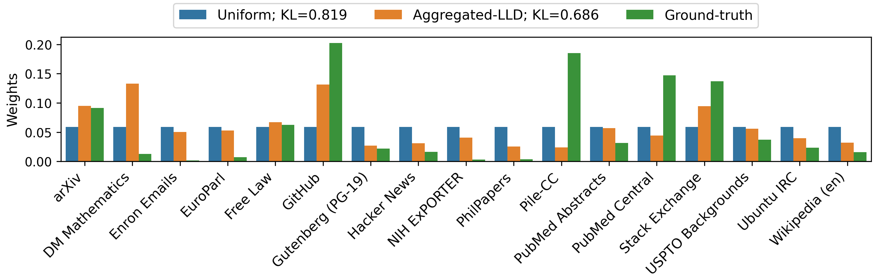
To examine how aggregated-LLD estimates domain weights, we consider a setting in which the target model is CodeNanoGPT, whose ground-truth weights are known, and the base model is a randomly initialized NanoGPT. Fig. 4 shows the domain weights $\bm{\pi}^{*}$ estimated by Algorithm 1.

The KL divergence from the ground-truth domain weights is 0.819 for uniform weights and 0.686 for the estimated weights. This indicates that the proposed method yields domain weights closer to the ground-truth than uniform weights. In particular, for code-related domains whose weights are increased in the ground-truth, such as GitHub and Stack Exchange, the estimated weights are broadly consistent with the ground-truth trend. Although the estimated weights do not exactly match the ground-truth, they capture the target model’s overall domain weighting pattern.

4.3 Distributional alignment via estimated domain weights

We evaluate how much the KL divergence to the target model is reduced when the base model is trained with the estimated domain weights. We compare uniform domain weights, adjusted-LLD, iterative-LLD, and aggregated-LLD.

We use Gemma-2B and CodeGemma-2B as target models, and random-init or pretrained NanoGPT as base models. Figs. 5(a) and 5(b) show KL divergence over training steps, and Table 1 reports final-step KL divergence. Overall, LLD-based domain weights achieve lower KL divergence than uniform domain weights in all settings.

Among the three methods, adjusted-LLD serves as the theoretical reference method and indeed achieves the smallest KL divergence in all settings. Although iterative-LLD and aggregated-LLD do not reach adjusted-LLD, both outperform uniform domain weights in all settings. Moreover, the difference between iterative-LLD and aggregated-LLD is small. Therefore, aggregated-LLD has a practical advantage: it provides fixed domain weights set before training while maintaining performance close to iterative-LLD. We discuss the stability of the weights estimated by iterative-LLD in Appendix C.

Fig. 1 visualizes, using t-SNE van der Maaten and Hinton (2008), the training checkpoints of pretrained NanoGPT in the $\bm{q}$-coordinates obtained by double-centering text-level log-likelihood vectors on the evaluation corpus, following Oyama et al. (2025). By (2), the squared Euclidean distance in this space approximates the KL divergence between models. The figure shows that training with the domain weights estimated by aggregated-LLD moves closer to the target model than training with uniform weights.

(a) Target model: Gemma-2B.

(b) Target model: CodeGemma-2B.

Figure 5: KL divergence to the target model over training steps when random-init/pretrained NanoGPT is trained with different domain weights.

Target	Method	Base
		random-init	pretrained
Gemma-2B	uniform	18.1	12.0
	aggregated-LLD	16.9	11.0
	iterative-LLD	16.0	10.8
	adjusted-LLD	13.5	9.26
CodeGemma-2B	uniform	26.7	22.9
	aggregated-LLD	21.4	18.2
	iterative-LLD	21.0	18.6
	adjusted-LLD	14.8	14.5

Table 1: Final-step KL divergence (bits/byte) to the target model for random-init/pretrained NanoGPT trained with different domain weights.

Analysis of $({\bm{J}}^{\top}{\bm{J}})^{-1}$.

Fig. 6 shows the absolute values of the entries of the adjustment matrix $({\bm{J}}^{\top}{\bm{J}})^{-1}$ for random-init and pretrained NanoGPT, computed on the evaluation corpus $\mathcal{D}$ at step $t=0$. In both cases, the diagonal entries are relatively large, indicating that the adjustment is dominated by each domain’s own component. This is consistent with the practical effectiveness of LLD without explicit sensitivity adjustment in (7). For pretrained NanoGPT, however, several off-diagonal entries are also non-negligible, including those between GitHub and Stack Exchange and between Pile-CC and Wikipedia (en). Correcting for such inter-domain correlations may help explain the stronger performance of adjusted-LLD.

Figure 6: Heatmaps of the absolute values of the entries of the adjustment matrix $({\bm{J}}^{\top}{\bm{J}})^{-1}$ for random-init and pretrained NanoGPT. Rows and columns correspond to domains in the Pile.

4.4 Comparison with knowledge distillation

Figure 7: KL divergence to the target model, CodeNanoGPT, over training steps for random-init and pretrained NanoGPT trained with uniform domain weights, domain weights estimated by aggregated-LLD, or distillation.

We compare aggregated-LLD with knowledge distillation. We use CodeNanoGPT as the target model so that the base model and the target model share the same tokenizer. For distillation, we use uniform domain weights and consider two objectives: KL divergence alone, and the sum of KL divergence and the cross-entropy loss. Although optimizing domain weights for distillation could yield further improvements Liu et al. (2024), we adopt this simplest setting to make the comparison with the proposed method clearer.

The results are shown in Fig. 7. When random-init NanoGPT is used as the base model, the KL divergence from the target model at the final training step is 4.39, 4.07, 2.65, and 2.13 bits/byte for uniform, aggregated-LLD, distill w/o CE, and distill w/ CE, respectively. When pretrained NanoGPT is used as the base model, the corresponding values are 2.59, 1.96, 1.56, and 0.99 bits/byte. Although knowledge distillation achieves the smallest KL divergence, aggregated-LLD consistently outperforms the uniform setting. These results suggest that, while the proposed method is not intended to replace distillation, it can achieve a meaningful degree of distributional alignment under weaker supervision using only pre-estimated domain weights. The proposed method is therefore a useful alternative in settings where distillation is not feasible.

4.5 Ablation on temperature

Base	$\tau=0.1$	$\tau=1.0$	$\tau=10$	$\tau=\infty$*
Random-init	5.83	4.07	4.35	4.39
Pretrained	6.22	1.96	2.48	2.59

^* $\tau=\infty$ corresponds to the uniform weights.

Table 2: KL divergence (bits/byte) to the target model, CodeNanoGPT, under different values of $\tau$.

The temperature $\tau$ in (7) controls the sharpness of the estimated domain weights. In this section, we examine the effect of $\tau\in\{0.1,1.0,10,\infty\}$ using random-init or pretrained NanoGPT as the base model and CodeNanoGPT as the target model, where $\tau=\infty$ corresponds to uniform weights. As shown in Table 2, when trained with aggregated-LLD, the KL divergence at the final training step from the target model is minimized at $\tau=1.0$ for both random-init and pretrained NanoGPT.

A low softmax temperature concentrates the domain weights on a few domains, whereas a high temperature makes them closer to uniform. The difference in mean log-likelihood per token between random-init NanoGPT and CodeNanoGPT ranged from 7.3 (Pile-CC) to 9.1 (DM Mathematics), giving a spread of 1.8. Choosing a temperature on the same scale as this range helps avoid extreme outcomes.

4.6 Alignment in task performance

Figure 8: (Top) Comparison of the target model and the final checkpoint trained with aggregated-LLD on five tasks. (Bottom) Across checkpoints at different training steps, the relationship between the KL divergence to the target model and the Pearson correlation of the five-task performance profiles.

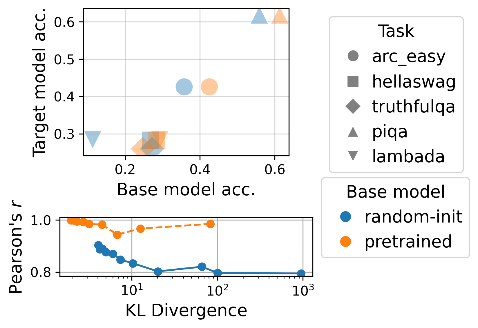
We examine whether bringing a model closer to the target model in log-likelihood space using the proposed method also makes its downstream performance profile closer to that of the target model.

We use random-init and FineWeb-pretrained NanoGPT as the base models and CodeNanoGPT as the target model. For evaluation, we use AI2 Reasoning Challenge (ARC) Clark et al. (2018), HellaSwag Zellers et al. (2019), TruthfulQA Lin et al. (2022), PIQA Bisk et al. (2020), and LAMBADA Paperno et al. (2016). All evaluations are conducted using lm-evaluation-harness Gao et al. (2024).

As shown in Fig. 8, the final checkpoint trained with aggregated-LLD exhibits task performance that generally corresponds to that of the target model across downstream tasks. Moreover, as the KL divergence to the target model decreases, the Pearson correlation between the performance vectors also tends to increase.

5 Conclusion

We proposed a method for aligning a base model with a target model during pretraining or continued pretraining by controlling domain weights in the training data. Using a geometric formulation in log-likelihood space, we derived a theoretical criterion for domain weights that steer the update direction toward the target model and approximated it with fixed domain weights. Experiments with NanoGPT showed that the proposed method yields smaller KL divergence than uniform domain weights and brings the base model meaningfully closer to the target model. For target models that share the same tokenizer, the proposed method provides a useful alternative to knowledge distillation, although knowledge distillation remains more effective when available. As KL divergence decreases, downstream task performance also tends to become closer to that of the target model.

Limitations

• Our experiments are conducted primarily using NanoGPT with 124M parameters. Whether the same behavior also holds for substantially larger models, such as those with several billion parameters or more, has not been examined due to computational resource constraints and remains future work.

• We primarily evaluate our method on specific pretrained models. Its generality to a broader range of architectures, as well as to models that have undergone instruction tuning or alignment through reinforcement learning, has not yet been sufficiently examined.

• This study assumes the Pile Uncopyrighted and thus relies on a large-scale corpus with explicitly defined domains. It remains unverified whether the same optimization of domain weights is effective for other corpora or for datasets with ambiguous domain boundaries. In particular, the results may vary substantially depending on the granularity of the domain partitioning. Extending the method to finer granularities, such as sentence-level units, to pseudo-domains obtained by clustering in embedding space, or to settings in which a text belongs to multiple domains remains important future work.

• As described in Section 4.1 and Appendix B, the evaluation text set $\mathcal{D}$ is the same as that used by Oyama et al. (2025) and therefore consists of texts with variable token lengths. Since actual training is performed with a fixed token length, we normalize the log-likelihood by token length for each domain. Ideally, such normalization would be unnecessary if a fixed-token-length evaluation set were used from the outset. At the same time, allowing variable-length texts is itself natural when users may evaluate models on arbitrary text sets. The effect of this particular choice of $\mathcal{D}$ on the results has not been examined.

• For simplicity, the theory assumes SGD as the training algorithm, whereas the experiments use AdamW, which is widely adopted in practice. Although we empirically confirm the alignment effect in this study, the exact correspondence between the internal dynamics of AdamW and the geometric interpretation in log-likelihood space remains unclear.

• Adjusted-LLD uses the adjustment matrix $(\bm{J}^{\top}\bm{J})^{-1}$, but computing it requires $O(K^{2}P)$ time, making both the computational and memory costs substantial for large language models. For this reason, we treat the criterion based on $(\bm{J}^{\top}\bm{J})^{-1}$ as a theoretical reference method and primarily use its approximations, iterative-LLD and aggregated-LLD, in our experiments. Since what is actually required is the Gram matrix $\bm{J}^{\top}\bm{J}$ rather than the Jacobian itself, approximate computation via partial parameter sampling or stochastic estimation remains an important direction for future work.

• In (7), it is also possible to vary $\tau$ across training steps. In particular, since the likelihood is expected to fluctuate substantially in the early stage of training the base model, one possible strategy is to use a higher temperature at the beginning and gradually lower it as training proceeds. It is also conceivable to automatically scale the temperature using the variance of the domain-level log-likelihood differences across domains. In addition, in (8), when aggregating the mixture proportions estimated at each step, one could consider taking a weighted average rather than an unweighted one. Improving the method along these lines remains future work.

Ethical Considerations

We note a potential misuse risk: because the first pass references a target model but the second pass can be executed without further access to it, the role of the target model may become obscured. This method should not be used to conceal target-model-dependent training or to circumvent model licenses or usage restrictions. When applying the method, practitioners should disclose whether domain weights were estimated using a target model and ensure that such use complies with the target model’s license and terms of use.

Appendix A Mathematical Details

A.1 Proof of (4)

We show how the coordinates in log-likelihood space change under parameter updates by SGD:

$$\mathbb{E}_{x\sim r_{\bm{\pi}}}[{\bm{\ell}}(\bm{\theta}+\Delta\bm{\theta})-{\bm{\ell}}(\bm{\theta})]\approx\eta{\bm{J}}(\bm{\theta})^{\top}{\bm{J}}(\bm{\theta})\bm{\pi}.$$

First, the expected parameter update direction is approximated as follows:

$$\hskip-15.00002pt\mathbb{E}_{x\sim r_{\bm{\pi}}}[\Delta\bm{\theta}]$$

$$=\mathbb{E}_{x\sim r_{\bm{\pi}}}\left[\eta\nabla_{\bm{\theta}}\log p_{\bm{\theta}}(x)\right]$$

$$=\sum_{k=1}^{K}\pi_{k}\mathbb{E}_{x\sim r_{k}}\left[\eta\nabla_{\bm{\theta}}\log p_{\bm{\theta}}(x)\right]$$

$$\approx\eta\sum_{k=1}^{K}\pi_{k}\nabla_{\bm{\theta}}\left(\frac{1}{|\mathcal{D}_{k}|}\sum_{x\in\mathcal{D}_{k}}\log p_{\bm{\theta}}(x)\right)$$

$$=\eta{\bm{J}}(\bm{\theta})\bm{\pi}.$$

In the last line, we use the fact that the $k$-th column of the Jacobian ${\bm{J}}(\bm{\theta})$ is

$$\nabla_{\bm{\theta}}\left(\frac{1}{|\mathcal{D}_{k}|}\sum_{x\in\mathcal{D}_{k}}\log p_{\bm{\theta}}(x)\right).$$

The approximation above replaces the expectation over $x\sim r_{k}$ with the sample mean over the evaluation text set $\mathcal{D}_{k}$. This is justified under the assumption that $\mathcal{D}_{k}$ is sampled from $r_{k}$.

Next, we approximate the change in the domain-level log-likelihood vector induced by a small parameter update using the first-order Taylor expansion with respect to $\bm{\theta}$:

$${\bm{\ell}}(\bm{\theta}+\Delta\bm{\theta})\approx{\bm{\ell}}(\bm{\theta})+{\bm{J}}(\bm{\theta})^{\top}\Delta\bm{\theta}.$$

Therefore, we obtain

$$\mathbb{E}_{x\sim r_{\bm{\pi}}}[{\bm{\ell}}(\bm{\theta}+\Delta\bm{\theta})-{\bm{\ell}}(\bm{\theta})] \approx\mathbb{E}_{x\sim r_{\bm{\pi}}}[{\bm{J}}(\bm{\theta})^{\top}\Delta\bm{\theta}]$$

$$\approx\eta{\bm{J}}(\bm{\theta})^{\top}{\bm{J}}(\bm{\theta})\bm{\pi}.$$

A.2 Proof of (6)

We show that the solution to the optimization problem

$$\max_{\bm{\pi}\in\Delta^{K-1}} ~\bm{\pi}^{\top}\tilde{\bm{\pi}}-\tau\operatorname{KL}(\bm{\pi},\bm{\pi}^{\prime})$$

is given by

$$\pi_{k}=\frac{\pi^{\prime}_{k}\exp(\tilde{\pi}_{k}/\tau)}{\sum_{k^{\prime}=1}^{K}\pi_{k^{\prime}}^{\prime}\exp(\tilde{\pi}_{k^{\prime}}/\tau)}.$$

In the main text, $\bm{\pi}^{\prime}$ is assumed to be the uniform weights, whereas here we consider the more general case $\bm{\pi}^{\prime}\in\Delta^{K-1}$.

Let $\lambda$ be the Lagrange multiplier for the equality constraint $\sum_{k}\pi_{k}=1$, and define

$$\mathcal{L}(\bm{\pi},\lambda) =\sum_{k=1}^{K}\pi_{k}\tilde{\pi}_{k}-\tau\sum_{k=1}^{K}\pi_{k}\log\frac{\pi_{k}}{\pi_{k}^{\prime}}$$

$$\quad+\lambda\left(\sum_{k=1}^{K}\pi_{k}-1\right).$$

Taking the partial derivative with respect to $\pi_{k}$ gives

$$\frac{\partial\mathcal{L}}{\partial\pi_{k}}=\tilde{\pi}_{k}-\tau\left(\log\frac{\pi_{k}}{\pi_{k}^{\prime}}+1\right)+\lambda.$$

Therefore, at the optimum, we have

$$\tilde{\pi}_{k}-\tau\left(\log\frac{\pi_{k}}{\pi_{k}^{\prime}}+1\right)+\lambda=0.$$

Rearranging this expression yields

$$\log\frac{\pi_{k}}{\pi_{k}^{\prime}}=\frac{\tilde{\pi}_{k}+\lambda-\tau}{\tau}.$$

Hence,

$$\pi_{k} =\pi_{k}^{\prime}\exp\!\left(\frac{\tilde{\pi}_{k}+\lambda-\tau}{\tau}\right)$$

$$=\pi_{k}^{\prime}\exp\!\left(\frac{\tilde{\pi}_{k}}{\tau}\right)\exp\!\left(\frac{\lambda-\tau}{\tau}\right)$$

$$\propto\pi_{k}^{\prime}\exp({\tilde{\pi}_{k}}/{\tau})>0.$$

Normalizing over $k$, we obtain

$$\pi_{k}=\frac{\pi_{k}^{\prime}\exp(\tilde{\pi}_{k}/\tau)}{\sum_{k^{\prime}=1}^{K}\pi_{k^{\prime}}^{\prime}\exp(\tilde{\pi}_{k^{\prime}}/\tau)}.$$

A.3 Relation to mirror descent

Let us define the distance-generating function as

$$h(\bm{\pi})=\sum_{k=1}^{K}\pi_{k}\log\pi_{k},$$

so the primal variable $\bm{\pi}$ is mapped to the dual variable $\bm{z}=\nabla h(\bm{\pi})$, whose components are

$$(\nabla h(\bm{\pi}))_{k}=\log\pi_{k}+1.$$

Likewise, the reference domain weight vector $\bm{\pi}^{\prime}$ is mapped to $\bm{z}^{\prime}=\nabla h(\bm{\pi}^{\prime})$, whose components are

$$z^{\prime}_{k}=\log\pi_{k}^{\prime}+1.$$

Since the gradient of the linear term in the primal objective (5) is $\tilde{\bm{\pi}}$, one mirror-descent step in the dual space with step size $1/\tau$ is

$$\bm{z}=\bm{z}^{\prime}+\frac{1}{\tau}\tilde{\bm{\pi}}.$$

Mapping this back to the primal space, we have $\bm{\pi}=\nabla h^{*}(\bm{z})$, and

$${\pi}_{k} \propto\exp(z_{k}-1)$$

$$=\exp\left(\log\pi_{k}^{\prime}+\frac{\tilde{\pi}_{k}}{\tau}\right)$$

$$=\pi_{k}^{\prime}\exp({\tilde{\pi}_{k}}/{\tau}).$$

Therefore, the update in the primal space is

$$\pi_{k}=\frac{\pi^{\prime}_{k}\exp(\tilde{\pi}_{k}/\tau)}{\sum_{k^{\prime}=1}^{K}\pi_{k^{\prime}}^{\prime}\exp(\tilde{\pi}_{k^{\prime}}/\tau)}.$$

Thus, our update can be interpreted as taking one mirror-descent step from $\bm{\pi}^{\prime}$.

A.4 Proof of (9)

We show that the solution to the optimization problem

$$\min_{\bm{\pi}\in\Delta^{K-1}}\sum_{t\in\mathcal{T}}\operatorname{KL}(\bm{\pi},\bm{\pi}^{(t)})$$

is given by

$$\pi^{*}_{k}\propto\left(\prod_{t\in\mathcal{T}}\pi^{(t)}_{k}\right)^{1/|\mathcal{T}|}.$$

Let $\lambda$ be the Lagrange multiplier for the constraint $\sum_{k}\pi_{k}=1$, and define

$$\mathcal{L}(\bm{\pi},\lambda) =\sum_{t\in\mathcal{T}}\operatorname{KL}(\bm{\pi},\bm{\pi}^{(t)})+\lambda\left(\sum_{k=1}^{K}\pi_{k}-1\right)$$

$$=\sum_{k=1}^{K}\left(|\mathcal{T}|\pi_{k}\log\pi_{k}-\pi_{k}\sum_{t\in\mathcal{T}}\log\pi_{k}^{(t)}\right)$$

$$\quad+\lambda\left(\sum_{k=1}^{K}\pi_{k}-1\right).$$

Taking the partial derivative with respect to $\pi_{k}$, we obtain

$$\frac{\partial\mathcal{L}}{\partial\pi_{k}}=|\mathcal{T}|(\log\pi_{k}+1)-\sum_{t\in\mathcal{T}}\log\pi_{k}^{(t)}+\lambda.$$

Therefore, at the optimum, we have

$$|\mathcal{T}|(\log\pi_{k}+1)-\sum_{t\in\mathcal{T}}\log\pi_{k}^{(t)}+\lambda=0.$$

Rearranging this, we obtain

$$\log\pi_{k}=\frac{1}{|\mathcal{T}|}\sum_{t\in\mathcal{T}}\log\pi_{k}^{(t)}-\frac{\lambda+|\mathcal{T}|}{|\mathcal{T}|}.$$

That is,

$$\pi_{k}^{*}\propto\exp\left(\frac{1}{|\mathcal{T}|}\sum_{t\in\mathcal{T}}\log\pi_{k}^{(t)}\right).$$

Normalizing over $k$, we obtain

$$\pi_{k}^{*}=\frac{\left(\prod_{t\in\mathcal{T}}\pi_{k}^{(t)}\right)^{1/|\mathcal{T}|}}{\sum_{j=1}^{K}\left(\prod_{t\in\mathcal{T}}\pi_{j}^{(t)}\right)^{1/|\mathcal{T}|}}.$$

Appendix B Details of Experimental Setup

B.1 Datasets

Domain	# Texts	Mean tokens
arXiv	1172	365
DM Mathematics	151	481
Enron Emails	22	242
EuroParl	83	416
Free Law	837	262
GitHub	925	429
Gutenberg (PG-19)	251	270
Hacker News	67	248
NIH ExPORTER	41	179
PhilPapers	51	256
Pile-CC	2353	220
PubMed Abstracts	464	179
PubMed Central	1763	317
Stack Exchange	712	311
USPTO Backgrounds	487	199
Ubuntu IRC	54	406
Wikipedia (en)	567	217

Table 3: Number of texts and mean token length for each domain in the evaluation corpus $\mathcal{D}$.

Domain	Original	Code	PubMed
arXiv	0.119	0.0915	0.0832
DM Mathematics	0.0165	0.0127	0.0115
Enron Emails	0.00187	0.00143	0.00130
EuroParl	0.00973	0.00745	0.00678
Free Law	0.0816	0.0625	0.0568
GitHub	0.101	0.202	0.0705
Gutenberg (PG-19)	0.0289	0.0222	0.0201
Hacker News	0.00826	0.0165	0.00576
NIH ExPORTER	0.00400	0.00306	0.00279
PhilPapers	0.00507	0.00388	0.00353
Pile-CC	0.241	0.185	0.168
PubMed Abstracts	0.0409	0.0314	0.0818
PubMed Central	0.192	0.147	0.384
Stack Exchange	0.0684	0.137	0.0476
USPTO Backgrounds	0.0487	0.0373	0.0339
Ubuntu IRC	0.0117	0.0235	0.00817
Wikipedia (en)	0.0204	0.0156	0.0142

Table 4: Domain weights in the Pile Uncopyrighted. In the Code setting, the weights for GitHub, Stack Exchange, Ubuntu IRC, and Hacker News are doubled; in the PubMed setting, the weights for PubMed Abstracts and PubMed Central are doubled. The corresponding values are shown in bold.

For the domain names in the Pile, we standardized several labels for readability and consistency. Specifically, ArXiv was changed to arXiv, FreeLaw to Free Law, Github to GitHub, HackerNews to Hacker News, NIH ExPorter to NIH ExPORTER, and StackExchange to Stack Exchange. These changes affect only the presentation of the labels and do not alter the underlying categorization.

We use the evaluation corpus $\mathcal{D}$ from Oyama et al. (2025) without modification. This corpus consists of texts sampled from the Pile, and Table 3 reports the number of texts and the mean token length for each domain.

In addition, the model used in Fig. 2 in Section 2 and CodeNanoGPT used in Section 4 were both trained from NanoGPT with manually adjusted domain weights on the Pile, in which the weights of particular domains were increased. The corresponding domain weights are shown in Table 4. Note that “Original” is obtained by taking the 17 uncopyrighted domain weights from the 22 domain weights reported in the original Pile paper Gao et al. (2021) and renormalizing them.

B.2 Training environment and hyperparameters

The training environment and hyperparameters for the base model are as follows. We use the GPT-2 tokenizer. The NanoGPT (124M) used as the base model has a vocabulary size of 50,304, 12 layers, 12 attention heads, an embedding dimension of 768, and a maximum sequence length of 1,024. The total number of tokens per step is 524,288, and the micro-batch size is 64. We use AdamW for optimization, with weight decay 0.1, betas $(0.9,0.95)$, and epsilon $1\times 10^{-8}$. For the learning rate schedule, we adopt cosine decay, with the first 10% of the total training steps used for warmup, and decay the learning rate from $6\times 10^{-4}$ to $6\times 10^{-5}$. The total number of training steps is 10k for base model training and knowledge distillation, 100k for CodeNanoGPT, and approximately 190k for pretraining on FineWeb 100BT. Training is conducted using four NVIDIA RTX A6000 Ada GPUs. Under these settings, training for 10k steps takes approximately five hours.

Appendix C Aggregation of Domain Weights

C.1 Differences across aggregation methods

Figure 9: Comparison between the domain weights obtained by geometric-mean aggregation (x-axis) and those obtained by arithmetic-mean aggregation (y-axis). Each point corresponds to a domain in the Pile. Scatter plots are shown for each combination of base model (random-init/pretrained) and target model (Gemma-2B, CodeGemma-2B, and CodeNanoGPT).

In the main text, we obtained $\bm{\pi}^{*}$ by taking the geometric mean of $\{\bm{\pi}^{(t)}\}_{t\in\mathcal{T}}$, which are estimated by iterative-LLD, as in (8). This aggregation method is based on the optimization problem in (9). In this appendix, we consider aggregation by the simple arithmetic mean,

$$\bar{\pi}_{k}=\frac{1}{|\mathcal{T}|}\sum_{t\in\mathcal{T}}\pi_{k}^{(t)},$$

and analyze how the resulting domain weights differ depending on the choice of aggregation method.

The target models are the three models considered in the main text: Gemma-2B, CodeGemma-2B, and CodeNanoGPT. The base models are also the two models considered in the main text: random-init NanoGPT and pretrained NanoGPT. Fig. 9 shows, for each base–target model pair, scatter plots comparing the geometric and arithmetic means of $\{\bm{\pi}^{(t)}\}_{t\in\mathcal{T}}$ obtained by iterative-LLD. A high correlation is observed between the two methods. This indicates that, regardless of whether geometric-mean aggregation or arithmetic-mean aggregation is used, the relative importance and ranking of the domains are almost unchanged. Therefore, although the geometric-mean aggregation used in this study is theoretically natural from the viewpoint of minimizing the KL divergence in (9), it is also empirically confirmed to be a stable aggregation method that yields domain weights consistent with those obtained by arithmetic-mean aggregation.

C.2 Distances among $\{\bm{\pi}^{(t)}\}_{t\in\mathcal{T}}$

Figure 10: Heatmaps of the Jensen–Shannon divergence among the domain weights estimated at each step $t\in\mathcal{T}$. Results are shown for each combination of base model (random-init/pretrained) and target model (Gemma-2B, CodeGemma-2B, and CodeNanoGPT).

We analyze the trajectory of the domain weights $\{\bm{\pi}^{(t)}\}_{t\in\mathcal{T}}$ estimated at each step by iterative-LLD. To this end, Fig. 10 visualizes the pairwise Jensen–Shannon divergence (JSD) across different steps. For all base–target model pairs, the resulting distance matrices show a clear block structure corresponding to the early and late stages of training. In other words, the weights $\bm{\pi}^{(t)}$ in the early stage are mutually similar, and those in the late stage are also mutually similar, while a relatively large difference exists between the two groups. In particular, the distances among the late-stage steps are small, indicating that the target-specific domain preferences stabilize as training progresses.

The clear separation between the early and late phases observed in the distance matrices also suggests possibilities beyond using a single $\bm{\pi}^{*}$ for the entire training process. That is, rather than approximating the whole training trajectory with a single mixture, it may be effective to aggregate domain weights separately for the first and second halves of training and use a two-stage mixture instead.

References

- A survey on data selection for language models. Trans. Mach. Learn. Res. 2024. External Links: Link Cited by: §1, §2.1.
- Learning-domain decomposition: interpreting training dynamics via loss vectors. External Links: Link Cited by: §2.2.
- The multiplicative weights update method: a meta-algorithm and applications. Theory Comput. 8 (1), pp. 121–164. External Links: Link, Document Cited by: footnote 5.
- Pythia: A suite for analyzing large language models across training and scaling. In International Conference on Machine Learning, ICML 2023, 23-29 July 2023, Honolulu, Hawaii, USA, A. Krause, E. Brunskill, K. Cho, B. Engelhardt, S. Sabato, and J. Scarlett (Eds.), Proceedings of Machine Learning Research, Vol. 202, pp. 2397–2430. External Links: Link Cited by: §4.1.
- PIQA: reasoning about physical commonsense in natural language. In The Thirty-Fourth AAAI Conference on Artificial Intelligence, AAAI 2020, The Thirty-Second Innovative Applications of Artificial Intelligence Conference, IAAI 2020, The Tenth AAAI Symposium on Educational Advances in Artificial Intelligence, EAAI 2020, New York, NY, USA, February 7-12, 2020, pp. 7432–7439. External Links: Link, Document Cited by: §4.6.
- Think you have solved question answering? try arc, the AI2 reasoning challenge. CoRR abs/1803.05457. External Links: Link, 1803.05457 Cited by: §4.6.
- Why less is more (sometimes): A theory of data curation. CoRR abs/2511.03492. External Links: Link, Document, 2511.03492 Cited by: §2.1.
- The pile: an 800gb dataset of diverse text for language modeling. CoRR abs/2101.00027. External Links: Link, 2101.00027 Cited by: §B.1, §1, §1, §2.1.
- The language model evaluation harness. Zenodo. External Links: Document, Link Cited by: §4.6.
- Massive supervised fine-tuning experiments reveal how data, layer, and training factors shape LLM alignment quality. In Proceedings of the 2025 Conference on Empirical Methods in Natural Language Processing, EMNLP 2025, Suzhou, China, November 4-9, 2025, C. Christodoulopoulos, T. Chakraborty, C. Rose, and V. Peng (Eds.), pp. 22360–22381. External Links: Link, Document Cited by: §2.2.
- ON the algebraic structure of feedforward network weight spaces. In Advanced Neural Computers, R. ECKMILLER (Ed.), pp. 129–135. External Links: ISBN 978-0-444-88400-8, Document, Link Cited by: §1.
- Distilling the knowledge in a neural network. CoRR abs/1503.02531. External Links: Link, 1503.02531 Cited by: §1.
- NanoGPT. GitHub. Note: https://github.com/karpathy/nanoGPT Cited by: §4.1.
- Sequence-level knowledge distillation. In Proceedings of the 2016 Conference on Empirical Methods in Natural Language Processing, EMNLP 2016, Austin, Texas, USA, November 1-4, 2016, J. Su, X. Carreras, and K. Duh (Eds.), pp. 1317–1327. External Links: Link, Document Cited by: §1.
- Establishing a scale for kullback–leibler divergence in language models across various settings. External Links: 2505.15353, Link Cited by: §2.2.
- TruthfulQA: measuring how models mimic human falsehoods. In Proceedings of the 60th Annual Meeting of the Association for Computational Linguistics (Volume 1: Long Papers), ACL 2022, Dublin, Ireland, May 22-27, 2022, S. Muresan, P. Nakov, and A. Villavicencio (Eds.), pp. 3214–3252. External Links: Link, Document Cited by: §4.6.
- DDK: distilling domain knowledge for efficient large language models. In Advances in Neural Information Processing Systems 38: Annual Conference on Neural Information Processing Systems 2024, NeurIPS 2024, Vancouver, BC, Canada, December 10 - 15, 2024, A. Globersons, L. Mackey, D. Belgrave, A. Fan, U. Paquet, J. M. Tomczak, and C. Zhang (Eds.), External Links: Link Cited by: §2.1, §2.1, §4.4.
- Decoupled weight decay regularization. In 7th International Conference on Learning Representations, ICLR 2019, New Orleans, LA, USA, May 6-9, 2019, External Links: Link Cited by: §4.1.
- Intelligent selection of language model training data. In ACL 2010, Proceedings of the 48th Annual Meeting of the Association for Computational Linguistics, July 11-16, 2010, Uppsala, Sweden, Short Papers, pp. 220–224. External Links: Link Cited by: §2.1.
- Problem complexity and method efficiency in optimization. Cited by: footnote 5.
- Mapping 1, 000+ language models via the log-likelihood vector. In Proceedings of the 63rd Annual Meeting of the Association for Computational Linguistics (Volume 1: Long Papers), ACL 2025, Vienna, Austria, July 27 - August 1, 2025, W. Che, J. Nabende, E. Shutova, and M. T. Pilehvar (Eds.), pp. 32983–33038. External Links: Link Cited by: §B.1, §1, §2.2, §4.1, §4.3, 4th item.
- The LAMBADA dataset: word prediction requiring a broad discourse context. In Proceedings of the 54th Annual Meeting of the Association for Computational Linguistics, ACL 2016, August 7-12, 2016, Berlin, Germany, Volume 1: Long Papers, External Links: Link, Document Cited by: §4.6.
- The fineweb datasets: decanting the web for the finest text data at scale. In Advances in Neural Information Processing Systems 38: Annual Conference on Neural Information Processing Systems 2024, NeurIPS 2024, Vancouver, BC, Canada, December 10 - 15, 2024, A. Globersons, L. Mackey, D. Belgrave, A. Fan, U. Paquet, J. M. Tomczak, and C. Zhang (Eds.), External Links: Link Cited by: §4.1.
- Visualizing data using t-sne. Journal of Machine Learning Research 9 (86), pp. 2579–2605. External Links: Link Cited by: §4.3.
- DoReMi: optimizing data mixtures speeds up language model pretraining. In Advances in Neural Information Processing Systems 36: Annual Conference on Neural Information Processing Systems 2023, NeurIPS 2023, New Orleans, LA, USA, December 10 - 16, 2023, A. Oh, T. Naumann, A. Globerson, K. Saenko, M. Hardt, and S. Levine (Eds.), External Links: Link Cited by: §1, §2.1, §2.1.
- LIMO: less is more for reasoning. CoRR abs/2502.03387. External Links: Link, Document, 2502.03387 Cited by: §2.1.
- HellaSwag: can a machine really finish your sentence?. In Proceedings of the 57th Conference of the Association for Computational Linguistics, ACL 2019, Florence, Italy, July 28- August 2, 2019, Volume 1: Long Papers, A. Korhonen, D. R. Traum, and L. Màrquez (Eds.), pp. 4791–4800. External Links: Link, Document Cited by: §4.6.
- LIMA: less is more for alignment. In Advances in Neural Information Processing Systems 36: Annual Conference on Neural Information Processing Systems 2023, NeurIPS 2023, New Orleans, LA, USA, December 10 - 16, 2023, A. Oh, T. Naumann, A. Globerson, K. Saenko, M. Hardt, and S. Levine (Eds.), External Links: Link Cited by: §2.1.