Achieving Sub-Zeptonewton Force Sensitivity and Spin-Motion Entanglement in Levitated Diamond via Pulsed Backaction Evasion

Abstract

We propose a system to achieve sub-zeptonewton force sensing and robust spin-mechanical entanglement in a levitated diamond system. By coupling a Nitrogen-Vacancy (NV) center spin to the motion of its host diamond within a magnetic trap, we develop a platform designed to surpass the standard quantum limit. We develop and compare three distinct pulse sequences—Ramsey, Hahn echo, and Carr-Purcell-Meiboom-Gill (CPMG)—to create increasing amounts of backaction evasion while mitigating the effects of shot noise and thermal decoherence. Our results show that the CPMG sequences yield the most significant performance gains, reaching a force sensitivity of better than $10^{-23}\text{ N}/\sqrt{\text{Hz}}$ for broadband sensing around $10^{4}\text{ Hz}$. Furthermore, we derive an entanglement witness protocol that accounts for pulsed dynamical decoupling, proving that spin-motion entanglement remains detectable even when occurring much faster than the mechanical period. These findings provide a more practical path for using levitated nanodiamonds both as high-precision sensors and as non-classical mechanical systems for fundamental tests of quantum mechanics.

I Introduction

Levitated systems provide a versatile platform for creating low noise mechanical devices with applications ranging from sensing to medicine to fundamental physics [17, 16, 13, 28, 9, 20, RivièreEtAl, 7, 3]. Of particular interest are levitated systems that may be put into non-classical states, which have promise for testing key ideas in theories at the intersection of quantum mechanics and gravitation [34, 24, 33, 36, 19, 30, 29]. Towards that end, levitated diamond with one or a few nitrogen-vacancy (NV) centers has been suggested as a system uniqued suited to the task. This optically-accessible spin system has demonstrated a unique combination of magnetic sensitivity and spatial resolution while having good coherence properties even in small (sub-micrometer sized) crystals[15, 18, BürglerEtAl, 12, 14, 27, 35, 23].

Here we consider how to take advantage of this platform due to its potential for further decoupling from environmental noise, especially when operated in vacuum [13, 11], while maintaining the ability to prepare non-classical states by using the spin fo the NV to create a spin-dependent force. Initial demonstrations of diamond levitation in rough vacuum were achieved by Neukirch et al. [17], who notably encoded the diamond’s mechanical motion in the spin fluorescence. Early explorations of optically detected magnetic resonance (ODMR) in high-vacuum environments were conducted in Ref. [11], and Jin et al. [13] recently demonstrated expanded capabilities, reporting dynamic spin control and Berry phase measurements in high vacuum. These milestones underscore a broader effort within the community to achieve stable spin-mechanical coupling in environments where gas damping is minimized.

Our focus is leveraging the strong coupling achievable for small crystals under the conditions of magnetic levitation, which involved large magnetic field gradients, to find a path for creating non-classical states of motion even though the mechanical periods are measured in milliseconds and the NV coherence times are measured in microseconds. We specifically leverage dynamical decoupling pulse sequences, such as Hahn echo and Carr-Purcell-Meiboom-Gill (CPMG) variations, which are employed to filter out DC fluctuations and access the significantly longer coherence time $T_{2}$ [32, 1, 31], but we also show here that they enable non-classical state generation. Furthermore, we find these same protocols also allow for making highly sensitive, high bandwidth force measurements with 10 s of dB of backaction evasion by only probing the NV spins, rather than any direct observable of the mechanics, building upon prior work [10, 25]. Crucially, the theoretical framework developed here for pulse-driven sensing and entanglement verification is platform-independent, offering a roadmap for high-precision quantum control in diverse hybrid-mechanical systems.

This effort fits into the larger exploration of spin-motion coupling, where the NV center spin is coupled to the motion of an oscillator through various interactions. For example, Rabl et al. [22] couple an NV center spin to a resonator’s motion through a magnetic field, Teissier et al. [26] use a strain interaction to couple the spin to the motion of its host diamond cantilever, and Delord et al [6] couple the spin to the librational modes of the host diamond through a magnetic interaction.

Our work is presented as follows. Section II describes the apparatus; subsection II.1 discusses the generation of entanglement by introducing an entanglement witness, eventually including the effects of a thermal bath, and subsection II.2 details how the setup can be used to sense forces while considering shot noise, thermal noise, and backaction. Section III considers how to use pulse sequences to implement backaction evasion for improved sensitivity to forces and the consequences this has on the EW. Section IV examines how having multiple NV spins can provide an enhancement in the signal-to-noise ratio through squeezing.

(a)

(b)

Figure 1: (a) A diamond (yellow) with an NV center spin is levitated in a magnetic trap (magnets shown in gray). A green laser is used for initialization and readout. The photoluminescence emitted by the NV center is shown in red. Purple depicts the infrared (IR) laser; one of these is the feedback laser which is used to push the diamond and scatter light off the diamond, while a second is used to detect the motion of the diamond. The inset shows the three levels of the spin triplet state; the $m_{s}=-1$ and $m_{s}=+1$ state separate due to Zeeman splitting (“Z.S”). In our setup, we make use of only the $m_{s}=0$ and $m_{s}=+1$ states. (b) The operators under Heisenberg evolution. Here, $\zeta=\sqrt{1/2m\omega}~\lambda$, where $\lambda=2g/\omega$. $\phi_{\rm{ent}}$ is as given in Equation 51 and the $p(t)$ and $q(t)$ plots describe Equations 56 and 57.

Figure 2: To implement backaction evasion, three pulse sequences, Ramsey, Echo, and Carr-Purcell are investigated. The $v,x$ plots in red and black show the differing levels of success; we see that Ramsey, Echo, and Carr-Purcell have increasingly smaller spin-dependent final mechanical states, leading to reduced backaction.

II Experimental setup for entanglement and force sensing

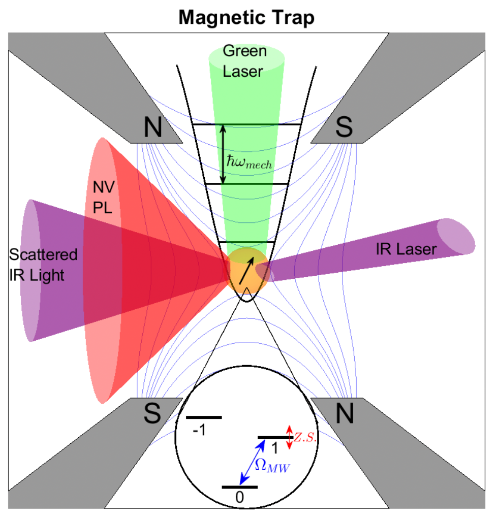
Fig. 1(a) shows the geometry of the magneto-gravitational traps that the proposed experiments will use [10, 25, 11]. Unlike optical or ion traps, which are subject to photon-recoil heating and electric field noise, the magnetic trapping of diamagnetic crystals offers a decoherence-free environment relative to light-matter interactions, potentially enhancing mechanical coherence. The magnetic potential energy for such a particle is given by $U_{B}=-(V/2)(\mu-\mu_{0})\lvert\boldsymbol{H}(x,y,z)\rvert^{2}$, where $\mu_{0}$ is the magnetic permeability of free space, $\mu$ is the magnetic permeability of the particle, and we neglect variations in the field across the particle. Since stable trapping requires $\nabla^{2}U>0$, only diamagnets ($\mu<\mu_{0}$) and superconductors ($\mu=0$) can be stably levitated in static fields. In particular these particles will be repelled by magnetic poles and attracted to field minima. To make traps in all three dimensions, the magnetic flux from two pieces of permanent magnets is focused by four high-magnetization material pole pieces and configured into a quadrupole distribution. For more details on magnetic levitation, see Refs. [10, 11].

To establish the theoretical framework, we begin with a generalized model of a spin-1 system (here, the NV center) coupled to a single motional degree of freedom ($x$) via a linear magnetic gradient. The effective magnetic field along the NV quantization axis is given by $B(x)=B_{0}+\partial B\cdot x$, where $\partial B$ represents the spatial variation of the field. Assuming the mechanical frequency is small relative to the Zeeman splitting, we apply the rotating wave approximation to focus on the longitudinal spin-motion coupling, neglecting rapidly oscillating transverse terms.

Thus, we obtain the toy model Hamiltonian, with $\hbar=1$ [22, 2]:

$$H=DS_{z}^{2}+\gamma_{e}B_{0}S_{z}+2\Omega(t)S_{x}+2gS_{z}(a+a^{\dagger})+\omega a^{\dagger}a$$ (1)

where $D$ is the typical $2\pi\times 2.88$ GHz splitting of the ground state triplet of the NV center, $\Omega(t)$ is the microwave drive used to generate ESR pulses driving the spin, and the harmonic motion of the crystal is given by $\omega$ with creation operator $a^{\dagger}$. We use natural harmonic oscillator units with $g=\gamma_{e}\partial B\ x_{0}/2$ where $x_{0}=\sqrt{\hbar/2m\omega}$ is the harmonic oscillator length, $\omega$ is the harmonic oscillator frequency, and $\gamma_{e}=g^{*}\mu_{B}/\hbar\approx 2\pi\times 27$ GHz/T is the gyromagnetic response of the NV center spin.

For the rest of this paper, we work under the assumption that only two internal states of the NV center are leveraged, for example, 0 and 1, and thus define the pseudospin $\sigma_{z}=\ket{0}\bra{0}-\ket{1}\bra{1}$. This yields a simple two-level model of a spin interacting with a harmonic oscillator:

$$H_{0-1}=\omega_{L}\sigma_{z}/2+\Omega(t)\sigma_{x}+g\sigma_{z}(a+a^{\dagger})+\omega a^{\dagger}a$$ (2)

where $\omega_{L}=\gamma_{e}B_{0}+D$ is the Larmor precession frequency. We will also consider the scenario in which there are multiple (in that case, $N_{s}$) NV centers in the same crystal observing the same gradient as occurs in a more heavily doped crystal.

The rest of this section shall cover how this setup can be used to generate entanglement between the spin and the motion of the diamond and also as a force sensor. We will analyze these settings within the context of various sources of noises, such as thermal noise and backaction.

II.1 Entangling the spins and the mass’s motion

As a matter of principle, this system provides a prototypical system for creating large entangled states, characterized by mechanical superpositions much larger than the harmonic oscillator length $x_{0}$. Specifically, consider the scenario in which one cools the mechanical center-of-mass motion to its ground state, $\ket{\rm vac}$, while the spin is initialized in the $\sigma_{z}=1$ state ($\ket{0}$). Then a $\pi/2$ microwave pulse rotates $\ket{0}$ to $\ket{+}=(\ket{0}+\ket{1})/\sqrt{2}$ [4]. Waiting a time $\tau$, we find in the rotating frame the state

$$\ket{\Psi}= \frac{1}{\sqrt{2}}\left(\ket{0}\ket{-\alpha}+\ket{1}\ket{\alpha}\right)$$ (3)

$$\alpha= -ig\int_{0}^{\tau}e^{-i\omega t}dt=-\frac{g}{\omega}\left[\sin(\omega\tau)+i(\cos(\omega\tau)-1)\right]$$ (4)

where $\ket{\alpha}$ is a coherent state.

For a micrometer-sized diamond particle a typical mass is 3 pg with a mechanical resonance of $\omega=2\pi\times 100$ Hz in a gradient $\partial B\sim 10$ kT/m. This yields $g/\omega\sim 2$. More generally,

$$\frac{g}{\omega}\sim 0.3\left(\frac{dB}{\rm 1\ kT/m}\right)\left(\frac{\rm 1\ pg}{m}\right)^{1/2}\left(\frac{\rm 2\pi\times 100\ Hz}{\omega}\right)^{3/2}$$ (5)

Here, we see that $g/\omega$ is of order unity; a ‘large’ entangled state would be readily accessible if both mechanical and spin coherence times are long enough and if ground state cooling is available.

In principle, this type of entangled state can also be distinguished by use of an entanglement witness – a statistical test of entanglement particularly well suited to combined spin-and-mechanical systems. Following Ref. [21], we construct the following entanglement witness (EW) for this setup:

$$W=1/4\textrm{Var}(\sigma_{x})+\textrm{Var}(\sigma_{y}/2+a_{y}q+b_{y}p)+\textrm{Var}(\sigma_{z}/2+a_{z}q+b_{z}p),$$ (6)

where $\sigma_{\mu}$ is the usual Pauli matrix. In choosing a witness, once has the freedom of choosing $a_{\mu}$ and $b_{\mu}$ to maximize the violation observed for the experimentally-targeted state compared to any separable state. It is assumed that the NV center is in the $\sigma_{x}$ eigenstate $\ket{+}=(1/\sqrt{2})(\ket{0}+\ket{1)}$ at $t=0$. $W$ has the following bound for separable states:

$$W_{b}=\frac{1}{2}+|a_{y}b_{z}-a_{z}b_{y}|$$ (7)

We must also obtain $W_{\textrm{en}}$, where $W_{\textrm{en}}$ is the value taken by Eq. 6 when the variances are evaluated for the expected entangled state, in order to find good choices of $a_{\mu}$ and $b_{\mu}$.

For the single-spin case where the oscillator starts in a thermal state, we can optimize $a_{\mu}$ and $b_{\mu}$, and find that $W_{b}$ and $W_{\rm{en}}$ are given exactly by

$$W_{b}=\frac{1}{2}+\frac{e^{-(2\bar{n}+1)\lambda^{2}[1-\cos(\omega t)]}\cos(\omega_{L}t)\lambda^{2}[1-\cos(\omega t)]}{2\bar{n}+1+2\lambda^{2}[1-\cos(\omega t)]}$$ (8)

$$W_{\rm{en}}=\frac{1}{2}+\frac{1+2\bar{n}}{4(1+2\bar{n}+2\lambda^{2}-2\lambda^{2}\cos(\omega t))}\\ -\frac{e^{-2(1+2\bar{n})\lambda^{2}(1-\cos(\omega t))}}{4}[1+2(1+2\bar{n})\lambda^{2}-2(1+2\bar{n})\lambda^{2}\cos(\omega t)]$$ (9)

For more details on this calculation, see Appendix B.1 and Reference [21].

We now add more detail to this analysis by having the oscillator be in continuous contact with a white noise bath, as can be described by the Hamiltonian

$$\tilde{H}_{0-1}=\omega_{L}\sigma_{z}/2+\Omega(t)\sigma_{x}+(g\sigma_{z}+f_{\textrm{th}}(t))(a+a^{\dagger})+\omega a^{\dagger}a$$ (10)

with (as also discussed in Appendix A)

$$\langle{f_{\rm th}(t)f_{\rm th}(t^{\prime})}\rangle=2\gamma\frac{k_{b}T}{\hbar\omega}\delta(t-t^{\prime}).$$ (11)

(a)

(b)

Figure 3: (a) EW violation when the mass is cooled to its ground state at the start of the experiment and remains in contact with a continuous thermal bath. (b) EW violation when the mass starts in an initial thermal state and remains in contact with a continuous thermal bath. The plots get truncated when the violation becomes negative.

$W_{b}$ and $W_{\rm{en}}$ must now be re-evaluated. Since the expressions are rather complex, we present plots for different scenarios in Figures 3a and 3b. We plot $(W_{b}-W_{\textrm{en}})/W_{b}$, which would be positive if the EW is violated; this quantity also informs us of the number of measurements ($n_{\rm{meas}}$), since $n_{\rm{meas}}\sim[(W_{b}-W_{\textrm{en}})/W_{b}]^{-2}$. It is clear that starting in the ground state is advantageous. We also note that having a larger coupling results in a higher violation, but for a shorter time. In calculating the violation for the case where the oscillator starts in the ground state, we used the coefficients $a_{\mu}$ and $b_{\mu}$ that correspond to the noiseless scenario, while the thermal state coefficients were used when starting in a thermal state.

In reality, applying the EW in Eq. 6 has to overcome the issue of the NV spin having very short coherence times. Indeed, to have coherence times of even 300 $\mu$s, and to also implement back-action evasion, pulse sequences have to be applied. These pulse sequences can result in the decoupling of the spin from the momentum, thus potentially decreasing the effectiveness of this EW, since it relies on correlations between the spin operators and momentum. In Section III.2, we find that Eq. 6 can still be used; however, the exact expressions for $W_{b}$ and $W_{\rm{en}}$ will be modified.

II.2 Force sensing with the entangled state

Next we analyze how the experimental setup can be used as a force sensor by adding an external force to the Hamiltonian,

$$V=-f(a+a^{\dagger}),$$ (12)

where $f=F(t)x_{0}/\hbar$ is in general a time-dependent force, which includes both a signal field and thermal heating effects, as described in Appendix A.

The influence of external forces can be detected by monitoring the NV center spin state, a technique previously demonstrated in Ref. [17]]. To model the limits of our sensing approach, we account for both inhomogeneous broadening, characterized by the Ramsey dephasing time $T_{2}^{*}$, and the dynamical decoherence resulting from temporal magnetic fluctuations, characterized by the Hahn echo time $T_{2}$.

The simplest example of force sensing is given by the Ramsey free evolution sequence, appropriate for when $T_{2}^{*}\omega\gtrsim 1$ . Before going into detail in this calculation, we can build a basic expectation of performance from simple principles.

Projection noise limit: We start by estimating the projection shot noise in the system. Let us first consider the basic principles that determine the effect of the force and the spin, and its observation. The force will move the average center of mass of the diamond by an amount $\sim f/\omega$ when integrated for times $t$ similar to or longer than the mechanical period. This in turn leads to a mean shift in the Larmor frequency of $gf/\omega$. In physical units, $g\frac{f}{\omega}=\frac{\gamma_{e}\partial B}{\omega}Fx_{0}^{2}/\hbar=\gamma_{e}\partial B\ \frac{F}{2m\omega^{2}}$, which is exactly the shift of the Larmor frequency due to the shift of the equilibrium position of the mass from the incident force, as expected.

Thus, as a baseline of expected sensitivity to forces for this type of system, one would hope to be able to achieve at least a sensitivity similar to that of the magnetic sensing of the sensor to this shift in Zeeman energy which is primarily limited by the quantum projection noise and the linewidth ($\sim~1/T_{2}$) , i.e., a force sensitivity of:

$$\eta\sim\frac{\omega}{g\sqrt{T_{2}^{*}}}\ {\rm H.O.\ units}=\frac{2m\omega^{2}}{\partial B\sqrt{T_{2}^{*}}}\ {\rm SI\ units}$$ (13)

where $T_{2}^{*}$ is the inhomogeneous dephasing that we would naively observe with a Ramsey sequence to estimate the resonance frequency.

For a nanogram object with frequency of 1 MHz and a gradient of 10,000 T/m, Eq. (13) yields a sensitivity of $5\times 10^{-11}\text{ N}/\sqrt{\rm Hz}$. If we move instead to a time scale of $T_{2}\ll T_{2}^{*}$, using techniques like spin echo, and reduce the mechanical frequency to a regime with $\omega T_{2}\ll 1$ , we might be able to do much better, down to $10^{-20}$ N/$\sqrt{\rm Hz}$ or lower. Indeed, the levitated trap regime of interest that we now explore has $\omega\sim 2\pi\times 100$ Hz, which provides the opportunity for exquisite force sensitivity, if we are only shot noise limited, i.e., limited by the estimation of the spin being up or down only.

This limit can be improved upon by having more than one NV center contributing to the signal. Using $N_{s}$ contributing spins further improves the sensitivity by $\sqrt{N_{s}}$. For typical micrometer-sized crystals, we expect $N_{s}\lesssim 10^{5}$ for a highly doped crystal, and $\sim 1$ for a lightly doped sample.

Thermal noise considerations: The next practical consideration when building such a force sensor arises from the thermal noise incident on the mechanical system. For a typical Brownian motion bath that describes high Q mechanical system noise when $k_{b}T\gg\hbar\omega$, we expect that the force term includes a thermal noise whose variance grows as $\gamma\frac{k_{b}T}{\hbar\omega}t$ for an integration time $t$. This produces a limit to sensitivity that goes as

$$\eta_{\rm th}\sim\frac{\hbar}{x_{0}}\sqrt{\gamma\frac{k_{b}T}{\hbar\omega}}$$ (14)

in units of N/$\sqrt{\rm Hz}$. At room temperature, this yields $\eta_{\rm th}\approx 2\times 10^{-15}\frac{1}{\sqrt{Q}}(T/300\ {\rm K})$ where $Q=\omega/\gamma$ is the mechanical quality factor. For typical quality factors $Q\gtrsim 10^{5}$, the high magnetic gradient, low frequency, and small mass of levitated systems yield a shot noise that is a larger issue than room temperature thermal noise.

Backaction noise limit: Of course, even if the situation with shot noise is improved, we may eventually be limited by the so-called standard quantum limit. Here, the spin-dependent force on the mass of the diamond leads to backaction, which looks like heating of the center of mass through the measurements. A simple calculation shows that this can be a point of concern, as follows.

First, the spin measurement of $N_{s}$ spins infers the position variable via the frequency shift of the spins; for a spin free precession time of $\tau\lesssim T_{2}^{*}$, we expect an imprecision in position $\Delta x\sim[\gamma_{e}\partial B\tau\sqrt{N_{s}}]^{-1}$ due to the unit spin shot noise. This imprecision leads to an uncertainty in the momentum via the Heisenberg uncertainty relationship $\Delta p\sim\hbar/\Delta x$. If the next measurement occurs a time $\sim t\geq\tau$ later, we can attempt to balance the backaction-induced uncertainty $t\Delta p/m$ with the measurement imprecision $\Delta x$. This is optimized for $t\hbar/m\Delta x=\Delta x$ which yields the SQL and corresponding optimal magnetic gradient:

$$\Delta x_{\rm SQL} =\sqrt{\frac{\hbar t}{m}}\ ,$$ (15)

$$\gamma_{e}\partial B^{*}\sqrt{N_{s}} =\frac{1}{\tau\Delta x_{\rm SQL}}\ .$$ (16)

For a micrometer-sized diamond particle of mass 1.8 pg with 10 ppm NV spins, a target $t=300\ \mu$s corresponding to a 10 Hz resonator, and a $T_{2}\gtrsim 300\ \mu$s, $\partial B\sqrt{N_{s}}>7.5$ kT/m is the gradient necessary to achieve the SQL. This is feasible for small rare earth magnets – thus backaction becomes a point of concern in levitated diamond experiments.

III Backaction evasion and improved entanglement with pulse sequences

Given the above considerations, we recognize that there are substantial practical limits to this sort of approach for sensing. Specifically, the large $g/\omega$ leads to substantial backaction within the short coherence times provided by NV centers, which in turn becomes a limit to the performance of the force sensor. Short coherence times also suggest that the entanglement witness described above will not be realizable in practice, since long coherence times are necessary for an entanglement protocol.

A possible path forward is as follows: using simple echo, or more complex Carr-Purcell, sequences to reduce the backaction, improve the spin coherence, and find a balance between the larger $g/\omega$ and the effects of decoherence and heating. The use of pulses will mean that the EW analysis discussed previously must be adjusted.

In order to understand why pulse sequences are required, we shall now consider the specifics of measuring the spin precession due to the incoming force. As different pulse sequences are considered, in the interaction picture we will take the coupling $g$ to be time dependent, flipping sign every time a $\pi$ pulse is applied to the spin. Here, we do the calculation for the free evolution period, with $g(t)$ taking into account whether a pulse has been applied or not. We see in the Heisenberg picture that we get Larmor precession for a time $\tau$ during Ramsey interferometry that yields a rotation angle around the $z$ axis of

$$\phi_{\rm R} =-\omega_{L}\tau-\int_{0}^{\tau}g(t){\rm Re}[a(t)]dt$$ (17)

$$a(t) =a_{0}e^{-i\omega t}-i\int_{0}^{t}e^{-i\omega(t-t^{\prime})}[g(t^{\prime})S_{z}-f(t^{\prime})]dt^{\prime}$$ (18)

where we recognize that for the free evolution period $S_{z}$ is a constant of motion.

From these equations, we see that the rotation of the spin (its phase) from the mass has two terms. One is a contribution from the spin itself, which leads to spin squeezing, whose amplitude for constant $g$ (Ramsey) is given by $\frac{2g^{2}}{\omega^{2}}(\cos(\omega\tau)-1)$. Thus choosing $\tau\omega=2\pi n$ for $n\in\mathbb{Z}$ eliminates this effect, though later we will look at using the squeezing as a resource. The second term is best understood by taking the Fourier transform of the incoming force $f(t)=\int_{-\infty}^{\infty}f(\nu)e^{-i\nu t}\frac{d\nu}{\sqrt{2\pi}}$. This gives for constant $g$:

$$\phi_{R,f}=\int f(\nu)\frac{2(\nu[\cos(\omega\tau)-1]-\omega[\cos(\nu\tau)-1])}{\nu\omega(\nu-\omega)}\frac{d\nu}{\sqrt{2\pi}}\\ =\int\chi(\nu)f(\nu)d\nu$$ (19)

It is convenient to rewrite the spin phase using a response function $\chi(\nu)$, defined by the above. When $\tau=2\pi/\omega$, $\chi(\nu)$ is maximal for $\nu=\omega/2$, with value $-16g/\omega^{2}$. Intuitively, the spin accumulates a phase from the force that goes as $g$ times the displacement due to the force integrated over the period $\sim f/\omega\times\tau\sim f/\omega^{2}$.

Curiously, we note that there is nominally no backaction on the mass from the measurement of this force. To see this explicitly, we can look at the spin-dependent displacement $\frac{1}{2}\partial_{S_{z}}a(t)$ which is

$$\sqrt{\Delta n}=\frac{1}{2}\left|\int_{0}^{\tau}e^{-i\omega(\tau-t^{\prime})}g(t^{\prime})dt^{\prime}\right|$$ (20)

where we look at the induced displacement from the spin in terms of how many phonons are excited, $\Delta n$. For Ramsey interferometry, we find $\Delta n=\frac{4g^{2}\sin^{2}(\omega\tau/2)}{\omega^{2}}$. Specifically, the spin-dependent force term integrates to zero for $\omega\tau=2\pi n$. However, in practice, this is difficult to achieve while maintaining a good ‘duty cycle’; we would like $T_{2}^{*}\omega\sim 1$ to reduce backaction, but levitated trap frequencies are generally quite slow, e.g., tens of Hz compared to $T_{2}^{*}\sim 1-10\ \mu$s. Thus, to be in the regime of reduced backaction, we want to both consider using spin echo techniques to improve spin coherence and look at measuring forces with bandwidths greater than $\omega$, which we call broadband sensing.

The large $g/\omega$ afforded by our setup is favorable for the generation of entanglement. However, our entanglement detection protocol consists of the EW given in Eq. 6, which relies on measuring correlations between spin and momentum. Employing pulse sequences can destroy such correlations, as can be seen in Figure 2. Therefore, we must confirm that the EW can still be used.

III.1 Broadband sensing with pulse sequences

It is natural to consider a Hahn echo [8] or Carr-Purcell-type sequence [5] to improve the spin coherence towards $T_{2}$. This comes at the cost of a reduced response to the incoming force. However, as we will show, the total impact is minimal for broadband or high frequency signals.

We can now ask what happens to (1) the spin and (2) the harmonic motion when we do a Ramsey, spin-echo, or Carr-Purcell sequence on the electron spin during evolution. Of particular interest will be a variant of the Carr-Purcell sequence in which we do two $\pi$ pulses, as follows: free evolve for $t_{1}$, then $\pi$, then free evolve for $t_{1}+t_{2}$, then $\pi$, then a final evolution for $t_{2}$. The total time $\tau\approx 2t_{1}+2t_{2}$, and we see that DC spin noise leading to $T_{2}^{*}$ is completely removed. At the same time, we do get a small amount of backaction. For $t_{1}\omega,t_{2}\omega\ll 1$, we find that setting $t_{1}=t_{2}=\tau/4$ leaves behind a total impulse of

$$\Delta n_{\rm CP}=\frac{g^{2}}{\omega^{2}}2^{6}\sin^{4}(\omega\tau/8)\sin^{2}(\omega\tau/4)\sim 2^{-10}\omega^{4}g^{2}\tau^{6}$$ (21)

and that this is optimal for $\omega\tau\ll 1$.

At the same time, we accumulate a force signal from DC to $\sim 2\pi/\tau$ that is approximated by

$$\phi_{\rm CP}\approx\frac{g\omega\tau^{3}}{2^{5}}\int_{-\infty}^{\infty}f(\nu)e^{-i\nu\tau/2}e^{-(9\omega^{2}+\nu^{2})\tau^{2}/2^{6}}\frac{d\nu}{\sqrt{2\pi}}$$ (22)

for $\nu\tau\lesssim 2\pi$ and $\omega\tau\ll 1$. We plot this approximation and the actual spectral response function in Fig. 7 of Appendix A).

The relative performance of the three sensing modalities—Ramsey, Hahn echo, and Carr-Purcell—is evaluated for a fixed measurement bandwidth $\sim 2\pi/\tau$. In the low-frequency regime where $\omega\tau\ll 1$, the sensitivities of these sequences are compared in Table 1.

Table 1: The spin accumulation $\phi$ normalized by the coupling $g$ and unit incoming force $f$, compared against the heating due to spin projection noise in units of harmonic oscillator quanta divided by the coupling $g^{2}$. All of these are calculated for signals with $|\nu|<2\pi/\tau$, and have total sequence times of $\tau$.

Seq.	$\phi/(gf)$	$\Delta n/g^{2}$	Force SQL$/\xi^{1/4}$	SQL coupling $g^{*}$ ($\xi=1/4$)
Ramsey	$\frac{\omega\tau^{3}}{6}$	$\tau^{2}$	$\frac{6\tau}{\omega\tau^{3}}=\frac{6}{\omega\tau^{2}}$	$\frac{1}{\tau\sqrt{N}}$
Hahn echo	$\frac{\omega\tau^{3}}{8}$	$\frac{\omega^{2}\tau^{4}}{16}$	$\frac{8\omega\tau^{2}}{4\omega\tau^{3}}=\frac{2}{\tau}$	$\frac{4}{\omega\tau^{2}\sqrt{N}}$
Carr-Purcell	$\frac{\omega\tau^{3}}{32}$	$\frac{\omega^{4}\tau^{6}}{1024}$	$\frac{32\omega^{2}\tau^{3}}{32\omega\tau^{2}}=\omega$	$\frac{32}{\omega^{2}\tau^{3}\sqrt{N}}$

(a)

(b)

(c)

Figure 4: Plots of sensitivity vs various parameters. Different colors indicate the various types of pulse sequences, while solid lines are for $\bar{n}/Q=1$ and dashed lines are for $\bar{n}/Q=10^{4}$ (as also shown in the plot legend). (a) 1 $\mu$m radius diamond, 100 Hz trap, $Q=10^{6}$, cooling time $t_{c}$ = 100 $\mu$s, cooling rate $\gamma_{c}=$ 1 kHz, and an expected signal frequency of 2 kHz. (b) Optimal g, fixed input of 2 kHz (c) Optimal g, fixed time of 100 $\mu$s.

Of specific interest is the notional force SQL for each approach to sensing. This arises when considering a sequence of measurements, where the occupation of the harmonic oscillator mode with phonons leaves behind a signal which is comparable to the heating, e.g., a phase noise in the signal that goes as $\sqrt{\Delta n}$. If there is a short cooling period $t_{c}$ with cooling rate $\gamma_{c}$, this gives a steady-state occupation of the harmonic oscillator purely from backaction of

$$n^{*}=\xi\Delta n$$ (23)

where $\xi\equiv\frac{e^{-\gamma_{c}t_{c}}}{1-e^{-\gamma_{c}t_{c}}}$ gives the effect of cooling over many cycles. When we include this term in the noise-to-signal calculation, we have for the noise squared $1/4+(\Delta n)n^{*}$, where the first term comes from spin projection noise and the second term from the backaction-induced heating which includes a short cooling period. The noise-to-signal ratio is then

$$\frac{1/4+(\Delta n)^{2}\xi}{\phi^{2}}$$ (24)

As $\phi\sim g$ and $\Delta n\sim g^{2}$, we find a SQL-like behavior for force sensing at an optimal $g$ such that $1/4=(\Delta n)^{2}\xi$, which gives as the force SQL $\sim\sqrt{\sqrt{\xi}\Delta n}/|\phi/f|$ which is, as expected, $g$-independent. Comparing the different protocols, we see that the Carr-Purcell sequence well outperforms (has the lowest force SQL) compared to the other sequences for $\omega\tau\ll 1$.

To evaluate the system’s performance, we conduct a numerical study using realistic experimental parameters: a 1 $\mu$m diamond crystal situated in a 100 Hz magnetic trap. Our model incorporates several practical constraints, including a finite experimental duty cycle due to 100 $\mu$s of reset and cooling between measurements, and a finite cooling rate $\kappa$ of 1 kHz. We also consider two different $\bar{n}/Q$ values: $1$ and $10^{4}$. In the subsequent analysis, we work near a bandwidth comparable to $1/T_{2}\sim 10$ kHz, since a typical signal of interest is as such.

The influence of external forces is detected by monitoring the NV center spin state, a technique previously established in the literature [17]. We analyze the sensitivity of this detection channel as follows.

The optimization process begins by determining the ideal effective coupling strength, $g\sqrt{N_{s}}$, as illustrated in Fig. 4a. As the coupling gets larger, the more complex sequences start to outperform the simpler sequences due to the reduced dependence on the thermal background. This leads to a higher $g$ before backaction effects.

Upon determining the optimal effective coupling, we investigate the impact of the free evolution period $\tau$ on measurement precision. As shown in Fig. 4b, $\tau\nu\sim 1$ appears optimal.

Finally, by fixing $\tau$ and sweeping the signal frequency $\nu$, we characterize the spectral response of each sensing modality (Fig. 4c). Our analysis reveals distinct operational regimes for each sequence. For both Ramsey and echo sequences, we have a flat response at low frequencies – they operate as broadband force sensors and are sensitive to DC forces. In contrast, the Carr-Purcell sequence has less sensitivity at lower frequencies, consistent with the usual behavior of a back-action evading impulse detector. Thus for impulse metrology it is likely the optimal approach when compared to the other options.

III.2 Entanglement witness with pulse sequences

Next we must understand how the pulse sequences affect the EW in Equation 6. Motivated by Fig. 2, we expect there to be some equivalency between the Ramsey sequence state at $\tau=\pi/\omega$ with the Echo sequence at $\tau\ll\pi/\omega$.

If we consider the basic Hamiltonian without pulses to be

$$H_{0-1}=g\sigma_{z}(a+a^{\dagger})+\omega a^{\dagger}a,$$ (25)

where we have dropped the Larmor precession and pulse terms of Eq. 2, we find that the unitaries with and without pulses to be given by

$$U_{\rm{pulseless}}=D^{\dagger}(g\sigma_{z}/\omega)e^{-i\omega a^{\dagger}a\tau}D(g\sigma_{z}/\omega)$$ (26)

$$U_{\rm{pulse}}=D(g\sigma_{z}/\omega)e^{-i\omega a^{\dagger}a\tau/2}D(-2g\sigma_{z}/\omega)e^{-i\omega a^{\dagger}a\tau/2}D(g\sigma_{z}/\omega)$$ (27)

The derivation for these unitaries is provided in Appendix B.3. One can see that the spin-motion coupling term in the Hamiltonian appears in the displacement operators; thus, we expect that the coupling results in some displacement of the initial coherent state.

We can now apply these unitaries to the initial state $\ket{\alpha}(\ket{0}+\ket{1})/\sqrt{2}$, where $\ket{\alpha}$ is an arbitrary coherent state. The general expressions for the resulting states are given in Eqs 77 and 78. At $\tau=\pi/\omega$ for $U_{\rm{pulseless}}$ and $\tau\ll\pi/\omega$ for $U_{\rm{pulse}}$, we get:

$$\ket{\psi}_{\rm{pulseless}}=\frac{1}{\sqrt{2}}\ket{-\alpha-\frac{2g}{\omega}}\ket{0}+\frac{1}{\sqrt{2}}\ket{-\alpha+\frac{2g}{\omega}}\ket{1}$$ (28)

$$\ket{\psi}_{\rm{pulse}}=\frac{1}{\sqrt{2}}\ket{\alpha\mathcal{H}(\omega,\tau)-\frac{1}{4}\omega g\tau^{2}}\ket{0}\\ +\frac{1}{\sqrt{2}}\ket{\alpha\mathcal{H}(\omega,\tau)+\frac{1}{4}\omega g\tau^{2}}\ket{1}$$ (29)

where $\mathcal{H}(\omega,\tau)$ is simply the expansion of $e^{-i\omega t}$ in $\omega\tau$; that is, $\mathcal{H}(\omega,\tau)=\left(1-\frac{1}{2}\omega^{2}\tau^{2}-i\omega\tau\right)$.

Note that the key difference between Equations 28 and 29 is the change $\pm 2g/\omega\rightarrow\pm(1/4)\omega g\tau^{2}$.

The EW calculations in Section II.1 were for the pulse-less case; at t = $\pi/\omega$ (and $\omega_{L}=0$), the relevant quantities evaluate to:

$$a_{y} =0$$ (30)

$$b_{y} =\sqrt{\frac{2}{m\omega}}\lambda e^{-2(2\bar{n}+1)\lambda^{2}}$$ (31)

$$a_{z} =\sqrt{2m\omega}\frac{\lambda}{(1+2\bar{n}+4\lambda^{2})}$$ (32)

$$b_{z} =0$$ (33)

and

$$W_{\rm{b}} =\frac{1}{2}+\frac{2e^{-2(1+2\bar{n})\lambda^{2}}\lambda^{2}}{1+2\bar{n}+4\lambda^{2}}$$ (34)

$$W_{\rm{en}} =\frac{1}{2}+\frac{1+2\bar{n}}{4(1+2\bar{n}+4\lambda^{2})}-\frac{e^{-4(1+2\bar{n})\lambda^{2}}}{4}[1+4(1+2\bar{n})\lambda^{2}]$$ (35)

Since for $U_{\rm{pulseless}}$, we had $\lambda=2g/\omega$, the difference between Eqs. 28 and 29 would suggest that for $U_{\rm{pulse}}$, we can still use the results in Eqs. 30-35, but with $\lambda$ now replaced with $(1/4)\omega g\tau^{2}$. We plot the results in Figure 6. Figure 6a shows the violation against $\bar{n}$ at $\tau=0.1\times\pi/\omega$ for different values of $g$. Figure 6b plots the time at which the (log plot of the) violation asymptotes (i.e. violation ceases to occur) against $\bar{n}$. As expected, we see that increasing $\bar{n}$ reduces the duration for which violation exists; notably, the higher value of $g/\omega$, the smaller the value of $\tau_{\rm{asymp}}\times\omega/\pi$ for a given value of $\bar{n}$. Next, in Fig. 6c, we plot $\bar{n}$ vs $\tau^{*}\times\omega/\pi$, which is the time at which violation $(W_{b}-W_{\rm{en}})/W_{b}$ reaches $10^{-3}$ (that is, the time at which the required number of measurements to detect this violation reaches $10^{6}$). We see that the maximum $\bar{n}$ is independent of $g/\omega$; indeed, it seems as though the plots for the different values of $g/\omega$ are the same – they appear to be simply shifted over time.

Figure 5: A visual representation of the resulting states that occur with pulse sequences, with and without a thermal bath. $\gamma$ refers to the parameters of an arbitrary coherent state $\ket{\gamma}$. Diagram is not to scale. (a) Depiction of Eq. 28, where $\ket{-\alpha}$ (in grey) is translated by $\pm 2g/\omega$ (to pink). (b) Depiction of Eq. 29, where $\ket{\alpha}$ (in grey) is translated by $\pm(1/4)\omega g\tau^{2}$ (to purple).

(a)

(b)

(c)

Figure 6: (a) We plot the violation against $\bar{n}$ for different values of $g$. Here, $\lambda=(1/4)\omega g\tau^{2}$ and we have also set $\omega=2\pi\times 100$ Hz and $\tau=0.1\times\pi/\omega$. Note that the plots truncate (i.e. violation ceases to exist) at $\bar{n}\sim O(1)$. Additionally, the higher the value of $g/\omega$, the lower the value of $\bar{n}$ at which the violation stops. The data in these figures have been extracted from plots similar to that of Figure 6a and are thus for the case where the oscillator starts in a thermal state (but with no continuous thermal bath) (b) For different $g/\omega$, we extract $\tau\times\omega/\pi$ and $\bar{n}$ at the point where $\log_{10}[(W_{b}-W_{\rm{en}})/W_{b}]$ asymptotes, i.e. violation of the EW ceases to exist. Thus, this plot tells us of the maximum time period for which violation exists as $\bar{n}$ increases. As expected, the higher the value of $\bar{n}$, the shorter the duration for which violation exists. (c) For different $g/\omega$, we extract $\tau\times\omega/\pi$ and $\bar{n}$ at the point where $\log_{10}[(W_{b}-W_{\rm{en}})/W_{b}]$ has a value of $-3$; this $\tau$ is represented as $\tau^{*}$. Thus, this figure gives us the maximum $\bar{n}$ allowed for a violation $(W_{b}-W_{\rm{en}})/W_{b}$ of at least $10^{-3}$, which means the protocol would require at most $10^{6}$ measurements. Notably, the maxima of the plots for different values of $g/\omega$ are the same, indicating that the maximum allowed $\bar{n}$ is independent of $g/\omega$.

IV Squeezing

Table 2: Squeezing for each pulse sequence relative to the spin-motion coupling $g$, taking $\xi=1/4$.

Seq.	$\zeta/g^{2}$	Squeezing at SQL
Ramsey	$\frac{\omega\tau^{3}}{6}$	$\frac{\omega\tau}{6N_{s}}$
Hahn echo	$\frac{\omega\tau-4\sin(\omega\tau/2)+\sin(\omega\tau)}{\omega^{2}}\sim\frac{\omega\tau^{3}}{12}$	$\frac{4}{3\omega\tau N_{s}}$
Carr-Purcell	$\frac{\omega\tau-4\sin(\omega\tau/4)-4\sin(\omega\tau/2)+4\sin(3\omega\tau/4)-\sin(\omega\tau)}{\omega^{2}}\sim\frac{\omega\tau^{3}}{48}$	$\frac{64}{3\omega^{3}\tau^{3}N_{s}}$

The performance of complex pulse sequences only matters if we have sufficiently strong coupling to achieve the SQL, and if thermal noise and other sources are sufficiently weak. As shown above, this may not be relevant for the case of single spins. For example, a micrometer-sized diamond with 10 ppm NV centers has more than $N_{s}\sim 10^{5}$ NVs within it. Many of the results above immediately scale to the case of $N_{s}$ spins. Generically we expect for $n^{*}$ to increase by a factor of $N_{s}$ due to the independent sum of each spin’s backaction, while $\Delta n$ is the same for a single spin’s phase evolution. At the same time, the spin projection noise is reduced by $\sqrt{N_{s}}$. Thus the $N_{S}$-dependent noise to signal ratio is

$$NSR_{\rm N}\sim\frac{1/4N_{s}+N_{s}(\Delta n)^{2}\xi}{\phi^{2}}$$ (36)

We see that this acts effectively as an increase of $g\rightarrow g\sqrt{N_{s}}$, as would be naively expected. The SQL is thus

$$g^{*}\sqrt{N_{s}}=\frac{1}{\sqrt{2(\Delta n/g^{2})\sqrt{\xi}}}$$ (37)

For the case of Carr-Purcell, this yields $g^{*}\sqrt{N_{s}}\sim 2^{5}/\omega^{2}\tau^{3}$.

However, when using $N_{s}$ spins, we also have a new term that emerges: the spin projection $J_{z}\equiv\sum_{j}S_{z}^{j}$ produces a force on the mechanical system, that in turn causes a rotation around the $z$ axis of the spins that is proportional to the spin projection. This is a type of squeezing, represented by $\exp(-i\zeta J_{z}^{2})$ as a unitary operation. As shown in Appendix A, this $\zeta$ parameter is given by

$$\zeta=\int_{0}^{\tau}\int_{0}^{t}\sin(\omega(t-t^{\prime}))g(t)g(t^{\prime})dt^{\prime}dt$$ (38)

where $g(t)$ is the coupling that changes sign due to the various pulses used in a given sequence.

For our three sequences of choice, we have the squeezing going similarly, as shown in Table 2, going as $\zeta\sim g^{2}\omega\tau^{3}$. We can now compare this to the force SQL, which gives a value of $g^{*}$ that is nominally ideal. We see that for $\omega\tau\ll 1$, the squeezing at SQL from the higher order pulse sequences is far larger than for the smaller sequences. Even for modest $\omega\tau$, the large numerators and prefactors indicate that squeezing will in general be accessible and must be accounted for when doing sensing with many spins.

Now we can ask: can we use squeezing during the sequence to improve the force sensing capabilities of the system? We find the answer to be ‘yes’ in practice, if we make a small rotation of the final observable – rather than measuring, e.g., $J_{y}$, we instead do an additional rotation about the $x$ axis of the spin by an angle

$$\theta=-\tan^{-1}\left(\frac{4}{N_{s}\zeta}+\frac{N_{s}\zeta}{2}\right)$$ (39)

This improves the signal to noise by reducing the spin shot noise as

$$\frac{1}{\sqrt{N_{s}}}\rightarrow\frac{1}{\sqrt{N_{s}}\sqrt{1+(N_{s}\zeta/4)^{2}}}$$ (40)

for $\zeta N_{s}\ll\sqrt{N_{s}}$. The limit on large $\zeta N_{s}$ reflects a breakdown of the bosonic approximation to the spin variables $J_{y}$ and $J_{z}$. This also confirms that this approach is unlikely to approach the Heisenberg limit, though it is a practical improvement.

Thus our system combines both backaction evasion and sub-Poissonian statistics, which occurs naturally in the high Q limit so long as the phonon heating rate is sufficiently low, as may be realized in levitated systems. We note that these benefits are also limited by, e.g., $T_{2}$ for Carr-Purcell sequences and will depend sensitively on many specific parameters of the system.

V Outlook

In this paper, we proposed a sensing system composed of an NV center spin coupled to the motion of its levitated host diamond, where the interaction between the spin and the diamond results from the gradient of the magnetic trap. We find that shot noise limits force sensitivity more than room temperature thermal noise and that backaction is significant enough to be addressed. Backaction evasion with a Carr-Purcell-type sequence can significantly enhance the sensitivity of this sensor to forces; in particular, we find that we can obtain sensitivities $<10^{-23}$ at frequencies of $10^{4}$ Hz. We also investigate the generation of entanglement between the spin and the motion of the diamond using an entanglement witness (EW); once appropriate modifications are made, the same witness that is used for the case without pulses can be used when pulse sequences are applied. For the EW, as expected, starting in a thermal state results in a shorter duration of violation, especially as the thermal occupancy ($\bar{n}$) is increased, as does the introduction of a thermal bath. If entanglement generation is a priority, it is advantageous to start with a diamond that has been cooled to the ground state.

A setup such as this has practical applications in force sensing and testing the quantum nature of forces. Indeed, our experimental-theoretical collaboration is attempting to practically implement a force sensor as described here. We are also interested in seeing if our apparatus can result in spin-motion entanglement, although we may have to use an alternative method to verify the generation of entanglement, given the requirement of measuring both the position and momentum of the diamond for the current witness.

VI Acknowledgments

This work was supported by the John Templeton Foundation (Grant No. 63121). G.P. also acknowledges support from the Heising-Simons Foundation (Grant No. 2023-4467), while G.D., J.B., and D.P. were further supported by the Sloan Foundation (Grant No. G-2023-21131).

Appendix A Pulsed evolution picture

Consider the evolution under a sequence of $n$ microwave pulses $P_{i}$ applied to the spins. We write the total evolution as a series of unitary evolutions interleaved with pulses, as

$$U(t_{f},t_{0})=U(t_{f},t_{n})P_{n}U(t_{n},t_{n-1})P_{n-1}\ldots P_{1}U(t_{1},t_{0})$$ (41)

From this we can define an interaction picture between $P_{i}$ and $P_{i+1}$ as

$$U_{I}(t_{i+1},t_{i})=(\prod_{j\leq i}P_{j})^{\dagger}U(t_{i+1},t_{i})(\prod_{j\leq i}P_{j})$$

In the case of only $\pi$ pulses, this corresponds to changes to sign of the pseudo spin $\sigma_{z}=\ket{1}{1}-\ket{0}\bra{0}$. Thus we can write the Hamiltonian $H_{I}(t)$ in this interaction picture:

$$H_{I}=[-f(t)+g(t)\sigma_{z}](ae^{-i\omega t}+a^{\dagger}e^{i\omega t})$$ (42)

where the pulses determine the sign of $g$ over time.

Figure 7: Numerical evaluation of the approximation (Eqn. 22 appropriate for the response function $\chi(\nu)$ of the Carr-Purcell sequence (of length $T/4$) for $T=0.2~\pi/\omega$ (purple) and $T=0.05~\pi/\omega$ (pink). The plot is made unitless by comparing $\nu$ to $\omega$ and $\chi$ to $\omega^{-1}$. The approximation is appropriate for frequencies comparable to or below the bandpass $2\pi/T$.

Within this formalism, we note that we can find the exact form of $U$ by using the Magnus expansion, as $[H_{i}(t),[H_{i}(t^{\prime}),H_{i}(t^{\prime\prime})]]=0$. That is,

$$U(t_{f},t_{0}) =\exp[-i(\Phi_{1}+\Phi_{2})]$$ (43)

$$\Phi_{1} =\int_{t_{0}}^{t_{f}}H_{I}(t^{\prime})dt^{\prime}$$ (44)

$$\Phi_{2} =\frac{1}{2i}\int_{t_{o}}^{t_{f}}\int_{t_{o}}^{t^{\prime}}[H_{I}(t^{\prime}),H_{I}(t^{\prime\prime})]dt^{\prime\prime}dt^{\prime}$$ (45)

Exploring these two terms, we have

$$\Phi_{1}=\int_{t_{0}}^{t_{f}}(-f(t^{\prime})+g(t^{\prime})\sigma_{z})e^{-i\omega t^{\prime}}dt^{\prime}a+{\rm H.c.}$$ (46)

and thus this term contributes an overall (spin-dependent) displacement to the harmonic oscillator from the spin and from the external force.

We now turn to the second term, which combines the effects of the force and of the spin-dependent interaction – this yields a rotation of the spins that depends upon the force, and thus is our force signal of interest. Specifically,

$$\Phi_{2}=\int_{t_{o}}^{t_{f}}\int_{t_{o}}^{t^{\prime}}\sin(\omega(t^{\prime}-t^{\prime\prime}))(-f(t^{\prime})+g(t^{\prime})\sigma_{z})\\ \times(-f(t^{\prime\prime})+g(t^{\prime\prime})\sigma_{z})dt^{\prime\prime}dt^{\prime}\ .$$ (47)

If we look at an ensemble of spins with $J_{z}=1/2\sum_{i}\sigma_{z}^{i}$, then we see that $\Phi_{2}$ has two main contributions: phase evolution from the $fg$ cross term, and squeezing from the $g(t^{\prime})g(t^{\prime\prime})$ term. The term proportional to $f(t^{\prime})f(t^{\prime\prime})$ is a global phase and not observable.

$$\Phi_{2}=-2g_{i}J_{z}\int_{t_{i}}^{t_{i+1}}\int_{t_{i}}^{t^{\prime}}\sin(\omega(t^{\prime}-t^{\prime\prime}))(f(t^{\prime})+f(t^{\prime\prime}))dt^{\prime\prime}dt^{\prime}\\ +4g_{i}^{2}J_{z}^{2}\frac{\tau_{i}\omega-\sin(\tau_{i}\omega)}{\omega^{2}}$$ (48)

where $\tau_{i}=t_{i+1}-t_{i}$. This second term has a phase evolution under $J_{z}$ that is determined by the external force, and a squeezing term $\propto J_{z}^{2}$.

We remark that the approach we use in this paper – which neglects explicit mechanical damping – is appropriate when we are in the high $Q$ and high temperature regime $k_{b}T\gg\hbar\omega$ for the mechanical system. In this limit, the dominant effect of the mechanical environment is that of classical Brownian motion noise. That is,

$$f(t)\rightarrow f(t)+f_{\rm th}(t)$$ (49)

with

$$\langle{f_{\rm th}(t)f_{\rm th}(t^{\prime})}\rangle=2\gamma\frac{k_{b}T}{\hbar\omega}\delta(t-t^{\prime})$$ (50)

In SI units, this is the usual $4m\gamma k_{b}T\delta(t-t^{\prime})$.

This high temperature approximation captures the dominant errors in measurement.

Appendix B Entanglement witness elaboration

Here we provide more details on the EW calculation. In order to determine $W_{\textrm{en}}$, we need to evaluate terms such as $\bra{\psi_{\textrm{in}}}\sigma_{x}(t)^{2}\ket{\psi_{\textrm{in}}}$, $\bra{\psi_{\textrm{in}}}\sigma_{y}(t)q(t)\ket{\psi_{\textrm{in}}}$, $\bra{\psi_{\textrm{in}}}\sigma_{y}(t)p(t)\ket{\psi_{\textrm{in}}}$ etc, with $\ket{\psi_{\textrm{in}}}=\ket{\psi_{s,\textrm{in}}}\otimes\ket{\psi_{\textrm{osc},\textrm{in}}}$, where $\ket{\psi_{s,\textrm{in}}}$ is the initial state of the spin and $\ket{\psi_{\textrm{osc},\textrm{in}}}$ is the initial state of the oscillator (diamond). For this, it is convenient to consider the Heisenberg evolution of operators under the appropriate Hamiltonian.

B.1 Noiseless EW

For the EW evaluation, we adopt the calculations in Ref. [21], after incorporating suitable modifications. Defining $\tilde{S}_{z}=\sigma_{z}/2$, for the noiseless case we can start from

$$\phi_{\rm ent} =\omega_{L}t+\int_{0}^{t}2g[a(t^{\prime})+a^{\dagger}(t^{\prime})]dt^{\prime}$$ (51)

$$a(t) =a_{0}e^{-i\omega t}-i\int_{0}^{t}e^{-i\omega(t-t^{\prime})}2g\tilde{S}_{z}~dt^{\prime},$$ (52)

and for the spin operators,

$$\tilde{S}_{x}(t)=\tilde{S}_{x}\cos(\phi_{\textrm{ent}})-\tilde{S}_{y}\sin(\phi_{\textrm{ent}})$$ (53)

$$\tilde{S}_{y}(t)=\tilde{S}_{y}\cos(\phi_{\textrm{ent}})+\tilde{S}_{x}\sin(\phi_{\textrm{ent}})$$ (54)

with

$$\phi_{\textrm{ent}}=\omega_{L}t+\sqrt{\frac{2}{m\omega}}~\lambda p[1-\cos(\omega t)]+\sqrt{2m\omega}~\lambda q\sin(\omega t),$$ (55)

where $\lambda=2g/\omega$, and for the oscillator operators

$$q(t)=q\cos[\omega t]+\frac{p}{m\omega}\sin[\omega t]+\sqrt{\frac{2}{m\omega}}\lambda\tilde{S}_{z}[\cos(\omega t)-1]$$ (56)

$$p(t)=p\cos(\omega t)-m\omega q\sin(\omega t)-\sqrt{2m\omega}\lambda\tilde{S}_{z}\sin(\omega t)$$ (57)

Using Eqs. 53-57 and expanding, we are left to evaluate terms such as $\bra{\psi_{\textrm{in}}}O_{s}O_{\textrm{osc}}\ket{\psi_{\textrm{in}}}$, which, as a result of $\ket{\psi_{\textrm{in}}}$ being separable, ultimately requires us to determine $\bra{\psi_{\textrm{s,in}}}O_{s}\ket{\psi_{\textrm{s,in}}}$ and $\bra{\psi_{\textrm{osc,in}}}O_{\textrm{osc}}\ket{\psi_{\textrm{osc,in}}}$.

Once $W_{\textrm{en}}$ is in hand, we will consider the quantity

$$W_{\textrm{ratio}}=\frac{W_{b}-W_{\textrm{en}}}{W_{b}}$$ (58)

since the number of measurements required to determine this violation is $\sim W_{\textrm{ratio}}^{-2}$. We choose the coefficients $a_{\mu}$ and $b_{\mu}$ as explained in Ref. [21]; we choose by solving for $a_{\mu}$ and $b_{\mu}$ for $\partial_{a_{\mu}}W_{\textrm{en}}=0$ and $\partial_{b_{\mu}}W_{\textrm{en}}=0$.

B.2 Thermal bath

We must recalculate $W_{\rm{en}}$ and $W_{b}$ for the case of the thermal bath. We follow the same calculation as in Ref. [21] after some simple modifications to numerical factors. With

$$\phi_{\rm ent,th} =\omega_{L}t+\int_{0}^{t}2g[a(t^{\prime})+a^{\dagger}(t^{\prime})]~dt^{\prime}$$ (59)

$$a(t) =a_{0}e^{-i\omega t}-i\int_{0}^{t}e^{-i\omega(t-t^{\prime})}(2g\tilde{S}_{z}+f_{\textrm{th}}(t^{\prime}))~dt^{\prime},$$ (60)

the noise contribution to the position, momentum, and rotation angle will then be:

$$\mathcal{Q} =-2q_{\textrm{zpf}}\int_{0}^{t}f_{\textrm{th}}(t^{\prime})\sin[\omega(t-t^{\prime})]~dt^{\prime}$$ (61)

$$\mathcal{P} =-2p_{\textrm{zpf}}\int_{0}^{t}f_{\textrm{th}}(t^{\prime})\cos[\omega(t-t^{\prime})]~dt^{\prime}$$ (62)

$$\Phi=2g\int_{0}^{t}\frac{\mathcal{Q}(t^{\prime})}{q_{\textrm{zpf}}}~dt^{\prime}\\ =-4g\int_{0}^{t^{\prime}}\int_{0}^{t}f_{\textrm{th}}(t^{\prime})\sin(\omega(t^{\prime}-t^{\prime\prime}))~dt^{\prime\prime}dt^{\prime}$$ (63)

With these, and using,

$$\langle{f_{\rm th}(t)f_{\rm th}(t^{\prime})}\rangle=2\gamma\frac{k_{b}T}{\hbar\omega}\delta(t-t^{\prime}),$$ (64)

we find that the total noise contribution is:

$$\Delta\langle{\textrm{Var}(\tilde{S}_{x})}\rangle =\frac{1}{2}\lambda^{2}\frac{\bar{n}}{Q}[6\omega t-8\sin(\omega t)+\sin(2\omega t)]$$ (65)

$$\Delta\langle q^{2}\rangle =2q_{\textrm{zpf}}^{2}\frac{\bar{n}}{Q}[2\omega t-\sin(2\omega t)]$$ (66)

$$\Delta\langle p^{2}\rangle =2p_{\textrm{zpf}}^{2}\frac{\bar{n}}{Q}[2\omega t+\sin(2\omega t)]$$ (67)

$$\Delta\langle qp+pq\rangle =4\frac{\bar{n}}{Q}\sin^{2}(\omega t)$$ (68)

$$\Delta\langle\tilde{S}_{y}q+q\tilde{S}_{y}\rangle =-16\lambda\frac{\bar{n}}{Q}q_{\textrm{zpf}}\sin^{4}(\omega t/2)$$ (69)

$$\Delta\langle\tilde{S}_{y}p+p\tilde{S}_{y}\rangle =8\lambda\frac{\bar{n}}{Q}p_{\textrm{zpf}}\left[\frac{\omega t}{2}-\sin(\omega t)+\frac{\sin(2\omega t)}{4}\right]$$ (70)

We add these changes as described in Ref. [21] in order to obtain the violation plots of Figure 3.

B.3 EW with pulse sequences

We can rewrite

$$H_{0-1}=g\sigma_{z}(a+a^{\dagger})+\omega a^{\dagger}a,$$ (71)

as

$$\tilde{H}_{0-1}=\omega(a^{\dagger}+g\sigma_{z}/\omega)(a+g\sigma_{z}/\omega)-g^{2}\sigma_{z}^{2}/\omega.$$ (72)

With this, we can evaluate

$$U_{\rm{pulseless}}=e^{-iH\tau}$$ (73)

to obtain

$$U_{\rm{pulseless}}=D^{\dagger}(g\sigma_{z}/\omega)e^{-i\omega a^{\dagger}a\tau}D(g\sigma_{z}/\omega).$$ (74)

The sequence

$$U_{\rm{pulse}} =\sigma_{x}U_{\rm{pulseless}}(\tau/2,\tau)\sigma_{x}U_{\rm{pulseless}}(0,\tau/2)$$ (75)

is used to get the unitary in Eq. 27,

$$U_{\rm{pulse}} =D(g\sigma_{z}/\omega)e^{-i\omega a^{\dagger}a\tau/2}D(-2g\sigma_{z}/\omega)e^{-i\omega a^{\dagger}a\tau/2}D(g\sigma_{z}/\omega)$$ (76)

The complete expressions for the states after applying the unitaries in Eq. 26 and 27 are

$$\ket{\psi}_{\rm{pulseless}}=\frac{1}{\sqrt{2}}\ket{(\alpha+g/\omega)e^{-i\omega\tau}-g/\omega}\ket{0}\\ +\frac{1}{\sqrt{2}}\ket{(\alpha-g/\omega)e^{-i\omega\tau}+g/\omega}\ket{1}$$ (77)

$$\ket{\psi}_{\rm{pulse}}=\frac{1}{\sqrt{2}}\ket{(\alpha+g/\omega)e^{-i\omega\tau}+g/\omega-\frac{2g}{\omega}e^{-i\omega\tau/2}}\ket{0}\\ +\frac{1}{\sqrt{2}}\ket{(\alpha-g/\omega)e^{-i\omega\tau}-g/\omega+\frac{2g}{\omega}e^{-i\omega\tau/2}}\ket{1}$$ (78)

References

- [1] (2013-04) Solid-state electronic spin coherence time approaching one second. Nat Commun 4, pp. 1743. External Links: Document, Link Cited by: §I.
- [2] (2018-07) Ultralong dephasing times in solid-state spin ensembles via quantum control. Phys. Rev. X 8, pp. 031025. External Links: Document, Link Cited by: §II.
- [3] (2019-11) Nitrogen-vacancy centers in diamond for nanoscale magnetic resonance imaging applications. Beilstein J. Nanotechnol. 10, pp. 2128–2151. External Links: Document, Link Cited by: §I.
- [4] (2021-08) Using an atom interferometer to infer gravitational entanglement generation. PRX Quantum 2, pp. 030330. External Links: Document, Link Cited by: §II.1.
- [5] (1954-05) Effects of diffusion on free precession in nuclear magnetic resonance experiments. Phys. Rev. 94, pp. 630–638. External Links: Document, Link Cited by: §III.1.
- [6] (2020-03) Spin-cooling of the motion of a trapped diamond. Nature 580, pp. 56–59. External Links: Document, Link Cited by: §I.
- [7] (2021) Levitodynamics: levitation and control of microscopic objects in vacuum. Science 374 (6564), pp. eabg3027. Cited by: §I.
- [8] (1950-11) Spin echoes. Phys. Rev. 80, pp. 580–594. External Links: Document, Link Cited by: §III.1.
- [9] (2016-07) Electron spin control of optically levitated nanodiamonds in vacuum. Nat Commun 7, pp. 12250. External Links: Document, Link Cited by: §I.
- [10] (2016-07) Cooling the motion of diamond nanocrystals in a magneto-gravitational trap in high vacuum. Scientific Reports 2016 6:1 6, pp. 1–7. External Links: Document, ISSN 2045-2322, Link Cited by: §I, §II.
- [11] (2018) Towards quantum nanomechanics with a trapped diamond crystal coupled to an electronic spin qubit. Ph.D. Thesis, University of Pittsburgh. Note: Graduate School of Arts and Sciences External Links: Link Cited by: §I, §II.
- [12] (2023) Quantum sensing of radio-frequency signal with nv centers in sic. Sci. Adv. 9. External Links: Document, Link Cited by: §I.
- [13] (2024-06) Quantum control and berry phase of electron spins in rotating levitated diamonds in high vacuum. Nat Commun 15, pp. 5063. External Links: Document, Link Cited by: §I, §I.
- [14] (2025) High-sensitivity nanoscale quantum sensors based on a diamond micro-resonator. Commun Mater 6. External Links: Document, Link Cited by: §I.
- [15] (2008-10) Nanoscale magnetic sensing with an individual electronic spin in diamond. Nature 455, pp. 644–647. External Links: Document, Link Cited by: §I.
- [16] (2013) Observation of nitrogen vacancy photoluminescence from an optically levitated nanodiamond. Opt. Lett. 38, pp. 2976–2979. External Links: Link Cited by: §I.
- [17] (2015-10) Multi-dimensional single-spin nano-optomechanics with a levitated nanodiamond. Nature Photon 9, pp. 653–657. External Links: Document, Link Cited by: §I, §I, §II.2, §III.1.
- [18] (2012-02) High-dynamic-range magnetometry with a single electronic spin in diamond. Nature Nanotech 7, pp. 109–113. External Links: Document, Link Cited by: §I.
- [19] (2020-07) Motional dynamical decoupling for interferometry with macroscopic particles. Phys. Rev. Lett. 125, pp. 023602. External Links: Document, Link Cited by: §I.
- [20] (2022-03) Angle locking of a levitating diamond using spin diamagnetism. Phys. Rev. Lett. 128, pp. 117203. External Links: Document, Link Cited by: §I.
- [21] (2025-10) Entanglement witness for combined atom interferometer-mechanical oscillator setup. Phys. Rev. Res. 7, pp. 043116. External Links: Document, Link Cited by: §B.1, §B.1, §B.2, §B.2, §II.1, §II.1.
- [22] (2009-01) Strong magnetic coupling between an electronic spin qubit and a mechanical resonator. Phys. Rev. B 79, pp. 041302. External Links: Document, Link Cited by: §I, §II.
- [23] (2024) New opportunities in condensed matter physics for nanoscale quantum sensors. External Links: 2403.13710, Link Cited by: §I.
- [24] (2013-10) Matter-wave interferometry of a levitated thermal nano-oscillator induced and probed by a spin. Phys. Rev. Lett. 111, pp. 180403. External Links: Document, Link Cited by: §I.
- [25] (2018-06) Cooling the motion of a silica microsphere in a magneto-gravitational trap in ultra-high vacuum. New Journal of Physics 20, pp. 063028. External Links: Document, ISSN 1367-2630, Link Cited by: §I, §II.
- [26] (2014-07) Strain coupling of a nitrogen-vacancy center spin to a diamond mechanical oscillator. Phys. Rev. Lett. 113, pp. 020503. External Links: Document, Link Cited by: §I.
- [27] (2022-04) Zero- and low-field sensing with nitrogen-vacancy centers. Phys. Rev. Appl. 17, pp. 044028. External Links: Document, Link Cited by: §I.
- [28] (2024-11) Nuclear magnetic resonance with a levitating microparticle. Phys. Rev. Lett. 133, pp. 213602. External Links: Document, Link Cited by: §I.
- [29] (2016-04) Tolerance in the ramsey interference of a trapped nanodiamond. Phys. Rev. A 93, pp. 043852. External Links: Document, Link Cited by: §I.
- [30] (2016-09) Free nano-object ramsey interferometry for large quantum superpositions. Phys. Rev. Lett. 117, pp. 143003. External Links: Document, Link Cited by: §I.
- [31] (2015-04) High-sensitivity temperature sensing using an implanted single nitrogen-vacancy center array in diamond. Phys. Rev. B 91, pp. 155404. External Links: Document, Link Cited by: §I.
- [32] (2012-04) Comparison of dynamical decoupling protocols for a nitrogen-vacancy center in diamond. Phys. Rev. B 85, pp. 155204. External Links: Document, Link Cited by: §I.
- [33] (2022-01) Spin dynamical decoupling for generating macroscopic superpositions of a free-falling nanodiamond. Phys. Rev. A 105, pp. 012824. External Links: Document, Link Cited by: §I.
- [34] (2013-09) Large quantum superpositions of a levitated nanodiamond through spin-optomechanical coupling. Phys. Rev. A 88, pp. 033614. External Links: Document, Link Cited by: §I.
- [35] (2023-05) Single nv centers as sensors for radio-frequency fields. Phys. Rev. Res. 5, pp. L022026. External Links: Document, Link Cited by: §I.
- [36] (2022-12) Catapulting towards massive and large spatial quantum superposition. Phys. Rev. Res. 4, pp. 043157. External Links: Document, Link Cited by: §I.