Work Sharing and Offloading for Efficient Approximate Threshold-based Vector Join

Abstract.

Vector joins – finding all vector pairs between a set of query and data vectors whose distances are below a given threshold – are fundamental to modern vector and vector-relational database systems that power multimodal retrieval and semantic analytics. Existing state-of-the-art approach exploits work sharing among similar queries but still suffers from redundant index traversals and excessive distance computations.

We propose a unified framework for efficient approximate vector joins that (1) introduces soft work sharing to reuse traversal results beyond the join results of previous queries, (2) builds a merged index over both query and data vectors to further speedup graph explorations, and (3) improves robustness for out-of-distribution queries through an adaptive hybrid search strategy. Experiments on eight datasets demonstrate substantial improvements in efficiency-recall trade-off over the state of the art.

PVLDB Reference Format:
PVLDB, 14(1): XXX-XXX, 2020.
doi:XX.XX/XXX.XX

PVLDB Artifact Availability:
The source code, data, and/or other artifacts have been made available at https://github.com/user-c49lj/VectorJoin.

1. Introduction

Similarity joins over embeddings are a fundamental operation in modern AI-driven data management and analytics. Many real-world applications require identifying all pairs of semantically similar objects across two large collections, rather than retrieving only the top-$k$ nearest neighbors for each query. For example, near-duplicate detection in image, video, or document collections relies on self-joins to find all items whose embeddings fall within a small distance threshold (Wang et al., 2013). In data integration and record linkage, embedding-based joins are used to match entities across heterogeneous sources, such as joining product descriptions, customer profiles, or scientific records based on semantic similarity (Das Sarma et al., 2014; Wang et al., 2024). In recommendation, fraud detection, and security analytics, vector joins enable discovering clusters of closely related behaviors or anomalously similar activity patterns (Wang et al., 2013). They also underlie hybrid vector-relational queries, enabling filters, joins, and aggregations over both symbolic and semantic attributes (Q. Zhang, S. Xu, Q. Chen, G. Sui, J. Xie, Z. Cai, Y. Chen, Y. He, Y. Yang, F. Yang, et al. (2023); V. Sanca and A. Ailamaki (2024); C. Chen, C. Jin, Y. Zhang, S. Podolsky, C. Wu, S. Wang, E. Hanson, Z. Sun, R. Walzer, and J. Wang (2024a); 27; Y. Chronis, H. Caminal, Y. Papakonstantinou, F. Özcan, and A. Ailamaki (2025)).

Given two sets of vectors $X$ and $Y$ (assume $|X|\leq|Y|$) and a distance threshold $\theta$, the goal of threshold-based vector join is to find all similar vector pairs $(x,y)$ such that $x\in X,y\in Y,dist(x,y)<\theta$ for a distance function $dist(\cdot,\cdot)$.

While approximate nearest-neighbor (ANN) indexes, especially graph-based ones such as HNSW (Malkov and Yashunin, 2018) and NSG (Fu et al., 2017), achieve impressive performance for individual queries, extending them to set-based joins is nontrivial. Each (query) vector $x\in X$ traverses the index on (data) $Y$ independently starting from a fixed index node, resulting in redundant computations when queries are similar, a common case in embedding workloads (Xie et al., 2025).

Work sharing, the idea of reusing computation in similar queries, has recently emerged as a promising solution. SimJoin (Xie et al., 2025) first builds a tree over queries, defines a processing order of queries where any parent query is always processed before its children. Once a parent is processed, its join results can be reused as the starting nodes for child vectors, which often shorten their index traversals. Here, a tree edge is labeled with the distance between a pair of parent-child vectors, indicating how effective such a reuse is. The tree is constructed over a pre-built query-side vector index and the distances between queries. However, SimJoin still suffers from the followings.

C1. Limited reuse scope: Only in-range data points are cached whose distance to the query is lower than the threshold $\theta$, ignoring traversal efforts for out-range (distance to the query larger than the threshold) but nearest points to the query.

C2. Traversal overheads in finding an in-range data point: Even after starting from the cached results of a similar query (parent in the tree), there is no guarantee that these results are also in-range to a child query, as the query-to-data distance is query-dependent. Then the child has to do further traversal to find its in-range data points.

C3. Limited reachability to multiple in-range regions: Indexes are built assuming strong locality that nearby data points are connected in the index, and all nearest points for a query are concentrated in a single region (Malkov and Yashunin, 2018; Chen et al., 2024b). When this assumption does not hold, especially when queries lie far from data points, index traversal can miss some of multiple in-range regions which leads to low recalls.

C4. Persistent distance computation bottleneck: Despite shared traversals, each query must recompute its distance to every candidate data vector, as the distance is query-dependent and cannot be shared between queries. Distance computation is the primary bottleneck in vector searches due to the high-dimensionality of vectors (Johnson et al., 2019).

This last issue – the per-query distance bottleneck – fundamentally limits the benefits of work sharing. Even if multiple queries visit the same data point $y\in Y$, each query $x$ must compute $dist(x,y)$ independently and compare with the threshold. Hence, any practical vector join algorithm needs to also minimize the number of distance computations, by traversing the necessary candidate data points only.

This paper proposes work sharing and offloading techniques to mitigate the above challenges, generalizing work sharing beyond SimJoin through the following ideas.

For C1, we propose soft work sharing which further reuses the traversal results of out-range but top-1 nearest neighbors to queries, yielding up to $3.16$x faster join processing. This also reduces memory footprint compared to SimJoin by not storing redundant in-range points when threshold is large.

For C2, we propose merged index that, instead of using a separate (pre-built) vector index on queries to construct the tree and a vector index on data for traversal, we use a single unified index that eliminates the tree construction and offloads finding an in-range point for queries to the offline index construction phase, providing up to $32.6$x faster join processing without adding much indexing overhead. By leveraging the relative-neighborhood property in (Toussaint, 1980), this guarantees that each query’s nearest neighbor is contained in its neighborhood in the index, enabling theoretically minimal search paths.

For C3, we propose hybrid search that relaxes the strict threshold-based search in SimJoin by combining it with the non-threshold-based k-nearest neighbor search to traverse from one in-range region to another. The k-nearest neighbor search enables jumping over out-range points and navigating disconnected in-range regions. Our hybrid search improves recall by up to $43\%$.

For C4, to further reduce the number of distance computations, other than the soft work sharing and merged index, we use a simple early stopping mechanism during the index traversal to reduce unnecessary traversals. We adaptively enable the hybrid search only when the query is far from the data and it is likely to have multiple in-range regions, since the hybrid search allows traversing out-range points and increases the latency compared to the default threshold-based search.

In summary, our contributions are as follows.

• We generalize the work sharing in approximate threshold-based vector join and reuse the traversal efforts of out-range but nearest points to queries, which speedups vector processing and reduces memory footprint.

• We propose work offloading that offloads the overhead of finding in-range regions to offline index construction phase, which enables constant-time finding an in-range point in the online join phase.

• We detect out-of-distribution queries that are likely to have multiple in-range regions, and perform hybrid search to traverse those regions and prevent low recalls.

• We provide extensive experiments to show the benefits of our work sharing and offloading methods above compared to the state-of-the-art baseline, SimJoin.

In the remainder of the paper, Section 2 explains our background. Section 3 describes our vector join framework also capturing SimJoin. Section 4 proposes our work sharing and offloading techniques. Section 5 presents experimental study. Section 6 explains related work. Section 7 concludes the paper.

2. Background

This section defines the threshold-based vector join problem and necessary background information.

2.1. Problem Definition

Definition 1.

(Xie et al., 2025) (Vector Join) Given two sets of vectors $X$ and $Y$ in $\mathbb{R}^{n}$, a distance function $dist(\cdot,\cdot)$ between a pair of vectors, and a distance threshold $\theta$, the vector join is to find the set of all similar vector pairs whose distances are within the threshold, i.e., $X\Join_{dist<\theta}Y=\{(x,y)|x\in X,y\in Y,dist(x,y)<\theta\}$.

Here, often the smaller set is called query set/vectors and the larger set is called data set/vectors. Without loss of generality, we assume $|X|\leq|Y|$ (so $X$ is the query set, $Y$ is the data set). The queries here are not ad-hoc or continuously arriving as in typical vector search systems/indexes (Malkov and Yashunin, 2018; Zhang et al., 2023). The query set is in fact similar to a join key column in relational joins. Hence, it is natural to assume a predefined index on queries as in (Xie et al., 2025). We often call a vector as a point in a vector space.

In practice, vector joins are often executed in batch mode over large query sets, such as historical query logs, offline analytics pipelines, or periodic data cleaning jobs. Unlike the typical top-$k$ search, where only a small number of nearest neighbors are required, threshold-based joins aim to enumerate all neighbors within a distance bound. This makes the problem more sensitive to data skew and local density: in dense regions, many neighbors may fall within the threshold, while in sparse regions, very few may exist. Fixed-$k$ retrieval does not reflect such an intrinsic structure of data, either missing important matches ($k$ too small for dense regions) or producing unnecessary results ($k$ too large for sparse regions), which requires additional search with increased $k$ or discarding some results (Xie et al., 2025; Zhang et al., 2023). Threshold-based vector joins, in contrast, directly reflect semantic proximity and are better suited for applications that require completeness and consistency across varying data distributions.

This vector join operator also fits existing vector-relational database systems (Raasveldt and Mühleisen, 2019; Chen et al., 2024a; Zhang et al., 2023) where users can join two predefined vector sets, and each set corresponds to a vector column of a table. Each vector is an attribute value, with other non-vector columns correspond to the structured metadata of vectors.

As in top-$k$ vector search, an exact vector join algorithm can be extremely inefficient (Section 2.2). Using ANN indexes (Malkov and Yashunin, 2018; Fu et al., 2017) can significantly improve efficiency while losing (tolerable) accuracy. The following states this approximate vector join problem.

Definition 2.

(Xie et al., 2025) (Approximate Vector Join) Approximate vector join is to find all similar vector pairs whose distances are within the threshold in an approximate way to achieve a higher efficiency.

Instead of using query-wise accuracy, we use global recall to assess the accuracy of an approximate algorithm, i.e., the ratio of found join pairs compared to the ground truth, $X\Join_{dist<\theta}Y$.

Approximate algorithms are typically implemented using ANN indexes (Section 6). In this paper, we focus on graph-based vector indexes as in the state-of-the-art vector join method (Xie et al., 2025) because they show superior efficiency-recall trade-off compared to other types of indexes (e.g., cluster-based, hash-based) (Malkov and Yashunin, 2018; Fu et al., 2017). We use $G_{A}$ to denote a pre-built index on a vector set $A$.

Definition 3.

(Graph-based Index and Search) A graph-based index $G$ is a triple $(V,E,s)$ where $V$ is the set of nodes that represent vectors (one node per vector), $E$ is the set of directed edges that connect each node to its close vectors in the vector space, and $s$ is the starting/navigating point for the vector search.

We use $(u,v)$ to denote a directed edge from a node $u$ to a node $v$ and $N_{u}$ to denote $u$’s neighbors (connected via outgoing edges from $u$) in the index. Given a query vector $x$, the vector search starts the graph traversal from $s$ and finds nodes in $V$ that are reachable from $s$ and close to the query vector, computing the distances to the query. We explain the details of vector search algorithm in Section 3. The underlying graph structure is called proximity graph.

2.2. Vector Join Methods

This section explains basic vector join algorithms.

2.2.1. Nested Loop Join (NLJ)

This naive baseline computes all pairwise distances with $O(|X||Y|n)$ complexity for two $n$-dimensional vector sets $X$ and $Y$, and is an exact vector join algorithm that obtains the ground truth join pairs. However, it is prohibitive for large-scale datasets and high-dimensional vectors ($n$ is typically more than hundreds (Bernhardsson et al., 2025)).

2.2.2. Index Nested Loop Join (INLJ)

Each query $x\in X$ independently performs a vector search over an ANN index $G_{Y}$ built on the data $Y$. While much faster than NLJ, INLJ still repeats traversals for similar queries, always starting from the fixed starting point.

2.2.3. INLJ with Work Sharing (WS)

The state-of-the-art approximate vector join method, SimJoin (Xie et al., 2025), introduces a work-sharing mechanism by caching the join results of executed query vectors and reusing them as new starting points for similar queries, not strictly using the fixed starting point of the index.

It first constructs a Minimum Spanning Tree (MST) over the graph $G_{X}$ on the query set $X$, and uses this MST to order queries starting from its root. Once a parent query $p$ finishes, its (approximate) join results, $p\Join_{dist<\theta}Y$, are cached and used as starting points for its child queries in the MST.

Here, SimJoin models the benefits of reusing the parent $p$’s join results for its child $x$ based on the distance $dist(x,p)$, from the insight that more similar queries (smaller distance) have more similar join results (larger benefits). Since the MST over the queries minimizes the sum of such inter-query distances, it maximizes the total benefits from work sharing among possible query orderings.

While this MST-based sharing reduces some redundant exploration by starting from closer data points than the fixed starting point of the index, its benefit is limited. It caches only the result of the join, which we call the in-range data vectors, but does not cache the out-range vectors that are farther than the distance threshold ($\theta$) of the query. Therefore, no data vectors are cached when the threshold is small, missing all the traversal efforts of the executed queries. Furthermore, it caches redundant in-range points for large thresholds when a large portion of data vectors are in range, not achieving a better efficiency than using the original starting point but rather increasing the memory footprint.

2.3. Why Not Hash Joins for Vectors?

Although query ordering and work sharing can reduce index traversal overhead, the distance computation remains query-specific (C4 in Section 1). This is the most critical bottleneck in vector search due to the high dimensional vectors. Each query $x$ must compute $dist(x,y)$ for every candidate $y$ it visits, regardless of whether $y$ is in the join results (i.e., an in-range point) in another query $x^{\prime}$. Even if multiple queries reach the same $y$, their distances differ, and this is the primary reason why approaches similar to index nested loop joins are prevalent, treating each query independently, not the ones similar to hash joins that could offer $O(1)$ (or $O(n)$) search complexity once the build-side table is processed. Section 6 explains some early hash-based indexes but are not effective for high-dimensional vectors due to curse of dimensionality (Böhm et al., 2001); errors in hashing similar vectors into the same bucket increase with the dimension. However, in Section 4, we explain that our merged index in fact behaves similarly to hash joins for vectors, offering constant lookup times to any in-range point if it exists.

3. Vector Join Framework

This section introduces an approximate vector join framework based on vector indexes, which generalizes an existing state-of-the-art method (Xie et al., 2025). We build our ideas on top of this framework in subsequent sections.

Algorithm 1 shows our framework for joining queries $X$ and data $Y$, with an approximate graph-based vector index represented by $G_{A}$ for a set of vectors $A$, and a given distance threshold $\theta$. It first obtains the fixed starting point $s_{Y}$ from the data index $G_{Y}$ (Line 1). Then, it orders query vectors using the query index $G_{X}$ and $s_{Y}$ (Line 1), if the MST-based ordering for work sharing in Section 2.2 is enabled. Here, in addition to the edges in $G_{X}$, (Xie et al., 2025) adds $s_{Y}$ as a node in $G_{X}$ and an edge between $s_{Y}$ and every $x\in X$ to build an MST. This 1) re-ensures the connectivity of MST (covering all nodes in $G_{X}$), while graph-based indexes typically guarantee connectivity already (Fu et al., 2017), and 2) allows starting from $s_{Y}$ if a query is far from any of executed queries and $s_{Y}$ is rather closer.

Then, for each query $x\in X$ and its parent $p$ in the MST that has already been processed (Line 1), if $p$ is $s_{Y}$ in the MST or there are no cached data points for $p$ (Line 1), $s_{Y}$ is used as the starting point for $x$. Otherwise, the cached points for $p$ are used as the starting points for $x$ (Line 1). The main join search (Line 1) returns the found join pairs $J$ and the new points to cache for $x$.

Figure 1 illustrates this approximate vector search for a single query. Algorithm 2 explains in detail. The search consists of two phases: greedy search (Lines 2-2), and breadth-first search (BFS, Lines 2-2), following (Xie et al., 2025).

Input: Query vectors $X$, data vectors $Y$, index retriever $G$, distance threshold $\theta$, max search queue size $L$

Output: Join pairs $R$

1

2$s_{Y}\leftarrow\textsc{{GetSeed}}(G_{Y})$

3 $O\leftarrow\textsc{{OrderQueries}}(X,G_{X},s_{Y})$

$C\leftarrow\emptyset$ /* cached data vectors per query */

$R\leftarrow\emptyset$ /* join pairs */

4 foreach ($(x,p)\in O$) do

    /* $p$ shares its work with $x$ */

5    if ($p=s_{Y}$ or $C[p]=\emptyset$) then

       $S\leftarrow\{s_{Y}\}$ /* seeds */

6      

7    end if

8   else

9       $S\leftarrow C[p]$

10      

11    end if

12   $J,C[x]\leftarrow\textsc{{JoinSingleQuery}}(x,Y,G,\theta,S,L)$

13    $R\leftarrow R\cup J$

14   

15 end foreach

16return $R$

Algorithm 1 VectorJoin($X$, $Y$, $G$, $\theta$)

Figure 1. Vector join procedure for a single query vector. The search starts from the starting point of a graph-based index. 1) Greedy search navigates closer to the query to find an in-range point. 2) Once found, breadth-first search (BFS) seeks for all reachable in-range points.

The greedy search, often called the best-first search (Ootomo et al., 2024), is to find any in-range point. It first probes each seed in the given seeds $S$, computes its distance to the query $x$, and populates the queue $Q$ with data vectors sorted w.r.t. the distances to the query. Lines 2-2 stop probing seed if we find any in-range point whose distance-to-query is smaller than the threshold $\theta$.

If no such in-range point is found, the queue $Q$ is used to traverse closer to the query (Line 2); $Q.top()$ keeps the closest data point found so far, and the search stops if we find any in-range point (Lines 2-2). For the closest point $u$ in the queue (Line 2), we traverse its neighbors $N_{u}$ using the outgoing edges from $u$ in the index $G_{Y}$ (Line 2), skip any visited neighbor to avoid duplicate distance computations (Lines 2-2), and greedily push the closer neighbors than $u$ to the query (Lines 2-2). The queue is cropped to a given maximum queue size, $L$ (e.g., 256, Line 2). If this fails to find any in-range point through index traversal (Line 2), it returns empty join results ($J=\emptyset$) and data points to cache for this query $x$ (possibly non-empty, Line 2). We explain how we determine the cached points in subsequent sections.

Input: Query vector $x$, data vectors $Y$, index retriever $G$, distance threshold $\theta$, seeds $S$, max search queue size $L$

Output: Join pairs $J$, data vectors to cache

1

2$J\leftarrow\emptyset$

$Q\leftarrow\emptyset$ /* priority queue of data vectors ordered by the distances to $x$ */

3 $visited\leftarrow\emptyset$

4 $closest\leftarrow(\infty,NIL)$

5

/* greedy search phase */

6 foreach ($s\in S$) do

7    $d\leftarrow dist(x,s)$

8    $Q.push((d,s))$

9    if ($d<closest.first$) then

10       $closest\leftarrow(d,s)$

11      

12    end if

13   if ($d<\theta$) then

14       break

15    end if

16   

17 end foreach

18

19if ($Q.top().first\geq\theta$) then

20    while ($Q\neq\emptyset$) do

21       if ($Q.top().first<\theta$) then

22          break

23       end if

24      $(d,u)\leftarrow Q.pop()$

25       foreach ($v\in\textsc{{GetNeighbors}}(G_{Y},u)$) do

26          if ($visited[v]$) then

27             continue

28          end if

29         $d_{v}\leftarrow dist(x,v)$

30          $visited[v]\leftarrow$ true

31          if ($d_{v}<closest.first$) then

32             $closest\leftarrow(d_{v},v)$

33            

34          end if

35         if ($d_{v}<d$) then

36             $Q.push((d_{v},v))$

37            

38          end if

39         

40       end foreach

41      $Q\leftarrow\textsc{{FilterOutBySize}}(Q,L)$

42      

43    end while

44   

45   if ($Q=\emptyset$) then

46       return $J,\textsc{{SelectDataToCache}}(J,closest)$

47      

48    end if

49   

50 end if

51

/* BFS phase */

$B\leftarrow\textsc{{FilterOutByThreshold}}(Q,\theta)$ /* list of in-range points */

52 $J\leftarrow\{(x,y)|(d,y)\in B\}$

53

54while ($Q\neq\emptyset$) do

55    $u\leftarrow B.pop()$

56    foreach ($v\in\textsc{{GetNeighbors}}(G_{Y},u)$) do

57       if ($visited[v]$) then

58          continue

59       end if

60      $d_{v}\leftarrow dist(x,v)$

61       $visited[v]\leftarrow$ true

62       if ($d_{v}<closest.first$) then

63          $closest\leftarrow(d_{v},v)$

64         

65       end if

66      if ($d_{v}<\theta$) then

67          $J\leftarrow J\cup\{(x,v)\}$

68          $B.push(v)$

69         

70       end if

71      

72    end foreach

73   

74 end while

75

76return $J,\textsc{{SelectDataToCache}}(J,closest)$

Algorithm 2 JoinSingleQuery($x$, $Y$, $G$, $\theta$, $S$, $L$)

This greedy search is similar to the typical top-$k$ vector search (Malkov and Yashunin, 2018; Fu et al., 2017) but has a different purpose, finding a single in-range point instead of finding and ordering $k$ closest data points among all data points. In top-$k$ search, the greedy search phase completes when the queue stabilizes, and the top-$k$ points in the queue are returned. Therefore, the maximum queue size should be set longer than $k$, and larger queues lead to more accurate top-$k$ results with the trade-off of traversing more nodes and taking longer time to stabilize. However, when finding a single in-range point, the queue size does not matter much as it is akin to the top-$1$ search.

The BFS phase starts with populating the BFS queue $B$ with in-range points in $Q$ only (Line 2). Then, the remaining part is similar to the greedy search but the focus is on finding all in-range points (Lines 2-2), and the queue may expand unlimited. Note that the $visited$ variable is shared between the greedy and BFS phases to avoid duplicate distance computations for the same node during the whole algorithm.

One caveat is that the BFS only keeps the in-range points in its queue, which may miss further in-range points blocked by out-range points (Figure 2), leading to low recall. In Section 5, we show that this depends on the query and data distributions, especially occurring when a query is very far from data points (called out-of-distribution query (Chen et al., 2024b)).

Figure 2. Vector join procedure for two queries, one in-distribution query (left) and one out-of-distribution query (right). Same legend with Figure 1.

4. Work Sharing and Offloading

This section explains the details to implement the state-of-the-art and our work-sharing mechanisms, as well as our early-stopping and work-offloading polices in our framework. Given a naive implementation of our framework in Section 3, we progressively refine it by introducing a set of simple yet effective algorithms that push the boundaries in work sharing and offloading in vector joins, and may facilitate further extensions due to their simplicity.

4.1. Early Stopping (ES)

We observed that, when the distance threshold ($\theta$) is small, a naive implementation of algorithms in Section 3 suffers from extreme slowdowns, even showing higher latencies than the nested loop join (NLJ) without using an index. This is because, the greedy search phase in Algorithm 2 fails to find any in-range point after traversing a large portion of the data. Given the same amount of data points visited, this can have a higher latency than NLJ due to the random memory accesses and complex control flows in the graph traversal, while NLJ simply performs a sequential scan over the data. This is similar to the relational context (Selinger et al., 1979).

To mitigate the wasteful traversals that end up finding no in-range point, we first apply an early-stopping (ES) policy, terminating greedy search once the best distance plateaus, i.e., once the smallest distance observed in the greedy search fails to decrease for certain number of iterations (e.g., 10) at Line 2 of Algorithm 2. Empirically, ES alone yields several orders of magnitude speedups for small thresholds, which we show in Section 5.

While DARTH (Chatzakis et al., 2025) also proposes an early-stopping policy, it requires a supervised ML model to determine when to stop and continue the search based on the predicted recall, and the model is trained over a fixed starting point in the index. In contrast, our policy does not rely on ML models and delivers significant latency reductions without high recall loss, and naturally fits work-sharing scenarios where starting points differ for queries (cached results of previously executed queries).

4.2. Hard Work Sharing (HWS)

We call the work sharing in (Xie et al., 2025) as hard work sharing (HWS) as it caches all in-range points but not any out-range point (Figure LABEL:fig:hard_work_sharing). In Algorithm 2, SelectDataToCache (Lines 2, 2) returns the found in-range points so far. Lines 3-3 in Algorithm 3 show this. However, this may return an empty set for small distance thresholds where the search finds no in-range points at all, losing all traversal efforts. On the other hand, it caches a large set for large thresholds, which are redundant as the greedy search for another query just needs to find a single in-range point, and the distances need to be computed again (distance is query-specific, Section 2.3).

(a) Work sharing examples for two queries $q_{1}$ and $q_{2}$. Blue circles are data points ordered by the distances to queries. Dashed boxes represent cached results per query.

Input: Join results $J$, closest node $v$ visited so far with distance $d$

Output: Data points to cache

1

2if (hard work sharing) then

3    return $J$

4   

5 end if

6else if (soft work sharing) then

7    return $v$

8   

9 end if

return $\emptyset$ /* no work sharing */

Algorithm 3 SelectDataToCache($J$, $(d,v)$)

4.3. Soft Work Sharing (SWS)

Hard work sharing caches only in-range points, losing information about explored out-range points. Instead, we propose soft work sharing (SWS) that retains the top-$1$ closest data point even if it is out-range, to further reuse the traversal efforts while keeping the cache size small (Figure LABEL:fig:soft_work_sharing). That is, in Algorithm 2, SelectDataToCache returns the closest point in $Q$, as illustrated in Lines 3-3 in Algorithm 3. In Section 5, we show that our soft work sharing achieves a better efficiency than hard work sharing by reducing the greedy search overheads while preserving recall.

4.4. Work Offloading with Merged Index (MI)

While the soft work sharing caches the top-$1$ closest data points and reduces the greedy search efforts for similar queries, there is still no guarantee that such points are always in-range to other similar but different queries, as distances are query-specific (Section 2.3). This naturally leads to a question: What is the optimal approach that can minimize the greedy search overheads in finding an in-range point, hopefully down to $O(1)$? Here, we ignore the dimension $n$ of vectors in the complexity which is inevitable in distance computations. If we can achieve this $O(1)$ time complexity, we can regard it as a counterpart of the relational hash join that seeks the first matching entry in $O(1)$ but for vectors.

We propose to simply maintain the query and data vectors ($X$ and $Y$) in a single merged index, $G_{X\cup Y}$, based on the assumption that we already use indexes on the both sets for work sharing: $G_{X}$ and $G_{Y}$ (Section 2.1). Then, for a given query $x\in X$, we can readily retrieve its neighbors $N_{x}$ in $G_{X\cup Y}$ and filter the data points in $Y$, which are likely to be close to $x$ from the nature of the graph-based indexes (Malkov and Yashunin, 2018; Fu et al., 2017). This takes $O(m)$ where $m$ is the neighborhood size of $x$, i.e., $|N_{x}|$, in the index. This size is bounded by index hyperparameters that can be regarded as constants (e.g., up to few hundreds) (Fu et al., 2017). Figure 6(a) illustrates the difference between using separate query/data indexes and merged index.

(a) Vector join procedures for two types of indexes. Among multiple queries, the procedure for the bottom-right one is shown.

This merged index construction is simple, index-agnostic, and offline; we can use an existing graph-based index before any vector joins with distance thresholds are specified. Therefore, we ‘offload’ the top-1 searches that aid the greedy search phase in arbitrary vector joins on query $X$ and data $Y$, to our merged index as a form of close neighborhoods in the index. From the maintenance side, it is also simple as we can use existing index update mechanisms (Malkov and Yashunin, 2018; Singh et al., 2021).

We explain that the neighborhood $N_{u}$ of any point $u$ in the index includes the top-1 closest point to $u$. This can be derived from the property of the relative-neighborhood graph (RNG) (Toussaint, 1980), that connects a vector $u$ to another $v$ with an edge only if there is no other vector $w$ that is simultaneously closer to both $u$ and $v$ than they are to each other, i.e., $dist(u,w)<dist(u,v)$ and $dist(v,w)<dist(v,u)$. In other words, if there is no $w$ in the lune (shaded area) in Figure 6, $u$ and $v$ are connected through an edge. If $v$ is the closest point to $u$, then there should be no such $w$ (otherwise, $dist(u,w)<dist(u,v)$, so $w$ is closer to $u$ than $v$, violating the assumption). Thus, $u$ and $v$ are connected with an edge. Therefore, simply probing the neighbors of a query $x$, it is highly likely to obtain the top-1 closest data point. Still, constructing a graph satisfying this property for every $(u,v)$ pair takes quadratic complexity, which is prohibitive for a large number of vectors (Fu et al., 2017). Recent graph-based indexes, such as HNSW (Malkov and Yashunin, 2018), Vamana (Jayaram Subramanya et al., 2019), and NSG (Fu et al., 2017), are approximations to RNG, i.e., connecting each point to its approximate top-1 closest point under practical indexing efficiency. We also use NSG as our index following (Xie et al., 2025).

Figure 6. Illustration of a common pruning rule used in graph-based indexes (Toussaint, 1980). $u$, $v$, and $w$ are vectors, and circles are centered at $u$ and $v$ with radius $dist(u,v)$. $u$ and $v$ are connected if and only if there is no $w$ in the shaded region such that $dist(u,w)<dist(u,v)$ and $dist(v,w)<dist(v,u)$.

We note that this merged index also eliminates the need to build an MST for each $X^{\prime}\subseteq X$ in the work-sharing approaches when a user wants to specify $X^{\prime}$, a subset of $X$ as queries (e.g., after filtering $X$ with selection predicates over metadata (Chronis et al., 2025)).

Lastly, we explain how the algorithms in Section 3 capture this merged index. We skip Line 1 in Algorithm 1 since we do not need to build an MST. Line 1 iterates over queries in any order, and $S=\{x\}$ (i.e., query itself) in Line 1 without caching the join results in $C$ in Line 1 (SelectDataToCache returns an empty set). We skip the greedy search phase in Algorithm 2 since we start from the query itself with distance $0$ already smaller than the threshold $\theta$. During the BFS phase, only the data points in $Y$ are pushed to the BFS queue $B$. We do not differentiate traversing query and data points during the greedy search phase since a close data point might be reachable after following query points.

4.5. Hybrid Search for Out-of-Distribution Queries

The previous sections have focused on optimizing the efficiency of greedy search phase, finding a single in-range data point given a query and distance threshold. This section focuses on optimizing the accuracy for the BFS phase, where our goal is to find all in-range points and have high recall.

We explain the challenges in supporting out-of-distribution (OOD) queries that lie far from the data nodes, resulting in in-range regions separated by out-range nodes. We then propose our hybrid search algorithm to mitigate this, by combining the typical best-first search (BestFS) algorithm for top-$k$ search and BFS.

4.5.1. BFS and Challenges in OOD Queries

The BFS phase in Algorithm 2 is designed for threshold search: once we have found at least one in-range point, we want to enumerate all in-range points reachable through the index. This naturally motivates a BFS-style expansion that keeps growing from discovered in-range points until no new in-range points are found (Xie et al., 2025). However, vanilla BFS in Algorithm 2 has an important caveat: it assumes strong locality between in-range points, thereby enqueuing in-range points only. The traversal can be blocked by out-range walls, i.e., additional in-range regions exist nearby but are separated by intermediate out-range nodes (Figure 2).

This failure mode becomes pronounced for OOD queries, where the query lies far from the data manifold and the in-range neighbors can be spatially scattered, making it unlikely that a purely in-range frontier can “bridge” across regions. This phenomenon has been observed for top-$k$ searches (Chen et al., 2024b; Jaiswal et al., 2022) that OOD queries’ nearest data points are not close to each other, but are distant by multiple hops in the proximity graphs. This can significantly degrade search recall and efficiency.

4.5.2. BestFS

As briefly explained in Section 3, best-first search (BestFS) is a widely used graph traversal strategy for top-$k$ search (Ootomo et al., 2024), which is essentially the greedy search in Algorithm 1.

Instead of the BFS queue, BestFS maintains a priority queue ordered by distance to the query and always expands the currently closest unexplored node. By continuously exploring the most promising candidates, BestFS can efficiently approach the true nearest data points, and its search depth and latency can be controlled via the maximum queue size (increasing this improves recall, but it takes longer for the queue to stabilize).

However, as mentioned in Section 2, BestFS is not designed for the threshold search, primarily because the result size $k$ is unknown and hard to estimate for a given query and threshold (Lan et al., 2024), so the proper queue size cannot be chosen in advance. Figure 7 shows that $k$ varies significantly across queries and thresholds even for a single dataset.

Figure 7. Cumulative distributions of number of data vectors that are closer than the distance thresholds to queries, one line per sampled query. SIFT dataset with 1M data vectors is used (Bernhardsson et al., 2025).

4.5.3. Hybrid BBFS for OOD Queries

While BestFS alone is not a suitable solution for threshold queries, it allows traversing out-range nodes. We take this property into account in BFS and propose hybrid BFS-BestFS (simply BBFS) that preserves exhaustive in-range expansion while allowing bounded traversal through out-range nodes to bridge disconnected in-rage regions, without modifying the index structure.

Algorithm 4 shows our BBFS mechanism that extends Algorithm 2. Compared to the BFS in Algorithm 2, we allow traversing out-range points and adding them to the queue to jump over the out-range walls between in-range regions, while limiting the queue size to avoid traversing too many such out-range points to preserve efficiency. As before, in-range points are added to the queue regardless of the queue size to find all in-range points, where only the out-range points are capped. Similar to the early stopping in Section 4.1, the main loop in Algorithm 4 early terminates if there is no in-range point in the queue and the max distance of the queue has not decreased for 1 iteration.

Input: Query vector $x$, data vectors $Y$, index retriever $G$, distance threshold $\theta$, seeds $S$, max search queue size $L$

Output: Join pairs $J$, data vectors to cache

1

/* ...same as Lines 2-2 in Algorithm 2... */

2

3$J\leftarrow\{(x,y)|(d,y)\in Q\wedge d<\theta\}$

4

5while ($Q\neq\emptyset$) do

6    $(d_{u},u)\leftarrow Q.pop()$

7    foreach ($v\in\textsc{{GetNeighbors}}(G_{Y},u)$) do

8       if ($visited[v]$) then

9          continue

10       end if

11      $d_{v}\leftarrow dist(x,v)$

12       $visited[v]\leftarrow$ true

       /* Add in-range points regardless of the queue size */

13       if ($d_{v}<\theta$) then

14          $Q.push((d_{v},v))$

15          $J\leftarrow J\cup\{(x,v)\}$

16         

17       end if

      /* Add out-range points regarding the queue size */

18       else if ($Q.size()<L$) then

19          $Q.push((d_{v},v))$

20         

21       end if

22      else if ($d_{v}<Q.back().d$) then

23          $Q.erase(Q.back())$

24          $Q.push((d_{v},v))$

25         

26       end if

27      

28    end foreach

29   

30 end while

31

32return $J,\textsc{{SelectDataToCache}}(J,closest)$

Algorithm 4 JoinSingleQueryHybrid($x$, $Y$, $G$, $\theta$, $S$, $L$)

Note that our BBFS only modifies the online search algorithm without changing the index structure, in contrast to existing approaches that tackle the challenge in OOD queries by building specialized indexes (Chen et al., 2024b; Jaiswal et al., 2022). These indexes heuristically add bridges between nearest data points that are multi-hop away from each other, complicating the maintenance. While they were proposed for top-$k$ searches only, it is an interesting future work to apply our online methods on those indexes for threshold searches. Still, in Section 5 we show that our BBFS already improves recall substantially for OOD queries under threshold semantics.

Finally, to avoid unnecessary overhead of seeking multiple in-range regions and traversing out-range nodes for in-distribution (ID) queries, where it is highly likely to have a single in-range region, we predict whether a query is ID or OOD, and use BFS for ID queries and BBFS for OOD queries. To predict OOD queries, we use a simple heuristic that utilizes the fact that OOD queries lie far from data points. Since the notion of far-ness depends on the dataset and data density, we compare the average distance from each query to its neighboring data points in the index (say $d_{1}$, see Figure 8) with the average distance from such neighboring data points to their neighboring data points that are 2-hop away from the query (say $d_{2}$). If $d_{1}>1.5\times d_{2}$, we regard that this query lies farther from its neighboring data points and is OOD. To reduce the classification time, for each node we store the average distance to its neighbors after the index construction, which adds only negligible (¡ 1%) size and time overheads to index construction. Note that this still does not change the index structure but only makes our online hybrid search work in an adaptive manner.

Figure 8. Illustration of predicting whether a query is OOD. If the avg. distance to its neighboring data points ($d_{1}$) is more than 1.5x larger than the avg. distance between them and their neighboring points ($d_{2}$), the query is predicted OOD.

5. Experiments

This section evaluates the performance of vector join methods implemented on our framework and answers the following research questions.

• Q1: Which work-sharing and work-offloading mechanism shows the best performance in terms of vector join execution time and recall?

• Q2: How do index parameters affect performance?

• Q3: How large is the overhead in offline index construction?

• Q4: How well does a method scale to large data?

• Q5: How does the proximity graph affect performance?

5.1. Experimental Setup

5.1.1. Datasets

We evaluate our methods on eight widely used vector datasets (Table 1) that cover diverse modalities, dimensionalities, and data distributions, including vision, text, and multimodal representations. Datasets are taken from the ANN-Benchmarks (Bernhardsson et al., 2025) and VIBE (Jääsaari et al., 2025) suites, which provide standardized query-data splits and evaluation protocols for approximate nearest neighbor search.

Table 1. Statistics of datasets used (number of query vectors $|X|$, number of data vectors $|Y|$, dimension, mode of the degree distribution of data index $G_{Y}$, and the ratio of queries that are predicted as OOD by using our heuristic). The last three datasets are taken from an OOD benchmark (Jääsaari et al., 2025).

Dataset	$|X|$	$|Y|$	Dimension	Mode	OOD-Ratio
SIFT	10,000	1,000,000	128	28	0.00%
GIST	1,000	1,000,000	960	8	1.10%
GloVe	10,000	1,183,514	200	70	0.00%
NYTimes	10,000	290,000	256	6	3.46%
FMNIST	10,000	60,000	784	13	3.03%
COCO	1,000	282,360	768	15	97.3%
ImageNet	1,000	1,281,167	640	19	97.4%
LAION	1,000	1,000,448	512	22	95.1%

SIFT and GIST consist of image descriptors commonly used for evaluating large-scale vector search systems. GloVe contains word embeddings trained on large text corpora, capturing semantic similarity in natural language. NYTimes represents document embeddings derived from news articles, reflecting real-world text retrieval workloads. FMNIST consists of Fashion-MNIST image embeddings, representing dense visual feature vectors. COCO uses multimodal image-text embeddings from the MS-COCO dataset, capturing cross-modal semantic similarity. ImageNet contains deep visual embeddings extracted from the ImageNet dataset, representing large-scale image retrieval scenarios. LAION contains CLIP-based multimodal embeddings from the LAION dataset, reflecting modern web-scale vision-language representations. Among these, COCO, ImageNet, and LAION have mostly OOD queries (Jääsaari et al., 2025). Figure 9 confirms that in-range regions are separated for such cases as we illustrated in Figure 2.

These datasets collectively span low to high dimensional spaces, small to million-scale data sizes, and both unimodal and multimodal embeddings, enabling a comprehensive evaluation of vector join behavior across different distributions.

For each dataset, we use the standard query-data splits provided by the benchmarks. Queries are spread across the data manifold rather than being clustered in a single region.

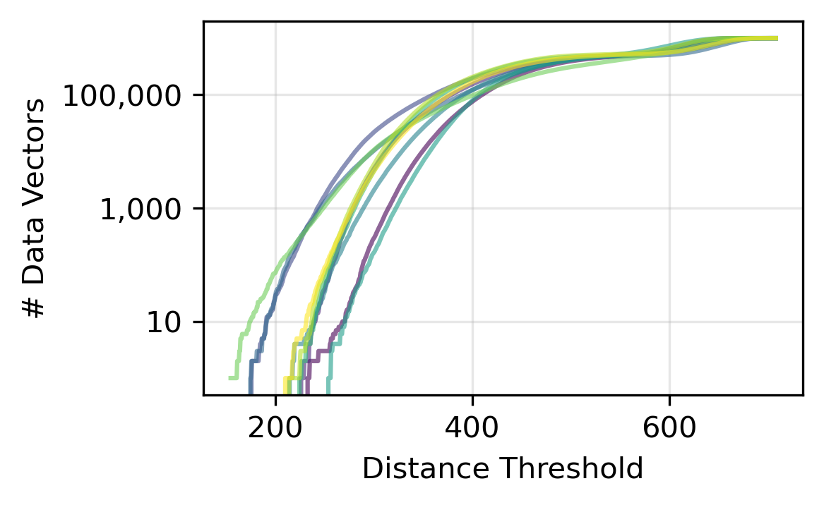
To evaluate threshold-based joins under varying selectivities, we use seven evenly spaced distance thresholds per dataset. The thresholds are chosen to cover a wide spectrum of join result sizes, from sparse joins with very few matches to dense joins where a large fraction of data vectors fall within the threshold. Table 2 reports the exact threshold values used for each dataset. Figure 10 shows the join sizes, illustrating the high variance in join sizes across both datasets and thresholds.

Note that large thresholds with large join sizes are less likely to be used in practice, similar to using small $k$ values (e.g., 5, 10, or 100) in typical top-$k$ nearest neighbor searches (Ootomo et al., 2024; Malkov and Yashunin, 2018). Therefore, we mainly focus on small thresholds (e.g., $\theta_{1}$ to $\theta_{3}$) and show the results for large thresholds for completeness.

When the threshold is large, it is often enough to estimate the join size and approximate the results as in approximate query processing (Hellerstein et al., 1997; Agarwal et al., 2013) or LIMIT the number of outputs as in exploratory data analytics (Idreos et al., 2015; Zimmerer et al., 2025), and full sequential scans or nested loop joins may be more efficient than index scans or index nested loop joins, as the selectivity increases in the relational context (Section 4.1).

Figure 9. T-SNE visualization of SIFT (left) and LAION (right), highlighting an example query (red) and it’s in-range data points (blue).

Table 2. Evenly-spaced distance thresholds ($\theta$) per dataset. We omit $\theta$ when the context is clear.

Dataset	$\theta_{1}$	$\theta_{2}$	$\theta_{3}$	$\theta_{4}$	$\theta_{5}$	$\theta_{6}$	$\theta_{7}$
SIFT	50	100	150	200	250	300	350
GIST	0.3	0.5	0.7	0.9	1.1	1.3	1.5
GloVe	0.6	0.7	0.8	0.9	1.0	1.1	1.2
NYTimes	0.1	0.3	0.5	0.7	0.9	1.1	1.3
FMNIST	500	750	1000	1250	1500	1750	2000
COCO	1.33	1.335	1.34	1.345	1.35	1.355	1.36
ImageNet	1.19	1.21	1.23	1.25	1.27	1.29	1.31
LAION	1.12	1.14	1.16	1.18	1.2	1.22	1.24

Figure 10. Join size per dataset and threshold.

5.1.2. Baselines

We implemented all baselines within our unified vector join framework (Section 3) to ensure a fair comparison and isolate the effects of work sharing and work offloading. We also implemented the state-of-the-art threshold-based vector join baseline, SimJoin (Xie et al., 2025), inside our framework and achieved similar efficiency with their paper. This allows us to fairly assess how our techniques improve over state-of-the-art work sharing.

• Naive (NLJ): A nested-loop join that computes all pairwise distances between queries $X$ and data $Y$, serving as the exact but impractical baseline.

• Index: Index nested-loop join (INLJ), where each query independently performs an approximate search over the data index.

• ES: Index with early stopping enabled (Section 4.1).

• ES+HWS: Early stopping with hard work sharing (Section 4.2), corresponding to our implementation of SimJoin (Xie et al., 2025).

• ES+SWS: Early stopping with our soft work sharing (Section 4.3).

• ES+MI: Early stopping with our merged index (Section 4.4).

• ES+MI+Adapt: Early stopping with merged index with our adaptive hybrid BBFS for OOD queries (Section 4.5).

We use the NSG graph-based index (Fu et al., 2017), following SimJoin (Xie et al., 2025), due to its strong efficiency-recall trade-off and fast convergence. Index parameters (e.g., graph degree and max queue size) are kept consistent across all methods to ensure comparability. We use the default parameters provided in (ZJULearning, 2019) with max neighborhood size of 70 and max queue size of 256.

We do not extensively tune the underlying index search algorithms beyond standard parameter settings, such as applying vector quantizations or aggressive SIMD optimizations, as our goal is to evaluate join-level optimizations rather than single-query ANN performance.

5.1.3. Metrics

We measure the latency of join execution, recall, and memory usage for the online join processing. We measure indexing time and index size for the offline phase.

5.1.4. System Configuration

For all our experiments, we use a server with Intel(R) Xeon(R) Gold 5118 CPUs and 376 GB memory. We use a single thread for evaluating vector join.

5.2. Experimental Results

5.2.1. Overall Results.

Figure 11 reports the vector join latency, global recall, and memory usage across seven distance thresholds for all eight datasets. Overall, our proposed techniques – Soft Work Sharing (SWS), Merged Index (MI), and Adaptive Hybrid BBFS (MI+Adapt) – consistently outperform the state-of-the-art baseline Hard Work Sharing (HWS, SimJoin) in both efficiency and robustness, while preserving high recall.

Naive. As expected, the nested loop join, Naive, shows consistent latency across all thresholds and gives perfect recall.

Index. The index nested loop join, Index, is significantly faster than Naive, but still exhibits high latency even for small thresholds. This is because, when threshold is small, the greedy search without early stopping traverses a large portion of index and fails to find a single in-range point. As the threshold increases, this is mitigated but the overhead of BFS increases due to the increased join size.

Using the index may drop the recall noticeably for certain datasets. For NYTimes and GIST, the greedy search cannot find an in-range point due to weak data locality. The index is weakly connected (node degrees much smaller than the other datasets, Table 1) and does not effectively navigates to existing in-range points. This also occurs for OOD scenarios (COCO, ImageNet, and LAION).

Early Stopping. ES substantially reduces the inefficiency of Index by terminating the greedy search once the best distance plateaus. ES consistently achieves orders-of-magnitude lower latency than Index at small thresholds, while maintaining comparable recall. However, ES still processes each query independently and does not reuse any traversal results across queries. As a result, its efficiency remains worse than methods that exploit work sharing.

Work Sharing. Across all datasets, ES+SWS achieves lower latency than ES+HWS, especially for small thresholds ($\theta_{1}$-$\theta_{3}$), where ES+HWS often caches no points at all and thus fails to reuse traversal efforts. By caching the closest out-range point, SWS significantly reduces the greedy search overhead for similar queries. This improvement is most visible on SIFT, GIST, GloVe, and FMNIST, where ES+SWS consistently reduces execution time by up to 3.16x compared to ES+HWS, while maintaining similar recall. For large thresholds, SWS significantly reduces the memory usage of HWS by caching the closest data node per query, not all in-range nodes.

Merged Index. ES+MI further improves performance by offloading the task of finding an initial in-range point to the offline index construction. As shown in Figure 11, MI achieves the lowest latency among all baselines across most thresholds and datasets. This effect is particularly strong for small thresholds, where the greedy search in Index, ES, ES+HWS, and ES+SWS often traverses many nodes before finding the first in-range point. With MI, the search frequently starts directly from a close data neighbor, reducing traversal overheads. Consequently, MI approaches constant-time behavior for finding an in-range point, yielding substantial speedups over ES+HWS and ES+SWS by up to 56.3x and 32.6x without sacrificing recall. Furthermore, enabling direct search from close data points often increases recall by a large margin, such as for GIST and NYTimes. Still, it often shows low recall (while higher than using separate indexes) for OOD queries. The memory usage only slightly increases compared to using separate indexes (¡ 1%).

For datasets with a significant fraction of OOD queries (COCO, ImageNet, and LAION), ES+MI+Adapt substantially improves recall by up to 43%. While vanilla BFS-based expansion can miss disconnected in-range regions for OOD queries, ES+MI+Adapt selectively activates the hybrid BBFS strategy to bridge out-range walls. As a result, ES+MI+Adapt consistently achieves higher recall than the others on these datasets with a trade-off of higher latency. Still, the latency is lower than using separate indexes (ES+SWS and ES+HWS). For the non-OOD datasets, ES+MI+Adapt achieves similar latency with ES+MI by adaptively disabling the hybrid search and falls back to the BFS (Table 1). This confirms that adaptive hybrid traversal is crucial for maintaining recall under challenging query distributions while preserving efficiency.

Figure 11. Vector join performance (latency, recall, and memory usage) on seven thresholds and eight datasets.

5.2.2. Latency-recall Trade-off.

Figure 12 presents the latency–recall trade-off when varying the maximum queue size for the smallest threshold on all eight datasets. The queue size corresponds to the parameter $L$ for Algorithms 2 and 4. For Index, ES, ES+HWS, and ES+SWS, the queue size controls the greedy search phase, while for ES+MI+Adapt, it affects the hybrid search phase. It does not affect ES+MI since the greedy phase is skipped (Section 4.4) and only performs BFS whose queue is not limited by $L$.

Index is sensitive to the queue size, where both latency and recall increase as the queue size increases. The ES baselines other than ES+MI+Adapt are insensitive to the queue size as they utilize early stopping to terminate unnecessary greedy search when the minimum distance plateaus. While ES+MI and ES+MI+Adapt together form the best Pareto curves, ES+MI+Adapt shows a clear latency-recall trade-off by controlling the hybrid queue size. This improves recall for OOD-heavy datasets by allowing controlled traversal through out-range nodes.

Figure 12. Latency-recall curves for varying queue sizes from 8 to 512. Smallest threshold, $\theta_{1}$, is used. The queue size is defined for the greedy search phase for non-MI baselines and hybrid search phase for ES+MI+Adapt.

5.2.3. Latency Breakdown.

Figure 13 breaks down the total join latency into three parts: greedy search, BFS (or hybrid BBFS), and other. As expected, Index, ES, ES+HWS, and ES+SWS are bottlenecked by the greedy search for small thresholds, finding a single in-range point, and the main goal of ES and work sharing has been to reduce the traversal effort in the greedy search in Section 4. MI avoids such overheads. BFS dominates runtime for large thresholds due to large join sizes, seeking for all in-range points.

Figure 13. Latency breakdown for FMNIST into three phases: greedy search, BFS (or hybrid BBFS), and the others. Similar results observed for the other datasets.

5.2.4. Offline Overhead.

Figure 14 compares the index size and build time of using two separate indexes – one for queries $G_{X}$ and one for data $G_{Y}$ – against merged index $G_{X\cup Y}$. Across all datasets, merged index does not introduce much overheads compared to separate indexes, because the merged index shares the same graph structure, sharing the same hyperparameters (e.g., max neighborhood size), and the total number of vectors is the same as $|X|+|Y|$. Since index construction is an offline process performed once per dataset, small additional overhead is negligible relative to the substantial runtime improvements achieved during online vector joins.

Figure 14. Offline overheads (index size and indexing time) for separate query and data indexes vs. merged index.

5.3. Scalability Test

To assess baselines under varying data scales, we vary the number of data vectors $|Y|$ using the SIFT1B dataset and the smallest threshold $\theta_{1}$, while keeping the number of queries at 10K. We vary $|Y|$ from 10K to 10M and sample $|Y|$ vectors from SIFT1B. 10M is the maximum data size we can process in memory. We leave supporting billion-scale data using multiple servers or disks as a future work. Figure 15 reports join latency as $|Y|$ increases. Recall is near 1.0 for all baselines.

Naive scales linearly with $|Y|$, as expected, since it computes all pairwise distances. Index also shows near-linear growth, because each query independently traverses a larger graph as the dataset grows. ES scales better than Index, but still exhibits noticeable growth due to repeated greedy searches. ES+HWS reduces some redundancy, but its performance degrades for large $|Y|$ due to increasing cache sizes and BFS expansion costs. ES+SWS shows improved scalability by further reducing redundant greedy search across similar queries by caching closest out-range points. ES+MI and ES+MI+Adapt achieve the best scalability, with sub-linear growth in latency by avoiding greedy search.

Figure 15. Scalability analysis on subsets of SIFT1B dataset with varying number of data vectors. The smallest threshold ($\theta_{1}$) is used.

5.4. Varying Index Type

So far, our experiments have used the NSG graph index (Fu et al., 2017) following (Xie et al., 2025). In this section, we evaluate whether our techniques generalize to a different index structure, HNSW (Malkov and Yashunin, 2018), which is also widely used in modern vector search systems (Douze et al., 2024; Wang et al., 2021).

Figure 16 compares the performance of all methods using HNSW graphs instead of NSG, on two in-distribution and out-of-distribution datasets, FMNIST and ImageNet. The relative ordering of methods remains consistent: ES+MI and ES+MI+Adapt achieve the best latency-recall trade-offs, followed by ES+SWS, ES+HWS, ES, and Index. This shows that our work-sharing and offloading techniques are index-agnostic and not tailored specifically to NSG. While we set the HNSW index sizes similar to the NSG indexes we used, in general HNSW gives lower performance (especially recall) than NSG. This supports the choice of using NSG by default in (Xie et al., 2025).

Figure 16. Vector join performance (latency, recall, and memory usage) using HNSW index (Malkov and Yashunin, 2018) on FMNIST and ImageNet.

6. Related Work

6.1. Approximate Vector Index

A wide range of index structures has been developed for single-vector queries. Early research was dominated by Locality-Sensitive Hashing (LSH) (Datar et al., 2004), which maps similar vectors into hash buckets with high probability, so queries only probe a few buckets instead of scanning all data (Jafari et al., 2021). Variants such as E2LSH (Datar et al., 2004) and C2LSH (Gan et al., 2012) trade recall for lower memory consumption and faster search.

Inverted file (IVF) and quantization-based approaches cluster the vector space into many buckets and search only a few relevant buckets per query (Baranchuk et al., 2018; Jegou et al., 2010; Guo et al., 2020). Graph-based ANN methods, such as HNSW (Malkov and Yashunin, 2018), Vamana (Jayaram Subramanya et al., 2019), and NSG (Fu et al., 2017), represent data points as nodes in a proximity graph and perform best-first search to find nearest data points, enjoying the superior efficiency-recall trade-off than the other types of indexes (Malkov and Yashunin, 2018; Fu et al., 2017; Douze et al., 2024). Our online algorithms operate on graph-based indexes but are agnostic to the specific index design.

The ANN indexes are highly optimized for single-query retrieval and are incorporated into many vector processing systems and libraries (e.g., FAISS (Douze et al., 2024) and Milvus (Wang et al., 2021)). We explore work-sharing and work-offloading mechanisms for joins in this paper that are orthogonal to such single-query optimizations, and our hybrid search only affects the online phase, thus is also orthogonal to designing new index structures.

Recently, DARTH (Chatzakis et al., 2025) proposed an early stopping mechanism for best-first search based on estimated recall using an ML model that predicts when further traversal yields diminishing returns. While effective for single-query ANN search, DARTH assumes a fixed starting point and pre-trained recall model. Such assumptions fail in the work-sharing setting, where starting points differ dynamically across queries due to reused parent results. Furthermore, it is nontrivial to apply it to our threshold-based search including BFS.

6.2. Vector Join

Early approaches for vector similarity joins act as repeated ANN selections, whereas recent research introduces join-aware optimizations. A straightforward solution is selection-based, which indexes one set for similarity search and issues queries from the other set, collecting all pairwise matches. The selection-based strategy is implicitly deployed in many systems, such as VBase (Zhang et al., 2023) and SingleStore-V (Chen et al., 2024a), but it suffers from heavy redundant work since each query traverses the index independently, even if query vectors are similar. To avoid brute-force selection, XJoin (Wang et al., 2024) reduces needless queries by skipping query vectors without neighbors within the join radius. However, XJoin still fundamentally performs a separate ANN search per query, leading to redundant computation.

Recognizing the inefficiency of per-vector searches, SimJoin (Xie et al., 2025) allows work sharing: it orders the queries along a Minimum Spanning Tree so that each query can reuse its parent’s index search path. DiskJoin (Chen et al., 2025) targets billion-scale joins on SSD-resident data, batching index accesses and orchestrating the join order to maximize data reuse from disk pages. Our method also falls into this category. Compared to SimJoin ’s hard reuse (in-range only) and DiskJoin’s I/O orchestration for disk-resident self-joins, our work advances the approximate in-memory cross-join setting with soft work sharing and a merged index.

There are distributed and parallel solutions for similarity joins. MAPSS (Wang et al., 2013) and ClusterJoin (Das Sarma et al., 2014) are MapReduce-based approximate join frameworks; specifically, MAPSS uses clustering to assign vectors to partitions and prunes comparisons via LSH, while ClusterJoin balances load and filters candidates per partition. It would be an interesting future work to extend our work sharing and offloading to disk-based, distributed, and parallel environments.

6.3. Vector Systems

Recent years have seen rapid growth of vector-native database systems that extend analytical capabilities. Milvus (Wang et al., 2021), Weaviate (Wang et al., 2021), Pinecone (28), and Qdrant (29) expose vectors as first-class data types and support top-$k$ similarity queries with integrated ANN libraries. These engines internally treat vector similarity search as a selection operator: each query vector is processed independently against an index, and multi-query workloads are executed as repeated ANN lookups.

Hybrid vector-relational systems are emerging within analytical engines. PostgreSQL extensions such as pgvector (27) allow ANN queries directly in SQL. DuckDB (Raasveldt and Mühleisen, 2019) is a lightweight in-process analytical database that includes a vector search extension. SingleStore-V (Chen et al., 2024a) integrates a vector index into its distributed relational engine and pushes similarity search to the storage nodes. While beyond the scope of this paper, one of our next steps is to deploy our ideas to such systems and measure the impact on hybrid query plans.

7. Conclusion

This paper presented a unified framework for approximate threshold-based vector joins that advances work sharing and work offloading over graph-based ANN indexes. With our soft work sharing, merged indexing, and adaptive hybrid search, the proposed techniques reduce redundant traversal and improve robustness across diverse query distributions. Extensive experimental results show significant gains in efficiency and recall compared to the state-of-the-art method, SimJoin, highlighting the importance of systematic work sharing and offloading in high-dimensional vector join processing. Future work includes extending these techniques to billion-scale datasets, adapting them to non-graph-based vector indexes, supporting streaming data, deploying them into vector or vector-relational systems, and supporting vector-relational joins with filters on the query or data side.