Locate-then-Sparsify: Attribution Guided Sparse Strategy
for Visual Hallucination Mitigation

Abstract

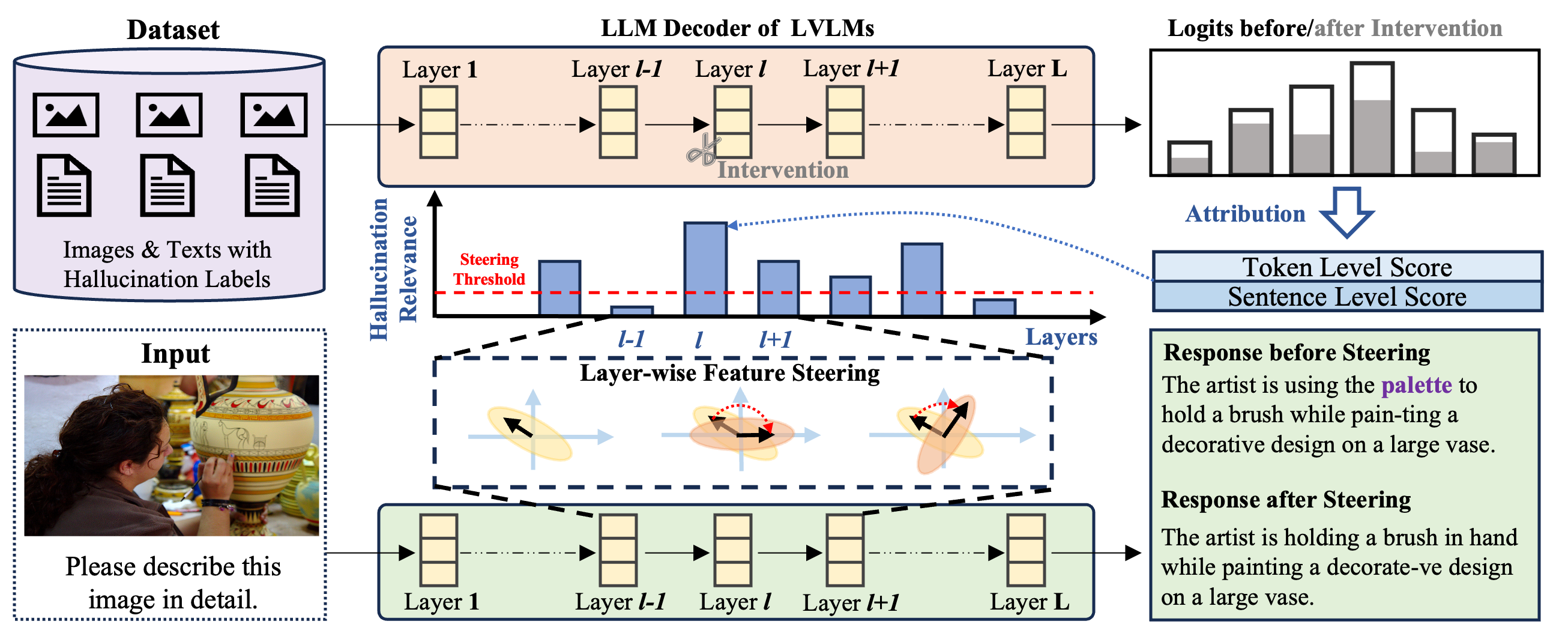
Despite the significant advancements in Large Vision-Language Models (LVLMs), their tendency to generate hallucinations undermines reliability and restricts broader practical deployment. Among the hallucination mitigation methods, feature steering emerges as a promising approach that reduces erroneous outputs in LVLMs without increasing inference costs. However, current methods apply uniform feature steering across all layers. This heuristic strategy ignores inter-layer differences, potentially disrupting layers unrelated to hallucinations and ultimately leading to performance degradation on general tasks. In this paper, we propose a plug-and-play framework called Locate-Then-Sparsify for Feature Steering (LTS-FS), which controls the steering intensity according to the hallucination relevance of each layer. We first construct a synthetic dataset comprising token-level and sentence-level hallucination cases. Based on this dataset, we introduce an attribution method based on causal interventions to quantify the hallucination relevance of each layer. With the attribution scores across layers, we propose a layerwise strategy that converts these scores into feature steering intensities for individual layers, enabling more precise adjustments specifically on hallucination-relevant layers. Extensive experiments across multiple LVLMs and benchmarks demonstrate that our LTS-FS framework effectively mitigates hallucination while preserving strong performance.

1 Introduction

By harnessing the advanced text generation capabilities of Large Language Models, Large Vision Language Models (LVLMs) have achieved impressive performance across various multimodal tasks [1, 28, 40, 44]. Despite their strong performance, LVLMs face a significant challenge known as hallucination, wherein the model generates fluent and semantically coherent responses that include factually incorrect statements about the input visual content [21, 12, 44]. Such hallucinations hinder the reliability of LVLMs, posing serious risks in real-world applications [16, 34].

(a) TSNE visualizations of features in LVLM layers.

(b) Performance on CHAIR and MMMU benchmarks.

Figure 1: Current methods (e.g., Nullu [42]) mitigate hallucinations by uniformly steering features across layers, which (a) alters feature distributions and (b) leads to degraded performance on general tasks like MMMU. In contrast, we propose a layerwise steering framework, LTS-FS, which mitigates hallucinations more effectively (e.g., on CHAIR) while minimally perturbing the feature distributions, thus preserving more generalization ability.

To mitigate hallucinations in LVLMs, early studies finetune the whole model on specially designed datasets, which is costly and degrades its generalization ability [25, 38, 9]. In contrast, decoding-based methods introduce strategies such as contrastive decoding [19, 2] and self-correction [45, 5] to mitigate hallucinations in a training-free manner, thereby preserving the original capabilities of pre-trained models. Nevertheless, these methods significantly increase the number of decoding steps required for each input query, leading to high inference costs for real-world deployment.

Recently, feature steering methods [42, 31] show promise to overcome the above limitations. These methods adjust features of intermediate layers by steering them from their original positions in the feature space toward directions that are less prone to generating hallucination outputs. By modifying only the features without introducing additional decoding steps, feature steering methods can maintain inference costs comparable to those of the original model. However, current methods steer features based on heuristically designed rules [31] (e.g., adjust all layers). These rules overlook the inherent differences across layers in pre-trained models, making the steering process to disturb layers less relevant to hallucinations. The disruption alters the distributions of features(in  Fig. 1(b)) and ultimately impairs the model’s generalization ability (in Fig. 1(a)), similar to the tuning-based methods. Therefore, an upgraded method to mitigate hallucinations that can achieve feature steering while preserving the original capabilities of LVLMs is urgently required.

In this paper, we propose Locate-Then-Sparsify for Feature Steering (LTS-FS), a plug-and-play framework that effectively mitigates hallucinations while preserving the inherent capabilities of LVLMs. First, we construct a dataset including hallucination samples at two granularities. With this dataset, we locate the hallucination-relevant layers through intervention-based attribution. Guided by the attribution score, we propose a layerwise strategy that selectively steers features in hallucination-relevant layers rather than uniformly adjusting all layers. As shown in Fig. 1, compared with Nullu, a classical feature-steering-based method, our strategy barely disrupts the original feature distribution. Meanwhile, the evaluation results on the MMMU benchmark demonstrate that our LTS-FS not only maintains fewer hallucinatory expressions but also achieves better generalization performance.

Specifically, for dataset construction, we first distinguish hallucinations in LVLMs according to token-level and sentence-level granularities. Then, we construct hallucination samples at token and sentence granularity levels to build a dataset. Supported by this dataset, we locate hallucination-relevant layers through an attribution method based on causal interventions. This method sequentially masks the attention output of each layer to assess its contribution to the logits of hallucination outputs. Based on the contribution, we define attribution scores and assign them to each layer, which reflects its relevance to hallucination phenomenon. After obtaining layer-wise attribution scores, we propose a sparsity-aware layer selection and steering strategy that converts the attribution scores into steering intensities (i.e., applying weaker steering to layers with low scores and stronger steering to those with high scores). By modifying only hallucination-relevant layers, we mitigate hallucinations while minimizing interference with the model’s feature distribution, thereby more effectively preserving its original capabilities. We conduct extensive experiments to demonstrate that LTS-FS can further improve the hallucination mitigation capacity of current SOTA feature steering methods (e.g., 2% accuracy gain on POPE-popular with Qwen-VL-2.5-7B) while preserving more generalization capability of LVLMs (e.g., increasing detailness from 4.72 to 4.92 under GPT4v Aided Evaluation on LLaVA-Bench). Codes are available at https://github.com/huttersadan/LTS-FS.

• We introduce a granularity-based hallucination categorization and construct a synthetic dataset to correlate model components with hallucinations.

• We employ an intervention-based attribution method to locate hallucination-relevant layers by quantifying their contributions to hallucination outputs.

• We propose a layerwise strategy that selectively adjusts steering intensity, achieving SOTA hallucination mitigation results while preserving the generalization ability.

2 Related Work

2.1 Hallucinations in LVLMs

Hallucinations have been extensively studied in the artificial intelligence community. Many studies have been carried out with the aim of reducing the impact of hallucinations [17, 13, 48, 26]. Hallucinations in LVLMs refer more to the mismatch between the visual and textual content modalities. Most methods are based on self-correction [45, 5], instruction-tuning [38, 25, 9], or decoding-enhancement [14, 19, 2]. Typically, Yin et al. [45] refined textual responses while correcting hallucinations. Liu et al. [25] composed negative instances to refrain from over-confidence. Huang et al. [14] penalized specific tokens during decoding, which suppresses the formation of hallucinations. These methods generally require a large amount of manually labeled data and computing resources or suffer longer inference times. To avoid these limitations, recent studies have proposed feature steering methods [42, 31, 20]. Yang et al. [42] projected generated captions into a dedicated space to suppress hallucinated entities. Liu et al. [31] proposed an intervention-based approach, steering the latent representations during inference with a pre-computed “anti-hallucination” direction. However, directly adjusting weights or features may hinder the internal knowledge and suffer a reduction in generalization ability. To overcome these limitations, our method identifies hallucination-relevant layers and selectively adjusts features within them, thereby better preserving the internal knowledge of LVLMs.

2.2 Parameter Localization

Parameter localization, a technique that identifies parameters correlated with specific datasets, offers flexible and effective solutions for downstream tasks such as model fine-tuning [36], knowledge editing [30], and model compression [39]. According to localization granularity, existing localization methods can be categorized into weight-level [11] and layer-level [7] paradigms. For the weight-level paradigm, current methods design specific rules such as activations [11], redundancy [37], second derivatives [8], and energy efficiency [43] to locate the data-relevant weights. For the layer-level paradigm, GRIFFIN [7] selects layers based on their high activation magnitudes in response to input prompts. FLAP [3] computes the sample variance of each input feature as importance and locates layers accordingly. RL-Pruner [39] determines the layer-wise importance distribution through reinforcement learning. Unlike the above methods designed for pruning or adjusting model parameters, we employ a layer-level strategy to locate the layers relevant to the hallucination phenomenon in LVLMs. The localization results can effectively support the feature steering process to mitigate hallucinations.

2.3 Sparse Adjustments for Pre-trained Models

To enhance the model capability in a specific domain while minimizing unintended disruptions to the overall model behavior, researchers have proposed sparse adjustment methods [30, 18, 32, 23] that selectively modify a subset of model components. NMKE [30] sparsely updates hidden neurons to edit the internal knowledge in LLMs. Jia et al. [18] develop a sparsity-aware method for model unlearning. BNS [32] selectively suppresses neuron activations to mitigate the social bias in pre-trained language models. Their sparse selection strategies are typically neuron-wise and designed for specific parameter adjustment methods [30]. In contrast, we propose a layer-wise sparse selection strategy to enhance the feature steering paradigm for hallucination mitigation. This strategy is decoupled from any particular steering method, delivering consistently improved performance across different steering methods.

3 Method

In this section, we first construct the bi-granularity hallucination dataset (Sec. 3.1). Based on this dataset, we introduce causal attribution to locate hallucination-relevant layers (Sec. 3.2) and employ a layerwise sparse selection scheme to mitigate hallucination while maintaining the generalization ability of LVLMs (Sec. 3.3).

3.1 Bi-granularity Dataset Construction

For locating hallucination-relevant layers, we build a bi-granularity dataset by constructing hallucination samples at the token level and sentence level according to their text length. Specifically, for single-sentence texts, their hallucinations can be annotated at the token level based on existing hallucination benchmarks [21, 41]. However, for multiple-sentence texts, token-level annotation is insufficient. As the length of generated text increases, the model’s behavior evolves from producing isolated hallucinatory tokens to generating entire hallucinatory sentences (i.e., removing them can significantly enhance the factuality with minimal impact on generation quality) [14]. Therefore, we categorize these samples as the sentence level for comprehensive localization of hallucination-relevant layers.

The bi-granularity hallucination samples are constructed based on current hallucination benchmarks: CHAIR [33], POPE [22], Antidote [41]. Token-level samples are typically constructed by prompts phrased as wh-questions or yes/no questions. POPE and Antidote benchmarks contain such types of questions. Moreover, hallucination tokens can be identified by rule-based methods. For sentence-level hallucinations, we split multi-sentence texts and assess the image-grounded consistency of each sentence based on CHAIR, which is effective in identifying hallucination tokens. Sentences containing such tokens are labeled as hallucinatory. More details are presented in the supplementary.

Figure 2: Hallucination examples at token level and sentence level.

Examples of Both Granularities. At the token level, as shown in Fig. 2 (a), the model generates a short response to a specific interrogative about a given item. In such cases, not all tokens are hallucinatory. Only “the palette” is absent from the image, while the remaining tokens describe objectively present content. At the sentence level, for longer and free-form responses in Fig. 2 (b), the red part of the text reflects content conjectured from prior text and the image. The entire clause following “reflection” is unsupported.

Figure 3: Overview of our LTS-FS framework. First, we build a bi-granularity dataset with token level and sentence level hallucinations. Then, based on the dataset, hallucination-relevant layers are located through intervention-based attribution. Finally, a layerwise strategy is applied to control the feature steering intensity across layers according to the attribution scores.

Data Usage and Split Protocol. Note that all samples used to locate hallucination-relevant layers are computed only on the training split (or a small calibration subset drawn from it) and do not include any samples from the evaluation benchmarks. Once the dataset is constructed, the subsequent policy is fixed and consistently applied to all following test evaluations without modification.

3.2 Hallucination-Relevant Layer Localization

After constructing a dataset including images and texts annotated with hallucination labels, we utilize it to locate the LVLM layers that are more prone to inducing hallucination (i.e., hallucination-relevant layers). Inspired by prior studies [46, 47], we design an attribution method that estimates the relevance between hidden layers of LVLMs and logits of hallucination outputs through causal intervention.

Feed-Forward Process in LVLM Layers. Consider an LVLM composed of an image encoder, a projection module, and an LLM with $L$ layers. In the LLM decoding process, the output feature $\mathbf{h}_{l}$ of layer $l$ is calculated as follows:

$$\mathbf{a}_{l}=\texttt{MultiHeadAttn}(\mathbf{h}_{l-1},h),$$ (1)

$$\mathbf{x}_{l}=\texttt{MLP}\big(\texttt{LN}(\mathbf{h}_{l-1}+\mathbf{a}_{l})\big),$$ (2)

$$\mathbf{h}_{l}=\texttt{LN}(\mathbf{x}_{l}+\texttt{LN}(\mathbf{h}_{l-1}+\mathbf{a}_{l})).$$ (3)

Here, $\mathbf{a}_{l}$ and $\mathbf{x}_{l}$ are the outputs of the multi-head attention (MHA) and MLP, respectively. LN denotes the LayerNorm module. The MHA output $\mathbf{a}_{l}$ concatenates the output of $H$ heads. Given the output feature $\mathbf{h}_{l-1}$ at layer $l-1$, the attention output $\mathbf{a}_{l}$ and the parameters in subsquent layers $\theta_{\geq l}$, the logits of token $y$ is predicted as follows:

$$y\sim P_{\theta_{\geq l}}\big(y\mid\mathbf{h}_{l-1},\mathbf{a}_{l}\big).$$ (4)

Layer-wise Attribution. To locate hallucination-relevant layers, we measure their contributions to hallucination outputs by introducing attribution scores at the token level and sentence level based on causal intervention techniques. Given the MHA output $\mathbf{a}_{l}$ of layer $l$, and the output feature of the prior layer $\mathbf{h}_{l-1}$. The attribution score at the token level $s_{\text{tok}}^{l}$ of layer $l$ is calculated as:

$$s_{\text{tok}}^{l}=\sum_{h=1}^{H}\log\left(\frac{P_{\theta_{\geq l}}(y\,\big|\mathbf{h}_{l-1},\mathbf{a}_{l})}{P_{\theta_{\geq l}}(y\,\big|\mathbf{h}_{l-1},\mathbf{a}_{l}\odot M^{h})}\right).$$ (5)

$M^{h}$ denotes a mask that sets the output of the $h$-th attention head to zero. We independently intervene on attention heads to measure the relevance between layers and hallucinatory tokens, building on prior studies [47, 49] that such interventions enable more accurate estimation of how individual layers contribute to the logits of output tokens.

For the sentence level, we compute the attribution scores across all tokens in the sentence and aggregate them to obtain an overall attribution score, as the entire sentence is intrinsically associated with the hallucinated content [14, 49]. Since individual tokens vary in their contribution to hallucinations, we employ a weight-based aggregation method that assigns token weights according to several indicators, which are designed based on insights from prior studies [14, 49]. These studies suggest that (1) initial summarizing cues (e.g., additional) or the terminal punctuation of the preceding sentence and (2) later tokens in the sentence, are more likely to trigger hallucination. Furthermore, (3) tokens exhibiting factual errors should also be emphasized. Therefore, we design three indicators to assign these tokens with higher weights. Given the set of tokens $T_{sent}$ in a sentence, the indicators for a token $y_{t}\in T_{sent}$ is defined as follows:
(1) Cue indicator: $u(y_{t}|T_{sent})\in\{0,1\}$, where $u(y_{t}\mid T_{sent})=1$ if $y_{t}$ is a summary token (e.g., “additional” or a period); otherwise $u(y_{t}\mid T_{sent})=0$.
(2) Position indicator: $r(y_{t}|T_{sent})\in[0,1]$, a higher value indicates later positions in the sentence.
(3) Hallucination indicator: $v(y_{t}|T_{sent})\in\{0,1\}$, where $v(y_{t}|T_{sent})=1$ if the token $y_{t}$ is identified as containing a factual error, and $v(y_{t}|T_{sent})=0$ otherwise.
A multiplicative weight is formed and then normalized:

$$\tilde{w}(y_{t}\mid T_{sent}) =(1+\lambda_{\mathrm{cue}}\,u(y_{t}\mid T_{sent}))$$ (6)

$$\times(1+\lambda_{\mathrm{pos}}\,r(y_{t}\mid T_{sent}))$$

$$\times(1+\lambda_{\mathrm{hall}}\,v(y_{t}\mid T_{sent})),$$

$$w(y_{t}\mid T_{sent}) =\frac{\tilde{w}(y_{t}\mid T_{sent})}{\sum_{y_{k}\in T_{sent}}\tilde{w}(y_{k}\mid T_{sent})},$$

where $\lambda_{\mathrm{pos}},\lambda_{\mathrm{cue}},\lambda_{\mathrm{hall}}\!\geq\!0$ are hyperparameters that control the strength of the three indicators. The attribution score for sentence-level hallucinations at layer $l$ is computed as the weighted sum of the token level attribution scores $s_{tok}^{l}$.

$$s_{\text{sent}}^{\,l}=\sum_{y_{t}\in T_{sent}}w(y_{t}\mid T_{sent})\cdot s_{tok}^{\,l}.$$ (7)

In practice, attribution scores are utilized according to specific tasks. For simple tasks such as question answering, token-level score is employed due to the conciseness of model outputs. In contrast, sentence-level score is adopted in more general tasks such as image captioning.

3.3 Layerwise Feature Steering

After locating hallucination-relevant layers with higher attribution scores, an intuitive approach is to apply feature steering exclusively to these layers. In contrast to existing feature steering methods that uniformly steer all layers, layer-wise steering enables more targeted hallucination mitigation while minimizing unnecessary interference with the LVLM’s internal representations.

Specifically, we propose a layer-wise steering strategy that combines hard sparsification and soft weighting. For layers with extremely low attribution scores, steering features of these layers has minimal impact on mitigating the model’s hallucinations while substantially impairing its generalization capability. Therefore, we exclude such layers from the steering process by employing a mask parameterized by a threshold $r_{s}$.

For layers with high attribution scores, we scale the steering intensity proportionally to their normalized attribution scores $\tilde{s}^{l}$ (i.e., features in higher-scoring layers are steered more strongly). The soft weighting achieves a more favorable balance between mitigating hallucinations and preserving the model’s generalization capability.

The detailed implementation of our layer-wise steering strategy is presented in Algorithm 1. Since we only adjust the intensity of steering, our method can be seamlessly integrated into existing feature steering methods [31, 42], as all of them inherently require an explicit setting of steering intensity. Moreover, given a fixed pre-trained LVLM, the layer-wise intensity derived by our framework is generalizable across diverse steering methods, highlighting the broad applicability and strong reusability of our framework.

Algorithm 1 Feature Steering at layer $l$

0: layerwise attribution score $s^{l}$, mask threshold $r_{s}$, initial feature steering intensity $\lambda$, output features $\mathbf{h}_{l}$, and feature steering function $f:\mathbb{R}^{d}\times\mathbb{R}\rightarrow\mathbb{R}^{d}$.

0: steered feature $\tilde{\mathbf{h}}_{l}$

1: Computing threshold: $\tau=r_{s}\cdot\frac{1}{L}\sum_{l=1}^{L}s^{l}$

2: Constructing mask: $m_{l}=\mathbf{1}\!\left[s^{\,l}\geq\tau\right]$

3: Masking attribution score $s^{l}=m_{l}\cdot s^{l}$

4: Normalizing attribution score $\tilde{s}^{l}=\frac{s^{l}}{\sum_{i=1}^{L}s^{i}}$

5: Scaling feature steering intensity $\lambda_{l}=\lambda*m_{l}+\lambda\cdot\tilde{s}_{l}$

6: Steering feature $\tilde{\mathbf{h}}_{l}=f(\mathbf{h}_{l},\lambda_{l})$

7: return $\mathbf{h}_{l}$

4 Experiments and Analysis

In this section, we empirically investigate the effectiveness of LTS-FS in mitigating hallucinations while preserving model generalization. Remarkably, we use 100 sentence-level hallucination samples and 100 token-level hallucination samples to synthesize the Bi-granularity dataset for layer-wise attribution. The sentence-level hallucination samples are selected and processed from CHAIR benchmark [33], while the token-level hallucination samples are from POPE [22] and Antidote [41].

Table 1: CHAIR results of various LVLMs on MSCOCO. Bold indicates the best performance. C_S and C_S mean lower hallucination. Recall and output length (Len.) serve as controls, indicating that reductions in C_S/C_I do not stem from suppressing objects or truncating responses. ^∗ denotes the feature steering methods.

Method	LLaVA-v1.5-7B				LLaVA-v1.5-13B				Qwen-VL2.5-7B
	CS$\downarrow$	CI$\downarrow$	Recall	Len.	CS$\downarrow$	CI$\downarrow$	Recall	Len.	CS$\downarrow$	CI$\downarrow$	Recall	Len.
Regular	53.0	13.9	77.2	98.0	40.8	9.5	77.2	111.8	27.0	7.4	61.6	120.6
VCD	55.2	16.7	77.5	89.2	39.2	9.2	79.1	108.2	26.2	7.6	61.2	120.3
AGLA	50.8	16.1	75.2	88.1	38.4	9.1	78.7	109.3	25.2	7.1	59.5	118.6
$\text{Nullu}^{*}$	50.2	13.7	76.9	93.3	38.0	9.4	74.5	105.8	27.4	7.7	60.7	121.6
$\text{VTI}^{*}$	47.4	13.9	76.2	88.9	36.3	9.2	75.9	94.4	25.5	7.1	61.6	121.3
LTS-FS (Nullu)	46.8	13.5	76.6	93.2	35.7	8.9	76.1	109.8	23.8	6.0	60.8	120.6
LTS-FS (VTI)	35.8	11.9	75.4	82.2	32.0	8.8	74.2	83.6	24.8	6.6	62.5	120.0

Table 2: Comparison of the average accuracy under different settings (i.e., Random, Popular, Adversarial) with different baselines and our framework on POPE Bold indicates the best results, and underline means the second bests. ^∗ denotes the feature steering methods.

Method	LLaVA-v1.5-7B			LLaVA-v1.5-13B			Qwen-VL2.5-7B
	Popular	Random	Adversarial	Popular	Random	Adversarial	Popular	Random	Adversarial
Regular	77.52	85.37	70.13	78.40	81.91	71.07	83.31	85.32	80.17
VCD	79.09	86.55	71.48	79.38	82.27	71.73	83.19	85.94	80.56
AGLA	78.67	85.32	71.63	80.11	82.64	72.27	83.34	86.02	80.92
$\text{Nullu}^{*}$	79.42	86.35	71.57	80.88	83.24	72.43	83.06	85.82	80.74
$\text{VTI}^{*}$	77.03	84.84	69.40	79.22	84.08	71.77	82.74	85.49	80.19
LTS-FS(Nullu)	80.09	87.13	72.62	81.46	83.96	73.06	83.59	86.21	81.11
LTS-FS(VTI)	79.96	86.77	73.04	81.77	86.59	73.78	83.35	86.04	80.92

Table 3: Comparison of the average F1 score under different settings (i.e., Random, Popular, Adversarial) with different baselines and our framework on POPE. Bold indicates the best results, and underline is the second best. ^∗ denotes the feature steering methods.

Method	LLaVA-v1.5-7B			LLaVA-v1.5-13B			Qwen-VL2.5-7B
	Popular	Random	Adversarial	Popular	Random	Adversarial	Popular	Random	Adversarial
Regular	80.71	86.47	75.85	81.30	83.85	76.47	81.68	83.54	78.93
VCD	81.23	87.16	76.04	82.01	83.76	75.76	81.95	83.88	79.51
AGLA	81.47	86.77	75.89	82.32	83.58	75.48	81.86	83.63	79.14
$\text{Nullu}^{*}$	81.67	86.28	76.17	82.97	84.73	77.04	81.27	83.73	79.32
$\text{VTI}^{*}$	80.40	86.08	75.42	81.83	83.82	76.80	80.88	83.37	78.70
LTS-FS(Nullu)	82.20	87.64	76.22	83.42	85.56	78.36	82.55	84.31	79.83
LTS-FS(VTI)	82.25	87.32	77.32	83.58	87.48	79.91	81.38	83.88	79.46

4.1 Benchmarks and Baselines

Benchmarks. Following prior work, we evaluate our LTS-FS on typical benchmarks CHAIR [33] and POPE [22]. Each metric was averaged across three independent runs with distinct random seeds. To assess overall performance after feature steering, we further include experiments on MME [10] and LLaVA-Bench [27].

(a) CHAIR: Caption Hallucination Assessment with Image Relevance [33] is a widely used benchmark to evaluate object hallucination in image captioning. It quantifies the degree of object hallucination by calculating the ratio of all mentioned objects in the generated text that are not in the ground truth object set. There are two assessment criteria. CHAIR_S quantifies the degree of object hallucinations at the sentence-level, while CHAIR_I focuses on the instance level. Lower C_S and C_I indicate fewer hallucinations. In addition, we also report Recall and Sentence Length to ensure a fair comparison, since the reported hallucination metrics may be affected by the amount of generated content.

(b) POPE: Polling-based Object Probing Evaluation [22] contains 27,000 question-answer pairs about objects in MSCOCO [24], A-OKVQA [35], and GQA [15]. These question-answer pairs involve only yes/no questions and are evenly distributed among existing and absent objects. There are three negative sample settings in each dataset, i.e., random, popular, and adversarial [22]. This benchmark is evaluated by classification, with the metrics of Accuracy, Recall, Precision, and F1-Score.

(c) MME: Multi-modal Large Language Model Evaluation [10] is a comprehensive evaluation benchmark for LVLMs that assesses their perception and cognition abilities. It comprises ten perception-related and four cognition-related tasks evaluated by binary classification. MME is employed to measure hallucination while also capturing aspects of general model ability.

(d) LLaVA-Bench: LLaVA-Bench [27] comprises 24 images, each accompanied by a detailed, manually crafted description and a set of meticulously selected questions. Although this collection is relatively small in scale, it poses greater challenges for LVLMs. We use GPT-4v to evaluate the model’s generations, assessing general capability.

Baselines. We integrate our framework with two feature steering methods, Nullu [42] and VTI [31]. To validate the utility of our methods, we evaluate the effectiveness of these two models, LTS-FS (Nullu) and LTS-FS (VTI), on three mainstream large vision-language models, including LLaVA-v1.5-7B [29], LLaVA-v1.5-13B [29] and Qwen-vl2.5-7B [4]. We compare our method with state-of-the-art baselines: VCD [19], AGLA [2], Nullu [42], and VTI [31].

Implementation: For other hallucination mitigation methods, we use the default settings. In our methods, we set $\lambda_{\mathrm{pos}}=1$, $\lambda_{\mathrm{cue}}=1$, $\lambda_{\mathrm{hall}}=1$, and $r_{s}=0.5$. More detailed implementation details can be found in the Appendix.

4.2 Results on CHAIR

In CHAIR evaluation, we use Please describe the image in detail as the prompt. The results shown in  Tab. 1 confirm that our LTS-FS consistently outperforms the evaluated methods. The lowest CHAIR_S and CHAIR_I indicate our framework can better integrate visual knowledge and effectively reduce hallucinations. Comparison with Nullu and VTI demonstrates that our strategy can further enhance the performance of feature-steering-based methods. Moreover, the Recall and Length of our method are comparable to those of other methods. This provides partial evidence that our method mitigates hallucinations without sacrificing generation quality. For the evaluation of text generation quality, we have provided additional results in Appendix 9.

Inference Time Analysis. Compared with decoding-based methods (VCD and AGLA), feature-steering-based methods (Nullu and VTI) do not involve time-consuming additional processes in inference; thus, the inference speed is similar to that of the regular setting. Our framework also inherits this favorable characteristic. Detailed analysis can be found in Appendix 12.

Figure 4: Results of MME evaluation.

4.3 Results on POPE

We conduct evaluations on POPE benchmark under the Popular, Random, and Adversarial settings. Here, we mainly provide the average results of Accuracy and F1-score, respectively shown in Tab. 2 and Tab. 3. The comprehensive results can be found in the Supplementary Materials. Since we use Qwen-VL for evaluation, some methods (e.g., Nullu) did not report corresponding results. Therefore, we reproduce all methods under as consistent an environment as possible to ensure fair comparison.

Experiments show that our method achieves the best accuracy and F1-score under all settings. Particularly, when using LLaVA-v1.5-13B, it increases the accuracy of the Random setting from 81.91% to 86.59%. The results demonstrate the effectiveness of LTS-FS in mitigating hallucinations and its broad applicability across diverse open-source LVLMs and datasets.

4.4 Results on MME

We present the results of LLaVA-1.5-7B on MME benchmark as a representative to evaluate the general ability of the edited model. As shown in Fig. 4, we can observe that LTS-FS consistently achieves enhanced performance across all perception-related tasks in MME. It is worth noting that Nullu achieves significant improvements mainly in tasks such as OCR and Posters, but has negligible effects in some tasks (e.g., Count). This likely indicates that typical feature-steering-based methods are susceptible to changes in feature distribution, whereas our layer-wise strategy can better ensure the comprehensive capability of the model. More details are provided in Appendix 11.

Table 4: Ablation results for different granularity levels.

Hallucination Level	CS	CS	POPE acc	POPE f1
Baseline (Nullu)	50.2	13.7	79.11	81.37
Token-level only	50.0	13.4	79.59	81.85
Sentence-level only	47.3	13.0	79.33	81.58
Both level	46.8	13.5	79.92	82.02

Table 5: Ablation results for different choices of $r_{s}$.

$r_{s}$	CHAIRS	CHAIRS	Recall	Length
0.0 (Regular)	53.0	13.9	77.2	98.0
0.3	49.5	14.2	76.2	95.7
0.5	46.8	13.5	76.6	93.2
0.7	47.6	13.0	76.6	97.0
0.9	49.1	13.3	75.7	96.8
Soft Gating	46.7	13.4	76.1	94.5

Figure 5: Demonstration of our framework for hallucination mitigation on two examples of LLaVA-Bench using LLaVA-v1.5-7B.

4.5 Ablation Studies

Effect of Two Granularity Hallucination Levels. We discuss the effect of different granularity hallucination levels by respectively evaluating LTS-FS on the sub-datasets with only token-level hallucination and only sentence-level hallucination. Results are shown in Tab. 4, regarding the performance of Nullu as baseline. “Token-level only” setup refers to calculating the attribution scores only based on token-level hallucination samples in the layer localization process. In contrast, the ”Sentence-level only” setup is only based on sentence-level hallucination samples. “Both level” setup is equivalent to the overall framework of LTS-FS.

Results on the CHAIR benchmark indicate that layer localization based on sentence-level hallucinations achieves a more significant mitigation effect. This further demonstrates that sentence-level hallucination attribution is particularly beneficial for longer outputs, which is also consistent with intuitive expectations. In contrast, layer localization based on token-level hallucinations is more adaptable to the short responses in POPE. However, the ”Both level” setup achieves the optimal performance in the POPE evaluation, which indicates that integrating sentence-level attribution is more conducive to enhancing the model’s robustness. Combining hallucination samples at the two granularity levels can expand the conceptual range of hallucination attribution, thereby enabling more precise layer-wise localization.

Selection of Mask Threshold $r_{s}$. The hyper-parameter $r_{s}$ directly determines how many layers should be steered. We compare the results on the CHAIR across a set of candidate $r_{s}$-values to discuss the impact of the mask threshold on generation performance. The LVLM is LLaVA-v1.5-7B, and the feature-steering basis method is Nullu. As shown in Tab. 5, our strategy consistently enhances the hallucination mitigation effect. Meanwhile, the differences in results caused by $r_{s}\in[0.5,0.7]$ are negligible, which indicates that non-extreme selections of $r_{s}$ are sufficient to improve the performance of the feature steering method.

We also investigate a soft gating variant for selecting $r_{s}$. Compared with fixing $r_{s}$ for all samples, soft gating sets $r_{s}$ per sample based on the attribution-score distribution across layers, allowing the number of steered layers to vary with the input. As shown in Tab. 5, soft gating performs comparably to hard gating with negligible differences, so we use hard gating with a fixed $r_{s}$ in all experiments for simplicity.

Table 6: GPT-4V-aided evaluation of LLava-Bench.

Model	Method	Accuracy$\uparrow$	Detailedness$\uparrow$
LLaVA-1.5	Original	5.74	5.23
	Nullu	6.46	5.51
	LTS-FS(Nullu)	6.96	6.23
Qwen-vl2.5	Original	6.06	5.54
	Nullu	6.37	5.68
	LTS-FS(Nullu)	6.59	6.07

4.6 Further Analysis

Case Study on LLava-Bench. In Fig. 5, we provide two case studies based on LLaVA-v1.5-7B. The examples show clearly that hallucinations still exist in typical feature-steering methods, where nonexistent details such as “cut-in-half sandwiches”, “pirate ships”, and “pirate hats” are fabricated. Our method consistently avoids these errors and produces descriptions that remain faithful to the visual content. These qualitative results demonstrate that our layer-wise feature steering effectively suppresses hallucinations while better preserving the comprehensive capabilities of the model and the fluent presentation.

GPT-4V Aided Evaluation on LLaVA-Bench. Following Nullu [42], we evaluate the performance of our method using GPT-4V Aided Evaluation. The results are shown in Tab. 6, which demonstrates that our method can mitigate hallucination while better maintaining generation ability.

5 Conclusion

In this paper, we propose a plug-and-play framework called Locate-Then-Sparsify for Feature Steering (LTS-FS), which can mitigate hallucinations for LVLMs through feature steering while better preserving their generalization ability. We first construct a bi-granularity hallucination dataset. With this dataset, we attribute hallucination-relevant layers based on causal interventions. Finally, we design a layerwise strategy to selectively control the steering intensity according to the attribution scores across layers. Extensive experiments demonstrate that LTS-FS can effectively mitigate hallucinations while preserving the generalization ability of LVLMs. For future work, we will investigate the characteristics of hallucination-relevant layers detected by LTS-FS and try to integrate LTS-FS framework into the model pre-training process to more fundamentally reduce the generation of hallucinations.

Acknowledgement This work was supported in part by National Natural Science Foundation of China: 62236008, and in part by the Natural Science Foundation of Beijing under grant number L251082. The authors would like to thank all the anonymous reviewers for their insightful comments.

Supplementary Material

6 Details of the construction of the dataset

In this section, we introduce the details of how to construct the Bi-granularity Dataset.

At first, to preserve generalization, the data used for dataset construction and the data used for experiments are strictly disjoint. Particularly, for data selected based on CHAIR and POPE, we use data from train spilt of MSCOCO. for data selected from Antidote, we do not use these data for evaluation.

Secondly, we explain how to get a single data. As an example from CHAIR, the data instance is generated by an LVLM. We use LLaVA-v1.5-7B to produce a response according to the CHAIR benchmark, as illustrated in Fig. 6. We then apply CHAIR’s evaluation criteria to detect hallucination and annotate the instance under our two-level scheme (token- and sentence-level). And then a piece of data is generated. If the responses doesn’t have hallucination, there are just not selected.

Finally, for balance two level of data, we select 100 sentence-level samples and 100 token-level samples. All data are manually inspected to ensure accuracy.

7 Implementation details of LTS-FS

Hyper-parameters. The strength control parameters of $s^{l}_{tok}$: $\lambda_{cue},\lambda_{pos},\lambda_{hall}$ is set to be 1. The mask threshold $r_{s}$ is selected to be 0.5, as shown in Tab.5 of main text.

Environment. All the experiments are conducted on one A100 80G. For 7B model, two RTX3090 24G can replace A100. For detailed python requirements, please refer to our released codes.

8 Implementation Settings of CHAIR Results

Generation Setting. Here we set the generation config as follows: Max_New_Tokens=128, num_beams=1, and sampling=False.

Compared methods. We employ the default parameters and settings as reported in the original papers.

9 Generation Capability.

To evaluate general capability more comprehensively, we perform an evaluation using a broader benchmark called CLAIR [6]. This result in Tab. 7 shows that LTS-FS achieves a better trade-off between hallucination mitigation and general capability preservation.

Table 7: Trade-off between hallucination mitigation and general capability preservation.

Method	CHAIRs	POPE acc	details	CLAIR
Original	53.0	77.63	5.23	80.03
nullu	50.2	79.11	5.51	75.00
LTS-FS(nullu)	46.8	79.92	6.23	82.74
Soft Gating	46.7	79.5	6.26	83.64

10 More details of POPE results

Generation Setting. Here we set the generation config as follows: Max_New_Tokens=16, num_beams=1, and sampling=False.

Compared methods. We employ the default parameters and settings as reported in original papers.

Total Results. The total results is shown in Tab. 13. Across all settings, our LTS-FS framework achieves the best accuracy and F1, demonstrating consistent effectiveness in hallucination mitigation. Compared with the original feature-steering methods, applying LTS-FS consistently improves both VTI and Nullu on hallucination-related metrics. Although LTS-FS and the other methods trade wins on recall, LTS-FS consistently maintains higher precision. Since, in hallucination evaluation, precision is more indicative of mitigation quality, this further supports the strong performance of our approach.

11 More details of MME results

We report the MME numerical results in Tab. 8. The numerical results demonstrate that LTS-FS can strongly increase the mitigation abilitity of feature steering methods. Specifically, across the subset most related to hallucination: Count, and Position, LTS-FS achieves great improvements, highlighting its effectiveness in enhancing feature-steering–based mitigation.

MME includes not only perception-related tasks but also recognition-related tasks. We report these results in Tab. 9. Despite the sparsity selection emphasizes hallucination related cues rather than recognition factors, LTS-FS still produces improvements on recognition-related tasks.

Table 8: Results on all MME perception-related tasks.

Method	Existence	Count	Position	Color	Posters	Celebrity	Scene	Landmark	Artwork	OCR	Total
Regular	182	118	105	151	118	112	145	131	108	78	1248
Nullu	190	122	106	157	128	118	148	130	114	121	1334
LTS-FS(Nullu)	195	153	128	157	130	127	155	131	113	123	1412

Table 9: Results on all MME recognition-related tasks.

Model	Method	Common Sense Reasoning	Numerical Calculation	Text Translation	Code Reasoning	Total
LLaVA-1.5-7B	Regular	110	50	50	71	281
	Nullu	113	59	75	77	324
	LTS-FS + Nullu	120	59	75	80	334

Table 10: Time analysis comparison of different hallucination mitigation strategies. VCD represents a decoding-based method. Nullu represents a feature-steering-based method.

Method	Preparation Cost	Inference Cost
Regular	–	1.31s
VCD	0s	3.14s
Nullu	30mins	1.37s
Ours	90mins	1.34s

Table 11: Ablation study of indicators. HI, CI, PI respectively indicate hallucination indicator, cue indicator, and position indicator.

Settings	CS	CS	Recall	Length
Regular	53.0	13.9	77.2	98.0
w/o HI	52.0	14.0	76.9	97.4
w/o CI	48.2	13.6	77.1	95.7
w/o PI	47.6	13.7	76.9	94.3
LTS-FS(Nullu)	46.8	13.5	76.6	93.2

Table 12: Results of the generalization test of our framework. We use LLaVA-v1.5-7B to conduct this experiment. C_S and C_I is the CHAIR_S and CHAIR_I under CHAIR benchmark. ACC and F1 mean the accuracy and F1 score in the GQA subset on POPE.

Settings	CS	CI	Acc	F1
Regular	53.0	13.9	75.47	79.83
MSCOCO→GQA	—	—	77.31	79.57
GQA→MSCOCO	49.5	13.2	—	—
Antidote→GQA	—	—	77.28	80.12
Antidote→MSCOCO	49.8	13.7	—	—
LTS-FS(Nullu)	46.8	13.5	77.15	80.63

Figure 6: A sample generation based on CHAIR benchmark

Figure 7: More examples on LLaVA-Bench.

12 Time Analysis

There are two time cost analysis, the time to apply methods and the time for inference. The time to apply methods is the time to employ a hallucination mitigation method into a specific LVLMs. As an example, in order to apply VTI to LVLMs, the direction vector needs to be computed and the layer should be adjust. This whole time is the time to apply methods. For our method, the time to apply methods contains two parts. First, we needs layer-wise attribution to select specific layers. Second, we need apply feature steering methods based on these sparse layers. The second part time is almost the same as the original feature steering methods, which can be completed in under 30 minutes. The first part is the attribution process, which is time-consuming. For LLaVA-v1.5-7B, it takes about 1–2 hours on a single A100 80 GB GPU.

As for the time for inference, our framework is based on feature steering methods. Therefore the time for inference is comparable with regular generation. Comparasion is shown in Tab. 10. Despite requiring a longer preparation phase, the additional cost is reasonable, as it avoids the extra inference time latency that would otherwise accumulate during decoding and and further highlights the inherent advantages of feature steering techniques.

13 Ablation Study about Indicators

In this section, we discuss the effect of the three indicator in sentence level hallucination attribution. The result is shown in Tab. 11. We investigate the effect of removing each indicator in turn and find that w/o cue indicator and w/o position indicator yield only small changes, whereas w/o hallucination causes a much larger decline, indicating that hallucination token attribution is paramount, with cue and position still providing auxiliary gains.

14 Discussion about Generalization

To assess generalization beyond the construction sources, we evaluate on datasets whose distributions differ from those used to build our bi-granularity labels. Although the construction leverages CHAIR, POPE, and Antidote, we additionally report results on MME and LLaVA-Bench, which serve as out of- istribution dataset of overall capability. We also run a decoupled calibration evaluation protocol: layer scores and weights are calibrated on one source (e.g., CHAIR on MSCOCO), then frozen and applied to a different target set for evaluation (e.g., POPE-GQA or Antidote). Concretely, CHAIR relies on MSCOCO; POPE uses MSCOCO and GQA; Antidote uses its own corpus. We therefore test cross-dataset pairs such as MSCOCO→GQA to verify transfer. The results is shown in Tab. 12). MSCOCO→GQA denotes calibrating attribution on MSCOCO and evaluating on the POPE–GQA subset, and GQA→MSCOCO means attribution based on the GQA dataset and evaluation on the MSCOCO dataset under the CHAIR benchmark. Despite calibrating on only part of the data, our framework typically delivers additional gains. The findings suggest that our improvements are driven by intrinsic generalization capacity, not by overfitting to a particular data distribution.

15 More cases in LLaVA-bench

More case studies on the LLaVA-bench are presented in Fig. 7, which demonstrates our the effectiveness of our framework in hallucination mitigation. In particular, color and count attributes are given greater emphasis, thereby avoiding hallucinations in these aspects.

16 GPT4v-Evaluation prompt

Following VCD, the prompt for GPT4v-aided evaluation is shown in Fig. 8. The GPT4v receive three type of LVLM’s responses and then generate output. Then we collect the output from GPT4v and finally report the average accuracy and detailedness.

17 Limitation and future work

Although our approach can be effectively ported to feature-steering methods and achieves strong hallucination mitigation, there is still room for development. Since existing feature steering techniques have not been evaluated on larger 70B-scale models, extending our method to 70B models remains a challenge. We aim to extend our framework to larger models and further investigate its impact across additional multimodal domains.

Table 13: Average POPE results with Random and Popular.

Setting	Model	Method	Accuracy $\uparrow$	Precision$\uparrow$	Recall $\uparrow$	F1 Score $\uparrow$
Random	LLaVA-v1.5-7B	Regular	85.37	80.77	93.22	86.47
		VCD	86.55	84.02	90.69	87.16
		AGLA	85.32	83.56	91.34	86.77
		Nullu	86.35	84.36	91.09	86.28
		VTI	84.84	80.02	93.36	86.08
		LTS-FS(Nullu)	87.13	84.69	91.02	87.64
		LTS-FS(VTI)	86.77	84.13	91.00	87.32
	LLaVA-v1.5-13B	Regular	81.91	75.84	93.82	83.85
		VCD	82.27	75.97	92.68	83.76
		AGLA	82.64	76.19	93.16	83.58
		Nullu	83.24	77.93	92.89	84.73
		VTI	84.08	76.29	93.04	83.82
		LTS-FS(Nullu)	83.96	78.89	93.85	85.56
		LTS-FS(VTI)	86.59	82.35	93.47	87.48
	Qwen-VL2.5-7B	Regular	85.32	96.38	73.57	84.03
		VCD	85.94	97.13	74.11	83.89
		AGLA	86.02	96.56	73.65	83.63
		Nullu	85.82	97.17	73.93	83.73
		VTI	85.49	96.85	73.51	83.37
		LTS-FS(Nullu)	86.21	97.09	74.78	84.31
		LTS-FS(VTI)	86.04	97.23	73.64	83.87
Popular	LLaVA-v1.5-7B	Regular	77.52	71.45	93.22	80.71
		VCD	79.09	73.21	92.17	81.23
		AGLA	78.67	75.39	89.02	81.47
		Nullu	79.42	74.45	91.04	81.67
		VTI	77.03	70.90	93.36	80.40
		LTS-FS(Nullu)	80.09	75.28	91.07	82.20
		LTS-FS(VTI)	79.96	75.25	91.14	82.25
	LLaVA-v1.5-13B	Regular	78.40	71.78	93.76	81.30
		VCD	79.38	72.24	92.47	82.01
		AGLA	80.11	72.88	92.16	82.32
		Nullu	80.88	74.91	93.02	82.97
		VTI	79.22	73.26	93.04	81.83
		LTS-FS(Nullu)	81.46	75.62	92.93	83.42
		LTS-FS(VTI)	81.77	75.58	93.47	83.58
	Qwen-VL2.5-7B	Regular	83.31	91.14	74.58	81.68
		VCD	83.19	90.27	74.18	81.95
		AGLA	83.34	90.69	74.53	81.86
		Nullu	83.06	91.20	74.04	81.27
		VTI	82.74	90.86	73.51	80.88
		LTS-FS(Nullu)	83.59	91.12	76.18	82.55
		LTS-FS(VTI)	83.35	90.96	73.64	81.38
Adversarial	LLaVA-v1.5-7B	Regular	70.13	64.14	93.22	75.85
		VCD	71.48	66.28	89.62	76.04
		AGLA	71.63	66.59	90.13	75.89
		Nullu	71.57	66.06	90.53	76.17
		VTI	69.40	63.46	93.36	75.42
		LTS-FS(Nullu)	72.62	65.99	90.62	76.22
		LTS-FS(VTI)	73.04	67.37	91.24	77.32
	LLaVA-v1.5-13B	Regular	71.07	64.60	93.83	76.47
		VCD	71.73	63.61	94.23	75.76
		AGLA	72.27	64.14	93.56	75.48
		Nullu	72.43	66.08	92.44	77.04
		VTI	71.77	65.58	93.01	76.80
		LTS-FS(Nullu)	73.06	67.01	92.96	78.36
		LTS-FS(VTI)	73.78	67.51	93.47	79.91
	Qwen-VL2.5-7B	Regular	80.17	85.21	73.64	78.93
		VCD	80.56	85.31	75.07	79.51
		AGLA	80.92	85.73	74.72	79.14
		Nullu	80.74	86.32	74.24	79.32
		VTI	80.19	85.75	73.51	78.70
		LTS-FS(Nullu)	81.11	86.14	75.07	79.83
		LTS-FS(VTI)	80.92	85.94	73.64	79.46

Figure 8: Prompt of GPT-4V Evaluation.

References

- [1] (2022) Flamingo: a visual language model for few-shot learning. In Advances in Neural Information Processing Systems (NeurIPS), External Links: Link Cited by: §1.
- [2] (2025-06) Mitigating object hallucinations in large vision-language models with assembly of global and local attention. In Proceedings of the IEEE/CVF Conference on Computer Vision and Pattern Recognition (CVPR), pp. 29915–29926. Cited by: §1, §2.1, §4.1.
- [3] (2024) Fluctuation-based adaptive structured pruning for large language models. In Proceedings of the AAAI Conference on Artificial Intelligence, Cited by: §2.2.
- [4] (2025) Qwen2. 5-vl technical report. arXiv preprint arXiv:2502.13923. Cited by: §4.1.
- [5] (2025) Asking questions to alleviate object hallucination in large vision-language models. IEEE Transactions on Circuits and Systems for Video Technology. Cited by: §1, §2.1.
- [6] (2023) CLAIR: evaluating image captions with large language models. In EMNLP 2023, External Links: Link Cited by: §9.
- [7] (2024) Prompt-prompted adaptive structured pruning for efficient llm generation. arXiv preprint arXiv:2404.01365. Cited by: §2.2.
- [8] (2017) Learning to prune deep neural networks via layer-wise optimal brain surgeon. In NeurIPS, Cited by: §2.2.
- [9] (2020) Cascaded revision network for novel object captioning. IEEE Transactions on Circuits and Systems for Video Technology 30 (10), pp. 3413–3421. External Links: Document Cited by: §1, §2.1.
- [10] (2025) MME: a comprehensive evaluation benchmark for multimodal large language models. In The Thirty-ninth Annual Conference on Neural Information Processing Systems Datasets and Benchmarks Track, Cited by: §4.1, §4.1.
- [11] (2016) Network trimming: a data-driven neuron pruning approach towards efficient deep architectures. ArXiv preprint abs/1607.03250. Cited by: §2.2.
- [12] (2024) A survey on evaluation of multimodal large language models. arXiv preprint arXiv:2408.15769. External Links: Link Cited by: §1.
- [13] (2023) A survey on hallucination in large language models: principles, taxonomy, challenges, and open questions. arXiv preprint arXiv:2311.05232. Cited by: §2.1.
- [14] (2024) Opera: alleviating hallucination in multi-modal large language models via over-trust penalty and retrospection-allocation. In Proceedings of the IEEE/CVF Conference on Computer Vision and Pattern Recognition, pp. 13418–13427. Cited by: §2.1, §3.1, §3.2.
- [15] (2019) Gqa: a new dataset for real-world visual reasoning and compositional question answering. In Proceedings of the IEEE/CVF conference on computer vision and pattern recognition, pp. 6700–6709. Cited by: §4.1.
- [16] (2023) Survey of hallucination in natural language generation. ACM Computing Surveys. External Links: Document, Link Cited by: §1.
- [17] (2023) Survey of hallucination in natural language generation. ACM Computing Surveys 55 (12), pp. 1–38. Cited by: §2.1.
- [18] (2024) Model sparsity can simplify machine unlearning. External Links: 2304.04934, Link Cited by: §2.3.
- [19] (2024) Mitigating object hallucinations in large vision-language models through visual contrastive decoding. In Proceedings of the IEEE/CVF Conference on Computer Vision and Pattern Recognition, pp. 13872–13882. Cited by: §1, §2.1, §4.1.
- [20] (2023) Inference-time intervention: eliciting truthful answers from a language model. Advances in Neural Information Processing Systems 36, pp. 41451–41530. Cited by: §2.1.
- [21] (2023) Evaluating object hallucination in large vision-language models. arXiv preprint arXiv:2305.10355. External Links: Link Cited by: §1, §3.1.
- [22] (2023) Evaluating object hallucination in large vision-language models. In Proceedings of the 2023 Conference on Empirical Methods in Natural Language Processing, pp. 292–305. Cited by: §3.1, §4.1, §4.1, §4.
- [23] (2025) Continual learning via sparse memory finetuning. External Links: 2510.15103, Link Cited by: §2.3.
- [24] (2014) Microsoft coco: common objects in context. In Computer Vision–ECCV 2014: 13th European Conference, Zurich, Switzerland, September 6-12, 2014, Proceedings, Part V 13, pp. 740–755. Cited by: §4.1.
- [25] (2023) Mitigating hallucination in large multi-modal models via robust instruction tuning. In The Twelfth International Conference on Learning Representations, pp. 1–12. Cited by: §1, §2.1.
- [26] (2024) A survey on hallucination in large vision-language models. arXiv preprint arXiv:2402.00253. Cited by: §2.1.
- [27] (2024) Improved baselines with visual instruction tuning. In Proceedings of the IEEE/CVF conference on computer vision and pattern recognition, pp. 26296–26306. Cited by: §4.1, §4.1.
- [28] (2023) Visual instruction tuning. arXiv preprint arXiv:2304.08485. External Links: Link Cited by: §1.
- [29] (2024) Visual instruction tuning. Advances in neural information processing systems 36. Cited by: §4.1.
- [30] (2025) Edit less, achieve more: dynamic sparse neuron masking for lifelong knowledge editing in llms. External Links: 2510.22139 Cited by: §2.2, §2.3.
- [31] (2025) Reducing hallucinations in large vision-language models via latent space steering. In The Thirteenth International Conference on Learning Representations, Cited by: §1, §2.1, §3.3, §4.1.
- [32] (2024) The devil is in the neurons: interpreting and mitigating social biases in pre-trained language models. External Links: 2406.10130, Link Cited by: §2.3.
- [33] (2018) Object hallucination in image captioning. In Proceedings of the 2018 Conference on Empirical Methods in Natural Language Processing, pp. 4035–4045. Cited by: §3.1, §4.1, §4.1, §4.
- [34] (2024) A comprehensive survey of hallucination mitigation techniques in large language models. Findings of EMNLP. External Links: Link Cited by: §1.
- [35] (2022) A-okvqa: a benchmark for visual question answering using world knowledge. In European conference on computer vision, pp. 146–162. Cited by: §4.1.
- [36] (2024) Expanding sparse tuning for low memory usage. In NeurIPS, Cited by: §2.2.
- [37] (2015) Data-free parameter pruning for deep neural networks. In BMVC, Cited by: §2.2.
- [38] (2024) Vigc: visual instruction generation and correction. In Proceedings of the AAAI Conference on Artificial Intelligence, Vol. 38, pp. 5309–5317. Cited by: §1, §2.1.
- [39] (2024) Rl-pruner: structured pruning using reinforcement learning for cnn compression and acceleration. arXiv preprint arXiv:2411.06463. Cited by: §2.2.
- [40] (2024) Qwen2-vl: enhancing vision-language model’s understanding of the open world. arXiv preprint arXiv:2409.12191. External Links: Link Cited by: §1.
- [41] (2025) Antidote: a unified framework for mitigating lvlm hallucinations in counterfactual presupposition and object perception. In Proceedings of the Computer Vision and Pattern Recognition Conference, pp. 14646–14656. Cited by: §3.1, §3.1, §4.
- [42] (2025) Nullu: mitigating object hallucinations in large vision-language models via halluspace projection. In Proceedings of the Computer Vision and Pattern Recognition Conference, pp. 14635–14645. Cited by: Figure 1, Figure 1, §1, §2.1, §3.3, §4.1, §4.6.
- [43] (2017) Designing energy-efficient convolutional neural networks using energy-aware pruning. In CVPR, Cited by: §2.2.
- [44] (2024) A survey on multimodal large language models. National Science Review. Note: Earlier arXiv:2306.13549 External Links: Link Cited by: §1.
- [45] (2024) Woodpecker: hallucination correction for multimodal large language models. Science China Information Sciences 67 (12), pp. 220105. Cited by: §1, §2.1.
- [46] (2024) Neuron-level knowledge attribution in large language models. In Proceedings of the 2024 Conference on Empirical Methods in Natural Language Processing, pp. 3267–3280. Cited by: §3.2.
- [47] (2024) Understanding multimodal llms: the mechanistic interpretability of llava in visual question answering. arXiv preprint arXiv:2411.10950. Cited by: §3.2, §3.2.
- [48] (2023) Siren’s song in the ai ocean: a survey on hallucination in large language models. arXiv preprint arXiv:2309.01219. Cited by: §2.1.
- [49] (2024) Analyzing and mitigating object hallucination in large vision-language models. In The Twelfth International Conference on Learning Representations, External Links: Link Cited by: §3.2, §3.2.