Accelerating Approximate Analytical Join Queries over Unstructured Data with Statistical Guarantees

Abstract.

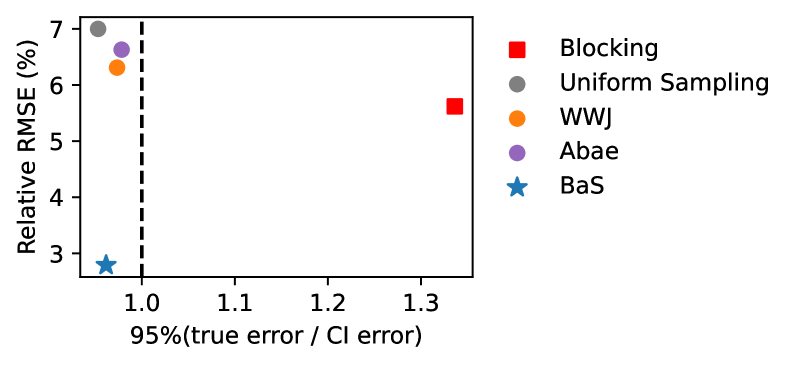
Analytical join queries over unstructured data are increasingly prevalent in data analytics. Applying machine learning (ML) models to label every pair in the cross product of tables can achieve state-of-the-art accuracy, but the cost of pairwise execution of ML models is prohibitive. Existing algorithms, such as embedding-based blocking and sampling, aim to reduce this cost. However, they either fail to provide statistical guarantees (leading to errors up to 79% higher than expected) or become as inefficient as uniform sampling.

We propose blocking-augmented sampling (BaS), which simultaneously achieves statistical guarantees and high efficiency. BaS optimally orchestrates embedding-based blocking and sampling to mitigate their respective limitations. Specifically, BaS allocates data tuples in the cross product into two regimes based on the failure modes of embeddings. In the regime of false negatives, BaS uses sampling to estimate the result. In the regime of false positives, BaS applies embedding-based blocking to improve efficiency. To minimize the estimation error given a budget for ML executions, we design a novel two-stage algorithm that adaptively allocates the budget between blocking and sampling. Theoretically, we prove that BaS asymptotically outperforms or matches standalone sampling. On real-world datasets across different modalities, we show that BaS provides valid confidence intervals and reduces estimation errors by up to 19$\times$, compared to state-of-the-art baselines.

1. Introduction

The increasing capability of machine learning (ML) and large language models (LLMs) allows data analysts to analyze semantically related objects across multiple unstructured datasets automatically (Nogueira and Cho, 2019; Reimers and Gurevych, 2019; Khattab and Zaharia, 2020; Liu et al., 2016, 2017; Zhou et al., 2019; He et al., 2021; Li et al., 2022; Radford et al., 2021). For example, a business investor can analyze differences in stock prices among related companies (Zhang et al., 2021) by computing the AVG over a join of two sets of company records with a join condition based on the company description.

⬇

SELECT AVG(c1.price - c2.price) FROM companies AS c1

JOIN companies AS c2 ON NL(‘Company: {c1.description} and Company: {c2.description} build similar products’)’

To accurately process queries whose join conditions involve arbitrary semantics, an analyst can manually label or apply an ML model to each pair of records. This pairwise evaluation method has demonstrated high accuracy across various applications, including small language models for entity matching (Li et al., 2020b; Paganelli et al., 2022; Teong et al., 2020) and text retrieval (Khattab and Zaharia, 2020; Nogueira and Cho, 2019; Reimers and Gurevych, 2019; Zhuang et al., 2023), vision-language models for image-text retrieval (Li et al., 2022; Vendrow et al., 2025; Li et al., 2021a), and large language models for challenging data wrangling tasks (Narayan et al., 2022; Peeters et al., 2025; Wang et al., 2025; Patel et al., 2025; Liu et al., 2024). We refer to this pairwise evaluation method as the Oracle. Unfortunately, the Oracle method can be prohibitively expensive since the number of ML model invocations grows at least quadratically with the number of data records and exponentially with the number of tables to be joined.

To mitigate these high costs, researchers have proposed two approximation methods that reduce the number of ML model invocations: embedding-based blocking and sampling. However, when used to process analytical join queries over unstructured data, embedding-based blocking can lead to arbitrary errors, while sampling is inefficient.

Embedding-based Blocking. In efficient entity matching systems, embedding-based blocking first uses embedding similarities to filter out data pairs and then applies ML models for pairwise evaluation (Thirumuruganathan et al., 2021; Mudgal et al., 2018; Li et al., 2020b, 2021b). In contrast to the Oracle method that applies ML models to each data pair, embedding-based blocking applies embedding models on each data record and only uses the Oracle on a limited number of data pairs, which effectively reduces the cost of executing expensive ML models.

However, embedding models can be unreliable and are not guaranteed to precisely capture the semantics of interest (Muennighoff et al., 2023; Thakur et al., ; Huang et al., 2023; Li et al., 2023a). Consequently, two data records that satisfy the join condition may have a low embedding similarity (i.e., false negatives), causing embedding-based blocking to filter out such a pair of records. In this case, when used to compute data aggregations, embedding-based blocking skews aggregation results toward data with high embedding similarity. Thus, embedding-based blocking does not provide statistical guarantees. Empirically, we find that blocking can result in errors up to 79% higher than expected even when the threshold of filtering is calibrated on a validation dataset (§7.2).

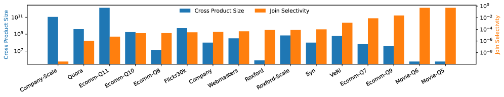
Sampling. To achieve statistical guarantees, researchers have used sampling techniques to process analytical join queries with approximate semantics (Acharya et al., 1999; Vengerov et al., 2015; Haas and Hellerstein, 1999). With independently and identically distributed samples, we can calculate confidence intervals (CIs) to provide statistical guarantees. However, due to the sparsity of positive pairs (Figure 4, §7.1), uniform sampling can be inefficient, requiring a large sample size to achieve a small error. In Section 7.3, we show that achieving an average error of 5% for the Company dataset requires uniformly sampling $1.4\times 10^{7}$ data pairs and processing them with the Oracle (Figure 7(a)).

We propose Weighted Wander Join (WWJ) to improve the efficiency of sampling using embeddings. WWJ extends Wander Join (Li et al., 2016), an efficient join algorithm for structured data, with an approximate index computed from embeddings. Intuitively, WWJ follows the idea of importance sampling to reduce sampling variance by upweighting the probability of sampling data pairs with high embedding similarities (Kloek and Van Dijk, 1978). Nevertheless, the effectiveness of WWJ depends heavily on the precision of the embeddings. We empirically show that WWJ becomes as inefficient as uniform sampling, if the embedding similarities contain many false positives (Figure 7, §7.3).

Blocking-augmented Sampling (BaS). To address the limitations of standard statistical methods over imperfect embeddings, we propose Blocking-augmented Sampling. Our core novelty lies in the dynamic orchestration of two techniques based on the specific failure modes of embedding models: false negatives (which break blocking) and false positives (which break importance sampling).

BaS addresses this by treating the blocking threshold not as a static filter, but as a dynamic decision boundary that splits the search space into two regimes: (1) a blocking regime (high similarity, high false positive risk), where we deterministic execute the Oracle to eliminate variance caused by frequent non-matches; (2) a sampling regime (low similarity, high false negative risk), where we apply importance sampling to correct the bias introduced by blocking. Unlike standard stratified sampling where strata are fixed, BaS solves a complex optimization problem to determine the optimal boundary between these regimes.

Given a fixed budget for Oracle executions, it is challenging to optimally allocate the data pairs into two regimes and assign the budget between blocking and WWJ. Empirically, the optimal allocation that minimizes the estimation error varies significantly across different datasets. Using the optimal allocation can result in estimation errors that are up to 99% smaller than the worst allocation (Figure 10, §7.5). Theoretically, we show that the optimal budget allocation depends on the sampling variance of WWJ on different parts of the dataset. Unfortunately, the sampling variance is unknown unless the Oracle is executed on the entire dataset.

To automatically determine the optimal allocation, we propose an adaptive allocation algorithm via two-stage stratified sampling. Initially, BaS stratifies data tuples based on the embedding similarity. In the first stage, BaS applies pilot sampling (Kish, 2011) to estimate the sampling variance of each stratum. Based on these estimates, BaS determines the optimal allocation that minimizes the overall estimated sampling variance. In the second stage, BaS executes WWJ and blocking according to the allocated regime and budget. We prove that BaS not only converges to the optimal budget allocation but also outperforms or matches standalone WWJ asymptotically. Finally, to obtain valid CIs as statistical guarantees, BaS adopts bootstrapping that estimates statistical distributions via resampling (Hall, 1988; Pol and Jermaine, 2005). We theoretically justify the validity and empirically demonstrate the coverage of the derived CIs.

We implement WWJ and BaS in a prototype system called JoinML to accelerate approximate analytical join queries over unstructured data. We evaluate JoinML using six real-world datasets and two synthetic datasets, including text, image, and bimodal data. Our results reveal that BaS reduces the root mean squared error by up to 19$\times$ compared to the uniform sampling, blocking and prior systems for semantic operators. We also show that the CIs provided by BaS achieve the expected coverage. In additional to analytical queries, we show that BaS can improve the precision of selection queries over unstructured data by up to 69%, compared to baselines. In our ablation study, we show that the allocation algorithm closely approaches optimal performance. Our contributions are as follows:

1. We develop JoinML algorithms, WWJ and BaS, that can accurately and efficiently answer approximate analytical join queries with statistical guarantees.

2. We prove the convergence rate of BaS to the optimal allocation and that BaS outperforms or matches standalone sampling asymptotically.

3. We implement and evaluate JoinML in real-world text, images, and bimodal datasets, reducing root mean squared errors by up to 19$\times$ compared to state-of-the-art baselines.

2. Query Syntax and Semantics

⬇

SELECT {AVG | SUM | COUNT} {field | EXPR(field)}

FROM table_name1 JOIN table_name2 JOIN ...

ON NL(join_condition) AND ...

ORACLE BUDGET b WITH PROBABILITY p

Figure 1. Query syntax of JoinML.

JoinML accelerates analytical queries involving joins and similarity-based join conditions. Currently, we support linear aggregates, including COUNT, SUM, and AVG. We illustrate the query syntax in Figure 1. Besides a SQL query, users can specify an execution budget of Oracle and the coverage probability for the CI. To understand the semantics of a JoinML query, we introduce the concepts of Oracle and embedding similarity.

Oracle. We define Oracle as a method that operates on a pair of records to determine if they satisfy the join condition. We assume that the Oracle is the state-of-the-art method that outputs the ground-truth label. For example, the Oracle method can be a foundation model that decides if two sentences contain the same entity (Narayan et al., 2022), a fine-tuned model that accesses whether two images show the same car (Liu et al., 2016, 2017), or a human labeler for particularly challenging tasks (Ziems et al., 2024; Demszky et al., 2020; Pilehvar and Camacho-Collados, 2018).

Embedding Similarity. We define the similarity between two records $t_{1}$ and $t_{2}$ as the cosine similarity of their embedding vectors:

$$\mathrm{sim}\left(E(t_{1}),E(t_{2})\right)=\frac{E(t_{1})^{\top}\cdot E(t_{2})}{|E(t_{1})|\cdot|E(t_{2})|}$$

The embedding vectors $E(\cdot)$ can be obtained by applying a pre-trained embedding model on each data record individually. Therefore, compared to Oracle methods that are executed on each pair of records, using embedding similarity incurs significantly lower computational costs. However, since the embedding model does not consider the joint semantic across data records, the embedding similarity can be less accurate than the Oracle.

Query Semantics. A JoinML query will output an estimate $\hat{\mu}$ of the answer and a CI $[l,u]$. Suppose $\mu$ is the result of processing the query exhaustively via the Oracle. With a budget $b$ and a probability $p$, we provide the following guarantees: (1) The Oracle will not be executed on more than $b$ pairs; (2) $\mathbb{P}\left[l\leq\mu\leq u\right]\geq p$. Our query semantics and guarantees are similar to prior AQP over unstructured data without joins (Kang et al., 2019, 2020, 2021).

3. Use Cases

Analytical queries with joins are increasingly prevalent in analytics over unstructured data, such as plagiarism analysis (Foltỳnek et al., 2019; Barrón-Cedeño et al., 2013; Shoyukhi et al., 2023), business analysis (Zhang et al., 2021; Lei et al., 2024), and traffic condition monitoring (Coifman, 1998; Zapletal and Herout, 2016). In addition to the business analysis query introduced in Section 1, we demonstrate two more typical use cases. In the example queries, we can use an oracle budget of 1,000,000 and a confidence of 0.95.

Plagiarism Analysis. Sentence-level analysis is a common approach in plagiarism detection that involves comparing each sentence of an input article with every sentence in a reference collection (Foltỳnek et al., 2019; White and Joy, 2004). The plagiarism score of the article can be calculated as the percentage of sentences that are paraphrased from the reference collection. To compute the percentage, we need to join the sentences of the article with those in the reference collection and count the number of sentence pairs that are considered paraphrased:

⬇

SELECT COUNT(*) FROM article JOIN db ON NL(‘{article.sentence} is paraphrased from {db.sentence}.’)’

Traffic Analysis. An urban planner may be interested in analyzing the average traffic time across a road segment by calculating the time for the same vehicle to travel from one end to the other (Coifman, 1998). To find the time difference, the urban planner needs to join two videos and identify common vehicles:

⬇

SELECT AVG(video1.ts - video2.ts) FROM video1 JOIN video2 ON NL(‘Frame {video1.frame} and Frame {video2.frame} contains the same car.’)’

Join Order Optimization. Optimizing multi-way semantic joins requires accurate cardinality estimates to determine efficient execution orders. However, for unstructured predicates requiring ML evaluation, deriving these statistics is prohibitively expensive. BaS resolves this by efficiently estimating COUNT with tight confidence intervals using a minimal budget. These estimates allow the query optimizer to reliably select the optimal join order, preventing performance regressions caused by poor planning without requiring full pairwise evaluation (Section 7.4).

4. Background

Existing algorithms in approximate query processing (AQP) and entity matching (EM) can be applied to accelerate analytical join queries over unstructured data. In this section, we introduce two typical algorithms: sampling and blocking.

Figure 2. Given a COUNT query with an Oracle budget of 5,000,000 and a probability of 95%, sampling algorithms leads to high estimation error while blocking fails to achieve statistical guarantees. Achieving statistical guarantees means that the 95th percentile of the true error is less than the error bounded by a 95% CI (to the left of the dashed line).

4.1. Sampling

Sampling techniques are widely used in AQP to reduce query costs while providing CIs as statistical guarantees. Prior work has developed efficient sampling algorithms for analytical join queries with join keys, such as correlated sampling (Vengerov et al., 2015), universe sampling (Huang et al., 2019), and Wander Join (Li et al., 2016). We can apply these algorithms to accelerate joins over unstructured data.

Limitations. Existing efficient sampling algorithms for joins over structured data requires exact indices or hash functions on the join keys. However, there is no join key for semantic join queries over unstructured data. To obtain semantic indices or hash functions, one way is applying the Oracle method across all data tuples, which is prohibitively expensive. Without indices or hash functions, we can only use uniform sampling, which is inefficient because positive pairs are often sparse in the cross product of tables. Empirically, given a fixed error budget, uniform sampling can lead to 2.6$\times$ higher error than our proposed method (Figure 2).

1

2

Input : input tables $T_{1},T_{2}$, Oracle $O(\cdot)$, embedding $E(\cdot)$, attribute $g(\cdot)$, embedding similarity $\mathrm{sim}(\cdot,\cdot)$, similarity score threshold $\tau$

3

4$S\leftarrow\emptyset$

5 for each data record $t_{1}$ in $T_{1}$ do

6    for each data record $t_{2}$ in $T_{2}$ do

7       $\tau_{i}=\mathrm{sim}\left(E(t_{1}),E(t_{2})\right)$

8      

9   if $\tau_{i}\geq\tau$ then

       $S\leftarrow S\cup\{(t_{1},t_{2})\}$ // Forming data blocks

10      

11   

12$X\leftarrow\{O(s)\cdot g(s):s\in S\}$

13 return $\sum_{i=1}^{|X|}X_{i}$

14

15

Algorithm 1 Emedding-based blocking for a SUM aggregation over a join of two tables.

4.2. Embedding-based Blocking

To reduce the number of pairwise comparisons, traditional blocking algorithms typically uses a blocking phase to prune the search space (Papadakis et al., 2020; Li et al., 2020a; Christophides et al., 2015; Fellegi and Sunter, 1969; Papadakis et al., 2015; Draisbach and Naumann, 2011; Bilenko et al., 2006; Michelson and Knoblock, 2006; Papadakis et al., 2012). While traditional blocking algorithms cluster records into disjoint buckets (blocks), modern deep learning approaches use embedding-based blocking (Papadakis et al., 2020; Thirumuruganathan et al., 2021; Mudgal et al., 2018; Li et al., 2020b). Throughout this paper, blocking refers to this embedding-based filtering with thresholds. It implicitly defines a block of candidate pairs as the set of tuples whose embedding similarities exceed a threshold $\tau$. By filtering out pairs below $\tau$ (Line 5 in Alg. 1 and 2), the algorithm effectively blocks unrelated data from expensive pairwise comparison. We show the procedure for estimating SUM in Alg. 1, where the Oracle is executed only on the candidate block.

In practice, we often have a budget for Oracle invocations and may need to join more than two tables. To address these, we present a direct extension of the original embedding-based blocking as a baseline in Algorithm 2. As shown, to satisfy the predefined Oracle budget, we perform random sampling over the resulting set of data tuples after filtering and then estimate the target statistic using the sample. We obtain a point estimate and a CI via a standard approach. Furthermore, to support $k$-table joins ($k\geq 2$) in general, we calculate the similarity of a $k$-tuple as the joint probability that the $k$ tuples match, assuming embedding similarity approximates the probability that two data records match.

Limitations. Unfortunately, the predefined threshold $\tau$ does not guarantee zero false negatives on the evaluation dataset, even when we calibrate it on a validation dataset. Therefore, there is no guarantee on the error of the point estimate or the validity of the CI. Empirically, we show that blocking can result in true errors higher than the errors bounded by the provided CIs (Figure 2).

1

Input : input tables $T_{1},\ldots,T_{k}$, Oracle $O(\cdot)$, embedding $E(\cdot)$, attribute $g(\cdot)$, embedding similarity $\mathrm{sim}(\cdot,\cdot)$, similarity score threshold $\tau$, oracle budget $b$, probability $p$

2

3$D\leftarrow\mathrm{CrossProduct}(T_{1},\ldots,T_{k})$

4 $S\leftarrow\emptyset$

5 for each $k$-tuple $\left(t_{1},\ldots,t_{k}\right)$ in $D$ do

6    $\tau_{i}\leftarrow\prod_{j=1}^{k-1}\mathrm{sim}\left(E(t_{j}),E(t_{j+1})\right)$

7    if $\tau_{i}\geq\tau$ then

       $S\leftarrow S\cup\{\left(t_{1},\ldots,t_{k}\right)\}$ // Forming data blocks

8      

9   

10if $|S|\leq b$ then

11    $X\leftarrow\{O(s)\cdot g(s):s\in S\}$

12    return $\sum_{i=1}^{|X|}X_{i}$

13   

14else

15    $\tilde{S}\leftarrow\textnormal{\text{Sample}}(S,b)$

16    $X\leftarrow\{O(s)\cdot g(s):s\in\tilde{S}\}$

17    return StandardCI($X,p,|S|$)

18Function StandardCI($X,p,N$):

19    $\hat{\mu}\leftarrow\frac{1}{|X|}\sum_{i=1}^{|X|}X_{i}$

20    $\hat{\sigma}\leftarrow\frac{1}{|X|-1}\sum_{i=1}^{|X|}\left(X_{i}-\hat{\mu}\right)^{2}$

21    $l,u\leftarrow\hat{\mu}\mp z_{(1+p)/2}\cdot\frac{\hat{\sigma}}{\sqrt{|X|}}$

22    return $N\hat{\mu},Nl,Nu$

23   

24

Algorithm 2 Embedding-based blocking for SUM with a predefined Oracle budget.

5. Efficient JoinML Algorithms with Guarantees

In this section, we present our novel JoinML algorithms for analytical join queries over unstructured data which overcomes the limitations of baselines, simutaneously achieving statistical guarantees and high efficiency. Our key insights are:

1. The sparsity of positive tuples in the cross product of tables makes uniform sampling inefficient. To address it, we design a non-uniform sampling algorithm (i.e., Weighted Wander Join) with the embedding as the approximate index (§5.1).

2. False positives of the embedding similarity compromise the efficiency of WWJ. Therefore, we augment WWJ with embedding-based blocking (§5.2) and adaptive data allocation (§5.3).

Finally, we extend our algorithms to handle selection join queries with joins with recall guarantees (§5.4).

5.1. Weighted Wander Join

Figure 3. Illustration of Wander Join with indices, without indices, and with approximate indices. Black dots are data records while solid connections are viable paths during random walks. The widths of edges in (c) show the probability of choosing paths.

As we discussed in Section 4.1, existing sampling algorithms for join queries often fall back to inefficient uniform sampling due to the difficulty and prohibitive costs of obtaining exact semantic indices or hash functions for unstructured data. For example, Wander Join, one of the state-of-the-art join algorithm for structured data, formulates join operations into random walks over the records of different join tables (Li et al., 2016). For each iteration of the Wander Join, we randomly walk to a record that satisfies the join conditions (Figure 3a). Knowing which records can satisfy the join condition requires indices over the join columns. Without such indices, Wander Join would simply randomly choose any record in each iteration, which is equivalent to uniform sampling (Figure 3b).

While exact semantic indices is expensive to compute for unstructured data, we can use embeddings to construct approximate indices and extend Wander Join accordingly. Specifically, in each iteration, instead of randomly sampling a record satisfying join conditions, we sample a record with a probability proportional to the embedding similarity (Figure 3c). We refer to this algorithm as the Weighted Wander Join (WWJ) and illustrate the procedure for a SUM aggregate in Algorithm 3.

1

Input : input tables $T_{1},\ldots,T_{k}$, embedding $E(\cdot)$, attribute function $g(\cdot)$, embedding similarity $\mathrm{sim}(\cdot,\cdot)$, oracle budget $b$, probability $p$

2

3$S\leftarrow\emptyset$

4 for $i$ in $1,\ldots,b$ do

5    $t_{i,1}\leftarrow\textnormal{\text{Sample}}(T_{1},1)$

6    for $j$ in $2,\ldots,k$ do

7       $W_{i,j}\leftarrow\{\mathrm{sim}\left(E(t_{i,j-1}),E(t)\right):t\in T_{j}\}$

8       $t_{i,j}\leftarrow\textnormal{\text{WeightedSample}}(T_{j},1,W_{i,j})$

9      

10   $S\leftarrow S\cup\{(t_{i,1},\ldots,t_{i,k})\}$

11    $W(s)\leftarrow\frac{1}{|T_{1}|}\prod_{j=2}^{k}\mathrm{sim}\left(E(t_{i,j-1}),E(t_{i,j})\right)$

12$X\leftarrow\left\{O(s)\cdot g(s)\cdot W(s)^{-1}:s\in S\right\}$

13 return StandardCI($X,p,\prod_{i=1}^{k}|T_{i}|$)

Algorithm 3 Weighted Wander Join algorithm (SUM).

Connection to Importance Sampling. We find that WWJ is an instantiation of importance sampling (Kloek and Van Dijk, 1978). To understand why, we consider a general case of $k$ join tables: $T_{1},\ldots,T_{k}$. WWJ is equivalent to importance sampling with the sampling space being the set of all tuples in the cross product of $T_{1},\ldots,T_{k}$. Each tuple in the sampling space corresponds to a complete walk from $T_{1}$ to $T_{k}$. Given a join order, the sampling weight of each tuple is the multiplication of embedding similarity of pairs:

$$W(t_{1},\ldots,t_{k})=\frac{1}{|T_{1}|}\cdot\prod_{i=2}^{k}\mathrm{sim}\left(E\left(t_{i-1}\right),E\left(t_{i}\right)\right)$$

where we normalize the weight by the size of $T_{1}$ since $T_{1}$ is sampled uniformly. Based on the statistical equivalence between WWJ and importance sampling, we can obtain unbiased estimates and valid CIs in a standard way (Kloek and Van Dijk, 1978), as shown in Algorithm 3, Lines 9-10.

While WWJ requires computing embedding similarities at each step without pre-built index exists, it is more efficient than importance sampling. Naive sampling requires enumerating the cross-product, resulting in exponential complexity $\mathcal{O}(\prod_{i=2}^{k}|T_{i}|)$. In contrast, WWJ decomposes the problem into sequential steps. In each iteration, we only compute similarities between the current tuple and the $N$ tuples of the next table. Consequently, for a budget $b$, the complexity scales as $\mathcal{O}(b\cdot\sum_{i=1}^{k}|T_{i}|)$. This cost is linear (or quadratic depending on $b$) with respect to table sizes, but crucially avoids the exponential explosion of the cross-product.

Limitations. The statistical efficiency of WWJ depends on the precision of the embedding similarity. When the tuples with high similarity scores all satisfy the join conditions, WWJ converges to Wander Join with exact indices, achieving the best efficiency. However, when there are many false positives (i.e., tuples with high similarity scores violets join conditions), WWJ can repetitively sample negative pairs, leading to an efficiency comparable or even worse than uniform sampling. We empirically show such limitation of WWJ in Section 7.

We find that false positives are often unavoidable, particularly when the pre-trained embedding fails to accurately capture the semantics of the join condition. For example, a pre-trained embedding for text data can capture the semantic characteristic. However, two records that appear semantically similar might not satisfy the join condition that requires two companies to build the same product. In Section 7.6, we show that such issues persist even in state-of-the-art embeddings (Lee et al., 2024; DunZhang, 2024; Li et al., 2023b; Xiao et al., 2023; Rui* et al., 2024).

5.2. Blocking-augmented Sampling

To improve the efficiency of WWJ when there are many false positives, we propose Blocking-augmented Sampling (BaS), which augments WWJ with the blocking algorithm. Specifically, we separate the sampling space into two regimes:

1. The sampling regime ($D_{s}$), characterized by many false negatives, where we apply WWJ.

2. The blocking regime ($D_{b}$), characterized by many false positives, where we directly execute the Oracle.

Intuition. BaS mitigates the limitation of both WWJ and blocking. First, BaS directly applies the Oracle on the blocking regime to mitigate the high sampling variance due to repetitively sampling false positives. Second, BaS can provide statistical guarantees since WWJ does not ignore false negatives. To execute WWJ only on the sampling regime, we can simply set the sampling probability of tuples in the blocking regime to zero. Finally, we combine the results of both regimes to obtain a final estimate of the aggregate.

Formal Description. We describe the estimation procedure formally. Suppose we have an Oracle budget $b$ and a separation of the entire sampling space $D=D_{s}\cup D_{b}$. Then, we execute WWJ on $D_{b}$ with a sample size of $b-|D_{b}|$ and execute the Oracle on $D_{s}$. Finally, we can estimate the aggregate over $D$ by combining the estimate of the aggregate over $D_{s}$ and the true value of the aggregate over $D_{b}$:

(1) $$\widehat{\texttt{COUNT}}=\widehat{\texttt{COUNT}}_{s}+\texttt{COUNT}_{b},\quad\widehat{\texttt{SUM}}=\widehat{\texttt{SUM}}_{s}+\texttt{SUM}_{b}$$

(2) $$\widehat{\texttt{AVG}}=\left(\widehat{\texttt{SUM}}_{s}+\texttt{SUM}_{b}\right)\Big/\left(\widehat{\texttt{COUNT}}_{s}+\texttt{COUNT}_{b}\right)$$

We observe that the combined estimators for COUNT and SUM are unbiased since the estimators over $D_{s}$ is linear. However, the combined estimator for AVG is a ratio estimator, which is asymptotically unbiased at the order of $\mathcal{O}(1/b)$ as proved in the Section 6.8 of (Cochran, 1977). To reduce the bias to the order of $\mathcal{O}(1/b^{2})$, we apply the bias correction based on the Taylor expansion (Cochran, 1977) to our AVG estimator:

(3) $$\widehat{\texttt{AVG}}_{2}=\widehat{\texttt{AVG}}\cdot\left(1-\frac{1}{b-|D_{b}|}\frac{Var\left[\widehat{\texttt{COUNT}}\right]}{\widehat{\texttt{COUNT}}^{2}}\right)$$

Challenges. To realize the advantages of BaS over WWJ and blocking, we need to tackle two challenges. First, we need to find an optimal separation such that the estimation error is minimized given an Oracle budget. Second, we need to obtain valid CIs for our combined estimators, achieving the specified coverage probability $p$. We introduce our adaptive allocation algorithms to address them.

5.3. BaS with Adaptive Allocation

Given an Oracle budget $b$, an optimal allocation should minimize the mean squared error (MSE) of the aggregate estimate. In this allocation optimization problem, we need to decide whether a tuple in the sampling space $D$ should be allocated to the sampling regime or the blocking regime. Unfortunately, tuple-level allocation can be prohibitively expensive due to the size of the sampling space. To address it, we formulate the optimization problem into a stratum-level allocation problem, where we first stratify $D$ into a set of strata based on the similarity scores of tuples. In this case, our allocation algorithm determines which strata should be allocated to the blocking regime to minimize the overall MSE in four steps: stratification, adaptive allocation, sampling or blocking execution, and resampling. We explain the entire procedure using a SUM aggregate.

Stratification. Initially, we divide $D$ into a maximum blocking regime and a minimum sampling regime ($D_{0}$). The maximum blocking regime contains tuples with the top $b_{2}=\alpha\cdot b$ similarity scores, where $\alpha$ is a parameter between 0 and 1 to control the size of the maximum blocking regime. Based on $\alpha$, we reserve $b_{2}$ for potential blocking and the remaining budget $b_{1}=b-b_{2}$ for adaptive allocation. Next, we stratify the maximum blocking regime into $K$ strata ($D_{1},\ldots,D_{K}$) with equal sizes (Alg. 4, Lines 1-5). Following prior work about stratified sampling for approximate query processing (Kang et al., 2021), BaS automatically determines the number of strata $K$ to ensure that each stratum has an Oracle budget of at least 1,000.

With the stratification, we formulate the allocation optimization problem. Given the stratified sampling space $D_{0},\ldots,D_{K}$, an aggregate AGG, similarity scores $W$, and an Oracle budget $b$, our target is to find an optimal allocation $\beta$ that minimizes the MSE of the estimated AGG. The allocation $\beta$ specifies a subset of the maximum blocking regime ($D_{1}\ldots,D_{K}$) that will directly execute the Oracle while the rest of strata will execute WWJ. We formulate this optimization problem as follows:

(4) $$\beta^{*}=\mathop{\arg\min}_{\beta\subset\{1,\ldots,K\}}MSE_{\texttt{AGG}}(D,\beta,W,b)$$

Input : input tables $T_{1},\ldots,T_{k}$, similarity score $W(\cdot)$, attribute $g(\cdot)$, number of stratum $K$, maximum blocking ratio $\alpha$, oracle budgets $b_{1}$ and $b_{2}$, probability $p$

1

/* Stratification */

2 $D^{\prime}\leftarrow\textnormal{\text{Top}}(\textnormal{\text{CrossProduct}}(T_{1},\ldots,T_{k}),W,\alpha(b_{1}+b_{2}))$

3 $D^{\prime}\leftarrow\textnormal{\text{SortDesc}}(D^{\prime},W)$

4 $D_{0}\leftarrow D\backslash D^{\prime}$

5 for $i$ in $1,\ldots,K$ do

6    $D_{i}\leftarrow D^{\prime}\left[\alpha(i-1)(b_{1}+b_{2})/K:\alpha\cdot i(b_{1}+b_{2})/K\right]$

/* Adaptive Allocation via Pilot Sampling */

7 for $i$ in $0,\ldots,K$ do

8    $n^{(1)}_{i}\leftarrow\frac{\sum_{x\in D_{i}}W(x)}{\sum_{x\in D}W(x)}b_{1}$

9    $S^{(1)}_{i}\leftarrow\textnormal{\text{WeightedSample}}(D_{i},n_{i},W)$

10    $X_{i}^{(1)}\leftarrow\left\{g(s)\cdot O(s)\cdot W(s)^{-1}:s\in S^{(1)}_{i}\right\}$

11    $\hat{\sigma}_{i}^{2}\leftarrow|D_{i}|^{2}\cdot Var\left[X_{i}^{(1)}\right]$

12   

13$\beta^{*}\leftarrow\mathop{\arg\min}_{\beta}\ \sum_{\begin{subarray}{c}i\notin\beta\end{subarray}}\hat{\sigma}_{i}^{2}\bigl/\textnormal{\text{BudgetAssign}}(b_{2},W,\beta,i,D)$

/* Sampling + Blocking */

14 for $i\notin\beta^{*}$ do

15    $n^{(2)}_{i}\leftarrow\textnormal{\text{BudgetAssign}}(b_{2},W,\beta^{*},i,D)$

16    $S^{(2)}_{i}\leftarrow\textnormal{\text{WeightedSample}}(D_{i},n_{i},W)$

17    $X_{i}^{(2)}\leftarrow\left\{g(s)\cdot O(s)\cdot W(s)^{-1}:s\in S^{(2)}_{i}\right\}$

18   

19for $i\in\beta^{*}$ do

20    $S^{(2)}_{i}\leftarrow\textnormal{\text{Sample}}(D_{i},|D_{i}|)$

21    $X_{i}^{(2)}\leftarrow\left\{g(s)\cdot O(s):s\in S_{i}^{(2)}\right\}$

22   

/* CI via Resampling */

23 $X\leftarrow X^{(1)}\cup X^{(2)}$

24 return $\textnormal{\text{ResamplingCI}}(X,p,D)$

25Function BudgetAssign($b,W,\beta,i,D$):

26    return $\left(b-\sum_{j\in\beta}|D_{j}|\right)\frac{\sum_{s\in D_{i}}W(s)}{\sum_{j\notin\beta}\sum_{s\in D_{j}}W(s)})$

27   

28

Algorithm 4 BaS with Adaptive Allocation for a SUM Aggregate

Adaptive Allocation via Pilot Sampling. To address the optimization problem, we first calculate the MSE given an allocation $\beta$. We observe that our estimator of the SUM aggregate (Equation 1) is unbiased. Therefore, we can calculate overall MSE as the summation of sampling variance of each stratum in the sampling regime:

(5) $$MSE_{\texttt{SUM}}=\sum_{\begin{subarray}{c}0\leq i\leq k,i\notin\beta\end{subarray}}Var\left[\frac{|D_{i}|}{n_{i}}\sum_{s\in S_{i}}\frac{O(s)g(s)}{W(s)}\right]$$

where $S_{i}$ is the sampled tuple of $D_{i}$ following the procedure of WWJ and $n_{i}$ is the (hypothetical) Oracle budget assigned to stratum $D_{i}$. For a stratum in the blocking regime, $n_{i}=|D_{i}|$. For a stratum in the sampling regime, we follow the scheme of importance sampling and assign the budget proportional to the sum of similarity scores:

$$n_{i}=\frac{(b-\sum_{j\in\beta}|D_{i}|)\cdot\sum_{s\in D_{i}}W(s)}{\sum_{1\leq j\leq K,j\notin\beta}\sum_{s\in D_{j}}W(s)}$$

Unfortunately, the sampling variance in Equation (5) is unknown unless we apply the Oracle to the entire sampling regime. To address this, we apply pilot sampling, a sampling procedure that is used to obtain statistics to guide the main sampling later. In our algorithm, we use pilot sampling to estimate the sampling variance with an Oracle budget of $b_{1}$ (Algorithm 4, Line 8). Then, we can estimate the optimal allocation using the estimated variance (Algorithm 4, Line 11). In Section 6, we show that our estimated optimal allocation converges to the optimal allocation at the rate of $\mathcal{O}(1/\sqrt{b_{1}})$. To avoid applying Oracle on the same data tuples twice, we cache the Oracle results obtained in the pilot sampling stage for next stages.

Sampling+Blocking. Given the optimal allocation $\beta^{*}$, we use the remaining Oracle budget $b_{2}$ to execute WWJ on strata that are allocated to the sampling regime and execute the Oracle on the strata that are allocated to the blocking regime. We merge the results of using the budget $b_{1}$ (for pilot sampling) and the budget $b_{2}$ to estimate the aggregate (Alg. 4, Lines 12-18.)

CI via Resampling. As we merge the sample from two dependent stages, the resulting sample is not independently and identically distributed (i.i.d.). This means we cannot calculate CIs using the Central Limit Theorem (CLT) that assumes i.i.d. data. Applying standard CLT on non-i.i.d. data naively can lead to CIs without valid coverage; for example, a 95% CI might cover the true value with a probability lower than 95%. To guarantee valid coverages, we use resampling for CIs.

We apply the bootstrap-t resampling scheme to calculate CIs with coverage guarantees (Hall, 1988). Given an existing sample $X$, a confidence $p$, bootstrap-t resampling works as follows:

1. Calculate the estimated aggregate $\hat{\mu}$ and its variance $\hat{\sigma}^{2}$.

2. Sample $|X|$ data from $X$ with replacement, resulting in a resample $R_{i}$

3. Calculate the estimation $\hat{\mu}_{i}$ and the variance $\hat{\sigma}_{i}^{2}$ using $R_{i}$.

4. Calculate the t-statistic: $t_{i}=\frac{\hat{\mu}_{i}-\hat{\mu}}{\hat{\sigma}_{i}}$

5. Repeat (2)-(4) for a sufficient number of times. Following prior work (Kang et al., 2021), we use 1,000 resamples.

6. Calculate the $\frac{1-p}{2}$ and $1-\frac{1-p}{2}$ percentile of t-statistics, resulting in $t_{l}$ and $t_{r}$, respectively.

7. Return the CI as: $[\hat{\mu}-t_{l}\hat{\sigma},\hat{\mu}-t_{r}\hat{\sigma}]$

Intuitively, bootstrap-t resampling estimates the CI by measuring the empirical CI when sampling from the empirical distribution of observed data. It further uses t-statistics to adjust the skewness and thus achieves the coverage guarantee at the order of $\mathcal{O}(1/b^{2})$ (Hall, 1988).

We justify this validity by leveraging Theorem 23.9 of (Van der Vaart, 2000), which states that bootstrap CIs are valid if the statistical functional is Hadamard differentiable with respect to the CDF. Since our estimators for SUM and COUNT are linear combinations (and AVG is a ratio of differentiable functionals), they satisfy this condition. We defer the full proof to Appendix B.5.

As shown in Algorithm 4, our resampling step for CI computation operates independent of the adaptive allocation. The allocation objective is to minimize MSE, which inherently optimizes accuracy regardless of whether a CI is requested. Therefore, while skipping CI computation eliminates the resampling overhead, it does not directly improve estimation accuracy. For applications constrained by total latency rather than monetary cost, the computational time saved by omitting resampling could be leveraged to increase the Oracle budget, thereby indirectly improving estimation accuracy.

Handling AVG. We estimate AVG with a ratio estimator (Eq. 2 and 3), which is asymptotically unbiased. Given the independence between SUM and COUNT, we estimate the MSE of AVG as follows:

$$MSE_{\texttt{AVG}}=\frac{1}{n}\left(\frac{\widehat{\texttt{SUM}}}{\widehat{\texttt{COUNT}}}\right)^{2}\left(\frac{MSE_{\texttt{COUNT}}}{\widehat{\texttt{COUNT}}^{2}}+\frac{MSE_{\texttt{SUM}}}{\widehat{\texttt{SUM}}^{2}}\right)$$

where $n=b-\sum_{i\in\beta}|D_{i}|$ is the Oracle budget for the sampling regime. This MSE estimator is based on widely used variance estimator for AVG (Haas and Hellerstein, 1999), which is accurate to the order of $\mathcal{O}(1/b^{2})$ (Cochran, 1977). To handle AVG, we just replace estimators in Algorithm 4.

Handling MIN and MAX. BaS leverages the correlation between embedding similarity and the target attribute. As an example, we estimate MAX by $\widehat{\texttt{MAX}}=\max_{t\in D_{b}\cup S}val(t)$, the maximum observed. Unlike linear aggregates where we minimize global variance, the allocation goal for MAX is to maximize the probability that the true maximum is contained within the blocking regime $D_{b}$. Utilizing the pilot sample, we model the distribution of values in each stratum using Extreme Value Theory (De Haan and Ferreira, 2006) and allocate strata to $D_{b}$ based on their probability of containing values exceeding the current sample maximum. Since the distribution of the sample maximum is non-normal, bootstrap CIs are invalid. Instead, we construct CIs using the observed maximum as a lower bound and the global maximum of the dataset (ignoring join conditions) as an upper bound.

Handling MEDIAN. Estimating the median requires constructing the CDF of the target attribute. BaS estimates the CDF by combining the exact distribution from blocking with the weighted empirical distribution from sampling. Let $F(t)$ be the CDF. We estimate it as:

$$\footnotesize\widehat{F}(t)=\frac{1}{\widehat{N}}\left(\sum_{x\in D_{b}}\mathbb{I}(x\leq t)+\sum_{y\in D_{s}}\frac{1}{\pi_{y}}\mathbb{I}(y\leq t)\right)$$

where $W_{y}$ is the sampling probability. The estimated MEDIAN is then $\widehat{F}^{-1}(0.5)$. The variance of the median estimator depends on the variance of the CDF estimate at the median value. Therefore, our allocation algorithm focuses on minimizing the variance of the CDF in the strata that overlap with the estimated median range derived from the pilot sample. As the median is a statistical functional that is Hadamard differentiable with respect to the CDF, we apply the same bootstrap-t resampling strategy to derive valid CIs.

Handling GroupBy. Group-by queries often suffer from high variance in “tail” groups (groups with low support) under standard sampling, BaS exploits the semantic clustering of embeddings to target specific groups effectively. We first estimate the aggregate for each group $g$. Unlike global aggregation where we minimize total variance, our adaptive allocation for group-by queries minimizes the maximum relative error across all discovered groups. By using pilot samples to estimate the conditional probability of groups within strata, BaS prioritizes blocking in strata containing high densities of “hard-to-estimate” groups. Finally, we use bootstrap-t to provide simultaneous confidence intervals, accounting for the multiple hypothesis testing in multi-group estimation.

Algorithm Complexity. Consider a chain join of $k$ tables with size $N_{1},\ldots,N_{k}$ and $b\ll\prod_{i=1}^{k}N_{i}$. BaS has a time complexity of $\mathcal{O}\left(\prod_{i=1}^{k}N_{i}\right)$ and a space complexity of $\mathcal{O}\left(\sum_{i=1}^{k-1}N_{i}N_{n+1}+b\log b\right)$. This complexity is higher than that of uniform sampling, which has both time and space complexities of $\mathcal{O}(b)$, because BaS incorporates similarity scores. Additionally, BAS has higher complexity than WWJ, which has time and space complexities $\mathcal{O}\left(b\cdot\sum_{i=2}^{k}N_{i}\right)$, primarily due to the stratification. However, when compared to threshold-based blocking, which shares the same time complexity with BaS and has a space complexity of $\mathcal{O}(b)$, BaS only incurs a small overhead to sort the top $\alpha b$ records. Furthermore, BaS is more efficient than Abae, which involves sorting all similarity scores (Kang et al., 2021). Finally, BaS shares the same time complexity with BlazeIt, which applies control variates over the cross product (Kang et al., 2019).

Although BaS has a time complexity that increases exponentially with the number of tables, the leading order of the time complexity is attributed to comparing floating-point numbers using CPUs, which is significantly faster than the Oracle. Our latency profiling reveals that BaS’s CPU computations take up to 90 seconds on our datasets, costing $0.03 on AWS—making it $10^{6}\times$ cheaper than running Oracle with GPT-4o mini.

When the table size or the number of tables is so large that the cross product cannot fit into memory, threshold-based blocking in BaS becomes prohibitively expensive. To mitigate this, we apply the nearest neighbor-based blocking (Christen, 2011). It effectively joins each record of the left table with the top $b^{\prime}$ records of the right table for each join, where $b^{\prime}=\left(\alpha n/N_{1}\right)^{1/(k-1)}$. This method has a time complexity of $\mathcal{O}\left(b\cdot\sum_{i=2}^{k}N_{i}\right)$ and a space complexity of $\mathcal{O}\left(b\right)$, making the complexity of BaS comparable to WWJ and significantly lower than Abae and BlazeIt. We show that BaS with nearest neighbor-based blocking remains more efficient than the baselines (§7.3).

5.4. BaS for Selection Queries

We first review approximate selection queries. Consider a selection query $Q$ that, when executed exactly, outputs a set of records $T$. If $Q$ is processed approximately, the result is $T^{\prime}$. As established in prior work (Kang et al., 2020), we say that $T^{\prime}$ achieves the recall target $\gamma$ and confidence $p$ if $\mathbb{P}[|T\cap T^{\prime}|/|T|\geq\gamma]\geq p$.

To process such queries, prior work calculates a score for each data and outputs all tuples with scores higher than a threshold $\tau_{s}$ (Kang et al., 2020). The score approximately reflects the probability of a tuple satisfying the predicate, while $\tau_{s}$ is estimated using sampling to achieve recall guarantees.

With BaS, we can improve the selection quality by maximize the threshold $\tau_{s}$. This is achieved by adaptive allocating data to minimize the recall target $\gamma_{s}$ for the sampling regime. To formulate the allocation problem, we first translate the overall recall target $\gamma$ to the recall target of the sampling regime $\gamma_{s}$ through the following lemma. We defer the full proof to Appendix B.4.

Lemma 5.1.

With a probability higher than $p$, we can achieve the overall recall target $\gamma$ if $\gamma_{s}$ satisfies

$$\gamma_{s}\geq\gamma-(1-\gamma)\frac{\texttt{COUNT}_{b}}{\mathrm{UB}(\texttt{COUNT}_{s},Var[\texttt{COUNT}_{s}],b,p)}$$

where

$$\mathrm{UB}(\mu,\sigma^{2},b,p)=\mu+\frac{\sigma}{\sqrt{b}}\sqrt{2\log\frac{2}{1-p}}$$

Given a stratification $D_{0},\ldots,D_{K}$ and a budget $b_{2}$, we find the optimal allocation $\beta^{*}$ to minimize $\gamma_{s}$:

$$\beta^{*}=\mathop{\arg\max}_{\beta\subset\{1,\ldots,K\}}\frac{\texttt{COUNT}_{i}}{\sum_{i\notin\beta}\mathrm{UB}(\texttt{COUNT}_{i},Var[\texttt{COUNT}_{i}],b_{i},\frac{p+k-1}{k})}$$

where $\texttt{COUNT}_{i}=\sum_{s\in D_{i}}O(s)$ is the number of matching tuples in stratum $i$ and $b_{i}$ is the assigned budget for stratum $i$. Similar to aggregation queries, we approximately solve the allocation problem with estimated $\texttt{COUNT}_{i}$ and $Var[\texttt{COUNT}_{i}]$ using the pilot sampling.

Handling TopK Heavy Hitters Selection. A heavy-hitter TopK query identifies the $K$ entities with the most appearance (Yi and Zhang, 2009; Cormode et al., 2003; Wang and Tao, 2018). This generalizes the selection problem with a dynamic threshold determined by the $K$-th value. We estimate COUNT for every candidate value using the combined estimator from Equation 1. Let $\widehat{V}_{e}$ be the estimated value for entity $e$. We return the set of $K$ entities with the largest $\widehat{V}_{e}$. To ensure the correctness of the ranking, we minimize the swapping probability between the $K$-th ranked entity and the $(K+1)$-th ranked entity. We adapt our allocation objective to minimize the estimation variance specifically for candidates whose estimates are close to the threshold $\tau$ (the estimated $K$-th value). We provide guarantees on the recall: with probability $p$, the returned set contains the true TopK entities. We achieve this by computing simultaneous confidence intervals for the candidate entities using bootstrap-t, ensuring that the lower bound of the $K$-th item exceeds the upper bound of the $(K+1)$-th item.

5.5. Practical Guidelines

We offer the following deployment guidance. BaS is beneficial when the cost of Oracle significantly outweighs the overhead of embedding similarity calculations. For LLM-based predicates (e.g., GPT-4), Oracle costs are typically orders of magnitude higher than similarity computation, making BaS highly effective. For cold-start scenarios, we recommend allocating 15–30% of the budget to the maximum blocking regime ($b_{2}$) to provide a balanced search space for the optimizer without over-constraining the sampling budget. BaS automatically tunes $K$ to ensure each stratum receives $>1000$ samples. For small budgets, we enforce a minimum $K=5$ to ensure sufficient granularity. Finally, BaS is model-agnostic. For semantic joins (e.g., product descriptions), we recommend dense embeddings (e.g., CLIP (Radford et al., 2021)). For lexical joins, sparse vectors (e.g., TF-IDF) often yield sharper boundaries. To achieve better performance with BaS, we recommend evaluating the false positive and false negative rates of different embeddings on a small data sample.

Figure 4. Cross product size and join selectivity of the 16 evaluated datasets: real-world, SemBench, and synthetic workloads.

6. Theoretical Analysis of BaS

In our analysis, we first show MSE of BaS converges to the MSE with optimal allocation asymptotically at the rate $\mathcal{O}\left(b_{1}^{-1/2}\right)$. Furthermore, we compare the MSE of BaS with that of WWJ, showing that BaS outperforms or matches WWJ asymptotically.

6.1. BaS Converges to the Optimal Allocation

BaS applies pilot sampling to approximately solve the minimization problem in Equation 4. Theorem B.1 shows that the MSE with estimated minimizer $\widehat{\beta}^{*}$ converges to the MSE with the true minimizer $\beta^{*}$ at the rate of $\mathcal{O}\left(1/\sqrt{b_{1}}\right)$.

Theorem 6.1.

The MSE with the estimated minimizer $\hat{\beta}^{*}$ converges to that with the true minimizer $\beta^{*}$ at the rate:

$$\frac{MSE(D,\widehat{\beta}^{*},W,b_{2})-MSE(D,\beta^{*},W,b_{2})}{MSE(D,\beta^{*},W,b_{2})}=\mathcal{O}\left(\frac{1}{\sqrt{b_{1}}}\right)$$

Intuitively, we observe that statistics for allocation determination, specifically the sample mean and sample variance, converge to their true values at a rate proportional to $1/\sqrt{b_{1}}$. Theoretically, we demonstrate the MSE of BaS converges to that of the optimal allocation at the same rate. This is because the arithmetic operations involved in calculating the MSE (i.e., summation, multiplication by constants, and division by constants) do not change the convergence rate. We defer a full proof to Appendix B.2.

6.2. BaS Outperforms or Matches WWJ

Notation. In addition to the notations we introduced in Section 5, We define that $\tilde{D}$ is the set of all positive tuples, the subscript $s$ means the statistic is about the sampling regime of BaS.

We present the comparison of the MSE of BaS and WWJ for the SUM aggregate in Theorem B.2 and defer a full proof to Appendix B.3. We can derive the same result for the COUNT or AVG similarly.

Theorem 6.2.

If there exists an allocation $\beta$ such that the following two conditions hold

(6) $$\mathbb{E}_{s\in\tilde{D}_{s}}\left[\frac{1/|\tilde{D}_{s}|}{W_{s}(s)}\right] \leq\mathbb{E}_{s\in D}\left[\frac{1/|D|}{W(s)}\right]$$

(7) $$\frac{|\tilde{D}_{s}|^{2}}{b_{s}} \leq\frac{|D|^{2}}{b}$$

BaS outperforms WWJ asymptotically, i.e.,

$$MSE^{(\textsc{BaS})}_{\texttt{SUM}}=C\cdot MSE^{(\textsc{WWJ})}_{\texttt{SUM}}+\mathcal{O}\left(b^{-1}b_{1}^{-1/2}\right)$$

where $W_{s}$ is the similarity scores normalized for the sampling regime and $C$ is a coefficient less than 1:

$$C<\frac{|\tilde{D}_{s}|^{2}\big/b_{s}}{|\tilde{D}|^{2}/b}\frac{\mathbb{E}_{s\in\tilde{D}_{s}}\left[\frac{1/|\tilde{D}_{s}|}{W_{s}(s)}\right]}{\mathbb{E}_{s\in\tilde{D}}\left[\frac{1/|\tilde{D}|}{W(s)}\right]}\leq 1$$

Otherwise, BaS matches WWJ asymptotically, i.e.,

$$MSE^{(\textsc{BaS})}_{\texttt{SUM}}\leq MSE^{(\textsc{WWJ})}_{\texttt{SUM}}+\mathcal{O}\left(b^{-1}b_{1}^{-1/2}\right)$$

Theorem 4 suggests two cases when we compare the MSE of BaS and that of WWJ. We discuss both cases in detail.

Case 1: BaS outperforms WWJ asymptotically. Theorem B.2 provides sufficient conditions when JoinML achieves asymptotically better MSE than WWJ. We observe that both conditions can match characteristics of the embedding similarity. First, Condition (6) compares the similarity between the proposed sampling distribution $W$ and the ideal distribution (i.e., $1/|\tilde{D}|$) for the matching tuples in the sampling regime or the entire sampling space. When we reduce false positives via blocking, the proposed sampling distribution may become closer to the idea distribution, satisfying Condition 6. Second, Condition 7 compares the density of matching tuples for tuples in the sampling regime or the entire sampling space. When the similarity scores have a high recall, the blocking regime includes most of the positive tuples, while the positive tuples in the sampling region are sparse, satisfying Condition 7.

Case 2: BaS matches WWJ asymptotically. When sufficient conditions are not fully satisfied, the difference between BaS and WWJ converges to 0 at the rate $\mathcal{O}(b^{-1}b_{1}^{-1/2})$, which is faster than $\mathcal{O}(b^{-1})$, the rate at which the MSE converges to 0.

7. Evaluation

In this section, we present evaluation results of our algorithms. We first introduce our experiment setup (§7.1). Then, we demonstrate that BaS achieves statistical guarantees, while Blocking fails (§7.2). Moreover, we demonstrate that BaS outperforms baselines in terms of MSE (§7.3). Finally, we perform the ablation study (§7.5) and sensitivity study (§7.6).

7.1. Experiment Settings

Datasets and queries. We curated a comprehensive suite of 16 datasets originating from realistic integration tasks (25; H. Jiang, P. He, W. Chen, X. Liu, J. Gao, and T. Zhao (2020); 25; H. Jiang, P. He, W. Chen, X. Liu, J. Gao, and T. Zhao (2020); A. Bacchelli (2013); Y. Zhang, D. Lo, X. Xia, and J. Sun (2015); S. Mudgal, H. Li, T. Rekatsinas, A. Doan, Y. Park, G. Krishnan, R. Deep, E. Arcaute, and V. Raghavendra (2018); Y. Li, J. Li, Y. Suhara, A. Doan, and W. Tan (2020b); F. Radenović, A. Iscen, G. Tolias, Y. Avrithis, and O. Chum (2018); B. A. Plummer, L. Wang, C. M. Cervantes, J. C. Caicedo, J. Hockenmaier, and S. Lazebnik (2017); X. Liu, W. Liu, T. Mei, and H. Ma (2016); X. Liu, W. Liu, T. Mei, and H. Ma (2017)), the SemBench benchmark (Lao et al., 2025), and synthetic stress-tests. To assess robustness across data distributions, our workload spans a wide range of join selectivities (from $5\times 10^{-10}$ to $0.5$) and scales (up to 1.3 trillion pair cross-products). We summarize the dataset statistics in Figure 4 and defer detailed construction to Appendix C.1. For each dataset, we use the embedding model that achieves or matches the state-of-the-art performance. We evaluated all three aggregates for each dataset and present the results of the most natural aggregate for each dataset. We categorize our queries as follows:

1. Real-World Analytical Joins: Entity resolution, duplicate detection, and video analysis tasks (Company (Li et al., 2020b), Quora (25), Webmasters (Zhang et al., 2015), Roxford (Radenović et al., 2018), Flickr30K (Plummer et al., 2017), VeRi (Liu et al., 2016)).

2. SemBench: Queries requiring joint semantic understanding across tables (e.g., matching reviews by sentiment, linking products by images/descriptions). We include all such join queries with a result set of more than 100 records, covering E-commerce and Movie domains.

3. Synthetic Stress-Tests: Company-Scale (6-way join) and Roxford-Scale (10M rows) to test extreme scalability; and $Syn(p_{fp},p_{fn})$ to systematically vary embedding quality.

Baselines. We compare our algorithms, WWJ and BaS, with the following baselines:

• Uniform: We uniformly sample tuples from the entire cross product of the tables.

• Blocking: A proxy for the state-of-the-art deep EM system, Ditto (Li et al., 2020b). It samples tuples above a similarity threshold calibrated on a validation set (10% of positive tuples).

• Abae and BlazeIt: We adapt the state-of-the-art AQP algorithm for aggregation queries with ML predicates by treating the join condition as a selection predicate (Kang et al., 2021, 2019).

• SUPG and LOTUS: We use the state-of-the-art AQP algorithms for selection queries with ML predicates (Kang et al., 2020; Patel et al., 2025) as baselines for the extension of our algorithms for selection queries.

We do not directly compare against full EM pipelines (e.g., Magellan (Konda et al., 2016)) because they are designed as offline processes that materialize the full result, whereas our algorithms are for an online AQP with a different goal. However, we compare against the core phases of EM (blocking and matching) via our Blocking baseline, which effectively represents the performance of a full EM pipeline on AQP tasks. In addition, we do not consider non-ML text-based EM systems or additional data augmentation used in Ditto (Li et al., 2020b) because these techniques are specific to the text modality and do not generalize to the multimodal datasets we consider.

7.2. Statistical Guarantees

(a) COUNT (Roxford)

(b) AVG (Quora)

(c) SUM (Webmasters)

(d) MEDIAN (Ecomm-Q9)

Figure 5. BaS achieves valid statistical guarantees (Error Ratio $\leq 1$) across all evaluated aggregators, whereas standard Blocking consistently produces invalid CI.

We analyze whether the baseline method (Blocking) and our proposed method (BaS) can achieve statistical guarantees. Specifically, we focus on whether these methods can provide valid CIs, a standard approach in statistically guaranteed AQP (Kang et al., 2020, 2021, 2019; Haas and Hellerstein, 1999; Li et al., 2016).

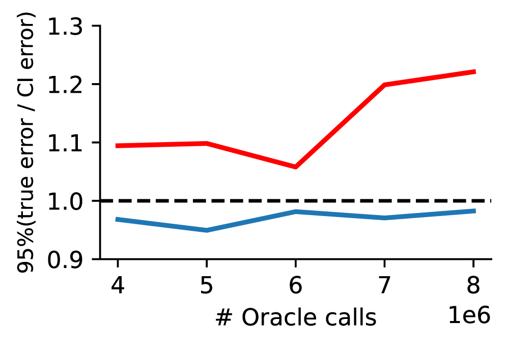
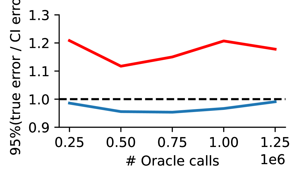
Metric. We use the ratio between the true error and the CI bounds as our evaluation metric. Given a query with a groundtruth result $\mu$, an estimated result $\hat{\mu}$, and a confidence interval $[l,u]$, the error ratio is calculated as: $\frac{|\hat{\mu}-\mu|}{|u-l|/2}$.

According to the definition of a CI, a valid 95% CI must include the true value with a probability of 95%. Consequently, the probability that the true error falls within the CI bounds should be at least 95%. Thus, for a method to provide valid CIs, the 95th percentile of the ratio between the true error and the CI bounds must not exceed 1.

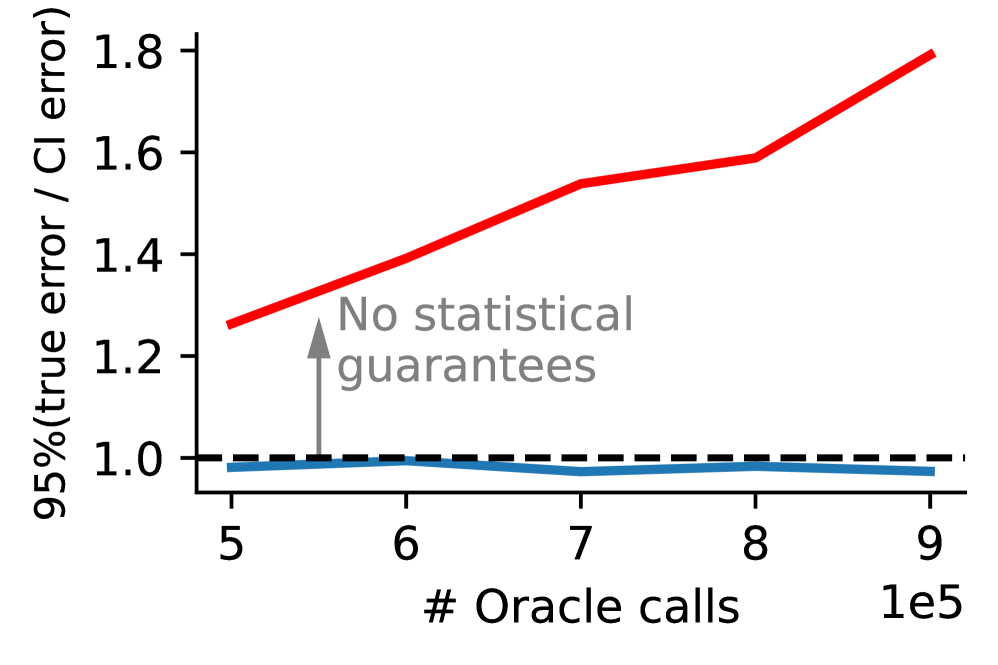
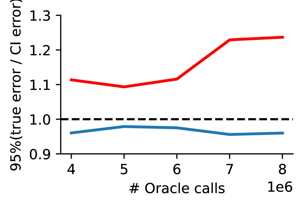
BaS Achieves Statistical Guarantees. We present the results for Blocking and BaS across various Oracle budgets in Figure 5. For each Oracle budget, we repeated the experiments 500 times. As shown, BaS consistently achieves 95th percentile error ratios of less than 1, indicating the validity of provided CIs. In contrast, Blocking fails to achieve valid CIs for every query, leading to true errors that are up to 79% higher than the CI errors.

We observe that the error ratio of Blocking increases as we increase the Oracle budget. This trend is expected because of the inherent bias of Blocking: it determines the data to execute Oracle through a similarity score threshold. Even when the similarity threshold is calibrated on a validation dataset, Blocking can still ignore positive pairs in the evaluation dataset, resulting in inherently biased estimation results. As the Oracle budget increases, the true error of Blocking decreases and converges to an unknown inherent bias, while the width of the CI approaches to zero. Consequently, when the Oracle budget is sufficiently large, true errors can be smaller than CI errors, causing invalid CIs. BaS resolves this problem by incorporating sampling algorithms to provide unbiased or asymptotically unbiased estimations, leading to valid CIs.

Figure 6. BaS maintains valid CIs even under extreme conditions, including low Oracle budgets (e.g., 1,000) and small pilot sample sizes (e.g., 0.1%).

(a) Company-COUNT

(b) Quora-AVG

(c) Webmasters-SUM

(d) Roxford-COUNT

(e) Flickr30K-COUNT

(f) VeRi-AVG

(g) Ecomm-Q7-COUNT

(h) Movie-Q5-AVG

(i) Movie-Q6-MAX

(j) Ecomm-Q8-MIN

(k) Ecomm-Q9-MEDIAN

(l) Ecomm-Q10a-GroupBy (3 tables)

(m) Ecomm-Q10-COUNT (3 tables)

(n) Ecomm-Q11-COUNT (4 tables)

(o) Company-Scale-COUNT (6 tables)

(p) Roxford-Scale-COUNT

Figure 7. BaS consistently reduces RMSE across a diverse workload. It outperforms baselines in linear aggregators (7(a)–7(h)), extreme aggregators (7(i) and 7(j)), MEDIAN (7(k)), GroupBy (7(l)), multi-table join (7(m)–7(o)), and large-scale join queries (7(o) and 7(p)). BaS remains robust in both rare-event (Low Selectivity) and dense (High Selectivity) scenarios.

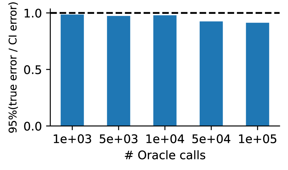
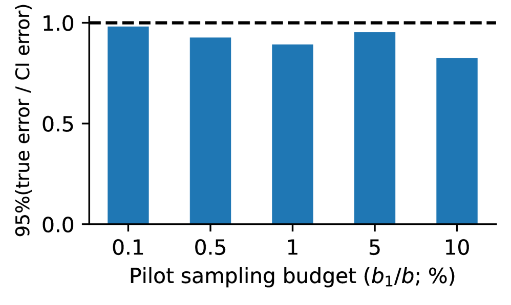
BaS Achieves Statistical Guarantees Under Limited Budgets. We show that our asymptotic statistical guarantees hold under limited budgets. In the left part of Figure 6, we report the maximum error ratio across all datasets. We show that BaS maintains valid CIs even when the oracle budget is as low as 1,000. These results empirically validate the robustness of the bootstrap-t method used in BaS, ensuring reliability even in small-budget scenarios. In right part of Figure 6, we show this validity holds regardless of the pilot sample size (varying from 0.1% to 10% of the budget). Intuitively, this is because the size of the pilot sample does not affect the derivation of confidence intervals, thus not affecting our statistical guarantees.

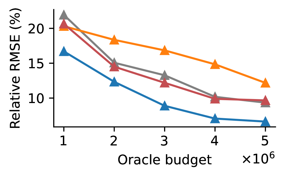
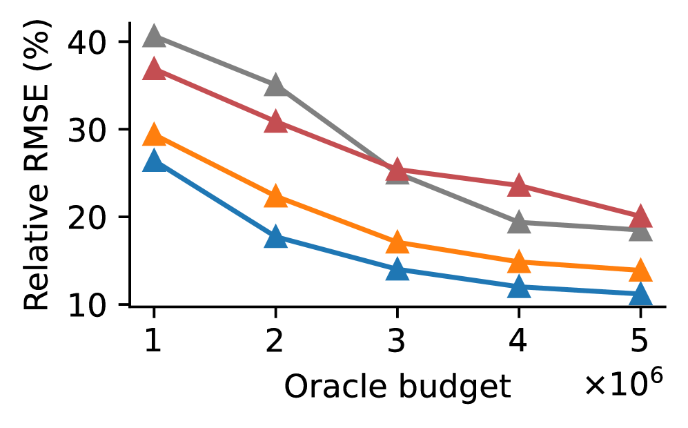
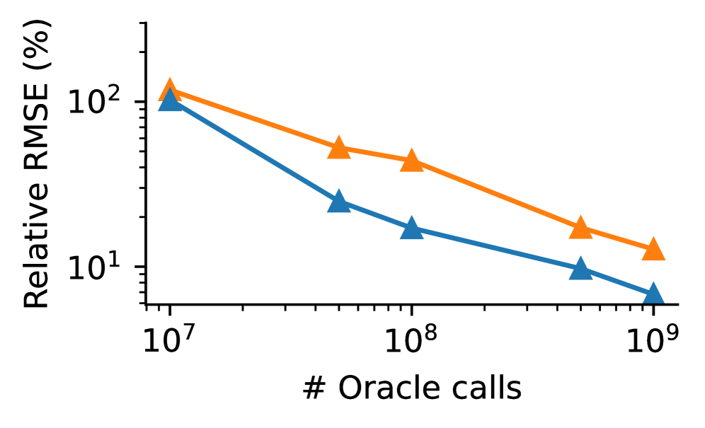
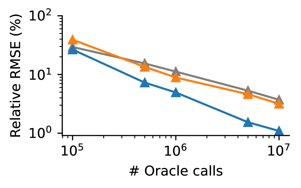
7.3. End-to-end Performance

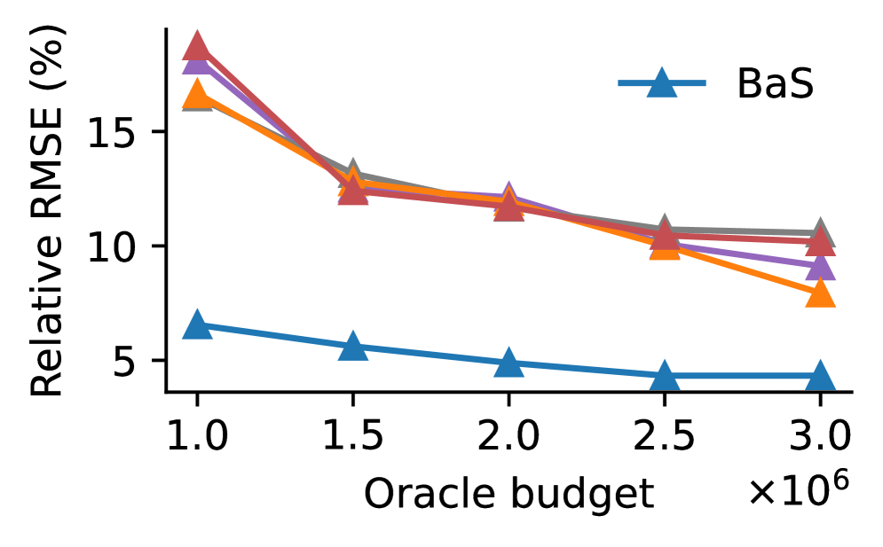
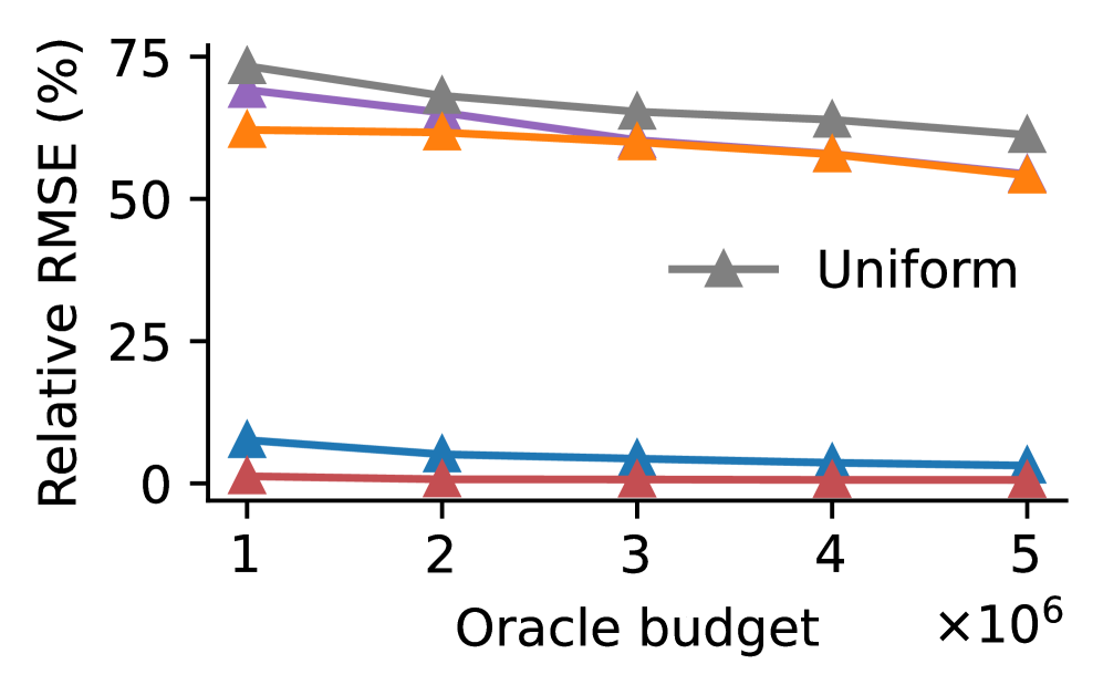
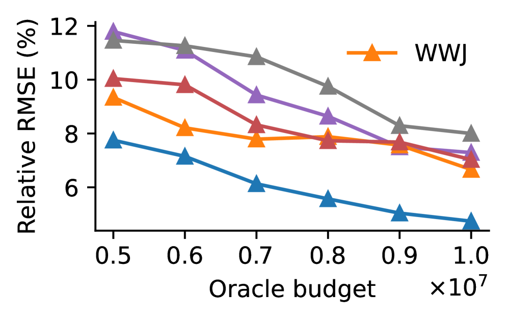
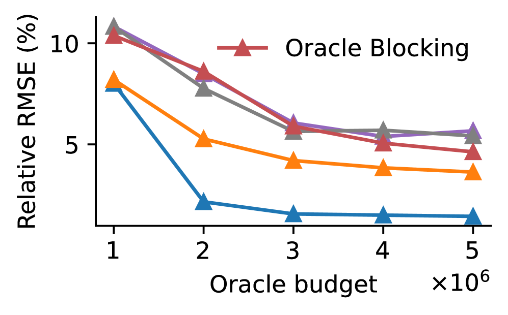
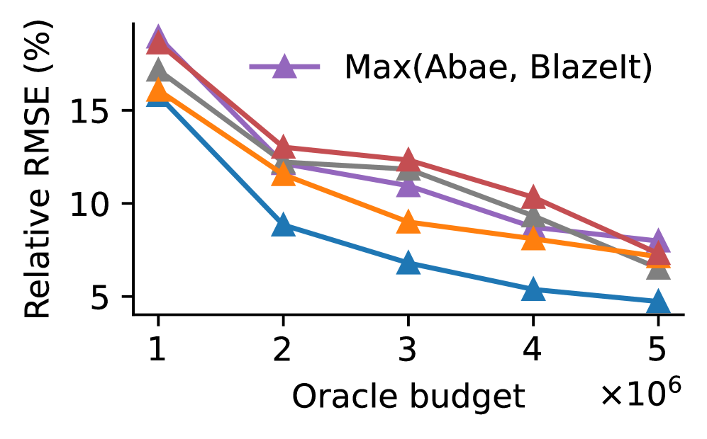
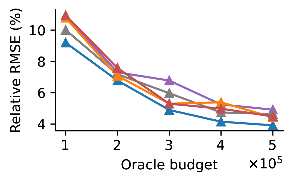
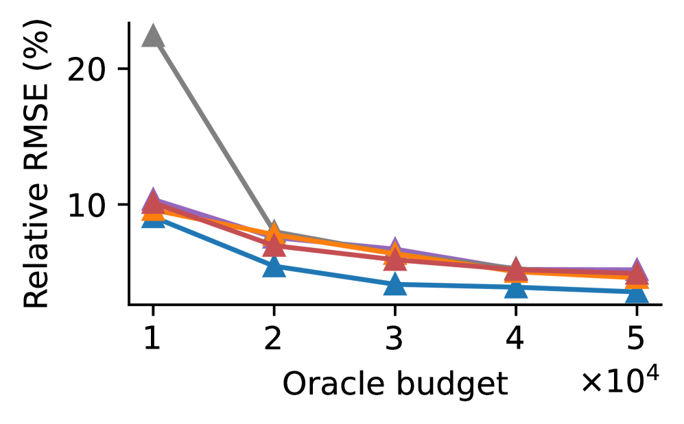
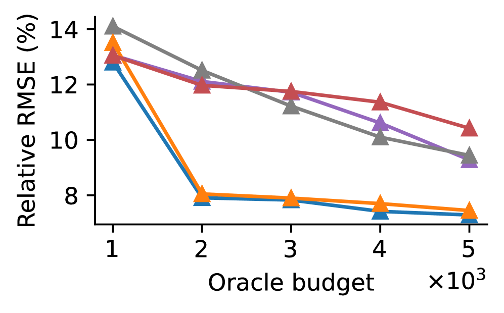
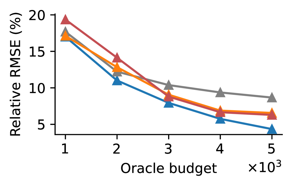
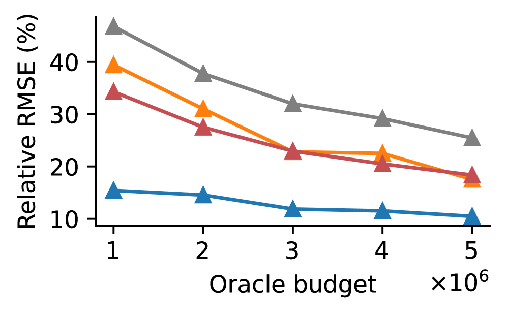
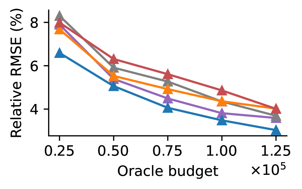
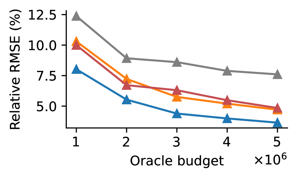
We analyze end-to-end performance on a diverse workload including real-world analytical joins, SemBench semantic queries, and multi-way joins. We report the average relative RMSE over 100 repetitions with a maximum blocking ratio $\alpha=20\%$.

BaS Improves Overall Estimation Errors. As shown in Figure 7, BaS reduces estimation errors by 1.04–19.5$\times$ compared to the best performing baseline among Uniform, Abae, and BlazeIt. Compared to WWJ, BaS achieves similar or lower estimation errors by up to 17.2$\times$. Except for Quora, BaS reduces errors by up to 2.2$\times$ compared to Oracle Blocking. This improvement is due to the relatively low Oracle threshold to achieve valid confidence intervals. While Oracle Blocking can be more efficient if positive and negative tuples are well distinguished by similarity scores (as in the case of Quora), determining the Oracle threshold requires exhaustive execution of the Oracle, making it prohibitively expensive.

BaS Reduces Estimation Errors Across Selectivities. We categorize results by join selectivity to demonstrate BaS’s adaptability:

1. Low-Selectivity ($<0.001$): On datasets with rare matches (Fig. 7(a)–7(e), 7(j), and 7(l)–7(p)), BaS significantly outperforms all baselines by up to 19.5$\times$. For the 6-way Company-Scale join (selectivity $5\times 10^{-10}$), Uniform sampling failed to retrieve sufficient positive samples to form an estimate, while BaS maintained low error.

2. High-Selectivity ($0.001-0.5$): In high-density scenarios (Fig. 7(f)–7(i). and 7(k)) where blocking offers little theoretical advantage, BaS demonstrates robustness. It adaptively allocates budget towards sampling, preventing the performance regression observed in Blocking. BaS achieves errors 1.05–2.5$\times$ lower than baselines and matches WWJ.

BaS Improves Real-World Multi-Way Joins. We evaluated scalability using real-world 3-way (Ecomm-Q10), 4-way (Ecomm-Q11), and synthetic 6-way (Company-Scale) joins. As shown in Figure 7(m)–7(o), BaS reduces error by 1.4–2.1$\times$ compared to Uniform and WWJ, while Abae and BlazeIt do not natively support multi-way joins. This performance gap highlights the critical role of blocking in large search spaces. As the number of joined tables increases, the density of valid join paths decreases, causing inefficient sampling.

BaS Improves MAX, MIN, MEDIAN, and GroupBy Queries. To demonstrate general applicability of BaS, we evaluated non-linear aggregators and GroupBy queries. We show that BaS reduces estimation error by up to 1.4$\times$ for MEDIAN (Fig. 7(k)), 2.0$\times$ for MAX (Fig. 7(i)), and 3.0$\times$ for MIN (Fig. 7(j)). For GroupBy queries (Fig. 7(l)), BaS reduces the mean estimation error across groups by up to 2.1$\times$ compared to baselines, demonstrating its utility for OLAP-style analytics.

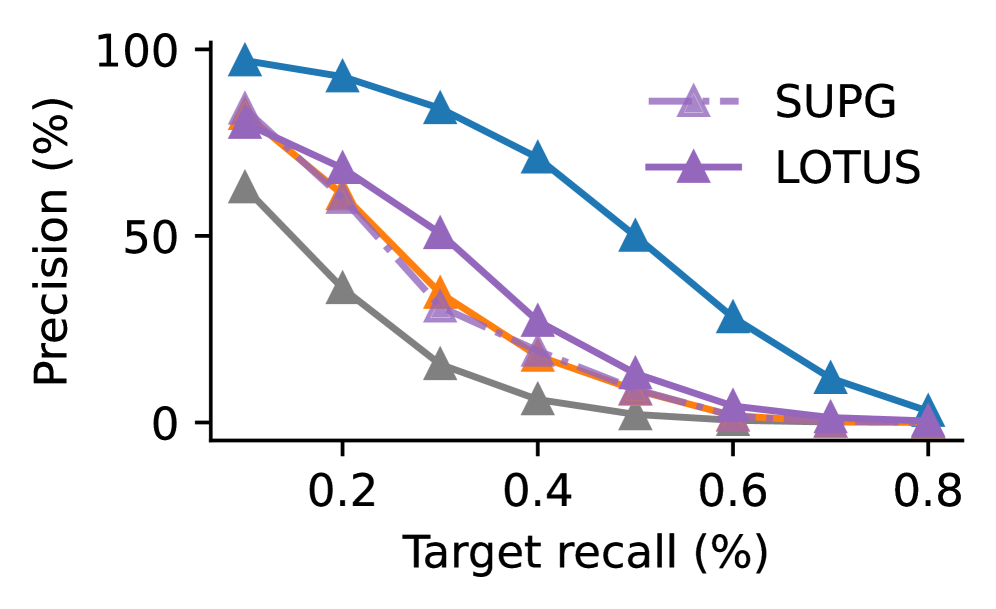
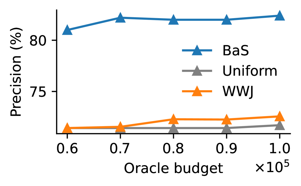
BaS Improves Selection Queries. We compared BaS against LOTUS (Patel et al., 2025) on selection queries (Fig. 8(a)). On a selection query based on the Company dataset, while both methods satisfy the recall target with 95% confidence, BaS achieves significantly higher precision, improving by 2.6–43.8% over LOTUS and 3.0–68.6% over Uniform. In addition, we show that WWJ achieves performance similar to SUPG (dotted purple line), empirically validating that WWJ shares the same statistical characteristics as SUPG for selection queries. Furthermore, for a TopK heavy-hitter query based on Ecomm-Q11 with recall guarantees (95% confidence), where LOTUS lacks native support, BaS improves precision by 9.6–10.7% over baselines. This indicates that BaS’s variance-optimal allocation is effective not only for aggregation, but for high-precision retrieval.

7.4. Application of Approximate COUNT: Join Order Optimization

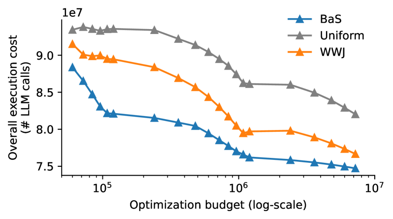
We applied BaS to the problem of join order optimization for exactly executing a multi-way semantic join query (Ecomm-Q11 of SemBench), where cardinality estimation errors can lead to execution costs 80$\times$ higher than optimal. By integrating BaS with the DPccp enumeration algorithm (Moerkotte and Neumann, 2006), we generate more accurate cardinality estimates for sub-joins. As shown in Figure 9, the improved COUNT estimation from BaS allows the optimizer to identify efficient execution plans, reducing total execution cost by up to 12.7% compared to plans generated using Uniform or WWJ estimates.

7.5. Ablation Study

We empirically validate the theoretical result in Section 6 that BaS converges to the optimal allocation. To achieve this, we compare the adaptive allocation with the optimal allocation and the worst allocation. To approximate the optimal and worst allocations, we executed BaS with fixed blocking ratios ranging from 10% to 50%. For example, a fixed blocking ratio of 10% means we directly execute Oracle on pairs with top 10% similarity scores while applying WWJ on the rest. For each ratio, we repeated experiments 100 times.

(a) BaS achieves up to 43% higher precision than LOTUS while maintaining the same recalls guarantees.

(b) BaS improves precision on TopK queries by up to 10% over baselines, while LOTUS does not support TopK with guarantees

Figure 8. BaS extends to improve selection queries.

Figure 9. Application of approximate COUNT to join optimization: By providing accurate cardinality estimates, BaS enables the query optimizer to select better join orders, reducing the execution cost of Ecomm-Q11 by 12.7%.

Figure 10. BaS determines near-optimal allocations.

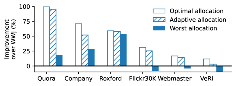
In Figure 10, we show the improvements of BaS using optimal, adaptive, and worst allocations over WWJ. We calculate the improvement as the relative reduction of RMSE. As shown, BaS with adaptive allocations achieves improvements that are only 1.61-18.9% (7.04% on average) less compared to BaS with optimal allocations. In contrast, BaS with the worst allocations underperforms (i.e., negative improvements) by up to 98.4% compared to WWJ and up to 99.9% compared to BaS with optimal allocations.

7.6. Sensitivity Analysis

We analyze the sensitivity of BaS in terms of the quality of embedding models, strategies to use the similarity scores as sampling weights, and the maximum blocking ratio $\alpha$.

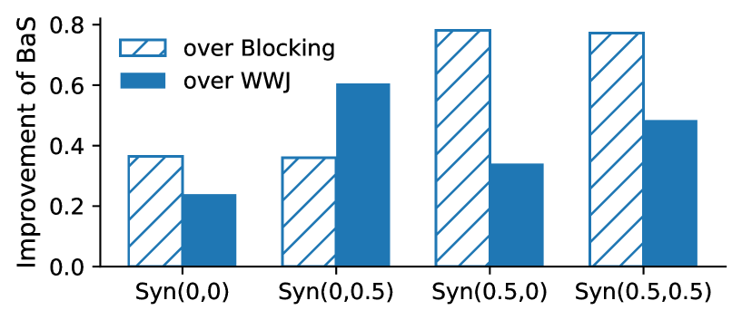
Impact of False Negatives and False Positives. We examined the impact of embedding quality using synthetic datasets with controlled False Negative Rates (FNR) and False Positive Rates (FPR). As shown in Figure 12, when FNR and FPR reach 50%, BaS outperforms baselines by more than 20%. Specifically, BaS dominates Blocking when FNR is high (by correcting for missed matches via sampling) and dominates WWJ when FPR is high (by avoiding the overweighting of false positives).

Impact of the Embedding Quality. We executed algorithms on the Company dataset with 9 more embeddings, including traditional textual similarity (Corley and Mihalcea, 2005; Ramos and others, 2003), encoder-only embedding models (Reimers and Gurevych, 2019), and large-scale embedding models (Lee et al., 2024; Xiao et al., 2023; DunZhang, 2024; Rui* et al., 2024; Li et al., 2023b; OpenAI, 2024). For each embedding method, we executed WWJ and BaS 100 times with an Oracle budget of 1,000,000. In Figure 11, we demonstrate the performance of BaS, WWJ, and Uniform with various embeddings on the Company dataset with an Oracle budget of 1,000,000 and a maximum blocking ratio of 20%. As shown, BaS consistently outperforms Uniform and WWJ across all embeddings. We find that BaS benefits from improved performance with better embeddings.

Figure 11. BaS consistently outperforms Uniform and WWJ across various types of embeddings.

Figure 12. On the synthstic dataset Syn(FN, FP), BaS outperforms baselines even as embedding quality degrades. BaS is particularly effective compared to Blocking when False Negatives (FN) are high, and compared to WWJ when False Positives (FP) are high.

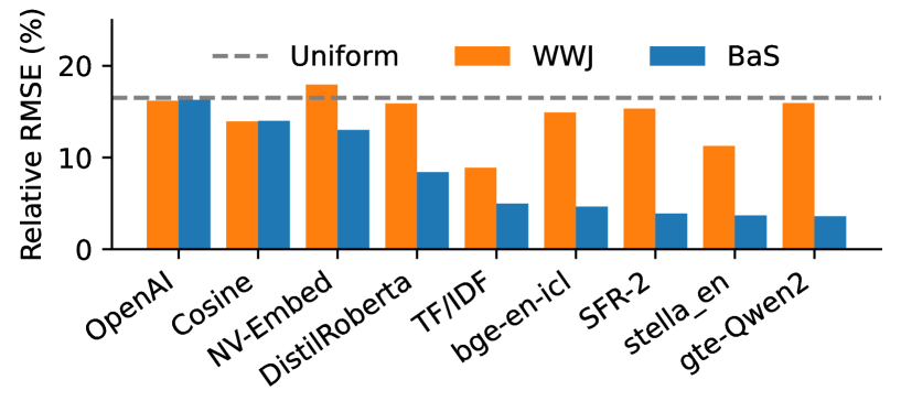
Furthermore, we find that traditional TF-IDF sometimes outperforms modern dense embeddings (e.g., OpenAI). This counter-intuitive result is caused by the specific join semantics of the Company dataset, which requires high lexical precision (e.g., distinguishing a radio company from a television company), a task where traditional methods excel by strictly penalizing token mismatches. In contrast, dense embeddings prioritize semantic relatedness, often clustering non-matching companies from the same industry, creating extra false positives (e.g., 99% FPR for OpenAI vs. 27% for TF-IDF). Therefore, traditional methods or embedding models with instructional prompts (e.g., gte-Qwen2 (Li et al., 2023b) and stella_en (DunZhang, 2024)) work better on this dataset. Nevertheless, BaS provides statistical guarantees regardless of the embedding’s quality.

(a) $\alpha$ vs relative RMSE for the Webmasters dataset.

(b) Weight exponent vs relative RMSE for the Company dataset.

Figure 13. Sensitivity of BaS in terms of $\alpha$ and the weight exponents. BaS consistently outperforms baselines.

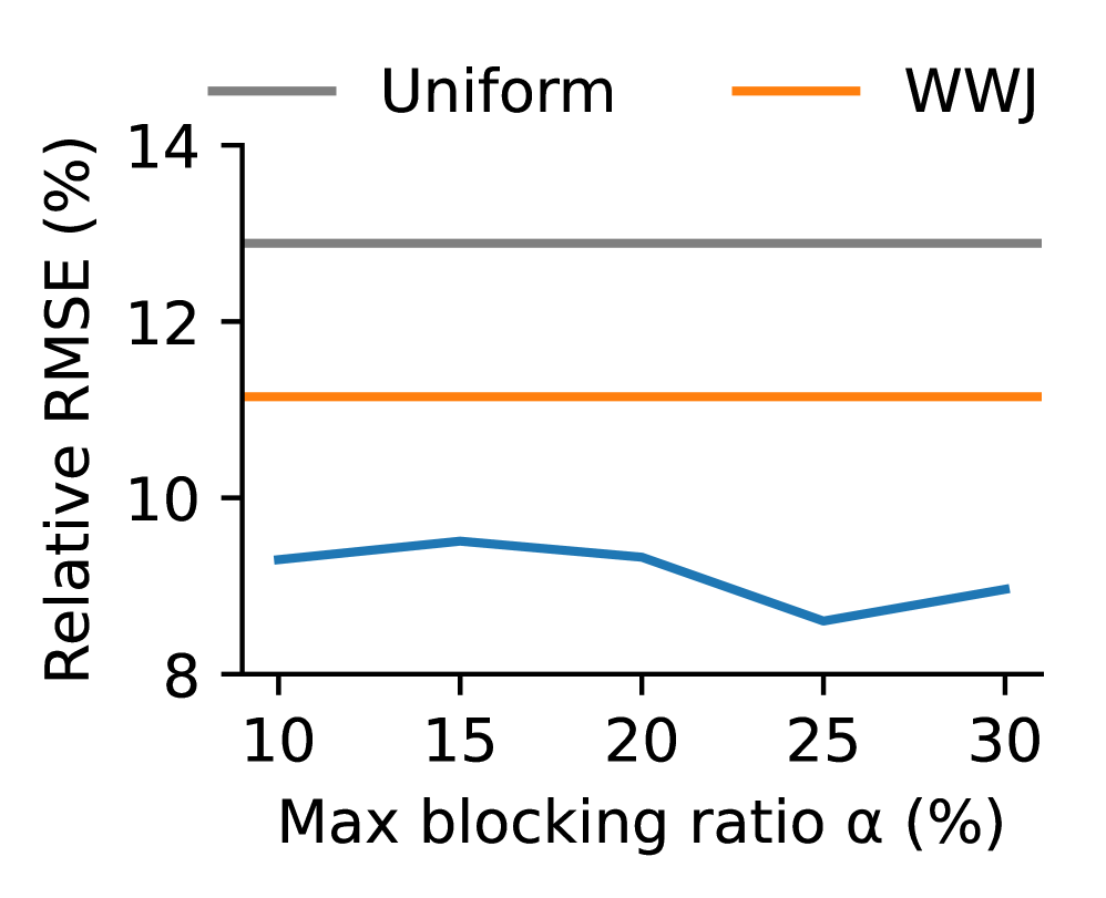
Impact of the Maximum Blocking Ratio ($\alpha$). We executed BaS with maximum blocking ratios ($\alpha$) ranging from 10% to 30% on the Flickr30K datasets. For each value of $\alpha$, we repeated experiments 100 times and measured the relative RMSE. As shown in Figure 13(a), the RMSE of BaS fluctuates by 9.5-14.2% compared with the optimal one. Despite the fluctuation, BaS consistently outperforms baselines, demonstrating that BaS is insensitive to $\alpha$.

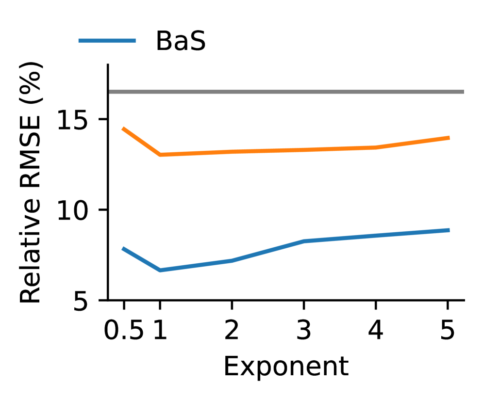
Impact of the Weight Exponents. We executed WWJ and BaS on the Company dataset with different weight exponents. For example, the exponent=0.5 means that the sampling weight and budget allocation is proportional to the square root of the similarity score. For each exponent, we repeated experiments 100 times and measure the relative RMSE. As shown in Figure 13(b), BaS achieves relatively better performance with exponent equal to 1 and consistently outperforms baselines.

8. Related Work

We draw inspiration from classic join optimization algorithms and leverages recent advancements in EM and AQP. We summarize the relevant literature on these areas.

Optimization of approximate join queries. Joins are fundamental but notoriously expensive operations in relational database management systems (Abiteboul et al., 1995; Maier, 1983). To optimize and accelerate join queries with structured data, various algorithms and systems are developed in both offline and online scenarios.

Prior work developed offline sampling algorithms to address the challenge that joining uniform samples does not constitute an independent sample of the join (Chaudhuri et al., 1999; Zhao et al., 2018; Huang et al., 2019). Specifically, researchers proposed the Stratified-Universe-Bernoulli sampling that achieves the theoretical optimal sampling performance within a constant factor (Huang et al., 2019). For joins with specific types, prior work proposed precomputed synopses and histogram method (Sitzmann and Stuckey, 2000; Acharya et al., 1999). To accelerate join queries in the online scenario, prior work proposed ripple join (Haas and Hellerstein, 1999). Wander Join improved the sampling efficiency using indices and random walks (Li et al., 2016).

Recently, for unstructured data, researchers have focused on efficient implementations of the semantic join operator (Patel et al., 2025; Trummer, 2025). Notably, Trummer (2025) proposes a batch-oriented block nested loop algorithm that optimizes prompt construction to evaluate multiple row pairs in a single LLM invocation. This line of work addresses the physical execution efficiency of the join operator. In contrast, BaS addresses the logical approximate execution of such queries via reducing variance. These approaches are highly complementary. BaS optimizes which pairs to check, while (Trummer, 2025) reduces the cost of checking those pairs, particularly in the dense blocking regime.

Entity Matching. EM seeks to identify common objects across datasets (Elmagarmid et al., 2006; Papadakis et al., 2020). Earlier approaches have modeled EM problems as similarity joins (Chaudhuri et al., 2006; Wang et al., 2011). However, EM is prohibitively expensive due to pair-wise comparisons (Shen et al., 2014). The blocking method is developed to reduce the number of pair-wise comparisons. Traditional blocking methods relied on heuristics and expert knowledge to develop rule-based block constructions, such as suffix arrays (De Vries et al., 2009; Papadakis et al., 2015), sorted neighborhood (Puhlmann et al., 2006; Yan et al., 2007), and sorted block (Draisbach and Naumann, 2011).

Recent advances in ML models, especially LLMs, have facilitated learning-based methods in EM systems (Li et al., 2021b, 2020b; Mudgal et al., 2018; Thirumuruganathan et al., 2021). Existing work proposed to use language models for textual data embedding, classification (Li et al., 2021b, 2020b; Mudgal et al., 2018), and blocking (Thirumuruganathan et al., 2021). Additionally, recent work improved the robustness of learning-based methods using data augmentation (Akbarian Rastaghi et al., 2022).

AQP for unstructured data. Recent work addressed AQP for unstructured data using machine learning models. To reduce the cost of executing expensive machine learning models, prior work leveraged approximate indexes (Hsieh et al., 2018), binary classifiers (Lu et al., 2018), and specialized models (Kang et al., 2017) for AQP without statistical guarantees. Furthermore, advancements including query-driven object tracking algorithms and segmentation-based tracking queries, further reduced the query cost. To provide guarantees on accuracy, existing work used proxy models with control variate to process aggregation and limit queries on video frames (Kang et al., 2019), importance sampling to process selection queries (Kang et al., 2020), and stratified sampling to process aggregation queries (Kang et al., 2021).

Join operations have been commonly used for unstructured data in prior AQP systems for unstructured data (Jo and Trummer, 2024; Liu et al., 2024; Patel et al., 2025). However, prior work either focused on join with structured join keys (Jo and Trummer, 2024; Liu et al., 2024), which is orthogonal to our work, or applies calibration techniques without statistical guarantees (Patel et al., 2025).

9. Conclusion

In this work, we propose Weighted Wander Join and Blocking-augmented Sampling to approximately process analytical join queries over unstructured data with statistical guarantees. We address the inaccuracy of embedding models by integrating sampling and blocking, and propose an adaptive allocation algorithm to minimize the errors. Theoretically, we prove the optimality and superiority of BaS. Our evaluation results demonstrate that BaS outperforms baselines by up to 21$\times$, saving costs by up to 188$\times$ on real-world datasets. These results highlight the potential of embeddings and cost-effective algorithms in analyzing unstructured data with joins.

10. Acknowledgements

We are grateful to the CloudLab for providing computing resources for experiments (Duplyakin). We thank Kaimeng Zhu and Siheng Pan for their help during the initial implementation and experimentation of this work. This research was supported in part by Google.

Appendix A Cost and Latency Analysis

Figure 14. Decomposition of the average (log-scale) latency for CPU computation of BaS.

In this section, we analyze the cost of executing ML models and the latency of our algorithm. We use Quora as an example to show that the cost of executing embedding models is minimal relative to running the Oracle. We observe similar results on other datasets. Consider OpenAI’s text-embedding-3-large model, the most expensive among the embedding models evaluated in Section 7.6. It costs $0.05 to generate embeddings for all data records using the batch API. In contrast, labeling all data pairs using the state-of-the-art prompt template (Narayan et al., 2022) would cost $78,848 with GPT-4o or $4,730 with GPT-4o mini using the batch API. This is about six orders of magnitude more expensive than generating embeddings.

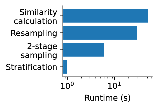
We then analyze the latency of the CPU computations by measuring the single-thread runtime of BaS on Intel 8562Y+ with 200 GB memory. As shown in Figure 14, similarity calculation and resampling contribute to 95% of the latency. The overall latency on CPU is lower than 90 seconds, which is minimal compared to executing the Oracle on GPUs or relying on human labelers.

Appendix B Theoretical Justification

In this section, we prove that BaS converges to the optimal allocation at the rate of $\mathcal{O}(1/\sqrt{b_{1}})$ and asymptotically outperforms or matches the standalone sampling algorithm. In addition, we prove that BaS be extended to accelerate approximate selection join queries with recall guarantees.

Table 1. Summary of Notation

Symbol	Description
$D$	stratified dataset of data tuples in the cross product of join tables
$W$	normalized similarity scores of tuples in $D$
$O$	Oracle
$g$	attribute where the aggregate is computed
$b,b_{1},b_{2}$	Oracle budget of the overall procedure, pilot sampling, and sampling+blocking execution
$p$	confidence
$\alpha$	maximum blocking ratio
$K$	number of strata
$\widehat{\texttt{COUNT}},\widehat{\texttt{SUM}},\widehat{\texttt{AVG}},\widehat{\texttt{AGG}}$	estimated aggregate for the entire dataset, sampling regime (with a subscript $s$), and blocking regime (with a subscript $b$)
$l,u$	lower, upper bound of the confidence interval
$\mathcal{O}(\cdot)$	Bachmann-Landau big-O notation
$\beta,\beta^{*},\hat{\beta}^{*}$	the allocated strata to blocking that is given, optimal, and estimated
$n^{(1)}_{i},n_{i}$	assigned Oracle budget for stratum $i$ during pilot sampling and blocking+sampling execution
$\sigma_{i}^{2},\hat{\sigma}_{i}^{2}$	(estimated) sampling variance of stratum $i$
$\mu,\hat{\mu}$	(estimated) expectation of stratum $i$
$S^{(1)}_{i},S_{i}$	sampled data tuples from stratum $i$ during pilot sampling and blocking+sampling
$t_{j}$	t-statistic of the $j$-th resampling iteration
$\tilde{D},\tilde{D}^{(s)}$	the set of matching tuples of the entire dataset or the sampling regime

B.1. Setup

In this section, we describe BaS in detail as a setup for the theoretical analysis. We will go over the entire procedure of BaS, including stratification, pilot sampling, blocking, sampling, and resampling.

Inputs and Outputs. BaS takes as inputs the cross product of tables $D$, the similarity scores $W$, the Oracle $O$, the overall Oracle budget $b$ divided for pilot sampling ($b_{1}$) and bloking+sampling execution ($b_{2}$), the confidence $p$, the maximum blocking ratio $\alpha$, and the number of strata $K$. BaS outputs an estimated aggregate $\hat{\mu}$ and its confidence interval $[l,u]$.

Stratification. We divide $D$ into a maximum blocking regime and a minimum sampling regime ($D_{0}$). The maximum blocking regime contains tuples with the top $\alpha\cdot b$ similarity scores, where $\alpha$ is a parameter between 0 and 1 to control the size of the maximum blocking regime. Next, we stratify the maximum blocking regime into $K$ strata ($D_{1},\ldots,D_{K}$) with equal sizes. The number of strata $K$ is automatically determined to ensure that each stratum has an Oracle budget of at least 1,000.

Pilot Sampling. For each stratum, we execute WWJ to obtain a pilot sample $S_{i}^{(1)}$. The Oracle budget for the stratum $i$ in the pilot sampling is calculated as

(8) $$n^{(1)}_{i}=b_{1}\cdot\frac{\sum_{s\in D_{i}}W(s)}{\sum_{s\in D}W(s)}$$

We can estimate the sampling variance as

$$\hat{\sigma}^{2}_{i}=\frac{1}{n^{(1)}-1}\sum_{s\in S^{(1)}_{i}}\left(\frac{g(s)O(s)}{W(s)|D_{i}|}-\left(\frac{1}{n_{i}^{(1)}}\sum_{s^{\prime}\in S^{(1)}_{i}}\frac{g(s^{\prime})O(s^{\prime})}{W(s^{\prime})|D_{i}|}\right)\right)^{2}W(s)$$

Given an allocation $\beta$, we can then estimate the MSE of BaS for a SUM aggregate as follows

$$\widehat{MSE}_{\texttt{SUM}}(D,\beta,W,b_{2})=\sum_{\begin{subarray}{c}0\leq i\leq k,i\notin\beta\end{subarray}}\frac{|D_{i}|^{2}}{n_{i}}\cdot\hat{\sigma}_{i}^{2}$$

where $n_{i}$ is the assigned Oracle budget for stratum $i$ in the stage of blocking+sampling execution, calculated as

$$n_{i}=\begin{cases}(b_{2}-\sum_{j\in\beta}|D_{i}|)\cdot\frac{\sum_{s\in D_{i}}W(s)}{\sum_{1\leq j\leq K,j\notin\beta}\sum_{s\in D_{j}}W(s)}&i\notin\beta\\ |D_{i}|&i\in\beta\\ \end{cases}$$

Next, we obtain the estimated optimal allocation by solving the following optimization problem using iterative methods.

$$\hat{\beta}^{*}=\mathop{\arg\min}_{\beta\subset\{1,\ldots,K\}}\widehat{MSE}_{\texttt{SUM}}(D,\beta,W,b_{2})$$

Blocking+Sampling. Given the optimal allocation $\hat{\beta}^{*}$, we use the Oracle budget $b_{1}$ to execute the Oracle on the strata that are allocated to the blocking regime. On the remaining strata, we execute WWJ to obtain a sample using the remaining Oracle budget. We can obtain the sample $S_{i}$ on the stratum $i$ that is allocated to sampling. Then, we merge the result of all strata and the results of pilot sampling to estimate the aggregate. Specifically, we estimate the aggregate as follows:

$$\widehat{\texttt{COUNT}}_{s}=\frac{1}{\sum_{i\notin\hat{\beta}^{*}}n_{i}}\sum_{i\notin\hat{\beta}^{*}}\sum_{s\in S_{i}}\frac{O(s)}{W(s)|D_{i}|},\ \texttt{COUNT}_{b}=\sum_{i\in\hat{\beta}^{*}}\sum_{s\in D_{i}}O(s)$$

$$\widehat{\texttt{COUNT}}_{s}=\frac{1}{\sum_{i\notin\hat{\beta}^{*}}n_{i}}\sum_{i\notin\hat{\beta}^{*}}\sum_{s\in S_{i}}\frac{g(s)O(s)}{W(s)|D_{i}|},\ \texttt{COUNT}_{b}=\sum_{i\in\hat{\beta}^{*}}\sum_{s\in D_{i}}g(s)O(s)$$

$$\widehat{\texttt{COUNT}}=\widehat{\texttt{COUNT}}_{s}+\texttt{COUNT}_{b},\ \widehat{\texttt{SUM}}=\widehat{\texttt{SUM}}_{s}+\texttt{SUM}_{b}$$

$$\widehat{\texttt{AVG}}=\left(\widehat{\texttt{SUM}}_{s}+\texttt{SUM}_{b}\right)\Big/\left(\widehat{\texttt{COUNT}}_{s}+\texttt{COUNT}_{b}\right)$$

Resampling. We apply the bootstrap-t resampling scheme to calculate the CI (Hall, 1988). The bootstrap-t scheme estimates the standard error $\frac{\hat{\mu}-\mu}{\sigma}$ (i.e., t-statistic) of the underlying distribution by resampling existing samples. To process aggregation queries, we first calculate the mean and standard deviation of the estimator. Next, we use sampling with replacement to resample from all existing samples ($S^{(1)}\cup S$). We calculate the t-statistic of the $j$-th iteration as follows.

$$t_{j}=\frac{\widehat{\texttt{AGG}}_{j}-\widehat{\texttt{AGG}}}{\hat{\sigma}_{j}}$$

where $\widehat{\texttt{AGG}}_{j}$ and $\hat{\sigma}_{j}$ are the estimated aggreagte and standard deviation on the $j$-th resample. To achieve statistical guarantees, we repeat the resampling a sufficient number of times (e.g., 1000). Finally, we use the percentiles of resampled t-statistics to construct the CI, that is

$$l=\widehat{\texttt{AGG}}-\mathrm{Percentile}\left(t,\frac{1-p}{2}\right),\quad u=\widehat{\texttt{AGG}}-\mathrm{Percentile}\left(t,1-\frac{1-p}{2}\right)$$

B.2. BaS Converges to the Optimal Allocation

Theorem B.1.

The MSE with the estimated minimizer $\hat{\beta}^{*}$ converges to that with the true minimizer $\beta^{*}$ with the rate $\mathcal{O}\left(1/\sqrt{b_{1}}\right)$:

$$\frac{MSE(D,\widehat{\beta}^{*},W,b_{2})-MSE(D,\beta^{*},W,b_{2})}{MSE(D,\beta^{*},W,b_{2})}=\mathcal{O}\left(\frac{1}{\sqrt{b_{1}}}\right)$$

Proof.

We first show the estimated MSE converges to the true MSE. To achieve that, we establish the convergence rate of the sample mean $\hat{\mu}_{i}$ and variance $\hat{\sigma}_{i}^{2}$ for stratum $i$ because MSE estimations are calculated with summations, multiplications, and divisions of basic estimators $\hat{\mu}_{i},\hat{\sigma}_{i}^{2}$.

We construct the concentration inequality for the sample mean $\hat{\mu}_{i}$ and sample variance $\hat{\sigma}_{i}^{2}$ of each stratum $D_{i},i=0,\ldots,K$. Given the i.i.d. sample, we can bound the relative errors of $\hat{\mu}_{i}$ and $\hat{\sigma}_{i}^{2}$ with Chebeyshev’s Inequality, where the variance of an i.i.d. sample variance is calculated as $Var\left[\hat{\sigma}_{i}^{2}\right]=\frac{2\sigma_{i}^{4}}{n_{i}-1}$ (Berger and Casella, 2001).

(9) $$\mathbb{P}\left[\left|\frac{\mu_{i}-\hat{\mu}_{i}}{\mu_{i}}\right|\leq\frac{\sigma_{i}}{\mu_{i}\sqrt{\delta n_{i}^{(1)}}}\right] \geq 1-\frac{\delta}{2}$$

(10) $$\mathbb{P}\left[\left|\frac{\sigma_{i}^{2}-\hat{\sigma}_{i}^{2}}{\sigma_{i}^{2}}\right|\leq\sqrt{\frac{2}{\delta(n_{i}^{(1)}-1)}}\right] \geq 1-\frac{\delta}{2}$$

where $\delta$ is a small probability.

Since $n_{i}^{(1)}$ is linearly related to the Oracle budget $b_{1}$ (Eq. 8), we have the following big-$\mathcal{O}$ notations showing the convergence rate that holds with high probability.

(11) $$\frac{\mu_{i}-\hat{\mu}_{i}}{\mu_{i}}=\mathcal{O}\left(b_{1}^{-1/2}\right),\quad\frac{\sigma_{i}^{2}-\hat{\sigma}_{i}^{2}}{\sigma_{i}^{2}}=\mathcal{O}\left(b_{1}^{-1/2}\right)$$

Next, we show the convergence rate of relative error is preserved after summations, multiplications, and divisions. Namely, for unbiased estimators $\mu_{1}$ and $\mu_{2}$ with relative error converging to 0 with a rate of $\mathcal{O}\left(b_{1}^{-1}\right)$ ($t>0$), we have Equations 12 - 14.

$$(\mu_{1}+\mu_{2})-(\hat{\mu}_{1}+\hat{\mu}_{2}) =\mu_{1}\cdot\mathcal{O}\left(b_{1}^{-1}\right)+\mu_{2}\cdot\mathcal{O}\left(b_{1}^{-1}\right)$$

(12) $$=(\mu_{1}+\mu_{2})\cdot\mathcal{O}\left(b_{1}^{-1}\right)$$

$$\mu_{1}\mu_{2}-\hat{\mu}_{1}\hat{\mu}_{2} =\mu_{1}\mu_{2}-\mu_{1}\left(1+\mathcal{O}\left(b_{1}^{-1}\right)\right)\mu_{2}\left(1+\mathcal{O}\left(b_{1}^{-1}\right)\right)$$

$$=\mu_{1}\mu_{2}\left(\mathcal{O}\left(b_{1}^{-1}\right)+\mathcal{O}\left(b_{1}^{-2t}\right)\right)$$

(13) $$=\mu_{1}\mu_{2}\mathcal{O}\left(b_{1}^{-1}\right)$$

$$\mu^{-1}-\hat{\mu}^{-1} =\mu^{-1}\hat{\mu}^{-1}(\hat{\mu}-\mu)$$

$$=\mu^{-2}\left(1+\mathcal{O}\left(b_{1}^{-1}\right)\right)^{-1}\mu\mathcal{O}\left(b_{1}^{-1}\right)$$

(14) $$=\mu^{-1}\mathcal{O}\left(b_{1}^{-1}\right)$$

Therefore, given the convergence rate of basic estimators (Eq. 11) and propagation rules (Eq. 12-14), the relative error of our optimization objective converges to 0 with the same rate $\mathcal{O}\left(b_{1}^{-1/2}\right)$, with high probability. Namely, the following probabilistic bound holds for any $\beta\subset\{1,\ldots,K\}$ with a high probability of $1-\delta/2$

(15) $$\mathbb{P}\left[\left|\frac{MSE_{\texttt{AGG}}(D,\beta,W,b_{2})-\widehat{MSE}_{\texttt{AGG}}(D,\beta,W,b_{2})}{MSE_{\texttt{AGG}}(D,\beta,W,b_{2})}\right|\leq\frac{C}{\sqrt{b_{1}}}\right]\geq 1-\frac{\delta}{2}$$

where $C$ is a constant independent of $n$. Based on Equation 15, we can derive the following bound for MSE that holds with a high probability of $1-\delta/2$.

$$\frac{1}{1+\frac{C}{\sqrt{n}}}\widehat{MSE}_{\texttt{AGG}}(\beta)\leq MSE_{\texttt{AGG}}(\beta)\leq\frac{1}{1-\frac{C}{\sqrt{n}}}\widehat{MSE}_{\texttt{AGG}}(\beta)$$

where we omit the parameters $D,W,b_{2}$ for simplicity.

We then derive the upper bound of the difference between the MSE of BaS and the optimal MSE. Given the estimated minimizer $\hat{\beta}^{*}$ and the true minimizer $\beta^{*}$, we can establish the following upper bound of the difference between $MSE_{\texttt{AGG}}(\hat{\beta}^{*})$ and $MSE_{\texttt{AGG}}(\beta^{*})$.

(16) $$MSE_{\texttt{AGG}}(\hat{\beta}^{*})-MSE_{\texttt{AGG}}(\beta^{*})\leq\frac{1}{1-\frac{C_{1}}{\sqrt{n}}}\widehat{MSE}_{\texttt{AGG}}(\hat{\beta}^{*})-MSE_{\texttt{AGG}}(\beta^{*})$$

(17) $$\leq\frac{1}{1-\frac{C_{1}}{\sqrt{n}}}\widehat{MSE}_{\texttt{AGG}}(\beta^{*})-MSE_{\texttt{AGG}}(\beta^{*})$$

(18) $$\leq\frac{1}{1-\frac{C_{1}}{\sqrt{n}}}\left(1+\frac{C_{2}}{\sqrt{n}}\right)MSE_{\texttt{AGG}}(\beta^{*})-MSE_{\texttt{AGG}}(\beta^{*})$$

(19) $$=\frac{C_{1}+C_{2}}{\sqrt{n}-C_{1}}MSE_{\texttt{AGG}}(\beta^{*})$$

where inequalities 16 and 18 apply the probabilistic inequalities of $MSE_{\texttt{AGG}}(\hat{\beta}^{*})$ and $MSE_{\texttt{AGG}}(\beta^{*})$ respectively, inequality 17 is due to the definition of estimated minimizer $\hat{\beta}^{*}$, and $C_{1},C_{2}$ are constants from the probabilistic inequalities.

Finally, we derive the upper bound of the relative error of the optimization objective that holds with high probability.

$$\frac{MSE_{\texttt{AGG}}(\hat{\beta}^{*})-MSE_{\texttt{AGG}}(\beta^{*})}{MSE_{\texttt{AGG}}(\beta^{*})}\leq\frac{C_{1}+C_{2}}{\sqrt{n}-C_{1}}$$

This upper bound shows that the relative error between the MSE with estimated minimizer $\hat{\beta}^{*}$ and the MSE with actual minimizer $\beta^{*}$ converges to 0 at the rate $\mathcal{O}\left(b_{1}^{-1/2}\right)$ with high probability. ∎

B.3. BaS Outperforms or Matches WWJ

Theorem B.2.

If there exists an allocation $\beta$ such that the following two conditions hold

(20) $$\mathbb{E}_{s\in\tilde{D}^{(s)}}\left[\frac{1/|\tilde{D}^{(s)}|}{W(s)}\right] \leq\mathbb{E}_{s\in D}\left[\frac{1/|D|}{W(s)}\right]$$

(21) $$\frac{|\tilde{D}^{(s)}|^{2}}{b_{2}^{(s)}} \leq\frac{|D|^{2}}{b}$$

BaS outperforms WWJ asymptotically, i.e.,

$$MSE_{\texttt{SUM}}=C\cdot MSE^{(w)}_{\texttt{SUM}}+\mathcal{O}\left(b_{1}^{-1}b_{2}^{-1/2}\right)$$

where $C$ is a coefficient less than 1:

$$C<\frac{|\tilde{D}^{(s)}|^{2}\big/b_{2}^{(s)}}{|\tilde{D}|^{2}/b}\frac{\mathbb{E}_{s\in\tilde{D}^{(s)}}\left[\frac{1/|\tilde{D}^{(s)}|}{W(s)}\right]}{\mathbb{E}_{s\in\tilde{D}}\left[\frac{1/|\tilde{D}|}{W(s)}\right]}\leq 1$$

Otherwise, BaS matches WWJ asymptotically, i.e.,

$$MSE_{\texttt{SUM}}\leq MSE^{(w)}_{\texttt{SUM}}+\mathcal{O}\left(b_{1}^{-1}b_{2}^{-1/2}\right)$$

Proof.

We first derive the ratio between the MSE of BaS and importance sampling, given a deterministic allocation $\beta$. The MSe of BaS for a SUM aggregate can be calculated as follows.

$$MSE_{\texttt{SUM}}$$

$$=\sum_{i\notin\beta}\frac{1}{n_{i}}\left(\mathbb{E}_{s\sim W,s\in D_{i}}\left[\left(\frac{g(s)O(s)}{W(s)}\right)^{2}\right]-\left(\mathbb{E}_{s\sim W,s\in D_{i}}\left[\frac{g(s)O(s)}{W(s)}\right]\right)^{2}\right)$$

$$=\frac{1}{b_{2}^{(s)}}\sum_{i\notin\beta}\left(|D_{i}|\mathbb{E}\left[\frac{g(s)^{2}O(s)}{r_{i}W(s)}\right]-\frac{1}{r_{i}}\left(|D_{i}|\mathbb{E}\left[g(s)O(s)\right]\right)^{2}\right)$$

where

$$b_{2}^{(s)}=b_{2}-\sum_{i\in\beta}|D_{i}|,\quad r_{i}=\frac{\sum_{s\in D_{i}}W(s)}{\sum_{j\notin\beta}\sum_{s\in D_{j}}W(s)}$$

Assuming the independence of the SUM column $g(\cdot)$ and the oracle results $O(\cdot)$, we can further simplify the expression of MSE as follows.

$$MSE_{\texttt{SUM}}=\frac{1}{b_{2}^{(s)}}\cdot$$

$$\left(\mathbb{E}\left[g(s)^{2}\right]\sum_{i\notin\beta}\left(|D_{i}|\mathbb{E}\left[\frac{O(s)}{r_{i}W(s)}\right]\right)-\frac{\mathbb{E}[g(s)]^{2}}{r_{i}}\sum_{i\notin\beta}\left(|D_{i}|\mathbb{E}\left[O(s)\right]\right)^{2}\right)$$

We notice that $r_{i}$ unweights the proxy scores over a stratum into the proxy scores over the whole sampling regions. In this case, we merge $r_{i}W(s)$ as $W(s)$. Furthermore, we can simplify the sum of the expectations of strata into the expectation of the whole sampling region.

$$MSE_{\texttt{SUM}}=\frac{1}{b_{2}^{(s)}}\cdot$$

$$\left(|D|\cdot\mathbb{E}\left[g(s)^{2}\right]\cdot\mathbb{E}\left[\frac{O(s)}{W(s)}\right]-\frac{\mathbb{E}[g(s)]^{2}}{r_{i}}\sum_{i\notin\beta}\left(|D_{i}|\mathbb{E}\left[O(s)\right]\right)^{2}\right)$$

Next, we rewrite the expectations over all tuples with expectations over matching tuples by evaluating the oracle results $O(\cdot)$.

$$MSE_{\texttt{SUM}}$$

$$=\frac{1}{b_{2}^{(s)}}\left(\mathbb{E}\left[g(s)^{2}\right]\cdot\left|\tilde{D}^{(s)}\right|\cdot\mathbb{E}_{s\in\tilde{D}^{(s)}}\left[\frac{1}{W(t)}\right]-\mathbb{E}[g(s)]^{2}\sum_{i\notin\beta}\frac{|\tilde{D}_{i}|^{2}}{r_{i}}\right)$$

$$=\frac{\left|\tilde{D}^{(s)}\right|}{b_{2}^{(s)}}\left(\mathbb{E}\left[g(s)^{2}\right]\mathbb{E}_{s\in\tilde{D}^{(s)}}\left[\frac{1}{W(t)}\right]-\mathbb{E}[g(s)]^{2}\sum_{i\notin\beta}q_{i}\left|\tilde{D}^{(s)}_{i}\right|\right)$$

where

$$q_{i}=\frac{\left|\tilde{D}^{(s)}_{i}\right|}{\sum_{j\notin\beta}\left|\tilde{D}^{(s)}_{j}\right|}\bigg/r_{i}$$

We rewrite the $MSE$ of WWJ for a SUM aggregate.

$$MSE_{\texttt{SUM}}^{(w)} =\frac{1}{b}\left(\mathbb{E}_{s\sim W}\left[\left(\frac{g(s)O(s)}{W(s)}\right)^{2}\right]-\left(\mathbb{E}_{s\sim W}\left[\frac{g(s)O(s)}{W(s)}\right]\right)^{2}\right)$$

$$=\frac{1}{b}\left(|D|\cdot\mathbb{E}\left[\frac{g(s)^{2}O(s)}{W(s)}\right]-\left(|D|\cdot\mathbb{E}\left[g(s)O(s)\right]\right)^{2}\right)$$

$$=\frac{1}{b}\left(\mathbb{E}\left[g(s)^{2}\right]\cdot|D|\cdot\mathbb{E}\left[\frac{O(s)}{W(s)}\right]-|\tilde{D}|^{2}\cdot\mathbb{E}[g(s)]^{2}\right)$$

$$=\frac{|\tilde{D}|}{b}\left(\mathbb{E}\left[g(s)^{2}\right]\mathbb{E}_{s\in\tilde{D}}\left[\frac{1}{W(t)}\right]-\mathbb{E}[g(s)]^{2}|\tilde{D}|\right)$$

We take the ratio between the $MSE$ of BaS and that of WWJ. We assume the variance of SUM-column in the sampling region is the same as that for all tuples.

$$\frac{MSE_{\texttt{SUM}}}{MSE_{\texttt{SUM}}^{(w)}}$$

$$=\frac{|\tilde{D}^{(s)}|\big/b_{2}^{(s)}}{|\tilde{D}|/b}\frac{\mathbb{E}\left[g(s)^{2}\right]\mathbb{E}_{s\in\tilde{D}^{(s)}}\left[\frac{1}{W(s)}\right]-\mathbb{E}[g(s)]^{2}\sum_{i\notin\beta}q_{i}\left|\tilde{D}^{(s)}_{i}\right|}{\mathbb{E}\left[g(s)^{2}\right]\mathbb{E}_{s\in\tilde{D}}\left[\frac{1}{W(s)}\right]-\mathbb{E}[g(s)]^{2}|\tilde{D}|}$$

$$=\frac{|\tilde{D}^{(s)}|\big/b_{2}^{(s)}}{|\tilde{D}|/b}\frac{\mathbb{E}_{s\in\tilde{D}^{(s)}}\left[\frac{1}{W(s)}\right]-\frac{\mathbb{E}[g(s)]^{2}}{\mathbb{E}[g(s)^{2}]}\sum_{i\notin\beta}q_{i}\left|\tilde{D}^{(s)}_{i}\right|}{\mathbb{E}_{s\in\tilde{D}}\left[\frac{1}{P(s)}\right]-\frac{\mathbb{E}[g(s)]^{2}}{\mathbb{E}[g(s)^{2}]}|\tilde{D}|}$$

$$=\frac{|\tilde{D}^{(s)}|\big/b_{2}^{(s)}}{|\tilde{D}|/b}\frac{\mathbb{E}_{s\in\tilde{D}^{(s)}}\left[\frac{1}{W(t)}\right]-\frac{1}{1+CV_{g}}\sum_{i\notin\beta}q_{i}\left|\tilde{D}^{(s)}_{i}\right|}{\mathbb{E}_{s\in\tilde{D}}\left[\frac{1}{W(s)}\right]-\frac{1}{1+CV_{g}}|\tilde{D}|}$$

where $CV_{g}$ is the coefficient of variation of the SUM-column $g(\cdot)$,

$$CV_{g}=\frac{Var[g(s)]}{E[g(s)]^{2}}$$

We apply Holder’s Inequality to obtain an upper bound to the effect of stratification on the MSE as follows.

$$\sum_{i\notin\beta}q_{i}\left|\tilde{D}^{(s)}_{i}\right|=\frac{1}{|\tilde{D}^{(s)}|}\sum_{i\notin\beta}\frac{\left|\tilde{D}^{(s)}_{i}\right|^{2}}{r_{i}}=\frac{1}{|\tilde{D}^{(s)}|}\left(\sum_{i\notin\beta}\frac{\left|\tilde{D}^{(s)}_{i}\right|^{2}}{r_{i}}\right)\left(\sum_{i\notin\beta}r_{i}\right)$$

$$\geq\frac{1}{|\tilde{D}^{(s)}|}\left(\sum_{i\notin\beta}\frac{\left|\tilde{D}^{(s)}_{i}\right|}{\sqrt{r_{i}}}\sqrt{r_{i}}\right)^{2}=\left|\tilde{D}^{(s)}\right|$$

Therefore, the ratio has the following upper bound.

$$\frac{MSE_{\texttt{SUM}}}{MSE_{\texttt{SUM}}^{(w)}} \leq\frac{|\tilde{D}^{(s)}|\big/b_{2}^{(s)}}{|\tilde{D}|/b}\frac{\mathbb{E}_{s\in\tilde{D}^{(s)}}\left[\frac{1}{W(s)}\right]-\frac{1}{1+CV_{g}}|\tilde{D}^{(s)}|}{\mathbb{E}_{s\in\tilde{D}}\left[\frac{1}{W(s)}\right]-\frac{1}{1+CV_{g}}|\tilde{D}|}$$

$$=\frac{|\tilde{D}^{(s)}|^{2}\big/b_{2}^{(s)}}{|\tilde{D}|^{2}/b}\frac{\mathbb{E}_{s\in\tilde{D}^{(s)}}\left[\frac{1/|\tilde{D}^{(s)}|}{W(s)}\right]-\frac{1}{1+CV_{g}}}{\mathbb{E}_{s\in\tilde{D}}\left[\frac{1/|\tilde{D}|}{W(s)}\right]-\frac{1}{1+CV_{g}}}$$

If the following condition holds

(22) $$\mathbb{E}_{s\in\tilde{D}^{(s)}}\left[\frac{1/|\tilde{D}^{(s)}|}{W(s)}\right]\leq\mathbb{E}_{s\in\tilde{D}}\left[\frac{1/|\tilde{D}|}{W(s)}\right],$$

we have the following upper bound for the ratio

$$\frac{MSE_{\texttt{SUM}}}{MSE_{\texttt{SUM}}^{(IS)}}<\frac{|\tilde{D}^{(s)}|^{2}\big/b_{2}^{(s)}}{|\tilde{D}|^{2}/b}\frac{\mathbb{E}_{s\in\tilde{D}^{(s)}}\left[\frac{1/|\tilde{D}^{(s)}|}{W(s)}\right]}{\mathbb{E}_{s\in\tilde{D}}\left[\frac{1/|\tilde{D}|}{W(s)}\right]}$$

Furthermore, if the matching tuples are sparse in the sampling region, i.e.,

(23) $$|\tilde{D}^{(s)}|^{2}\big/b_{2}^{(s)}<|\tilde{D}|^{2}/b$$

Then,

$$MSE_{\texttt{SUM}}=C\cdot{MSE_{\texttt{SUM}}^{(IS)}}$$

where $C$ is a coefficient less than 1,

$$C<\frac{\mathbb{E}_{s\in\tilde{D}^{(s)}}\left[\frac{1/|\tilde{D}^{(s)}|}{W(s)}\right]}{\mathbb{E}_{s\in\tilde{D}}\left[\frac{1/|\tilde{D}|}{W(s)}\right]}\leq 1$$

We then apply the Theorem B.1 to replace the MSE of BaS with deterministic allocation with the MSE of BaS with pilot sampling. Namely, we have the following approximation:

$$MSE_{\texttt{SUM}}(\hat{\beta}^{*}) =MSE_{\texttt{SUM}}(\beta^{*})\cdot\left(1+\mathcal{O}\left(b_{1}^{-1/2}\right)\right)$$

$$=C\cdot{MSE_{\texttt{SUM}}^{(w)}}\left(1+\mathcal{O}\left(b_{1}^{-1/2}\right)\right)$$

Since $MSE_{\texttt{SUM}}^{(w)}$ converges to 0 at the rate $\mathcal{O}\left(b^{-1}\right)$. Therefore, we conclude that if the conditions 22 and 23 hold, JoinML outperforms WWJ asymptotically. Namely,

(24) $$MSE_{\texttt{SUM}}(\hat{\beta}^{*})=C\cdot{MSE_{\texttt{SUM}}^{(IS)}}+\mathcal{O}\left(b_{1}^{-1/2}b^{-1}\right)$$

On the other hand, if the conditions 22 and 23 do not hold, we can set $\beta=\emptyset$, which will make the sampling region become the entire data tuples. In this case, the upper bound of the ratio will be 1. Namely,

$$MSE_{\texttt{SUM}}\leq MSE^{(IS)}_{\texttt{SUM}}$$

Taking Theorem B.1 into account, we will have the following upper bound for MSE of BaS.

$$MSE_{\texttt{SUM}} \leq MSE_{\texttt{SUM}}\left(1+\mathcal{O}\left(b_{1}^{-1/2}\right)\right)\leq MSE^{(w)}_{\texttt{SUM}}\left(1+\mathcal{O}\left(b_{1}^{-1/2}\right)\right)$$

(25) $$=MSE^{(w)}_{\texttt{SUM}}+\mathcal{O}\left(b_{1}^{-1/2}b^{-1}\right)$$

To conclude, we have shown that the MSE of BaS either outperforms (Eq. 24) or matches (Eq. 25) that of WWJ asymptotically. ∎

B.4. BaS for Selection Join Queries

Lemma B.3.

With a probability higher than $p$, we can achieve the overall recall target $\gamma$ if $\gamma_{s}$ satisfies

$$\gamma_{s}\geq\gamma-(1-\gamma)\frac{\texttt{COUNT}_{b}}{\mathrm{UB}(\texttt{COUNT}_{s},Var[\texttt{COUNT}_{s}],b,p)}$$

where

$$\mathrm{UB}(\mu,\sigma^{2},b,p)=\mu+\frac{\sigma}{\sqrt{b}}\sqrt{2\log\frac{2}{1-p}}$$

Proof.

We first show the upper bound of the number of matching tuples in the sampling region $\widehat{\texttt{COUNT}}_{s}$. Then, the required recall target $\gamma_{s}$ of the sampling region follows automatically.

Given an i.i.d. sample of size $n$ drawn from a population with mean $\mu$ and finite and non-zero variance $\sigma^{2}$, the upper bound of the sample mean can be estimated with normal approximation (Kang et al., 2020; Agarwal et al., 2014). Namely,

$$\mathbb{P}\left[\hat{\mu}\geq\mu+\frac{\sigma}{\sqrt{n}}\sqrt{2\log\frac{2}{1-p}}\right]\leq\frac{1-p}{2}$$

where $p$ is the confidence.

We rewrite the recall target of the sampling region $\gamma^{\prime}_{s}$ with the overall recall target $\gamma$ specified by the user.

$$\gamma_{s}=\frac{\gamma\left(\widehat{\texttt{COUNT}}_{s}+\widehat{\texttt{COUNT}}_{b}\right)-\widehat{\texttt{COUNT}}_{b}}{\widehat{\texttt{COUNT}}_{s}}=\gamma-(1-\gamma)\frac{\widehat{\texttt{COUNT}}_{b}}{\widehat{\texttt{COUNT}}_{s}}$$

We observe that $\gamma_{s}$ is monotonically increasing with respect to $\widehat{\texttt{COUNT}}_{s}$. Therefore, we use the upper bound of $\widehat{\texttt{COUNT}}_{s}$ to estimate the required $\gamma_{s}$ such that the user-specified overall recall target can be guaranteed with high probability. ∎

B.5. Bootstrap Validity

In this section, we show that bootstrap resampling is asymptotically valid for BaS, which is inspired by (Kang et al., 2021).

Overview. We summarize our approach as follows. Suppose that the sampling procedure with CDF $F_{0}$ leads to a sequence of random variables $X_{1},\ldots,X_{N}$, and $\theta$ is a statistical functional of $F_{0}$. If $\theta$ is Hadamard differentiable, the delta method of (Van der Vaart, 2000) will imply the validity of using bootstrap resampling for the CIs of $\theta$. In the rest of this section, we first define $\theta$ for BaS and derive the Hadamard differentiability of $\theta$.

Notation. We first define the notations for the derivation. Suppose $X_{i}=(P_{i},Y_{i})$ is a tuple drawn from the cross product of tables, where $P_{i}\in\{0,1\}$ indicates whether the tuple satisfy the join condition, $Y_{i}$ is the value to be SUM-ed or AVG-ed. We can define the statistical function $\theta$ for COUNT, SUM, and AVG as follows:

$$\theta_{f,\texttt{COUNT}}=\sum_{i}\frac{P_{i}}{N\cdot f(X_{i})},\quad\theta_{f,\texttt{SUM}}=\sum_{i}\frac{P_{i}\cdot Y_{i}}{N\cdot f(X_{i})},$$

$$\theta_{f,\texttt{AVG}}=\frac{\sum_{i}\frac{P_{i}\cdot Y_{i}}{N\cdot f(X_{i})}}{\sum_{i}\frac{P_{i}}{N\cdot f(X_{i})}}$$

where $f(\cdot)$ is a deterministic distribution denoting the sampling probability.

Theorem B.4.

Let $\dot{\theta}_{f,F_{0},\texttt{AGG}}\left(\mathbb{B}\right)$ be the converged distribution of the difference between the empirical and statistical distribution:

$$\sqrt{b}\left(\theta_{f,\texttt{AGG}}\left(\hat{F}_{b}\right)-\theta_{f,\texttt{AGG}}\left(F_{0}\right)\right)\xrightarrow{\mathcal{D}}\dot{\theta}_{f,F_{0},\texttt{AGG}}\left(\mathbb{B}\right)$$

where $b$ is the sample size, $F_{0}$ is the CDF of the population, and $\hat{F}_{b}$ is the empirical CDF of the observed sample. For any fixed sampling probability $f$ and aggregates $\texttt{AGG}\in\{\texttt{COUNT},\texttt{SUM},\texttt{AVG}\}$, we have the following convergence in distribution:

$$\sqrt{b}\left(\theta_{f,\texttt{AGG}}\left(\hat{F}_{b}^{*}\right)-\theta_{f,\texttt{AGG}}\left(\hat{F}_{b}\right)\right)\xrightarrow{\mathcal{D}}\dot{\theta}_{f,F_{0},\texttt{AGG}}\left(\mathbb{B}\right)$$

where $\hat{F}_{b}^{*}$ is the resampled CDF. Namely, the bootstrap is valid.

Proof.

According to Theorem 23.9 of (Van der Vaart, 2000), it is sufficient to show that $\theta_{f,\texttt{AGG}}$ is Hadamard differentiable.

For any $f$ with $\sum_{i}\frac{P_{i}}{f(X_{i})}\geq 0$, $\theta_{f,\texttt{COUNT}}$ is Hadamard differentiable. For any $f$ with $\sum_{i}\frac{P_{i}\cdot Y_{i}}{f(X_{i})}\geq 0$, $\theta_{f,\texttt{SUM}}$ is also Hadamard differentiable. For any join with non-empty results, $\sum_{i}\frac{P_{i}}{N\cdot f(X_{i})}$ is non-zero. Then, we apply the chain rule (Theorem 20.9, (Van der Vaart, 2000)) and show that $\theta_{f,\texttt{COUNT}}^{-1}$ is Hadamard differentiable. We then apply the product rule, implying that $\theta_{f,\texttt{AVG}}$ is Hadamard differentiable.

∎

Dataset	Modality	Table size	Cross product size	Positive rate	Oracle	Embedding model
Company	text	$1.0\times 10^{4}$, $1.0\times 10^{4}$	$1.0\times 10^{8}$	$3.6\times 10^{-5}$	Human label	MiniLM (Wang et al., 2020)
Quora	text	$6.0\times 10^{4}$	$3.6\times 10^{9}$	$1.1\times 10^{-6}$	Human label	MiniLM (Wang et al., 2020)
Webmasters	text	$1.8\times 10^{4}$	$3.2\times 10^{8}$	$4.6\times 10^{-5}$	Human label	MiniLM (Wang et al., 2020)
Roxford	image	$70$, $1.0\times 10^{6}$	$7.0\times 10^{7}$	$7.8\times 10^{-5}$	Human label	SuperGlobal (Shao et al., 2023)
VeRi	image	$2.1\times 10^{4}$, $2.8\times 10^{4}$	$6.0\times 10^{8}$	$1.4\times 10^{-3}$	Human label	TransReID (He et al., 2021)
Flickr30K	text, image	$3.2\times 10^{4}$, $1.6\times 10^{5}$	$5.1\times 10^{9}$	$3.1\times 10^{-5}$	Human label	BLIP (Li et al., 2022)
Ecomm-Q7	text	$8.1\times 10^{3}$	$6.5\times 10^{7}$	$8.1\times 10^{-3}$	Human label	MiniLM (Wang et al., 2020)
Ecomm-Q8	text, image	$3.0\times 10^{2}$, $4.4\times 10^{4}$	$1.3\times 10^{7}$	$2.3\times 10^{-5}$	Human label	CLIP (Radford et al., 2021)
Ecomm-Q9	image	$6.1\times 10^{3}$	$3.7\times 10^{7}$	$2.4\times 10^{-2}$	Human label	CLIP (Radford et al., 2021)
Ecomm-Q10	text, image	$4.6\times 10^{2}$, $9.0\times 10^{2}$, $4.2\times 10^{3}$	$1.7\times 10^{9}$	$2.1\times 10^{-5}$	Human label	CLIP (Radford et al., 2021)
Ecomm-Q11	text, image	$370$, $600$, $2.0\times 10^{3}$, $2.9\times 10^{3}$	$1.3\times 10^{12}$	$5.6\times 10^{-6}$	Human label	CLIP (Radford et al., 2021)
Movie-Q5,Q6	text	$7.6\times 10^{2}$	$5.7\times 10^{5}$	$5.0\times 10^{-1}$	Human label	Flair (Akbik et al., 2019)
Company-Scale	text	$1.0\times 10^{4},3\times 10^{3},300,25,25,20$	$1.1\times 10^{14}$	$3.0\times 10^{-10}$	Human label	MiniLM (Wang et al., 2020)
Roxford-Scale	image	$70,1.0\times 10^{7}$	$7\times 10^{8}$	$7.8\times 10^{-5}$	Human label	SuperGlobal (Shao et al., 2023)
Syn	N/A	$1.0\times 10^{4}$, $1.0\times 10^{4}$	$1.0\times 10^{8}$	$1\times 10^{-4}$	Synthetic	Synthetic (Kang et al., 2020)

Table 2. Summary of datasets, Oracle, and embedding models.

Appendix C Datasets and Queries

In this section, we introduce the construction details of the datasets and queries used in evaluation.

C.1. Dataset Collection and Construction

Quora. Widely used to evaluate the sentence paraphrasing task in the NLP community, the Quora dataset contains single-sentence questions from the forum quora.com, labeled by human (25; H. Jiang, P. He, W. Chen, X. Liu, J. Gao, and T. Zhao (2020)). We repurpose it to a paraphrasing detection task with the self-join operation.

WebMaster. Collected for knowledge mining tasks and studied for duplication detection tasks, the WebMaster dataset contains long posts from the network question partition of the QA forum stackexchange.com for developers, labeled by human (Bacchelli, 2013; Zhang et al., 2015). We repurpose it to a duplication detection task.

Company. As widely used to evaluate the EM systems, the Company dataset has two lists of long descriptions about companies, where the matched companies between the lists are labeled by human (Mudgal et al., 2018; Li et al., 2020b). We use it as a two-table join task. Additionally, we split the two tables in six tables with sizes: 20, 25, 25, 300, 3,000, and 10,000, simulating the join “barebones” of TPC-H Q7—the largest join evaluated by Wander Join (Li et al., 2016).

VeRi. Proposed to evaluate the vehicle re-identification algorithms, the VeRi dataset contains images of vehicles captured by multiple cameras on different crossroads, where the identical vehicles are labeled by human (Liu et al., 2016, 2017). We repurpose it to a two-table join task.

Flickr30K. Proposed to evaluate the image-to-sentence models, the Flickr30K dataset contains the image entities and sentence mentions from the Flickr.com, where the matched images and sentences are labeled by human (Plummer et al., 2017). We repurpose it to a two-table join task.

Roxford. Proposed to evaluate object retrieval and visual search algorithms, the Roxford (Oxford Buildings) dataset consists of images depicting famous architectural landmarks in Oxford collected from Flickr, where images representing the same building are labeled by human (Radenović et al., 2018). We repurpose it to a two-table join task for visual landmark identification. Additionally, we uniformly scale up the dataset to construct a query involving 10 million rows.

SemBench. As a benchmark for semantic query processing engines, SemBench contains semantic queries from six application domains. From the queries involving join operations, we collected ones that have at least one join predicate about the joint semantics across tables. When there are semantic operators other than join (e.g., filtering), we preprocess these in order to isolate the evaluation of joins. Additionally, we introduced two modified versions of queries to cover GroupBy and TopK queries.

Syn. Designed to stress-test join algorithms under varying noise levels, this dataset consists of two tables of size 10,000 with synthetic similarity scores. We assign ground-truth matches randomly based on selectivity and sample scores from distinct Beta distributions to distinguish matches ($Beta(5,0.5)$) from non-matches ($Beta(0.5,5)$), following prior work (Kang et al., 2020). We subsequently inject noise by inverting the score distributions for subsets of pairs to simulate precise False Positive and False Negative rates.

C.2. Query Semantics

We define the semantics of the evaluated queries as follows, utilizing domain-specific semantic predicates.

Company (Entity Resolution). Estimating the number of overlapping entities between two distinct corporate data sources (e.g., Wikipedia vs. DBPedia) based on textual descriptions.

⬇

SELECT COUNT(*)

FROM wiki_companies AS c1

JOIN dbpedia_companies AS c2

ON NL(‘Company 1: {c1.description} and Company 2: {c2.description} are the same company.’)’

Quora (Paraphrase Detection). Analyzing data quality by computing the average difference in character length between questions marked as semantic duplicates.

⬇

SELECT AVG(ABS(q1.char_len - q2.char_len))

FROM quora_questions AS q1

JOIN quora_questions AS q2

ON NL(’Question␣1:␣{q1.text}␣and␣Question␣2:␣{q2.text}␣are␣paraphrased␣from␣each␣other.’)

WHERE q1.id < q2.id

Webmasters (Redundancy Impact). Calculating the total community effort (number of answers) wasted on duplicate forum posts.

⬇

SELECT SUM(p1.answer_count)

FROM forum_posts AS p1

JOIN forum_posts AS p2

ON NL(’Post␣1:␣{p1.post}␣and␣Post␣2:␣{p2.post}␣are␣duplicated.’)

WHERE p1.id != p2.id

Roxford (Visual Search). Counting the number of images in a gallery that depict the same building/landmark as the query images.

⬇

SELECT COUNT(*)

FROM oxbuild_gallery AS g

JOIN oxbuild_queries AS q

ON NL(’Two␣images␣show␣the␣same␣landmark:␣{g.image}␣{q.image}’)

Flickr-30K (Cross-Modal Retrieval). Measuring the alignment between an image dataset and a caption dataset by counting valid image-text pairs.

⬇

SELECT COUNT(*)

FROM flickr_images AS img

JOIN flickr_captions AS cap

ON NL(’Caption␣{cap.text}␣describes␣the␣image␣{img.image}’)

VeRi (Traffic Analytics). Calculating the average transit time for vehicles traveling between two different camera locations (Re-ID).

⬇

SELECT AVG(cam2.timestamp - cam1.timestamp)

FROM surveillance_cam_A AS cam1

JOIN surveillance_cam_B AS cam2

ON NL(’Two␣images␣show␣the␣same␣vehicle:␣{cam1.image}␣{cam2.image}’)

Ecomm-Q7. Counting matching pairs for budget-friendly fashion items based on strict brand and category alignment.

⬇

SELECT COUNT(*)

FROM fashion_styles AS t1

JOIN fashion_styles AS t2

ON NL(’Product␣1␣{t1.text}␣and␣Product␣2␣{t2.text}␣have␣the␣same␣brand␣and␣type.’)

WHERE t1.price <= 500 AND t2.price <= 500

Ecomm-Q8. Calculating the minimum price of the product which has an image and have extensive textual descriptions (exceeding 3,000 characters).

⬇

SELECT t.id, i.id

FROM fashion_text AS t

JOIN fashion_images AS i

ON NL(’The␣product␣description:␣{t.text}␣describes␣the␣image␣{i.image}’)

WHERE LENGTH(t.description) >= 3000

Ecomm-Q9. Calculating the median price difference of two budget-friendly (¡ 800), single-colored fashion items that share identical primary color and category.

⬇

SELECT MEDIAN(ABC(t1.price - t2.price))

FROM fashion_items AS t1

JOIN fashion_items AS t2

ON NL(’Two␣images␣show␣the␣products␣with␣the␣same␣color␣and␣category:␣{t1.image}␣{t2.image}’)

WHERE t1.price < 800 AND t1.baseColour IN (’Black’, ’Blue’, ’Red’, ’White’, ’Orange’, ’Green’)

Ecomm-Q10. Counting the number of coherent three-piece outfits (Footwear, Bottomwear, Topwear) by linking budget-friendly items (¡ 1000) that share the same brand and base color.

⬇

SELECT COUNT(*)

FROM footwear AS s

JOIN bottomwear AS b

ON NL(’Two␣images␣show␣the␣products␣with␣the␣same␣brand␣and␣color:␣{s.image}␣{b.image}’)

JOIN topwear AS t

ON NL(’Two␣images␣show␣the␣products␣with␣the␣same␣brand␣and␣color:␣{b.image}␣{t.image}’)

WHERE s.price <= 1000 AND s.baseColour IN (’Black’, ’Blue’, ’Red’, ’White’)

Ecomm-Q10a. Counting the number of coherent three-piece outfits (Footwear, Bottomwear, Topwear) by linking budget-friendly items (¡ 1000) that share the same brand and base color and grouping the results by color.

⬇

SELECT COUNT(*)

FROM footwear AS s

JOIN bottomwear AS b

ON NL(’Two␣images␣show␣the␣products␣with␣the␣same␣brand␣and␣color:␣{s.image}␣{b.image}’)

JOIN topwear AS t

ON NL(’Two␣images␣show␣the␣products␣with␣the␣same␣brand␣and␣color:␣{b.image}␣{t.image}’)

WHERE s.price <= 1000 AND s.baseColour IN (’Black’, ’Blue’, ’Red’, ’White’)

GROUP BY s.baseColour

Ecomm-Q11. Counting complete four-piece outfits (Footwear, Bottomwear, Topwear, Accessories) by aligning brands, requiring a monochromatic black aesthetic for the clothing and a budget constraint ($<500$) for the accessories.

⬇

SELECT COUNT(*)

FROM footwear AS s

JOIN bottomwear AS b

ON NL(’Two␣images␣show␣the␣products␣with␣the␣same␣brand:␣{s.image}␣{b.image}’)

JOIN topwear AS t

ON NL(’Two␣images␣show␣the␣products␣with␣the␣same␣brand:␣{b.image}␣{t.image}’)

JOIN accessories AS a

ON NL(’Two␣images␣show␣the␣products␣with␣the␣same␣brand:␣{t.image}␣{a.image}’)

WHERE s.baseColour = ’Black’

AND b.baseColour = ’Black’

AND t.baseColour = ’Black’

AND a.price <= 500

AND a.subCategory IN (’Bags’, ’Jewellery’, ’Watches’)

Ecomm-Q11a. Find the Top-5 most frequent fabrics used in $<\mathdollar 500$ topwear cloth that can pair with footwear, bottomwear, and accessories (Bags, Jewellerys, or Watches) from the same brand.

⬇

SELECT t.fabric

FROM footwear AS s

JOIN bottomwear AS b

ON NL(’Two␣images␣show␣the␣products␣with␣the␣same␣brand:␣{s.image}␣{b.image}’)

JOIN topwear AS t

ON NL(’Two␣images␣show␣the␣products␣with␣the␣same␣brand:␣{b.image}␣{t.image}’)

JOIN accessories AS a

ON NL(’Two␣images␣show␣the␣products␣with␣the␣same␣brand:␣{t.image}␣{a.image}’)

WHERE s.baseColour = ’Black’

AND b.baseColour = ’Black’

AND t.baseColour = ’Black’

AND a.price <= 500

AND a.subCategory IN (’Bags’, ’Jewellery’, ’Watches’)

GROUP BY t.fabric

ORDER BY COUNT(*)

LIMIT 5

Movie-Q5. Computing the average score sum of each pair of reviews for the movie “Ant-Man and the Wasp: Quantumania” that share the same sentiment classification.

⬇

SELECT AVG(r1.score + r2.score)

FROM movie_reviews AS r1 JOIN movie_reviews AS r2

ON NL(’Review␣1␣{r1.text}␣and␣Review␣2␣{r2.text}␣share␣the␣same␣semtiment’)

WHERE r1.movie_id = ’ant_man_and_the_wasp_quantumania’

Movie-Q6. Computing the maximum score sum of each pair of reviews for the movie “Ant-Man and the Wasp: Quantumania” that have the opposite sentiment classification.

⬇

SELECT MAX(r1.score + r2.score)

FROM movie_reviews AS r1 JOIN movie_reviews AS r2

ON NL(’Review␣1␣{r1.text}␣and␣Review␣2␣{r2.text}␣share␣the␣opposite␣semtiment’)

WHERE r1.movie_id = ’ant_man_and_the_wasp_quantumania’