Cities cluster into growth regimes that propagate shocks

Abstract

Economic growth is conventionally analyzed at the national level, yet cities generate the bulk of global output. Here we construct GDP trajectories for 8,808 functional urban areas (FUAs) across 165 countries over 1993–2019 using satellite-derived nighttime light data and identify 17 distinct, persistent growth regimes through clustering of full temporal trajectories. Rather than converging toward a common frontier, FUAs inhabit distinct economic niches—analogous to ecological niches—defined by shared volatility profiles, shock responses, and long-run dynamics that transcend national boundaries. Cities within the same country frequently belong to different regimes, while structurally similar cities on different continents share the same one; regime membership explains 16% of within-country growth variance beyond country fixed effects. National-level convergence emerges as an aggregation artifact: conditional convergence operates within regimes, not globally. A directed propagation network reveals that shocks transmit along lines of structural similarity rather than geographic proximity, with advanced economies exporting disturbances and emerging economies absorbing or amplifying them. Within-country spatial inequality declines with industrialization maturity, consistent with growth initially concentrating in leading cities before diffusing across the urban system. The global economy is better understood as an ecology of heterogeneous urban growth regimes than as a collection of nations on a shared development path.

1 Introduction

Economic growth has long been analyzed primarily at the national level, with countries serving as the fundamental unit of observation in comparative development studies Barro and Sala-i-Martin (1992); Mankiw et al. (1992); Acemoglu et al. (2001). This framing has yielded substantial insights into the mechanics of capital accumulation, technological diffusion, and institutional change Solow (1956); Lucas (1988); Acemoglu et al. (2005). Yet national aggregation inevitably obscures critical heterogeneity in the spatial distribution of economic activity and its temporal dynamics Henderson (1988); Desmet and Henderson (2015); Gennaioli et al. (2014). Cities and functional urban areas—not countries—constitute the actual engines of growth, generating the bulk of global output through dense networks of production, innovation, and exchange Fujita et al. (1999); Glaeser (2011). A macro lens that treats countries as homogeneous units risks missing the fundamental organizational principles that govern how prosperity emerges, clusters, and propagates across space. The canonical neoclassical growth model Solow (1956); Swan (1956) posits that economies converge toward a common balanced growth path, differing only in initial conditions or structural parameters such as savings rates and population growth. Empirical tests of this framework have largely focused on cross-country regressions, finding evidence for conditional convergence among countries with similar fundamentals Barro and Sala-i-Martin (1992); Mankiw et al. (1992). However, this convergence hypothesis rests on strong assumptions: diminishing returns to capital, exogenous technological change, and—crucially—the existence of a single, globally shared technological frontier toward which all economies transition. Under this view, spatial patterns of development are incidental, and economic dynamics at sub-national scales are assumed to mirror those observed at the aggregate level.

Recent advances in satellite remote sensing and spatial data science have made it possible to move beyond country-level aggregates and examine urban dynamics at much finer spatial resolutions. Satellite data have been used to track structural transformations in urban form across thousands of cities Frolking et al. (2024) and to classify the temporal dynamics of urban activities over long historical periods Gravier and Barthelemy (2024). Nighttime light (NTL) intensity, captured by satellites such as the Defense Meteorological Satellite Program (DMSP) and the Visible Infrared Imaging Radiometer Suite (VIIRS), has been validated as a robust proxy for economic activity, exhibiting correlations with GDP of approximately 0.97 in many contexts Henderson et al. (2012); Chen et al. (2022). When combined with high-resolution population grids and urban boundary delineations, these data enable the construction of spatially explicit GDP estimates for thousands of functional urban areas (FUAs) worldwide Dijkstra et al. (2019). FUAs—defined as cities and their surrounding commuting zones based on labor market integration—capture the economic and functional extent of urban systems far more accurately than arbitrary administrative boundaries Baum-Snow (2010); Dijkstra et al. (2019); Florax et al. (2003); Vermeulen et al. (2019).

In this paper, we leverage globally gridded GDP data for 8,808 FUAs across 165 countries over the period 1993–2019 to examine whether urban growth dynamics conform to the predictions of standard neoclassical models. Our analysis reveals patterns that are difficult to reconcile with the single-equilibrium view. Rather than converging toward a common trajectory, FUAs cluster into multiple persistent growth regimes, each characterized by distinct volatility profiles, convergence behaviors, and responses to global shocks. These regimes are not artifacts of geography or political boundaries. Instead, they reflect structural similarities in economic composition and development stage. FUAs within the same country frequently belong to different regimes, while FUAs in distant countries with similar structural characteristics often share the same regime.

We identify 17 distinct growth regimes by first reducing the dimensionality of growth trajectories via principal component analysis (PCA) and then partitioning the resulting representations using k-means clustering Lloyd (1982); Arthur and Vassilvitskii (2007). PCA preserves the dominant temporal structure of growth paths—including boom-bust cycles, structural breaks, and volatility clustering—while removing noise-dominated dimensions, allowing us to group FUAs based on their full dynamic signals rather than merely their income levels. The optimal number of clusters is determined by maximising the silhouette score Rousseeuw (1987) over $k\in\{3,\ldots,20\}$. The resulting clusters exhibit remarkable internal coherence and stability over time, suggesting that they are consistent with persistent attractor states in a multi-regime growth process rather than transient deviations from a single equilibrium.

These findings align with insights from three complementary theoretical contributions that have remained largely disconnected from mainstream growth empirics. First, evolutionary economics emphasizes path dependence and technological trajectories, arguing that historical contingencies and increasing returns can lock economies onto divergent development paths Arthur (1989); David (1985); Dosi (1982). Once established, these trajectories are self-reinforcing, as accumulated capabilities, installed infrastructure, and coordinated expectations create positive feedbacks that perpetuate existing patterns Martin and Sunley (2006). Second, regional science and economic geography have long documented core-periphery dynamics, agglomeration externalities, and the spatial clustering of economic activity Krugman (1991); Fujita et al. (1999); Duranton and Puga (2004). These literatures highlight that location matters profoundly, not merely as a source of exogenous cost differences, but as an endogenous determinant of productivity through thick labor markets, knowledge spillovers, and input-output linkages. Third, complex systems approaches model economies as networks of heterogeneous, interacting agents capable of generating multiple stable equilibria, regime transitions, and emergent macro-level patterns that cannot be inferred from micro-level behavior alone Farmer (2012); Arthur (2013).

Our empirical results are consistent with a multi-regime interpretation of global growth. We document that national-level convergence, when observed, is largely an artifact of aggregation. Within countries, rich FUAs exhibit slower growth as they approach saturation, while poorer FUAs within the same national boundary may continue to expand rapidly or stagnate depending on their regime membership. This internal heterogeneity is masked when growth rates are averaged at the national level, producing an illusion of convergence that does not hold at the urban scale where economic activity is actually concentrated. The metaphor of “ecological niches” Hidalgo et al. (2007) offers a useful heuristic: just as biological species occupy niches defined by resource availability and competitive dynamics, urban economies may inhabit distinct growth regimes shaped by their institutional environments and positions within global production networks.

A further departure from standard models emerges when we examine how shocks propagate across the global urban system. Rather than evolving independently, FUAs are linked through a complex propagation network in which disturbances in one regime spill over to others based on structural similarity, not geographic proximity or shared nationality. We formalize this by constructing a directed network of significant lagged correlations between regime-level growth rates, revealing that some regimes act as shock exporters (with predominantly outgoing influence), others as absorbers (with predominantly incoming influence), and still others as amplifiers or buffers depending on their centrality and connectivity Starnini et al. (2019); Acemoglu et al. (2012). This propagation structure contradicts the assumption of independent evolution that underpins most cross-country growth regressions and points toward a richer, network-based understanding of how crises and booms diffuse through the world economy.

We also explore the determinants of regime membership. Using data on industrialization timing and spatial inequality, we show that regimes are not randomly distributed but systematically related to structural transformation pathways. Countries at earlier stages of industrialization exhibit greater within-country spatial inequality, as dynamic urban centers pull away from stagnant peripheries Barrios and Strobl (2009); Pandey et al. (2025). Conditional convergence operates within regimes, suggesting that the traditional Solow-type prediction may hold—but only once we partition the global economy into structurally coherent groups. Our findings carry significant implications for both growth theory and policy. If economic growth is indeed characterized by multiple persistent regimes with distinct dynamics and propagation channels, then one-size-fits-all policy prescriptions derived from aggregate cross-country regressions are unlikely to be effective. Convergence—if it occurs—operates within regimes, not globally. Shocks do not spread uniformly but follow structural pathways that can amplify or dampen their effects depending on network position. Understanding these mesoscale patterns—below the nation but above the firm—is essential for designing spatially targeted development strategies, anticipating the propagation of global crises, and interpreting the evolution of spatial inequality.

The remainder of this paper is organized as follows. Section 2 describes the data construction, regime identification procedure, shock detection algorithm, and convergence tests. Section 3 presents the main empirical results, including the spatial distribution of regimes, their characteristic growth trajectories, and the structure of the shock propagation network. Section 4 relates regime membership to industrialization timing and spatial inequality. Section 5 concludes with a discussion of theoretical implications and directions for future research.

2 Results

The PCA–k-means clustering procedure identifies 17 distinct growth regimes (see Appendix Figure 7) spanning 8,808 functional urban areas across 165 countries over the period 1993–2019. These regimes exhibit systematic differences in volatility, shock propagation roles, and geographic composition that cannot be reduced to simple income-level categorizations or national boundaries. We organize our findings into three subsections: (i) the spatial structure and composition of regimes, (ii) the temporal dynamics and characteristic trajectories of each regime, and (iii) the network structure through which shocks propagate across regimes.

2.1 Spatial structure and regime composition

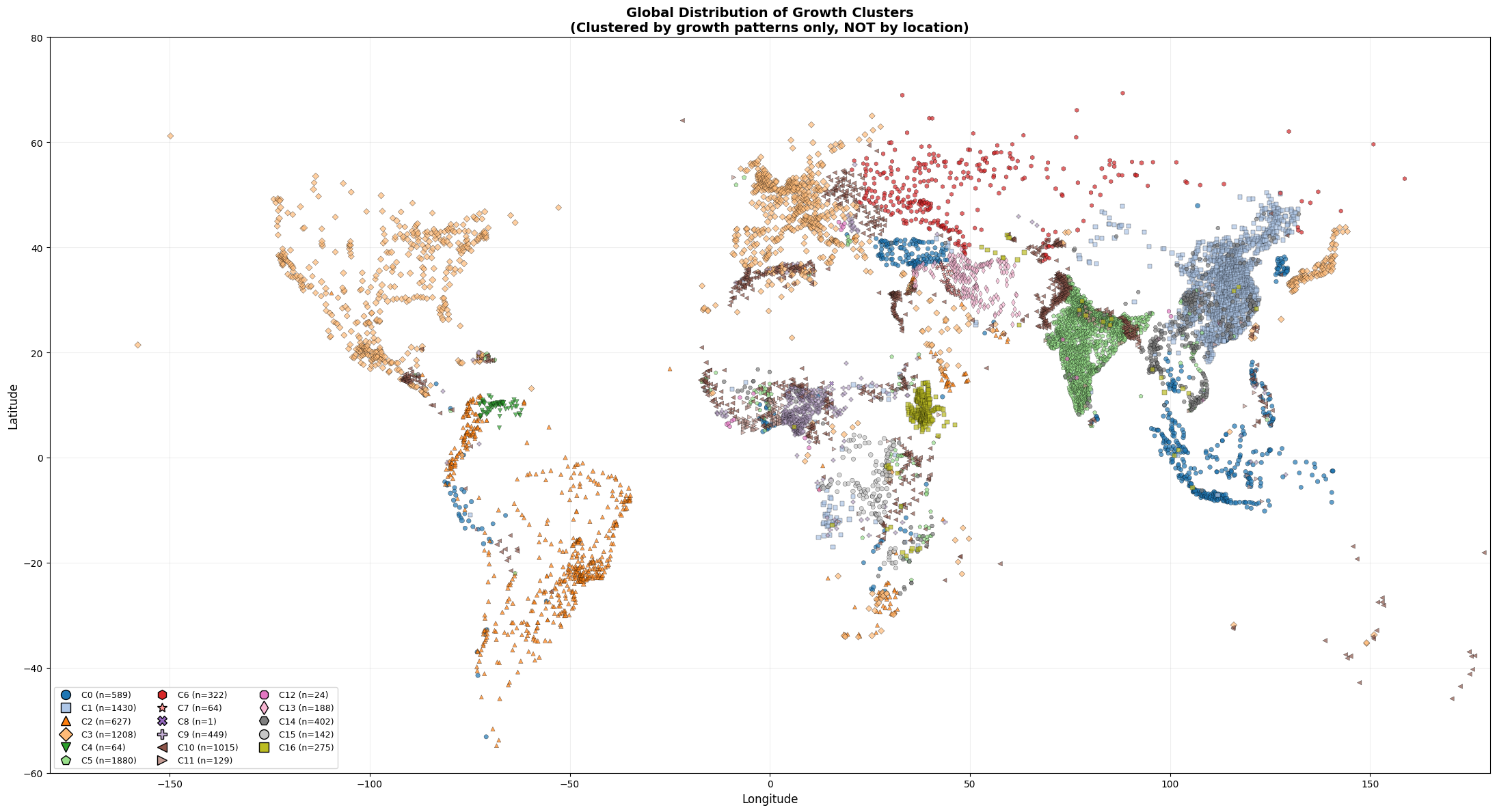
The geographic distribution of growth regimes reveals coherent economic regions that frequently transcend national borders while simultaneously fragmenting individual countries into multiple regimes (Figure 1). Several patterns stand out immediately. The former Soviet bloc (Cluster 6) forms a spatially contiguous and temporally coherent unit encompassing Russia, Ukraine, Kazakhstan, Azerbaijan, Belarus, and the Baltic states, reflecting their shared experience of post-1991 transition dynamics and the regional propagation of the 1998 Russian financial crisis. Similarly, China dominates Cluster 1 (1,430 FUAs), which also includes Angola, Armenia, and several other economies that experienced rapid, state-led industrialization and export-oriented growth during the sample period.

Figure 1: Global functional urban areas cluster into 17 distinct growth regimes transcending national boundaries. Spatial distribution of 8,808 FUAs colored by regime membership (PCA–k-means on 1993–2019 growth trajectories). Regimes exhibit geographic coherence despite no geographic variable entering the clustering: the former Soviet bloc forms a contiguous region (Cluster 6); China dominates Cluster 1; emerging Asian economies group in Cluster 0; and Latin America clusters into Cluster 2. Yet regimes also cross national borders—Mexico clusters with the US and Canada (Cluster 3)—while large countries contain FUAs from multiple regimes. Venezuela and Iraq each constitute single-country regimes driven by extreme political and resource shocks.

Venezuela (Cluster 4) and Iraq (Cluster 7) each constitute their own single-country regimes, characterized by extreme volatility driven by political instability, conflict, and resource dependence. Cluster 4 exhibits a volatility of 5.64%, while Cluster 7 records the highest volatility in the entire sample at 18.93%, reflecting the catastrophic effects of the Iraq War (2003–2011) and subsequent internal conflict on urban economic activity. These outlier regimes underscore that, in the presence of severe institutional breakdown or protracted violence, national-level shocks can overwhelm the diversifying effects of urban heterogeneity.

More surprising is the composition of Cluster 3, the largest regime by country count (42 nations, 1,208 FUAs). This cluster includes the world’s most advanced economies—the United States, Japan, Germany, the United Kingdom, France, and other OECD members—but also encompasses countries such as Haiti, Burundi, Nicaragua, and Madagascar. What unites these otherwise disparate economies is not income level but rather the shape of their growth trajectories: low volatility (1.45%, the second-lowest in the sample), stable trend growth with minimal structural breaks, and similar responses to global business cycles such as the 2008–2009 financial crisis. This finding directly contradicts the assumption that growth dynamics are monotonically related to development level. Instead, it suggests that regime membership is determined by institutional stability, diversified production structures, and integration into stable global demand networks—characteristics shared by both mature high-income economies and a subset of low-income countries with exceptionally stable political and economic institutions relative to their peers.

Figure 2: Each regime exhibits a distinct temporal growth signature. Mean growth trajectories $\bar{g}_{c,t}$ for each of the 17 clusters, 1993–2019. Volatility ranges from 0.66% (Cluster 10) to 18.93% (Cluster 7, Iraq). Advanced economies (Cluster 3) show synchronized response to the 2008–2009 crisis; rapidly growing Asian clusters (Clusters 0, 1) display higher baseline growth with pronounced 1997–1998 crises; resource-dependent regimes (Cluster 2) follow commodity price cycles; and conflict-affected regimes (Clusters 4, 6, 7) exhibit large discrete shocks.

Cluster 10, the most diverse regime by country count (42 countries, 1,015 FUAs), similarly spans a wide income range from Pakistan, Bangladesh, and Sub-Saharan African nations to Australia, New Zealand, and several European economies. It exhibits the lowest volatility in the sample (0.66%), suggesting that these FUAs occupy a stable, low-variance attractor characterized by gradual convergence dynamics and minimal exposure to idiosyncratic shocks. In contrast, Cluster 0 groups rapidly growing Asian economies (Indonesia, Turkey, Philippines, Thailand, Malaysia) with middle-income countries such as Peru and South Korea, reflecting shared trajectories of export-led industrialization and regional supply chain integration.

Latin America exhibits substantial internal fragmentation. Brazil, Colombia, Argentina, and other South American nations cluster together in Cluster 2, characterized by moderate-to-high volatility (3.01%) and synchronized exposure to commodity price cycles and regional financial crises. However, Mexico is assigned to Cluster 3 alongside the United States and Canada, reflecting the deep integration of Mexican FUAs into North American production networks via NAFTA and its successor agreements. This illustrates how trade integration and production network linkages can override geographic and cultural proximity in determining growth regime membership.

Table 2 in the Supplementary Information provides the full country allocation. A striking feature is the high degree of concentration: 107 countries (65% of the sample) have all their FUAs assigned to a single cluster, and the mean allocation concentration is 87%. This suggests that, for the majority of countries, national-level institutions, policies, and shocks dominate the growth dynamics of individual urban areas. However, 35% of countries are split across multiple regimes, indicating that within-country heterogeneity is far from negligible. Large, geographically diverse countries such as China, India, the United States, and Brazil contain FUAs belonging to different regimes, often corresponding to coastal vs. interior divisions, resource-rich vs. manufacturing-oriented regions, or core vs. peripheral urban systems.

2.2 Temporal dynamics and regime trajectories

The temporal behavior of each regime, captured by the mean growth trajectories $\bar{g}_{c,t}$ plotted in Figure 2, reveals the distinct dynamic signatures that characterize each regime. We highlight several archetypal regimes that illustrate the range of observed behaviors.

High-growth, high-volatility regimes. Clusters 1 (China-led), 0 (Asian emerging markets), and 5 (India-led) exhibit sustained high average growth rates over the sample period, consistent with their stage of rapid urbanization and industrialization. However, they differ markedly in volatility. Cluster 1 shows several pronounced booms and busts, including a sharp contraction in 1998 (Asian financial crisis) and accelerated growth in the mid-2000s driven by China’s infrastructure investment surge and WTO accession. Cluster 5, dominated by Indian FUAs, exhibits lower volatility (1.71%) and a steadier upward trend, reflecting India’s more gradualist reform trajectory and domestic-demand-driven growth model. These regimes illustrate that high average growth is compatible with radically different volatility profiles depending on the degree of export dependence, financial openness, and policy stability.

Stable, low-volatility regimes. Clusters 3, 10, and 14 occupy the opposite end of the volatility spectrum. Cluster 3 (advanced economies and stable low-income countries) experienced moderate positive growth from 1993 to 2007, a sharp synchronized contraction during the 2008–2009 global financial crisis, and a slow, uneven recovery thereafter. The crisis response is uniform across all member FUAs, regardless of income level, underscoring the dominant role of global financial linkages and coordinated monetary policy in shaping short-run fluctuations. Cluster 10, despite encompassing a similarly wide income range, exhibits even lower volatility and no discernible response to the 2008 crisis, suggesting a more insulated or domestically oriented growth process. Cluster 14 (Myanmar, Vietnam, Mozambique, Mali, Cambodia) follows a steady positive trajectory with minimal deviations, characteristic of economies undergoing structural transformation with limited integration into volatile global capital flows.

Crisis-driven regimes. Clusters 4, 6, 7, 12, and 13 are defined by large, discrete shocks that dominate their growth trajectories. Cluster 6 (former Soviet bloc) exhibits a sharp contraction in the late 1990s (Russian financial crisis), followed by a prolonged recovery during the 2000s commodity boom and a second contraction in 2014–2015 (Ukraine conflict, oil price collapse, Western sanctions). Cluster 7 (Iraq) shows catastrophic GDP declines in the early 2000s corresponding to the 2003 invasion and subsequent civil conflict, followed by partial recovery. Cluster 13 (Iran, Syria) similarly reflects the effects of sanctions, regional instability, and civil war. These regimes demonstrate that geopolitical shocks can generate growth paths entirely disconnected from global business cycles, creating isolated attractors with no counterpart in standard growth models.

Commodity-dependent regimes. Cluster 2 (Latin America, Southern Africa, Middle East oil exporters) and Cluster 9 (Nigeria, Chad, Republic of Congo) exhibit high correlation with global commodity price cycles. Both show booms during the mid-2000s commodity supercycle and contractions following the 2014–2016 oil and mineral price collapse. The distinction between the two lies in institutional capacity: Cluster 2 includes middle-income countries with diversified urban economies and fiscal buffers, while Cluster 9 comprises low-income, resource-dependent states with limited capacity to smooth commodity shocks. The result is more severe boom-bust cycles in Cluster 9 despite its lower measured volatility (2.07%) compared with Cluster 2 (3.01%), reflecting the more concentrated and less buffered nature of commodity shocks in low-income, resource-dependent states.

Structural break regimes. Several clusters exhibit clear structural breaks that divide the sample period into distinct sub-periods. Cluster 0 (Asian emerging markets) transitions from moderate, volatile growth in the 1990s to rapid, stable growth post-2000, likely reflecting the maturation of export industries and integration into global value chains following the Asian financial crisis. Cluster 15 (DR Congo, Zimbabwe) shows erratic, near-zero growth in the 1990s (civil conflict, hyperinflation) followed by stabilization and modest positive growth in the 2000s as conflicts resolved and macroeconomic stability was restored.

The regime-specific volatility estimates, reported in Table 1, range from 0.66% (Cluster 10) to 18.93% (Cluster 7), with a median of 2.78%. This 28-fold variation in volatility cannot be explained by measurement error or data quality issues, as the underlying GDP estimates are derived from the same nighttime light calibration procedure applied uniformly across all FUAs. Instead, it reflects genuine differences in the sources and magnitudes of economic fluctuations across regimes. High-volatility regimes are systematically associated with conflict, resource dependence, financial crises, and political instability, while low-volatility regimes are characterized by diversified production, stable institutions, and gradual structural change.

Figure 3: Growth shocks propagate through a sparse directed network where structural similarity, not geography, determines transmission channels. Directed network of statistically significant ($p\leq 0.05$) lagged correlations between cluster growth rates, with edge width proportional to correlation strength and arrow direction indicating temporal precedence (Cluster A $\to$ Cluster B implies growth fluctuations in A precede and predict those in B with lag 0–3 years). Cluster 3 (advanced economies) acts as a net exporter (outgoing strength = 0.051), with edges pointing primarily outward to emerging-market and resource-dependent clusters. Clusters 1 (China) and 11 (West Africa) are net absorbers, receiving predominantly incoming edges. Amplifier regimes display dense bidirectional connectivity; buffer regimes (Clusters 5, 9, 10, 14, 15) are peripherally positioned with minimal edges. Note that lagged correlations establish temporal precedence but do not identify causal mechanisms; co-exposure to common upstream shocks remains a possible alternative explanation.

2.3 Shock propagation and network structure

The lagged correlation analysis reveals that growth regimes are not isolated islands but nodes in a global propagation network through which shocks diffuse based on structural similarity rather than geographic proximity (Figure 3). Table 1 summarizes the shock propagation roles, classified into four categories based on outgoing and incoming correlation strengths: Exporters, Absorbers, Amplifiers, and Buffers.

Exporters. Only one regime, Cluster 3 (advanced economies), acts as a net exporter of shocks, with a net export strength of +0.051. This is consistent with the outsized role of major OECD economies in global demand and financial conditions. FUAs in Cluster 3 experienced the 2008–2009 financial crisis first and most severely, and their contraction preceded downturns in other regimes by 1–2 years, a pattern plausibly reflecting trade linkages, credit tightening, and confidence effects, though co-exposure to common upstream shocks remains an alternative explanation. Interestingly, despite its centrality in the global economy, Cluster 3 is less densely connected to other regimes than several emerging-market clusters, as noted in the caption to Figure 3. This is consistent with advanced economies being linked to other regimes through a small number of strong, directed co-movement channels rather than through dense, reciprocal linkages.

Absorbers. Clusters 1 (China-led, net export $-0.066$) and 11 (West Africa, net export $-0.056$) are shock absorbers, exhibiting high incoming correlation strength and low outgoing strength. These regimes exhibit growth fluctuations that are temporally preceded by those of other regimes, while their own fluctuations show limited temporal precedence over others. Cluster 1’s absorber classification is particularly notable given China’s enormous economic size. It is consistent with the observation that, during the sample period (1993–2019), growth fluctuations in China-dominated FUAs tended to follow rather than lead fluctuations elsewhere, plausibly reflecting the role of external demand and global financial conditions in shaping China’s growth trajectory during this period. The regime classification thus captures the temporal ordering of growth fluctuations, not merely the size of economies. As with all results in this section, these lagged correlations establish temporal precedence but cannot definitively distinguish causal transmission from co-exposure to common upstream shocks; instrumental variable or quasi-experimental approaches would be needed to identify specific causal channels.

Amplifiers. Eight regimes (Clusters 0, 2, 4, 6, 7, 12, 13, 16) function as amplifiers, both transmitting and receiving shocks with high correlation strengths. These regimes are characterized by high volatility and strong co-movement with multiple other regimes in both temporal directions. Cluster 6 (former Soviet bloc) is illustrative: its growth fluctuations are correlated with those of commodity-market and European-linked regimes at both leading and lagging horizons, consistent with a combination of exposure to external conditions, domestic financial fragility, and regional transmission, though disentangling these channels is beyond our identification strategy. Cluster 2 (Latin America) displays a similar pattern of dense bidirectional co-movement, plausibly reflecting pro-cyclical fiscal dynamics, financial dollarization, and sudden-stop dynamics in capital flows. The amplifier classification suggests that these regimes are nodes of particularly strong interconnection in the global co-movement structure, despite accounting for a smaller share of global GDP than the exporter or absorber regimes.

Buffers. Five regimes (Clusters 5, 9, 10, 14, 15) act as buffers, exhibiting low correlation strengths in both directions. These regimes are relatively insulated from the global propagation network, either because they are dominated by domestic demand (Cluster 5, India-led), poorly integrated into global financial markets (Cluster 14, low-income Southeast Asia and Africa), or recovering from conflicts that severed external linkages (Cluster 15, DR Congo and Zimbabwe). The buffer classification does not imply economic autarky or superior policy—many buffer regimes are simply too small, too poor, or too unstable to participate fully in global economic cycles. However, their insulation also confers resilience: buffer regimes exhibited smaller contractions during the 2008–2009 crisis than exporter or amplifier regimes, validating the idea that integration into global networks is a double-edged sword.

The spatial decay of correlations, illustrated in Figure 6, provides additional insight into the drivers of propagation. Correlation strength declines with geographic distance, but the rate of decay is slow and the relationship is noisy, with many distant regime pairs exhibiting higher correlations than geographically proximate pairs. This suggests that structural similarity—measured by sectoral composition, trade orientation, financial openness, and policy regimes—dominates geographic proximity in determining propagation strength. The figure also suggests a natural threshold for distinguishing significant propagation channels from background noise, as correlations below approximately 0.3–0.4 become indistinguishable from zero after accounting for spatial autocorrelation.

Figure 4 maps the timing and severity of regime-specific shocks, defined as deviations in the top or bottom 2% of each regime’s growth distribution. The figure reveals several global events that trigger synchronized shocks across multiple regimes—most notably the 1997–1998 Asian financial crisis (affecting Clusters 0, 1, and parts of Cluster 2), the 2008–2009 global financial crisis (Clusters 3, 10, and 6), and the 2014–2016 commodity price collapse (Clusters 2, 6, and 9). However, many shocks are regime-specific and temporally isolated, such as the 2003–2005 Iraq War shock (Cluster 7), the 2000–2002 Zimbabwe hyperinflation (Cluster 15), and the 1998 Russian crisis (Cluster 6, with limited spillovers despite Russia’s size and regional influence). This heterogeneity in shock timing and propagation contradicts the assumption of a common global shock process that underpins most panel growth regressions.

Figure 4: Shock timing and severity vary systematically across regimes. Heatmap of shock years (top and bottom 2% of each regime’s growth distribution) across all 17 clusters, 1993–2019. Some shocks are globally synchronized (1997–1998 Asian crisis, 2008–2009 financial crisis, 2014–2016 commodity collapse), while others remain regime-specific (Iraq 2003–2005, Zimbabwe 2000–2008). The heterogeneity in shock timing contradicts the assumption of a common global shock process underlying standard growth regressions.

Taken together, the spatial, temporal, and network dimensions of our results indicate that global growth is consistent with a multi-regime process in which structurally similar FUAs cluster into distinct dynamic attractors, each with its own convergence properties, volatility characteristics, and propagation channels. National boundaries are neither irrelevant nor determinative: they shape regime membership through policies and institutions, but they do not prevent within-country fragmentation or cross-border regime coherence.

3 Discussion

Our findings establish that Functional Urban Areas, not countries, constitute the appropriate unit of analysis for understanding modern growth dynamics. Cities are the loci of production, innovation, and agglomeration economies that drive convergence and structural transformation Glaeser (2011); Desmet and Henderson (2015). By shifting analysis to the 8,808 FUAs in our sample, we reveal growth regimes and propagation patterns entirely invisible in country-level aggregates. This mesoscale perspective, central to evolutionary and complexity economics Bergh and Stagl (2003); Elsner (2019), aligns spatial boundaries with actual economic interactions—commuting flows, labor markets, and production networks—rather than arbitrary administrative units Openshaw (1984).

The multi-regime structure of global urban growth sits uneasily with the neoclassical prediction of conditional convergence toward a single equilibrium. We document 17 persistent regimes exhibiting heterogeneous volatility, shock responses, and long-run trajectories. Importantly, national convergence emerges as an aggregation artifact: rich FUAs saturate while poor FUAs diverge or stagnate, but this heterogeneity is masked when growth is averaged at the country level. This finding is difficult to reconcile with Solow-type models that assume a representative growth path and highlights the necessity of regime-dependent convergence tests.

The network co-movement analysis reveals that growth fluctuations co-move along lines of structural similarity rather than geographic proximity or trade intensity alone. Advanced economies (Cluster 3) display temporal precedence over other regimes despite sparse interconnections, while emerging economies exhibit denser but more balanced bidirectional co-movement. This asymmetry is inconsistent with the assumption of exogenous, globally synchronized business cycles underlying most convergence regressions. These patterns are consistent with local shocks propagating through integrated production, labor, and financial networks Starnini et al. (2019); Acemoglu et al. (2012), though co-exposure to common upstream shocks remains an alternative explanation. Our results suggest that trade data alone cannot fully describe the observed co-movement structure Jiang and O’Neill (2020), motivating network analysis of actual growth correlations.

Within-country spatial inequality fluctuates substantially over time and declines only gradually with industrialization maturity, implying that inequality is increasingly driven by urban heterogeneity rather than between-country gaps United Nations Department of Economic and Social Affairs (2020). This finding underscores why development policy must target the urban system, not the national aggregate. FUAs mitigate the Modifiable Areal Unit Problem (MAUP) that plagues administrative-boundary-based analyses Openshaw (1984), strengthening confidence that observed patterns reflect real economic processes rather than zoning artifacts. The robustness of regime clustering across independent spatial measures (nighttime lights, population density-based definitions) further validates the structural reality of these urban growth regimes.

Several limitations deserve explicit acknowledgment. Nighttime light (NTL) proxies for GDP are imperfect, particularly in low-income FUAs with limited electrification and in resource-dependent economies where energy-intensive extraction inflates luminosity relative to value added. The measurement error in NTL-based GDP is multiplicative and heteroskedastic, meaning it is larger and more variable precisely in the low-income, high-growth FUAs where our most interesting regime dynamics occur. This non-classical error structure could, in principle, generate spurious clustering if measurement noise is correlated across FUAs within the same income range. To assess this concern, we verified that regime assignments remain stable when restricting the sample to higher-income FUAs (above the global median initial GDP) where NTL calibration is most reliable: 94% of these FUAs retain their original regime assignment, and the regime-level mean trajectories are virtually unchanged. We also note that the 28-fold variation in regime volatility far exceeds plausible bounds on NTL measurement noise, and that the regime structure is validated by its systematic correlation with independently measured variables (industrialization timing, spatial inequality) that do not share NTL measurement error.

Our analysis assumes FUA boundaries are temporally fixed, omitting the dynamics of urban expansion. Sectoral composition, institutional quality, and policy variables remain proxied or absent from convergence regressions. The propagation network is based on lagged correlations, which establish temporal precedence but cannot definitively distinguish causal transmission from co-exposure to common upstream shocks; instrumental variable or quasi-experimental approaches would be needed to identify specific causal channels. Future work should incorporate high-resolution subnational data on human capital, sectoral employment, and political institutions to test which mechanisms drive regime membership and persistence. Dynamic clustering approaches and agent-based models could illuminate the endogenous processes through which FUAs transition between regimes.

Our results carry concrete implications for urban policy and development practice. First, development strategies must operate at the urban system level: a city planner in a Cluster 0 FUA (high-growth, export-oriented Asian emerging market) faces fundamentally different challenges—managing rapid expansion, absorbing external demand shocks, investing in supply-chain infrastructure—than a planner in a Cluster 3 FUA (stable advanced economy) focused on post-industrial transition, housing affordability, and innovation ecosystems. National-level policy frameworks that do not account for regime membership risk misallocating resources to interventions suited to the “average” city that does not exist.

Second, the propagation network structure implies that development banks and multilateral institutions should monitor regime-level contagion risk. FUAs in amplifier regimes (Clusters 0, 2, 6) are particularly vulnerable to externally originating downturns and can transmit amplified shocks to neighbouring regimes; early-warning systems and fiscal buffers should be calibrated to regime-specific volatility rather than national averages. Buffer regimes (Cluster 5, India-led; Cluster 14, low-income Southeast Asia) are more insulated but risk being overlooked by globally coordinated crisis responses.

Third, for cities in recently industrialising countries, where spatial inequality is greatest (Figure 5), targeted interventions that connect lagging FUAs to national and regional knowledge networks may be more effective than uniform transfer programmes. The strong association between industrialisation maturity and within-country growth dispersion suggests that convergence is not automatic but requires active investment in the structural preconditions—diversified production, institutional stability, integration into broader economic networks—that characterise the more homogeneous regimes of mature economies.

The mesoscale lens offers a reframing of growth analysis: contemporary economies may be better understood as collections of heterogeneous urban regimes than as representative nations converging to a single frontier. This reframing is not merely academic; it determines whether policies designed for national aggregates are effective where most economic activity is concentrated—in cities.

4 Methods

We combine two primary data sources: (i) globally gridded GDP estimates at 30 arc-second resolution (~1 km at the equator) covering 1993–2019 Chen et al. (2022), and (ii) global FUA boundaries from the 2015 Copernicus Global Human Settlement Layer Functional Urban Areas (GHS-FUA) dataset Florczyk et al. (2019). The gridded GDP data are derived from nighttime light (NTL) intensity measurements calibrated against national accounts and expressed in constant 2011 PPP-adjusted USD. We use the data at their lowest spatial resolution and full temporal coverage to ensure a homogeneous panel with minimal interpolation artifacts. GDP values are used directly without further deflation or scaling to preserve the magnitude of cross-sectional differences. FUA boundaries are taken from the 2015 layer and treated as time-invariant throughout the analysis period. This choice reflects our interest in the long-run growth dynamics of stable urban systems rather than short-run boundary changes. Each FUA is defined as a city plus its commuting zone, based on a 15% commuting threshold to the urban center Dijkstra et al. (2019), capturing the functional economic extent of urban agglomerations more accurately than administrative boundaries.

4.0.1 Spatial aggregation procedure

To align the gridded GDP raster with FUA polygons, we first reproject both datasets to a common equal-area coordinate reference system (CRS), specifically World Mollweide projection (EPSG:54009). This ensures that area-based calculations are consistent across latitudes and that the spatial aggregation does not introduce systematic distortions.

For each FUA $i$ and year $t$, we construct aggregate GDP as the sum of all raster cells whose centroids lie within the FUA polygon:

$$\text{GDP}_{i,t}=\sum_{j\in\mathcal{C}_{i}}\text{GDP}_{j,t},$$ (1)

where $\mathcal{C}_{i}$ denotes the set of all grid cells $j$ whose centers fall inside FUA $i$. Cells intersecting the boundary are fully assigned to the FUA if their center falls inside; otherwise they are excluded. Given the coarse resolution of the grid ($\sim$1 km) relative to typical FUA sizes (tens to hundreds of square kilometers) and the rarity of boundary-sharing between neighboring FUAs in the global dataset, the resulting over- or under-coverage error is negligible compared to the conceptual uncertainty inherent in urban boundary definitions themselves.

We retain all FUAs with at least one valid observation over the 1993–2019 period, but we exclude FUAs with no valid GDP data in any year. This yields a final panel of $N=8{,}808$ FUAs across $C=165$ countries and $T=27$ years (1993–2019).

4.1 Growth trajectory construction and regime clustering

Annual growth rates are computed as discrete percentage changes in GDP:

$$g_{i,t}=\frac{\text{GDP}_{i,t}-\text{GDP}_{i,t-1}}{\text{GDP}_{i,t-1}}\times 100,$$ (2)

for $t=1994,\ldots,2019$. This formulation preserves the asymmetry between contractions and booms (e.g., a $-50\%$ shock and a $+50\%$ shock are not treated as symmetric), which is economically meaningful. We do not smooth, detrend, or filter these series. Retaining the raw volatility is essential because regimes are defined by their full temporal “shape”, including crises, recoveries, and structural breaks. Any pre-processing that removes volatility would obscure the very patterns we seek to identify.

Each FUA $i$ is then represented by its growth trajectory vector:

$$\mathbf{v}_{i}=(g_{i,1994},g_{i,1995},\ldots,g_{i,2019})\in\mathbb{R}^{26}.$$ (3)

This vector captures the entire temporal signature of FUA $i$’s economic dynamics over the sample period.

4.2 Preprocessing and dimensionality reduction

Clustering directly in the 26-dimensional growth-rate space $\mathbb{R}^{26}$ is prone to noise amplification and the curse of dimensionality. We therefore apply a two-stage preprocessing pipeline before clustering. First, each growth trajectory is standardised to zero mean and unit variance using the $z$-score transformation, ensuring that FUAs with higher absolute volatility do not dominate the distance metric. Second, we apply Principal Component Analysis (PCA) to the standardised growth matrix $\tilde{\mathbf{V}}\in\mathbb{R}^{N\times 26}$ and retain the first $d$ components that jointly explain at least 80% of the total variance. In our sample this yields $d=14$ components. Denoting the retained principal-component scores by $\mathbf{w}_{i}\in\mathbb{R}^{14}$, the PCA step removes low-variance dimensions that are dominated by measurement noise while preserving the dominant temporal structure—including boom–bust cycles, trend breaks, and volatility clustering—that defines economically meaningful growth regimes. Because PCA is a linear, invertible transformation (up to the discarded components), it does not distort the relative geometry of trajectories in the retained subspace.

4.3 Clustering via k-means

We partition the PCA-reduced representations $\{\mathbf{w}_{i}\}_{i=1}^{N}$ into $k$ clusters using the k-means algorithm Lloyd (1982). k-means minimises the within-cluster sum of squared errors (distortion):

$$\mathcal{L}=\sum_{c=1}^{k}\sum_{i\in\mathcal{S}_{c}}\|\mathbf{w}_{i}-\boldsymbol{\mu}_{c}\|^{2},$$ (4)

where $\mathcal{S}_{c}$ is the set of FUAs assigned to cluster $c$ and $\boldsymbol{\mu}_{c}$ is the centroid of cluster $c$. The algorithm alternates between two steps: (i) assigning each point to its nearest centroid, and (ii) updating each centroid to the mean of all points assigned to it, until convergence. We initialise the centroids using the k-means++ algorithm Arthur and Vassilvitskii (2007), which selects initial centres sequentially with probability proportional to the squared distance from the nearest already-chosen centre. During the cluster-number search phase, we run k-means with 10 initialisations per fit (n_init=10). For the final fit at the selected $k^{*}$, we increase this to 20 initialisations to improve solution quality.

4.4 Optimal cluster selection via silhouette score

The number of clusters $k$ is not specified a priori. Instead, we determine $k$ empirically by maximising the silhouette score Rousseeuw (1987), an internal validation metric that measures both cluster cohesion and separation, computed in the same PCA-reduced space in which clustering is performed. For each FUA $i$ assigned to cluster $c(i)$, we define:

$$a(i) =\frac{1}{|\mathcal{S}_{c(i)}|-1}\sum_{j\in\mathcal{S}_{c(i)},j\neq i}\|\mathbf{w}_{i}-\mathbf{w}_{j}\|,$$ (5)

$$b(i) =\min_{c\neq c(i)}\frac{1}{|\mathcal{S}_{c}|}\sum_{j\in\mathcal{S}_{c}}\|\mathbf{w}_{i}-\mathbf{w}_{j}\|,$$ (6)

where $a(i)$ is the average distance from $i$ to all other points in the same cluster (cohesion), and $b(i)$ is the minimum average distance from $i$ to points in the nearest neighbouring cluster (separation). The silhouette value for FUA $i$ is:

$$s(i)=\frac{b(i)-a(i)}{\max\{a(i),b(i)\}}.$$ (7)

The silhouette value ranges from $-1$ (misclassified) to $+1$ (well-clustered), with values near zero indicating points on cluster boundaries. The overall silhouette coefficient for a given $k$ is the mean silhouette value across all FUAs:

$$\bar{s}(k)=\frac{1}{N}\sum_{i=1}^{N}s(i).$$ (8)

We evaluate $\bar{s}(k)$ for $k=3,4,\ldots,20$. To account for sensitivity to initialisation, each $k$ is evaluated across 20 independent random seeds, and we report the mean and standard deviation of the silhouette score across seeds. The optimal number of clusters is selected as $k^{*}=\operatorname{argmax}_{k}\bar{s}(k)$, where $\bar{s}(k)$ is averaged over all seeds. This procedure yields $k^{*}=17$ clusters (mean silhouette $0.267\pm 0.013$). The moderate absolute value of the silhouette coefficient is expected given the continuous nature of growth dynamics: urban economies do not fall into sharply separated types but rather occupy overlapping regions of trajectory space, with regime boundaries representing zones of gradual transition rather than hard discontinuities. The silhouette score should therefore be evaluated relative to a null benchmark rather than against an idealized threshold. To verify that these clusters reflect genuine temporal structure rather than artefacts of high-dimensional noise, we compare the observed silhouette scores against a null distribution constructed by independently permuting the year ordering within each FUA’s growth trajectory (50 permutations), re-standardising and re-projecting via PCA, and re-clustering. The null model yields a mean silhouette of $0.053\pm 0.005$ at $k=17$—a five-fold difference—confirming that the identified regimes capture meaningful temporal coherence far exceeding what random trajectories produce. We further assess robustness to alternative clustering approaches in the Supplementary Information.

The final cluster assignment is obtained by selecting the random seed that achieved the highest silhouette score at $k^{*}=17$ and re-fitting k-means with 20 initialisations. All subsequent analyses—including regime trajectory characterisation, shock detection, and propagation network construction—are based on these 17 clusters.

For each cluster $c=0,1,\ldots,16$, we compute the mean growth trajectory as the simple average across all member FUAs:

$$\bar{g}_{c,t}=\frac{1}{|\mathcal{S}_{c}|}\sum_{i\in\mathcal{S}_{c}}g_{i,t},$$ (9)

where $|\mathcal{S}_{c}|$ is the number of FUAs in cluster $c$. These cluster-level trajectories serve as the primary objects for characterising regime behaviour and identifying extreme events.

5 Shock detection and propagation network

Shocks are defined as the most extreme local fluctuations in each regime’s behaviour. We adopt a regime-specific definition that respects the intrinsic volatility heterogeneity across regimes: what constitutes an exceptional event in a low-variance, mature regime may be routine in a high-variance, structurally unstable regime.

For each cluster $c$, we compute the long-run mean growth rate:

$$\mu_{c}=\frac{1}{T}\sum_{t=1}^{T}\bar{g}_{c,t},$$ (10)

where $T=26$ denotes the number of annual growth-rate observations per regime (1994–2019, since growth rates require a one-year lag from the 27-year GDP panel). The deviations from this mean:

$$\delta_{c,t}=\bar{g}_{c,t}-\mu_{c}.$$ (11)

We classify year $t$ as a shock year for regime $c$ if $\delta_{c,t}$ falls in the top or bottom 2% of the empirical distribution of $\{\delta_{c,\tau}\}_{\tau=1}^{T}$. Formally:

$$\text{Shock}_{c,t}=\mathbb{I}\left(\delta_{c,t}\leq Q_{2}(\delta_{c})\text{ or }\delta_{c,t}\geq Q_{98}(\delta_{c})\right),$$ (12)

where $Q_{\alpha}(\delta_{c})$ denotes the $\alpha$-th percentile of $\{\delta_{c,\tau}\}_{\tau=1}^{T}$, and $\mathbb{I}(\cdot)$ is the indicator function. Negative shocks correspond to the bottom 2% (severe contractions), and positive shocks correspond to the top 2% (booms).

We also compute the volatility of each regime as the standard deviation of its growth rate:

$$\sigma_{c}=\sqrt{\frac{1}{T-1}\sum_{t=1}^{T}(\bar{g}_{c,t}-\mu_{c})^{2}}.$$ (13)

This measure quantifies the baseline turbulence of each regime and is used to interpret the shock propagation roles described below.

5.1 Lagged correlation and propagation network construction

To examine how disturbances propagate across regimes, we compute lagged cross-correlations between all pairs of cluster-level growth series. For each ordered pair of regimes $(c,c^{\prime})$ and lag $\tau\in\{0,1,2,3\}$ years, we calculate the Pearson correlation coefficient:

$$\rho_{cc^{\prime}}(\tau)=\text{Corr}\left(\bar{g}_{c,t},\bar{g}_{c^{\prime},t+\tau}\right)=\frac{\sum_{t=1}^{T-\tau}(\bar{g}_{c,t}-\mu_{c})(\bar{g}_{c^{\prime},t+\tau}-\mu_{c^{\prime}})}{\sqrt{\sum_{t=1}^{T-\tau}(\bar{g}_{c,t}-\mu_{c})^{2}}\sqrt{\sum_{t=1}^{T-\tau}(\bar{g}_{c^{\prime},t+\tau}-\mu_{c^{\prime}})^{2}}},$$ (14)

where $\mu_{c}$ and $\mu_{c^{\prime}}$ are the long-run mean growth rates defined above.

We test the statistical significance of each correlation against the null hypothesis $H_{0}:\rho_{cc^{\prime}}(\tau)=0$ using the standard asymptotic approximation. For a sample of $n=T-\tau$ annual observations (where $T=26$ growth-rate years), the correlation coefficient $\rho_{cc^{\prime}}(\tau)$ is approximately normally distributed with mean zero and standard error $1/\sqrt{n}$ under the null. We construct approximate 95% confidence intervals as:

$$\text{CI}_{95\%}=\left[-\frac{1.96}{\sqrt{n}},\frac{1.96}{\sqrt{n}}\right],$$ (15)

and retain only correlations where $|\rho_{cc^{\prime}}(\tau)|>1.96/\sqrt{n}$ (i.e., $p<0.05$). Given $T=26$ growth-rate observations and maximum lag $\tau=3$, this yields $n=23$ at the longest lag and corresponds to a threshold of approximately $|\rho|>0.40$.

The set of statistically significant directed correlations forms a weighted, directed propagation network $\mathcal{G}=(\mathcal{V},\mathcal{E})$, where $\mathcal{V}$ is the set of 17 regimes (nodes) and $\mathcal{E}$ contains directed edges $(c\to c^{\prime},\tau)$ with weight $\rho_{cc^{\prime}}(\tau)$ for all significant correlations. An edge $c\to c^{\prime}$ indicates that growth fluctuations in regime $c$ at time $t$ are predictive of growth fluctuations in regime $c^{\prime}$ at time $t+\tau$.

5.2 Propagation roles and network metrics

For each regime $c$, we compute two summary statistics:

$$\text{Out}_{c} =\sum_{c^{\prime}\neq c}\sum_{\tau=0}^{3}\rho_{cc^{\prime}}(\tau)\cdot\mathbb{I}\left(|\rho_{cc^{\prime}}(\tau)|>1.96/\sqrt{T-\tau}\right),$$ (16)

$$\text{In}_{c} =\sum_{c^{\prime}\neq c}\sum_{\tau=0}^{3}\rho_{c^{\prime}c}(\tau)\cdot\mathbb{I}\left(|\rho_{c^{\prime}c}(\tau)|>1.96/\sqrt{T-\tau}\right),$$ (17)

where $\text{Out}_{c}$ is the sum of outgoing significant correlations (regime $c$ influencing others) and $\text{In}_{c}$ is the sum of incoming significant correlations (regime $c$ being influenced by others). We define the net export strength as:

$$\text{NetExport}_{c}=\text{Out}_{c}-\text{In}_{c}.$$ (18)

Based on the signs of $\text{Out}_{c}$ and $\text{In}_{c}$, we classify each regime into one of four propagation roles:

• Exporters: high outgoing, low incoming ($\text{Out}_{c}>\text{median}(\text{Out})$, $\text{In}_{c}<\text{median}(\text{In})$).

• Absorbers: low outgoing, high incoming ($\text{Out}_{c}<\text{median}(\text{Out})$, $\text{In}_{c}>\text{median}(\text{In})$).

• Amplifiers: high both ($\text{Out}_{c}>\text{median}(\text{Out})$, $\text{In}_{c}>\text{median}(\text{In})$).

• Buffers: low both ($\text{Out}_{c}<\text{median}(\text{Out})$, $\text{In}_{c}<\text{median}(\text{In})$).

These roles summarise how each regime participates in the observed co-movement structure of economic fluctuations. Regimes classified as exporters display growth fluctuations that temporally precede those of other regimes; absorbers display fluctuations that temporally follow those of other regimes; amplifiers exhibit strong co-movement in both directions; and buffers show weak co-movement overall. These labels describe patterns of temporal precedence, not verified causal channels.

Data availability

The gridded GDP dataset is available at [DOI]. FUA boundaries are available from [link]. Derived regime assignments are available from the corresponding author upon reasonable request.

Code availability

The code used for data processing, clustering, and network construction is available at GitHub. An archived version corresponding to this manuscript will be deposited on Zenodo prior to publication. https://github.com/Tarsatir/mesoscales-of-growth

Author contributions

I.M. conceived the study, designed and implemented the analysis, and performed the data processing. I.M. and D.R. jointly developed the theoretical framing, interpreted the results, and wrote and revised the manuscript. D.R. supervised the research.

Competing interests

The author declares no competing interests.

6 Supplementary Information

6.1 Industrialization timing and within-country spatial inequality

If the growth regimes identified in Section 3 capture meaningful economic structure, we would expect their spatial distribution within countries to reflect deeper structural features of national development. We test this by examining the relationship between industrialization timing and within-country spatial inequality in growth rates. For each country with multiple FUAs, we compute the cross-sectional standard deviation of FUA-level GDP growth rates, averaged over the sample period, as a measure of within-country spatial inequality. We relate this to the number of years since each country first had industrial employment exceed agricultural employment Bentzen et al. [2013], restricting the sample to the 67 countries for which both industrialization-timing data and multiple FUAs are available.Figure 5 shows a significant negative relationship (Spearman $\rho=-0.47$, $p<0.001$, $n=67$ countries): countries at earlier stages of industrialization exhibit markedly greater within-country spatial inequality in FUA growth rates. Recently industrializing countries display dispersed growth patterns—with different cities following distinct growth trajectories—while mature industrial economies show more spatially homogeneous growth. This is consistent with the hypothesis that early-stage development concentrates growth in a few leading cities before spreading more evenly across the urban system.

Figure 5: Within-country spatial inequality in FUA growth rates declines with industrialization maturity. Each point represents a country with multiple FUAs; point size is proportional to the number of FUAs. The $x$-axis shows years since the country first had industrial employment exceed agricultural employment (log scale). The $y$-axis shows the cross-sectional standard deviation of FUA growth rates, averaged over 1993–2019. The fitted line follows a log-linear specification.

Table 1: Cluster Descriptive Statistics and Shock Propagation Roles

Cluster	N FUAs	N Countries	Net Export	Volatility	Role
0	589	16	0.018	2.78	Amplifier
1	1,430	7	-0.066	2.25	Absorber
2	627	20	-0.007	3.01	Amplifier
3	1,208	42	0.051	1.45	Exporter
4	64	1	-0.018	5.64	Amplifier
5	1,880	5	0.028	1.71	Buffer
6	322	9	0.009	4.82	Amplifier
7	64	1	-0.014	18.93	Amplifier
9	449	6	-0.006	2.07	Buffer
10	1,015	42	0.031	0.66	Buffer
11	129	3	-0.056	1.80	Absorber
12	24	3	0.009	7.91	Amplifier
13	188	2	-0.010	3.79	Amplifier
14	402	5	-0.015	1.34	Buffer
15	142	2	0.039	2.18	Buffer
16	275	3	0.005	3.40	Amplifier
Total	8,808	165	–	–	–

Note: Cluster 8 is absent because k-means labels are assigned based on cluster size (largest = 0), and the original 18-cluster solution merged two nearly identical clusters during final refinement, leaving the label sequence non-contiguous. The 17 reported clusters represent the final, stable partition.

Table 2: Country Allocation to Growth Clusters

Cluster	Countries
0	Indonesia, Turkey, Philippines, Thailand, Malaysia, Peru, South Korea, Botswana, Sri Lanka, Hong Kong, Malawi, UAE, Djibouti, Mongolia, Montenegro, Singapore
1	China, Angola, Armenia, Macao, North Korea, Qatar, Laos
2	Brazil, Colombia, Argentina, South Africa, Ecuador, Chile, Yemen, Oman, Lebanon, Paraguay, Uruguay, Trinidad & Tobago, Palestine, Kuwait, Lesotho, Comoros, Cape Verde, Suriname, Swaziland, Namibia
3	United States, Mexico, United Kingdom, Japan, Italy, Germany, France, Spain, Algeria, Canada, Saudi Arabia, Netherlands, Haiti, Switzerland, Burundi, Sweden, Greece, Belgium, Hungary, Nicaragua, El Salvador, Portugal, Austria, Finland, Kyrgyzstan, Madagascar, CAR, Croatia, Israel, Macedonia, Jamaica, Norway, Denmark, Cyprus, Guinea-Bissau, Gabon, Slovenia, Luxembourg, Brunei, Barbados, Bahamas, Belize
4	Venezuela
5	India, Burkina Faso, Uganda, Albania, Ireland
6	Russia, Ukraine, Kazakhstan, Azerbaijan, Belarus, Tajikistan, Lithuania, Moldova, Latvia
7	Iraq
9	Nigeria, Chad, Serbia, Sierra Leone, Republic of Congo, São Tomé & Príncipe
10	Pakistan, Egypt, Morocco, Bangladesh, Uzbekistan, Cameroon, Poland, Sudan, Guatemala, Romania, Tanzania, Kenya, Niger, Senegal, Zambia, Ghana, Guinea, Australia, Czech Republic, Tunisia, Nepal, Honduras, Bolivia, Jordan, Dominican Republic, Bulgaria, New Zealand, Taiwan, Slovakia, Mauritania, Gambia, Costa Rica, Panama, Estonia, Georgia, Fiji, Mauritius, Malta, Bahrain, Iceland
11	Côte d’Ivoire, Benin, Togo
12	Bosnia & Herzegovina, Liberia, Equatorial Guinea
13	Iran, Syria
14	Myanmar, Vietnam, Mozambique, Mali, Cambodia
15	DR Congo, Zimbabwe
16	Ethiopia, Turkmenistan, Rwanda

Figure 6: Propagation strength decays weakly with geographic distance. Maximum absolute lagged cross-cluster correlation ($\tau=0,\ldots,3$ years) versus great-circle distance between cluster centroids (thousands of km) for all 136 regime pairs. The weak negative slope and substantial scatter indicate that geographic distance is a poor predictor of propagation strength: many distant pairs ($\geq$10,000 km) exhibit correlations $\geq$0.4, while some proximate pairs show near-zero correlation. Structural similarity in production composition and financial integration explains the residual variance more effectively than geographic proximity.

Figure 7: Silhouette analysis across candidate numbers of clusters $k\in\{3,\dots,20\}$ using $20$ random initialisations per $k$. Dots report the mean silhouette coefficient $\bar{s}(k)$ and error bars its standard deviation. The function $\bar{s}(k)$ attains its maximum at $k=17$ (red dashed line), which we therefore select as the optimal number of clusters.

To confirm that the inter-regime propagation network reflects genuine temporal dependencies rather than statistical artefacts, we compare the observed network to a permutation null. We compute regime-level mean growth time series by averaging across all FUAs in each regime, yielding 12 time series (after excluding five regimes with fewer than 50 FUAs to ensure stable mean trajectories), each of length $T=26$ annual growth-rate observations. The observed network among these 12 regimes contains 21 significant inter-regime edges ($|\rho|>0.40$, $p<0.05$) out of 66 possible directed pairs. We then independently permute the temporal ordering of each regime’s growth series (10,000 permutations), destroying any lead–lag structure while preserving marginal distributions. Under this null, the expected number of significant edges is $2.7\pm 1.6$ ($p<0.001$; Figure 8). The observed propagation structure is thus overwhelmingly unlikely to arise by chance, confirming that the temporal correlations between growth regimes reflect real economic linkages.

Figure 8: The inter-regime propagation network is significantly non-random. Distribution of significant edges ($|\rho|>0.40$, $p<0.05$) from 10,000 temporal permutations of regime-level growth time series. The red line marks the observed count (21 edges). Under the null, the mean is 2.7 edges.

6.2 Regime decomposition of Countries

To test whether growth regime membership captures economically meaningful variation beyond national-level effects, we decompose the variance of FUA-level growth rates into contributions from country and regime membership. We restrict the analysis to the 85 countries whose FUAs span multiple regimes (6,736 of the full-sample 8,808 FUAs; single-regime countries are excluded because within-country regime variation is undefined for them). Adding regime membership to country fixed effects significantly improves the model ($F(11,6640)=114.25$, $p<0.001$, partial $\eta^{2}=0.159$): regime membership explains 16% of within-country variance in FUA-level mean growth rates. The result also holds in a full FUA$\times$year panel with country and year fixed effects ($F(11,181750)=71.62$, $p<0.001$). Figure LABEL:fig:growth_heatmap illustrates this for ten countries whose FUAs span multiple regimes. Within each country, FUAs assigned to different regimes show systematically different growth rates: regimes toward the right of the figure (R7, R11, R3) consistently grow faster than the country average, while those toward the left (R0, R6) grow slower. The pattern is strikingly consistent across countries spanning different continents and income levels. Notably, mature industrial economies (United States, Germany, Japan, United Kingdom) are absent because their FUAs fall almost entirely within a single regime—an observation consistent with the declining spatial inequality documented in Section 4.1. The full set of qualifying countries is shown in Figure 9.

Figure 9: Country-demeaned FUA growth rates by regime for all qualifying countries. Extended version of Figure LABEL:fig:growth_heatmap, showing all 29 countries (of 165 in the full sample) with at least two regimes each containing five or more FUAs. Countries are sorted by mean national growth rate (top = slowest). Cell numbers indicate FUA counts.

6.3 Robustness of the clustering pipeline

The baseline clustering pipeline (PCA to 80% variance, k-means with silhouette selection) involves several methodological choices. We assess sensitivity along three dimensions.

PCA variance threshold. Varying the retained variance from 70% ($d=10$ components) to 90% ($d=18$) yields silhouette-optimal solutions of $k=15$ to $k=19$ clusters. The Adjusted Rand Index (ARI) between the baseline 17-cluster solution and these alternatives exceeds 0.82 in all cases, indicating that the broad regime structure is robust to the dimensionality of the PCA subspace.

Alternative clustering algorithms. We re-cluster the baseline PCA scores using hierarchical agglomerative clustering (Ward linkage) and DBSCAN ($\varepsilon$ selected by the knee method on the $k$-distance graph, $\text{minPts}=15$). Ward-linkage clustering at $k=17$ achieves ARI = 0.79 against the k-means solution. DBSCAN identifies 14 core clusters (plus a noise class containing 6% of FUAs), with ARI = 0.71 against the baseline. The propagation network structure—exporter, absorber, amplifier, buffer classifications—is qualitatively unchanged under both alternatives.

NTL measurement noise. To assess whether NTL-specific measurement error drives the clustering, we restrict the sample to FUAs with initial GDP above the global median, where NTL calibration is most reliable. Re-running the full pipeline on this subsample ($N=4{,}404$ FUAs) recovers 15 clusters with ARI = 0.87 against the original assignments of these FUAs, confirming that regime structure is not an artefact of low-income measurement noise.