Nodule-Aligned Latent Space Learning with LLM-Driven Multimodal Diffusion for Lung Nodule Progression Prediction

Abstract

Early diagnosis of lung cancer is challenging due to biological uncertainty and the limited understanding of the biological mechanisms driving nodule progression. To address this, we propose Nodule-Aligned Multimodal (Latent) Diffusion (NAMD), a novel framework that predicts lung nodule progression by generating 1-year follow-up nodule computed tomography images with baseline scans and the patient’s and nodule’s Electronic Health Record (EHR). NAMD introduces a nodule-aligned latent space, where distances between latents directly correspond to changes in nodule attributes, and utilizes an LLM-driven control mechanism to condition the diffusion backbone on patient data. On the National Lung Screening Trial (NLST) dataset, our method synthesizes follow-up nodule images that achieve an AUROC of 0.805 and an AUPRC of 0.346 for lung nodule malignancy prediction, significantly outperforming both baseline scans and state-of-the-art synthesis methods, while closely approaching the performance of real follow-up scans (AUROC: 0.819, AUPRC: 0.393). These results demonstrate that NAMD captures clinically relevant features of lung nodule progression, facilitating earlier and more accurate diagnosis.

1 Introduction

Early diagnosis is a cornerstone of modern medicine, enabling timely detection and intervention across a wide spectrum of diseases (WHO, 2025). Lung cancer, the leading cause of cancer-related mortality worldwide, carries an overall 5-year relative survival rate of only 22.9 $\%$. Prognosis improves substantially when the disease is detected early: the 5-year survival rate reaches 61.2 $\%$ for patients diagnosed with localized tumors, compared to just 7$\%$ for those presenting with advanced-stage disease (Institute, 2025). However, early detection remains particularly challenging in lung cancer, owing to an incomplete understanding of the biological mechanisms governing nodule progression and inherent biological uncertainty, which complicate the identification of early-stage lesions that will ultimately prove clinically consequential or lethal (Crosby et al., 2022). Consequently, only 15 $\%$ of lung cancer patients are currently diagnosed at an early stage (Kim ES, 2025). Low-dose computed tomography (LDCT) is widely employed for lung cancer screening in high-risk populations. In clinical practice, when LDCT findings are indeterminate, radiologists typically recommend follow-up imaging at six- to twelve-month intervals to monitor nodule progression. During this surveillance period, patients harboring malignant nodules may experience critical delays in definitive diagnosis and treatment initiation.

Over the past decade, with the emergence of artificial intelligence (AI) for the medical and healthcare applications, numerous machine learning (Gupta et al., 2024; Liu et al., 2024) and deep learning (Yu et al., 2025; Ardila et al., 2019; Wang et al., 2024b) models have been developed for lung cancer diagnosis, aiming to classify lung nodules as malignant or benign accurately. However, most existing approaches treat lung nodule diagnosis as a static, single time-point classification task. If future follow-up scans can be predicted from the baseline data, we can anticipate nodule progression and conduct early disease diagnosis.

Recent advances in controllable generative models have shown remarkable success in synthesizing high-fidelity images conditioned on semantic inputs (Labs, 2024; Tan et al., 2025). Prior studies (Wang et al., 2024a; Liu et al., 2025a; Wu et al., 2025; Chen et al., 2026) have explored generative models for disease progression prediction and reported promising results, offering a new avenue for achieving early diagnosis. However, clinical prognosis requires a level of precision beyond broad semantic conditioning (Tang et al., 2025; Liu et al., 2025b). Specifically, accurate lung nodule progression prediction demands fine-grained control over both nodule- and patient-specific factors, ensuring that generated outcomes adhere to clinical attributes rather than loosely defined semantics.

1.1 Our Contributions

In this study, we propose Nodule-Aligned Multimodal (Latent) Diffusion (NAMD) to model lung cancer progression by generating follow-up lung nodule images from baseline LDCT scans as well as patients’ and nodules’ EHR, with a focus on enabling fine-grained control over conditioning information. The main contributions of this work are summarized as follows:

• We propose a nodule-aligned latent space in which the variations of latent representation are enforced to align with meaningful changes in nodule attributes, thus enabling latent diffusion models (LDMs) to effectively capture the relationship between baseline and follow-up nodule images.

• We introduce an LLM-based diffusion control mechanism, where nodule- and patient-level metadata are converted into radiology report and embedded using a pretrained medical-focused large language model (LLM) with soft-prompt post-training adaptation. These embeddings are subsequently used as auxiliary context to guide the conditional diffusion generation with fine-grained control.

• We benchmarked NAMD through an extensive evaluation on the NLST dataset (Team, 2011). Our results demonstrate strong predictive performance, with synthesized one-year follow-up scans achieving diagnosis result significantly outperforms real baseline scans and existing state-of-the-art synthesis approaches, while nearly matching the diagnostic performance of real follow-up scans. These findings validate NAMD’s capability for accurate early disease diagnosis approximately one year in advance.

2 Background

2.1 Diffusion Models

A Denoising Diffusion Probabilistic Model (DDPM) (Sohl-Dickstein et al., 2015; Ho et al., 2020) is a deep generative model that has demonstrated its remarkable ability to synthesize high quality images. A diffusion model defines a forward process where Gaussian noise is progressively added to the original image $x_{0}\sim p_{\text{data}}$ over $T$ steps into noisy images $x_{t}$, where $t\in[T]$. It then learns a network $\epsilon_{\theta}$ that reverses this process, effectively mapping a standard normal distribution to the data distribution. Following work in Ho et al. (2020), we can train the network $\epsilon_{\theta}(x_{t},t)$ with the following:

$$\mathcal{L}(\theta)=\mathbb{E}_{\epsilon\sim\mathcal{N}(0,I),t,x_{t}}\left[\epsilon-\epsilon_{\theta}(x_{t},t)\right].$$ (1)

Although DDPM can generate high-quality images, its primary drawback lies in the substantial computational cost and prolonged inference time. To address this limitation, Denoising Diffusion Implicit Model (DDIM) (Song et al., 2021) introduces a formulation that yields the same training objective as DDPM but accelerates the sampling process by skipping certain timesteps without requiring retraining. Latent Diffusion Model (LDM) (Rombach et al., 2022) extend DDPM by applying the forward and reverse diffusion processes to lower-dimensional latent representations $z=E(x)$, encoded by a variational autoencoder (VAE) encoder $E$, rather than to the images $x$ directly. This substantially reduces computational cost while preserving image quality. In this work, we leverage the generative capabilities of latent diffusion models to model lung nodule progression for early malignancy prediction.

2.2 Latent Representation Learning

Learning compressed latent representations is foundational for modeling high-dimensional data. While standard frameworks, such as Variational Autoencoders (Kingma and Welling, 2014), effectively map data to lower-dimensional spaces, the resulting latent embeddings lack interpretable semantic structure. To address this, representation learning techniques are used to shape latent embeddings. In particular, supervised contrastive learning (Khosla et al., 2020) proposes to leverage ground truth information to pull representations of similar samples together while pushing dissimilar ones apart. Furthermore, recent work such as Representational Autoencoders (RAE) (Zheng et al., 2026) demonstrates that semantically rich latent spaces not only yield better reconstruction quality, but also superior generative qualities in downstream diffusion transformers. Given that clinical data often require fine-grain control and can be important for downstream clinical diagnosis, we draw upon these prior findings in representation learning to ensure that the latent space captures clinically relevant features necessary for progression modeling.

2.3 Parameter-Efficient LLM Adaptation

Large Language Models (LLMs) have demonstrated remarkable capabilities in clinical natural language processing, including the interpretation of medical texts and Electronic Health Records (EHR) (Sellergren et al., 2025). However, doing full parameter finetuning to adapt to specific tasks can be computationally expensive. To mitigate this, Parameter-Efficient Fine-tuning (PEFT) techniques have emerged to adapt models using only a fraction of its total parameters. Prominent techniques include Low-Rank Adaptation (LoRA) (Hu et al., 2022), which injects low rank decomposition matrices into linear layers while keeping original weights frozen. Another paradigm of PEFT is soft-prompt tuning (Lester et al., 2021), which directly acts on the input embedding space. Instead of training the model parameters, they prepend a set of learnable embedding vectors to the input sequence. This technique has shown great success in the medical domain; for example, Oh et al. (2024) uses soft prompt to allow LLMs to adapt clinical text into embeddings that cross-reference with image features.

3 Method

Figure 1: The overview of NAMD’s training process and latent space construction.

In this study, we aim to generate "virtual" one-year follow-up LDCT scans from baseline LDCT to improve early lung cancer diagnosis. We formulate this task as a conditional generative problem within a latent space, as illustrated in Figure 1. Adopting the Latent Diffusion Model (LDM) framework (Rombach et al., 2022), we first design a Nodule-Aligned Variational Auto-Encoder (VAE) to compress high-dimensional LDCT images into a compact latent representation. Within this latent space, an LLM-conditioned Diffusion Model characterizes lung nodule progression. The key challenge addressed by our model is enhancing controllability; while standard LDMs excel at broad semantic synthesis, lung cancer modeling necessitates fine-grained alignment with patient-specific EHR data and precise nodule morphology to ensure clinical utility.

3.1 Notations

Let $({\bm{X}}^{(1)},{\bm{X}}^{(2)},{\bm{e}},L)\sim\mathcal{D}$ denote a pair of longitudinal LDCT scans of the same lung nodule at two time points. Here, ${\bm{X}}^{(1)},{\bm{X}}^{(2)}\in\mathbb{R}^{H\times W}$ is a cropped, nodule-centered 2D image slice from the baseline and corresponding follow-up scan taken for the same patient after one year, respectively. ${\bm{e}}\in\mathbb{R}^{d}$ denotes the EHR vector containing nodule’s attributes ${\bm{f}}\in\mathbb{R}^{T}$ (e.g. diameter) corresponding to ${\bm{X}}^{(1)}$ and patient’s personal information ${\bm{p}}\in\mathbb{R}^{d-T}$ (e.g. family cancer history), and $L\in\{0,1\}$ indicates the prediction target label of nodule malignancy. Our target problem is to model a conditional distribution $p({\bm{X}}^{(2)}|{\bm{X}}^{(1)},{\bm{e}})$ for generating follow-up lung nodule image. Note that while fidelity to the ground truth ${\bm{X}}^{(2)}$ is important, the ultimate goal is downstream clinical prediction on $L$ based on the lung nodule progression prediction for achieving early diagnosis.

3.2 Nodule-Aligned Latent Space

To enable controllable generation of lung nodule progression along clinically meaningful attributes using latent diffusion models (LDMs), we introduce a nodule-aligned latent space learned via a distribution matching alignment objective. As illustrated in Figure 1, the goal is to structure the latent space such that distances between latent codes reflect similarities in nodule-level metadata.

3.2.1 Latent Alignment Loss.

Suppose $i,j\in[B]$ be the index of two arbitrary data samples, where $B\in\mathbb{Z}^{+}$ denotes the batch size. Let ${\bm{f}}_{i}\in\mathbb{R}^{T}$ be the feature vector containing the nodule’s metadata (e.g. diameter, margin, location). Let ${\bm{z}}_{i}=E({\bm{X}}_{i})$ be the latent embedding of the LDCT scan ${\bm{X}}_{i}$ encoded by the encoder $E$ of the VAE model. Denote the feature-space distance $({\bm{f}})$ and latent-space distance $({\bm{z}})$ between two data samples $(i,j)$ as

$$\ell_{ij}^{({\bm{f}})}=-\frac{||{\bm{f}}_{j}^{(n)}-{\bm{f}}_{i}^{(n)}||^{2}}{2\sigma_{{\bm{f}}}^{2}},\quad\ell_{ij}^{({\bm{z}})}=-\frac{||{\bm{z}}_{j}-{\bm{z}}_{i}||^{2}}{2\sigma_{{\bm{z}}}^{2}},$$ (2)

where $\sigma_{{\bm{f}}},\sigma_{{\bm{z}}}>0$ are hyperparameters to control the sharpness or sensitivity of the distance metric. Then, for each $i$, define the normalized rows as:

$$P_{ij}=\frac{\exp(\ell_{ij}^{({\bm{f}})})}{\sum_{k\neq i}\exp(\ell_{ik}^{({\bm{f}})})},\quad Q_{ij}=\frac{\exp(\ell_{ij}^{({\bm{z}})})}{\sum_{k\neq i}\exp(\ell_{ik}^{({\bm{z}})})},\quad P_{ii}=Q_{ii}=0.$$ (3)

We observe that $\sum_{j\neq i}P_{ij}=\sum_{j\neq i}Q_{ij}=1$. For each sample $i$, the row-wise normalization induces a distribution over relative similarities to other samples in the batch $B$. We then introduce the Kullback-Liebler(KL) Divergence loss $\mathcal{L}_{\text{align}}$ to align the two distributions:

$${\bm{P}}_{i}=\text{Categorical}(P_{i1},P_{i2},\dots,P_{iB});\quad{\bm{Q}}_{i}=\text{Categorical}(Q_{i1},Q_{i2},\dots,Q_{iB}),$$

$$\mathcal{L}_{\text{align}}=\frac{1}{B}\sum_{i=1}^{B}D_{\mathrm{KL}}({\bm{P}}_{i}\|{\bm{Q}}_{i})=\frac{1}{B}\sum_{i=1}^{B}\sum_{j\neq i}P_{ij}\log\frac{P_{ij}}{Q_{ij}}.$$ (4)

3.2.2 Predictive Representation Loss.

Inspired by similar implementations in DDL-CXR (Yao et al., 2024), we integrate representation learning with LDM training to ensure that the latent space captures clinical features relevant to the ultimate diagnostic task. Following the finding of RAE (Zheng et al., 2026), which suggests that semantically rich latent spaces lead to superior generative quality, we leverage ground-truth to structure the latent space by introducing a lightweight binary classification (benign v.s. malignant) objective $\mathcal{L}_{\text{pred}}$ on the latent ${\bm{z}}$. Specifically, we initialize a linear probe $h_{\theta}$ and optimize:

$$\mathcal{L}_{\text{pred}}=-L\log(h_{\theta}({\bm{z}}))-(1-L)\log(1-h_{\theta}({\bm{z}})).$$ (5)

3.2.3 Total Loss.

Building upon standard VAE training strategy (Kingma and Welling, 2014; Rombach et al., 2022), we incorporate a weighted combination of L1 Reconstruction Loss $\mathcal{L_{\text{rec}}}$, a KL divergence loss to regularize learned latent embeddings towards a standard normal distribution $\mathcal{L}_{\text{KL}}$, a perceptual loss $\mathcal{L}_{\text{LPIPS}}$ (Zhang et al., 2018) to balance perceptual semantics and pixel-wise accuracy, our proposed alignment loss $\mathcal{L}_{\text{align}}$ (Equation 4), and representation prediction loss $\mathcal{L}_{\text{pred}}$ (Equation 5):

$$\mathcal{L}_{\text{VAE}}(\theta)=\mathcal{L}_{\text{rec}}+\lambda_{KL}\mathcal{L}_{\text{KL}}+\lambda_{\text{LPIPS}}\mathcal{L}_{\text{LPIPS}}+\lambda_{\text{align}}\mathcal{L}_{\text{align}}+\lambda_{\text{pred}}\mathcal{L}_{\text{pred}},$$ (6)

where $\lambda_{KL},\lambda_{\text{LPIPS}},\lambda_{\text{align}},\lambda_{\text{pred}}$ denotes the hyperparameters of weighting for each loss.

3.3 LLM-Conditioned Latent Diffusion Model Generation

In the nodule-aligned latent space, temporal evolution of latent states is modeled using a latent diffusion generation process. As seen in Figure 1, we propose a multimodal latent diffusion model built on a U-Net backbone, with a pre-trained LLM serving as an auxiliary context encoder with information from EHR ${\bm{e}}$.

3.3.1 LLM Adaptation with Learnable Prompts.

We employ MedGemma 1.5 (4B) (Sellergren et al., 2025) as the foundation LLM, which is specifically designed for medical report understanding. To efficiently adapt the model under limited downstream data, we adopt a soft-prompt post-training adaptation paradigm (Oh et al., 2024), where a set of learnable prompts are trained to enable task-specific adaptation while keeping the original model weights frozen.

Given the EHR ${\bm{e}}\in\mathbb{R}^{d}$, we first convert it into a radiology report format (see Figure 1) and encode it into the LLM embedding space using the MedGemma tokenizer, yielding $\mathrm{emb}({\bm{e}})\in\mathbb{R}^{N\times D}$. We prepend $m$ sets of learnable prompt vectors $\mathbf{s}_{i,k}\in\mathbb{R}^{D}$ to the auxiliary context. Accordingly, the text prompt embeddings are constructed as:

$$\mathbf{c}_{j}=[\mathbf{s}_{j,1},\dots,\mathbf{s}_{j,n},\text{emb}({\bm{e}}_{j}),\texttt{<EOS>}],\quad\text{for }j\in\{1,\dots,m\}$$ (7)

The hidden state representation ${\bm{h}}_{j}^{\texttt{<EOS>}}$ corresponding to the last non-padding token position <EOS> token is extracted from the last hidden layer of the model as the auxiliary context embedding (i.e. $\mathbf{h}_{j}^{\texttt{<EOS>}}=\text{LLM}(\mathbf{c}_{j})_{[-1]}$). Because medgemma is a decoder-only LLM, which uses causal attention, the <EOS> token is the only token in the sequence that attends to all other tokens since it is the last token. Finally, we concatenate all ${\bm{h}}_{j}^{<EOS>}$ to form a sequence:

$$\mathbf{C}=[{\bm{h}}_{1}^{\texttt{<EOS>}},\dots,{\bm{h}}_{m}^{\texttt{<EOS>}}]$$ (8)

This embedding is then injected into our U-Net backbone at all layers via cross-attention to enable multi-modal conditioning of the diffusion process.

3.3.2 Latent Diffusion Model Training.

With the nodule-aligned VAE $E$ entirely frozen, the latent diffusion model operates entirely on the latent space. As Figure 1 shows, we adopt a two stage training strategy: an unconditional stage that learns the general latent distribution for lung LDCT images, and a conditional stage that learns to predict the follow-up LDCT image.

Unconditional Training

We first pre-train the denoising U-Net on unpaired latents to capture the marginal distribution of lung nodule appearances. Given a latent ${\bm{z}}=E({\bm{X}})$, the forward diffusion process adds Gaussian noise over $T$ timesteps: ${\bm{z}}_{t}=\sqrt{\bar{\alpha}_{t}}\,{\bm{z}}+\sqrt{1-\bar{\alpha}_{t}}\,\bm{\epsilon}$, where $\bm{\epsilon}\sim\mathcal{N}(\mathbf{0},\mathbf{I})$ and $\bar{\alpha}_{t}$ follows the standard noise schedule (Ho et al., 2020). The unconditional objective trains the network $\bm{\epsilon}_{\theta}$ to predict the added noise, with null prompt conditioning:

$$\mathcal{L}_{\text{uncond}}=\mathbb{E}_{{\bm{z}},\,\bm{\epsilon}\sim\mathcal{N}(\mathbf{0},\mathbf{I}),\,t}\Big[\big\|\bm{\epsilon}-\bm{\epsilon}_{\theta}({\bm{z}}_{t},\,t,\emptyset)\big\|^{2}\Big].$$ (9)

Conditional Training

Building on the pre-trained weights, we fine-tune the U-Net to model the conditional follow-up generation $p({\bm{z}}^{(2)}\mid{\bm{z}}^{(1)},{\bm{e}})$. Given a longitudinal pair $({\bm{X}}^{(1)},{\bm{X}}^{(2)})$, the baseline scan is encoded to ${\bm{z}}^{(1)}=E({\bm{X}}^{(1)})$ and the follow-up latent ${\bm{z}}^{(2)}=E({\bm{X}}^{(2)})$ serves as the diffusion target. The noisy follow-up latent ${\bm{z}}_{t}^{(2)}$ is constructed via the forward process on ${\bm{z}}^{(2)}$. The baseline latent ${\bm{z}}^{(1)}$ is channel-concatenated with ${\bm{z}}_{t}^{(2)}$ as input to the U-Net, while the LLM-derived context embedding $\mathbf{C}$ is injected via cross-attention. The conditional objective is:

$$\mathcal{L}_{\text{cond}}=\mathbb{E}_{{\bm{z}}^{(1)},{\bm{z}}^{(2)},\,\bm{\epsilon},\,t}\Big[\big\|\bm{\epsilon}-\bm{\epsilon}_{\theta}\!\big({\bm{z}}^{(1)},\,{\bm{z}}_{t}^{(2)},\,t,\,\mathbf{C}\big)\big\|^{2}\Big].$$ (10)

At inference, given a new baseline scan ${\bm{X}}^{(1)}$ and its associated EHR context, we sample ${\bm{z}}_{T}^{(2)}\sim\mathcal{N}(\mathbf{0},\mathbf{I})$ and iteratively denoise using $\bm{\epsilon}_{\theta}$ conditioned on ${\bm{z}}^{(1)}=E({\bm{X}}^{(1)})$ and $\mathbf{C}$ via DDIM (Song et al., 2021) with 50 steps, then decode the result via the VAE decoder $D$ to produce the predicted follow-up image $\hat{{\bm{X}}}^{(2)}=D(\hat{{\bm{z}}}^{(2)})$.

4 Experiments and Discussion

4.1 Experimental Setup

4.1.1 Dataset

We conduct experiments on the National Lung Screening Trial (NLST) dataset (Team, 2011), selecting 1,226 subjects with clinically defined indeterminate nodules and at least one longitudinal follow-up. For training and validation, we used 1,121 nodule baseline-follow-up image pairs (165 malignant, 611 benign) from 776 subjects. An independent hold-out test set comprised 450 pairs (53 malignant, 397 benign) from the remaining 450 subjects. All splits were performed at the patient level to prevent data leakage. Given the limited dataset size, NAMD utilizes pretrained StableDiffusion-1.5 weights (Rombach et al., 2022) and fine-tunes both the VAE and UNet backbones.

4.1.2 Evaluation Metrics

During evaluation, NAMD takes baseline LDCT images as conditions to generate follow-up nodule embeddings and images. To evaluate downstream diagnosis performance, we use a pre-trained ViT-based binary classification model to calculate the AUROC and AUPRC score. Note that this ViT model may underperformed compared to previously reported methods specifically tailored for lung nodule diagnosis, as we intend to use a standard architecture without task-specific adaptation. Its role is not to maximize diagnostic accuracy, but to provide a neutral evaluation framework for assessing NAMD’s ability to generate “virtual” follow-up nodules, while minimizing bias from highly specialized classifiers. We also use the FID and LPIPS (Zhang et al., 2018) to quantify distribution realism and perceptual similarity of the generated images compared to the real follow-up LDCT scan.

Due to the inherent stochasticity in diffusion models, generated images will be slightly different with different initial noise. To address this, we perform $K$ independent runs with different random seed and compute evaluation metrics for each run, then report the mean and standard deviation in Table 1. Empirically, we find $K=20$ to work well, as the variance in prediction probabilities stabilizes after more than 20 runs (Appendix D).

4.1.3 Compared Baseline Methods

We compare our method with several representative deterministic and stochastic generation approaches. We finetune from pretrained weights for SD1.5 (Rombach et al., 2022) and Flux (Labs, 2024). We evaluate against McWGAN (Wang et al., 2024a) and CorrFlowNet (Wu et al., 2025) which target the same progression prediction task we do. Because DDL-CXR (Yao et al., 2024) and ImageFlowNet (SDE) (Liu et al., 2025a) were originally developed for domains distinct from lung LDCT scans and utilize specialized architectures, we trained these models from scratch following their original implementations.

4.2 Main Results

Table 1: Comparison of methods and results from ablation study in terms of image quality metrics and diagnosis performance (AUROC and AUPRC). For stochastic methods, mean and standard deviation are calculated across 20 different samples from NAMD. Bold indicates best; underline indicates second best.

	Image Quality Metrics		Diagnosis Performance
Method	LPIPS $\downarrow$	FID $\downarrow$	AUROC $\uparrow$	AUPRC $\uparrow$
Real Image Baselines
Real baseline LDCT	-	-	0.742	0.263
Real follow-up LDCT	-	-	0.819	0.393
Deterministic Methods
McWGAN (Wang et al., 2024a)	0.364	80.443	0.763	0.307
CorrFlowNet (ODE) (Wu et al., 2025)	0.202	91.695	0.779	0.318
Stochastic Methods
SD1.5 (Rombach et al., 2022)	0.207 $\pm$ 0.003	97.550 $\pm$ 1.140	0.701 $\pm$ 0.031	0.245 $\pm$ 0.032
Flux (Rectified Flow) (Labs, 2024)	0.248 $\pm$ 0.002	95.843 $\pm$ 1.162	0.668 $\pm$ 0.030	0.227 $\pm$ 0.034
DDL-CXR (Yao et al., 2024)	0.235 $\pm$ 0.004	122.410 $\pm$ 2.409	0.701 $\pm$ 0.026	0.237 $\pm$ 0.030
ImageFlowNet (SDE) (Liu et al., 2025a)	0.362 $\pm$ 0.001	217.706 $\pm$ 1.051	0.782 $\pm$ 0.014	0.339 $\pm$ 0.022
CorrFlowNet (SDE) (Wu et al., 2025)	0.202 $\pm$ 0.001	88.560 $\pm$ 0.231	0.776 $\pm$ 0.004	0.321 $\pm$ 0.011
NAMD (Ours)	0.220 $\pm$ 0.001	83.060 $\pm$ 0.699	0.805 $\pm$ 0.018	0.346 $\pm$ 0.028
NAMD (w/o $\mathcal{L}_{\text{align}}$)	0.205 $\pm$ 0.002	101.301 $\pm$ 1.108	0.765 $\pm$ 0.017	0.305 $\pm$ 0.031

4.2.1 Early Diagnostic Performance.

As demonstrated in Table 1, our NAMD model substantial improves diagnostic performance by predicting follow-up nodules from baseline data. The resulting diagnosis model achieved a test AUROC of $0.805\pm 0.018$ and an AUPRC of $0.346\pm 0.028$ when using NAMD-generated follow-up nodule images in settings where only real baseline information is available. This represents a substantial gain over models using real baseline images (AUROC: $0.742$) and approaches the performance of models based on actual follow-up nodules (AUROC: $0.819$), effectively bridging the gap between baseline and future clinical data and suggest that NAMD effectively synthesizes follow-up images that preserve clinically relevant features for malignancy assessment. Moreover, when compared with baseline models, as shown in Table 1, our method outperforms all baseline approaches in both AUROC and AUPRC. Moreover, our NAMD achieves LPIPS and FID scores comparable to the best baselines.

4.2.2 Ablation Study.

Figure 2: t-SNE projection of the learned latent space. Left: Latent space learned by NAMD with alignment loss. Right: Latent space without the alignment loss.

We provide visualizations of the learned latent space in Figure 2 over the test set using t-SNE (van der Maaten and Hinton, 2008). NAMD constructs a latent space with structure as seen in Figure 2 left: nodules with shorter diameters (dark purple) at the top transitions to nodules with increasingly longer diameters. This spatial distribution suggests that the NAMD autoencoder has successfully captured nodule diameter as an important feature in its representation. In contrast, a VAE that is not nodule-aligned (Figure 2 right) results in a more entangled representation space.

To further assess the contribution of the nodule-aligned latent space, we also conducted an ablation study as summarized in the last two rows of Table 1. Specifically, when the alignment and prediction loss are omitted, AUROC and AUPRC drop from 0.805 to 0.765 and from 0.346 to 0.305 respectively. FID also worsens from 83.06 to 101.301, indicating a decrease in distribution similarity. While the unaligned variant achieves slightly improved LPIPS scores, this does not translate to improved diagnostic ability, indicating that structuring the latent space helps with capturing clinically meaningful nodule attributes.

4.3 Prediction Variance

Figure 3: Analysis of prediction variance and generated images. Left top: Prediction error vs. predictive variance. Left bottom: Predictive variance by true label. Right: NAMD-generated examples for confidently correct, unsure, and confidently incorrect predictions, showing one benign ($L=0$) and one malignant ($L=1$) case each. Pixel-wise variance and mean error maps are across 20 runs.

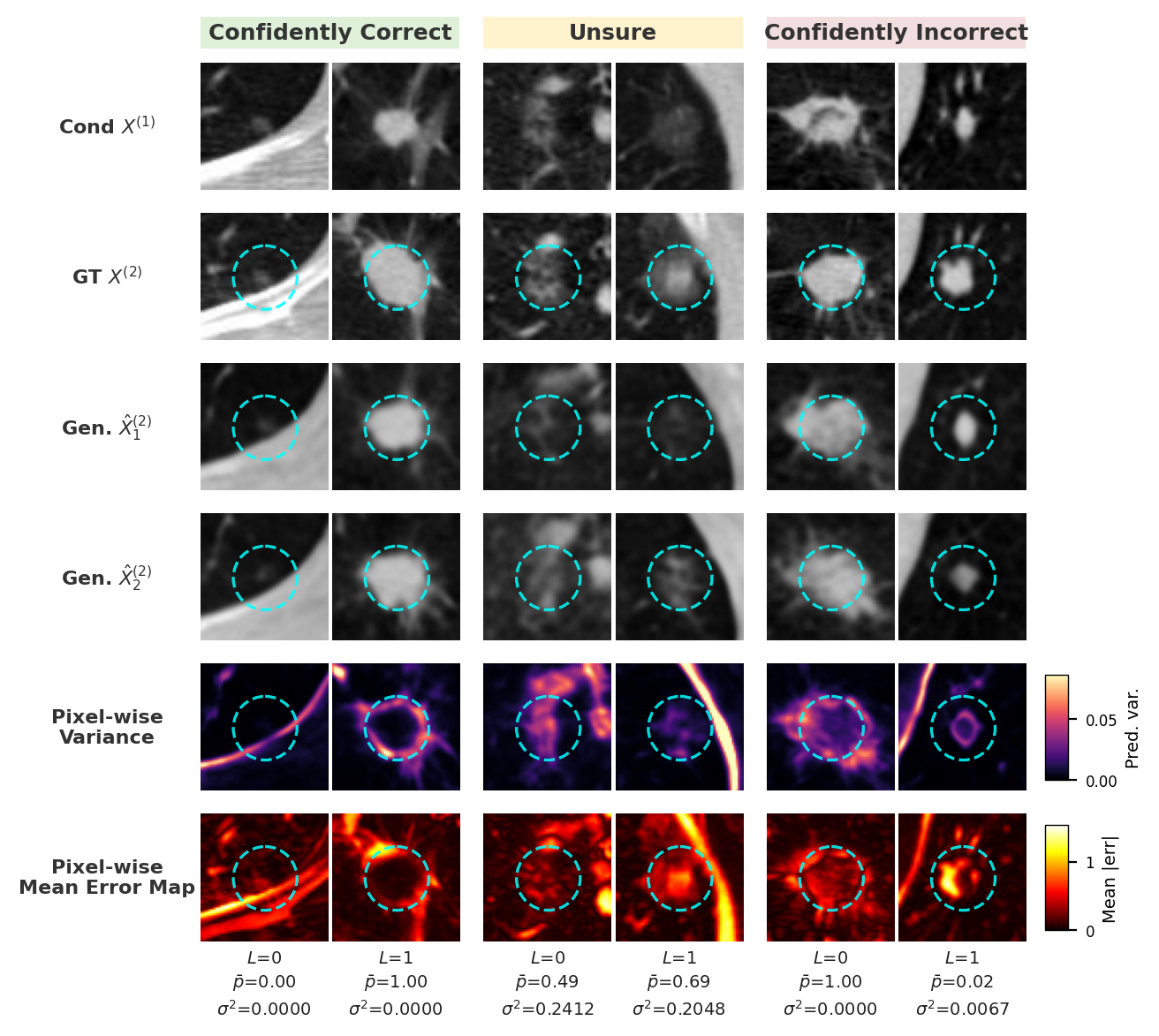
To better understand how the generated images influence diagnostic confidence, we analyzed the relationship between prediction error ($|L-\bar{p}|$, where $\bar{p}$ is the average probability across 20 runs), predictive variance ($\text{Var}(p)$), and the spatial characteristics of the generated images (Figure 3).

As shown in the left panels of Figure 3, the model’s output can be roughly split into three categories: predictions with low error and variance (confidently correct), predictions with median error and high variance (unsure), and predictions with high error and low variance (confidently incorrect). Both benign and malignant cases exist across these three cases. We also observe that both benign and malignant cases have predictions with low and high variance. Notably, benign cases have a lot of confident predictions compared to malignant cases.

We present qualitative assessments of the generated images across different confidence levels in the right panel of Figure 3. Notably, in the pixel-wise variance maps, the variance is predominantly concentrated along the boundary of the nodule rather than the interior. This suggests that the primary source of stochasticity in generated samples lies in subtle differences in nodule sizes and the background, rather than in the core morphological features. Moreover, the mean error maps show no clear distinction across confidence levels and correctness, showing that pixel-level fidelity to the ground truth images does not fully determine downstream diagnostic accuracy. This observation suggests that the generation task captures semantically meaningful representations that reflect the likely trajectory of nodule evolution. Accurately reconstructing the exact future appearance of a nodule is an inherently challenging task, due to the irreducible uncertainty in biological progression. However, we conjecture that pixel-wise reconstruction performance is not reflecting all the factors for downstream clinical prediction: NAMD achieves strong diagnostic performance despite slightly underperforming in image-quality metrics (Table 1). Instead, NAMD’s latent space encodes clinically relevant representations, such as the continuous progression change in nodule diameter as visualized in Figure 2. By encoding these clinically relevant progression signals rather than exact pixel-level detail, the generation task serves as an effective surrogate that captures disease trajectory signals, thereby improving early diagnostic accuracy.

5 Conclusion

We introduce Nodule-Aligned Multimodal Diffusion (NAMD), a framework for predicting longitudinal nodule progression that integrates a nodule-aligned latent space with an LLM-driven diffusion backbone. Our experiments show that NAMD generates follow-up images with diagnostic utility comparable to real follow-up LDCT scans, outperforming state-of-the-art baseline methods, competitive in terms of image quality, and allowing early disease diagnosis.

Appendix A Extended Related Work

Generative Models for Disease Progression Prediction

Generative models have emerged as a powerful tool for forecasting diseases. More recently, different strategies have relied on the use of diffusion models to achieve higher fidelity and stability. Initial applications focused on static image quality: for example, Weber et al. [2023] adopts cascaded latent diffusion models for high-resolution chest X-ray synthesis. Building on the generative capabilities, several approaches have been proposed for disease trajectory prediction. In the domain of chest X-rays, DDL-CXR [Yao et al., 2024] utilizes a Latent Diffusion Model to generate individualized Chest X-ray images for clinical prediction with asynchronous multi-modal clinical data; CXR-TFT [Arora et al., 2025] introduces a multi-modal transformer to predict chest X-rays over time. Extending beyond 2D data, Brain Latent Progression (BrLP) [Puglisi et al., 2025] proposes the use of ControlNet on latent diffusion models and an auxiliary model to synthesize individualized disease progression on 3D brain MRIs. More recently, some recent work has explored alternatives to standard diffusion methods: for example, ImageFlowNet [Liu et al., 2025a] optimizes deterministic or stochastic flow fields within a representation space across patients and timepoints using a ODE/SDE framework, and $\Delta-$LFM [Chen et al., 2026] proposes constructing a patient specific latent space by enforcing latents of MRIs from the same patient to lie on the same axis and using flow matching to model patient trajectories.

Conditional Generation with Diffusion Models

Diffusion models [Sohl-Dickstein et al., 2015, Ho et al., 2020] have become the dominant paradigm in generative models. Latent Diffusion Models (LDM) [Rombach et al., 2022] revolutionized high-resolution image synthesis by denoising in a compressed latent space, significantly reducing computational cost while maintaining perceptual quality. A key advantage of LDMs is their flexibility in incorporating conditional inputs such as text, images, or segmentation maps, to guide generation. ControlNet [Zhang et al., 2023] and T2I-Adaptor [Mou et al., 2023] introduced efficient adaptation modules for more precise spatial control without altering pretrained weights. Some recent advancements in DiTs [Peebles and Xie, 2023] have shown excellent controllability, with methods like OmniControl [Tan et al., 2025] demonstrating universal control capabilities within transformer-based backbones.

Despite these advancements, existing conditional methods largely target broad semantic alignment. They fail to take into account the subtle, continuous biological variations required for medical prognosis. Our work addresses this limitation by introducing a nodule-aligned latent space, which ensures that the generative process is governed by fine-grained clinical attributes rather than loose semantic or spatial guidance.

Appendix B Training Details

All NAMD training runs use the AdamW optimizer [Loshchilov and Hutter, 2019]. We adopt the VAE and U-Net architectures, along with pretrained weights, from Stable Diffusion v1.5 [Rombach et al., 2022]. The VAE has a latent dimension of 4 and a spatial compression factor of 8. The U-Net backbone follows the standard Stable Diffusion configuration, with 320 base channels, channel multipliers of [1, 2, 4, 4], two residual blocks per resolution, and eight attention heads.

We first fine-tune the VAE using Equation 6 with a learning rate of $5\times 10^{-5}$ and a batch size of 64. The U-Net is then fine-tuned for unconditional generation using a linear learning-rate warmup from $1\times 10^{-6}$ to $1\times 10^{-4}$ over 4,000 iterations, followed by cosine decay to a minimum learning rate of $1\times 10^{-5}$ over 100,000 steps, with a batch size of 16. Subsequently, the U-Net is further fine-tuned for conditional generation with a learning rate of $2\times 10^{-5}$ and a batch size of 8. We employ hybrid conditioning by concatenating condition image latents with the noisy latent, resulting in eight input channels, and by applying cross-attention with text embeddings extracted from MedGemma 1.5 4B (context dimension 2560). The diffusion process uses 1,000 timesteps with a linear noise schedule ranging from $\beta_{1}=8.5\times 10^{-4}$ to $\beta_{T}=1.2\times 10^{-2}$. Training is conducted for 60 epochs, with gradient clipping (maximum norm = 1.0), deterministic operations for reproducibility (seed = 23), and 32-bit floating-point precision.

Data augmentation includes random rotations of 45°, 90°, 135°, and 180°. The best-performing models are selected based on validation loss. For unconditional and conditional LDM training, we select later checkpoints right before overfitting. All experiments are performed on a single NVIDIA A40 GPU or L40 GPU.

Appendix C EHR Information and LLM Template

This section presents details on the 13 EHR features corresponding to each lung LDCT image as detailed in Table 2, as well as an example of a prompt that contains the feature information fed to the LLM later as detailed in Figure 4.

	Feature Name	Description	Value and Units
$\left.\vbox{\vrule height=0.0pt\multirow@dima width 0pt}\textnormal{{Nodule}}\right\{$	SCT_PRE_ATT	Predominant attenuation	Soft, Ground Glass, Part Solid
	SCT_EPI_LOC	Location of nodule in the lung	Right Upper/Middle/Lower lobe, Left Upper/Lower Lobe, Lingula
	SCT_LONG_DIA	Longest diameter	Millimeters
	SCT_PERP_DIA	Perpendicular diameter	Millimeters
	SCT_MARGINS	Margin of the nodule	Spiculated, Smooth, Poorly Defined
$\left.\vbox{\vrule height=0.0pt\multirow@dima width 0pt}\textnormal{{Patient}}\right\{$	age	Age	Years
	diagemph	Diagnosis to Emphysema	Yes/No
	gender	Gender	Male/Female
	famfather	Family history, Father	Yes/No
	fammother	Family history, Mother	Yes/No
	fambrother	Family history, Brother	Yes/No
	famsister	Family history, Sister	Yes/No
	famchild	Family history, Child	Yes/No
Legend: Continuous Variable $\cdot$ Multi-Category Variable $\cdot$ Binary Variable

Table 2: Description of the 13 features containing nodule and patient-level EHR information.

Figure 4: An example of a natural language prompt generated from the input features.

Appendix D Prediction Variance across runs

Figure 5: Running variance of ViT prediction probabilities across $K$ samples from the diffusion model for 50 datapoints. Each curve represents one datapoint.

Due to the stochastic nature of the diffusion sampling process via DDIM, the generated images will be slightly different with different initial noise. When these generated samples are evaluated by our downstream Vision Transformer (ViT), this diversity naturally translates into fluctuations in the predicted probabilities, which in turn causes variations in evaluation metrics such as AUROC and AUPRC. To determine an optimal $K$ value that balances evaluation stability with computational efficiency, we graph the running variance for 50 randomly sampled datapoints in Figure 5 and find the minimum $K$ where prediction variance stabilizes. As observed, the running variance for the majority of datapoints initially rises but plateaus after approximately $K=20$ samples. We therefore select $K=20$ for evaluation.