Discovery of interaction and diffusion kernels in particle-to-mean-field multi-agent systems

Abstract

We propose a data-driven framework to learn interaction kernels in stochastic multi-agent systems. Our approach aims at identifying the functional form of nonlocal interaction and diffusion terms directly from trajectory data, without any a priori knowledge of the underlying interaction structure. Starting from a discrete stochastic binary-interaction model, we formulate the inverse problem as a sequence of sparse regression tasks in structured finite-dimensional spaces spanned by compactly supported basis functions, such as piecewise linear polynomials. In particular, we assume that pairwise interactions between agents are not directly observed and that only limited trajectory data are available. To address these challenges, we propose two complementary identification strategies. The first based on random-batch sampling, which compensates for latent interactions while preserving the statistical structure of the full dynamics in expectation. The second based on a mean-field approximation, where the empirical particle density reconstructed from the data defines a continuous nonlocal regression problem. Numerical experiments demonstrate the effectiveness and robustness of the proposed framework, showing accurate reconstruction of both interaction and diffusion kernels even from partially observed. The method is validated on benchmark models, including bounded-confidence and attraction-repulsion dynamics, where the two proposed strategies achieve comparable levels of accuracy.

Keywords: multi-agent systems, data-driven methods, sparse-regression problems, mean-field dynamics, interaction kernel learning

MSC codes: 65L09, 70F17, 65C35, 35Q84

1 Introduction

The increasing availability of high-resolution data has stimulated a major research effort toward the discovery of differential equations directly from observations. In this setting, one typically assumes little or no a priori knowledge of the governing laws, and the objective is to reconstruct interpretable mathematical models from trajectory data. Among the various approaches in this direction we mention the Sparse Identification of Nonlinear Dynamics (SINDy) framework [9, 35, 36], which promotes sparse representations over candidate libraries for interpretable and efficient equation recovery, with extensions improving finite-data accuracy for stochastic [39] and partial differential equations [28]. Neural-network-based methodologies, such as Physics-Informed Neural Networks (PINNs) [24, 34], provide an alternative paradigm in which physical structure is embedded directly into learning architectures. In contrast, the present work formulates a regression problem to recover the governing mechanisms from data within structured finite-dimensional function spaces, yielding interpretable analytical approximations of the underling system. In particular, we focus on the discovery of interaction laws within multiscale agent systems similarly to recent approaches proposed in [7, 29], and motivated by data-driven models in socio-economic settings [2, 6].

Large systems of interacting agents constitute a fundamental modeling paradigm for describing hierarchical populations across a wide range of applications, including biological systems [5, 14], epidemiological dynamics [15, 16] and collective decision-making processes such as opinion formation [1, 17, 37]. In this setting, stochasticity and diffusion mechanisms are essential components of many interacting agent models, significantly affecting the emergence and large-scale organization of collective dynamics [18, 4]. Kinetic and mean-field descriptions of collective dynamics provide a multiscale modeling framework to connect microscopic interactions to macroscopic evolution laws [37, 17], where Boltzmann-type and Fokker–Planck equations are derived from binary interaction rules, see for example [10, 12, 32]. This hierarchy captures emergent collective behavior across particle, kinetic, and hydrodynamic levels. Extensions incorporating stochasticity, uncertainty, and heterogeneous interactions have been studied in several directions, e.g in [38, 33, 11].

Within this broad context, a rapidly growing research direction addresses the inverse problem of learning nonlocal interaction kernels from trajectory data, initiated in [7] and further developed into nonparametric learning frameworks with statistical guarantees in [27, 19, 26, 29] and numerical kernel-based reconstruction approaches [20]. These works establish consistency results and learning theory for the recovery of radial interaction kernels in deterministic and stochastic multi-agent systems, typically assuming access to multiple independent trajectories generated from different initial conditions. Related mean-field formulations with PDE-level stability estimates were proposed also in [13, 25]. Despite significant progress, most kernel-learning approaches assume full observability, focus primarily on drift identification, and rely on multiple trajectories for statistical stability. However, in practice interactions may be latent, dynamics inherently stochastic, and data limited, requiring for robust identification strategies with respect to partial observability and scarcity of data.

In this work, we address these challenges by developing a regression framework for the joint identification of nonlocal drift and diffusion interaction kernels in stochastic multi-agent systems with unobserved interaction structure. Inspired by particle-based simulation methods such as [30, 3, 23], we adopt a discrete stochastic binary-interaction model to describe the underlying agent dynamics. This modeling choice provides a natural bridge between microscopic interactions and macroscopic collective behavior, ensuring multiscale consistency [8, 22]. Hence, the inverse problem is formulated as a regression task in finite-dimensional linear spaces spanned by compactly supported piecewise linear basis functions, where two main challenges arise due to limited availability of independent trajectories and the unobservability of pairwise interactions. To cope with these issues, we propose two different strategies. First, we use a random-batch regression approach to manage latent interactions via randomly sampled subsets, reducing computational complexity while preserving the statistical structure in expectation. Furthermore, we establish a connection with a mean-field formulation in which the empirical density is reconstructed from the data, and defining a continuous nonlocal regression problem. This macroscopic perspective is subsequently integrated into the reconstruction process, enhancing the robustness and stability of the overall identification framework. We also provide a priori error estimates that account for the fact that the reconstructed trajectories do not use information on the interaction between particles. Numerical experiments confirm that this approach accurately reconstructs finite-dimensional approximations of both drift and diffusion interaction kernels in noisy and data-limited regimes, demonstrating its effectiveness and scalability for inverse problems in stochastic interacting particle systems.

The manuscript is organized as follows. In Section 2, we introduce the modeling hierarchy and the binary interaction dynamics underlying the learning problem. Section 3 presents the identification of interaction and diffusion kernels under full observability of the pairwise interactions. Sections 3.2 and 3.3 address the case of partial observability via random-batch and mean-field approaches, respectively. Section 4 provides an a priori error estimate for the reconstructed trajectories. Section 5 presents numerical experiments assessing the performance of the proposed methods, and final conclusions are drawn in Section 6.

2 Model hierarchy for pairwise interacting agent systems

We consider a system of $N$ agents characterized at discrete time $t_{n}$ by features $\{x_{i}^{n}\}_{i=1}^{N}$, with $x_{i}^{n}\in\mathbb{R}^{d}$. Interactions occur pairwise, over a time step $[t_{n},t_{n}+\Delta t]$ each agent $i\in\{1,\dots,N\}$ interacts with a selected agent $j(i)$, and the post-interaction states are updated according to

$$x_{i}^{n+1} =x_{i}^{n}+\Delta t\,P(x_{i}^{n},x_{j(i)}^{n})(x_{j(i)}^{n}-x_{i}^{n})+\sqrt{\Delta t}\,D(x_{i}^{n},x_{j(i)}^{n})\,\xi_{ij(i)}^{n},$$ (1)

$$x_{j(i)}^{n+1} =x_{j(i)}^{n}+\Delta t\,P(x_{j(i)}^{n},x_{i}^{n})(x_{i}^{n}-x_{j(i)}^{n})+\sqrt{\Delta t}\,D(x_{j(i)}^{n},x_{i}^{n})\,\xi_{j(i)i}^{n},$$

where $P,D:\mathbb{R}^{d}\times\mathbb{R}^{d}\to\mathbb{R}$ weight the compromise and stochastic fluctuation mechanisms. The random vectors $\xi_{ij}^{n}$ are i.i.d. with zero mean and covariance $\mathbb{E}[\xi_{ij}^{n}(\xi_{ij}^{n})^{\top}]=\mathsf{I}_{d}$.

The microscopic rule (1) defines a discrete-time stochastic process on $\mathbb{R}^{dN}$. Randomness enters in the microscopic dynamics through two mechanisms: the stochastic fluctuations $\xi_{ij}^{n}$ acting at each binary interaction, and the random selection of partners $j(i)$ at every time step. As a result, the system evolves through stochastic pairwise interactions rather than deterministic averaged forces. Such binary random interactions constitute the elementary mechanism underlying random-batch approximations of mean-field particle systems and, in the large population limit, admit an equivalent kinetic representation in terms of the one particle distribution function. The following subsections detail these connections.

2.1 Mean-field dynamics via random-batch approximation

The binary scheme (1) can be interpreted as the building block of a stochastic random-batch approximation of a fully interacting system. At time step $n$, each agent $i$ interacts with a random subset $J_{i}^{n}\subset\{1,\dots,N\}\setminus\{i\}$ of size $N_{p}\ll N$, leading to

$$x_{i}^{n+1}=x_{i}^{n}+\frac{\Delta t}{N_{p}}\sum_{j\in J_{i}^{n}}P(x_{i}^{n},x_{j}^{n})(x_{j}^{n}-x_{i}^{n})+\frac{\sqrt{\Delta t}}{N_{p}}\sum_{j\in J_{i}^{n}}D(x_{i}^{n},x_{j}^{n})\,\xi_{ij}^{n}.$$ (2)

Under the assumption that, for each fixed $i$ and $n$, the set $J_{i}^{n}$ is sampled uniformly among all subsets of $\{1,\dots,N\}\setminus\{i\}$ of cardinality $N_{p}$, independently of the particle configuration and of previous time steps, the random-batch approximation provides an unbiased estimator of the full interaction operators. Hence, passing formally to the limit $\Delta t\to 0$ and setting $N_{p}=N$ yield the continuous-time interacting particle system

$$dx_{i}=\frac{1}{N}\sum_{j=1}^{N}P(x_{i},x_{j})(x_{j}-x_{i})\,dt+\frac{1}{N}\sum_{j=1}^{N}D(x_{i},x_{j})\,dB_{ij},$$ (3)

where $(B_{ij})_{i,j}$ are independent Brownian motions. This stochastic differential system represents the mean-field interaction of agents driven by averaged compromise and cumulative stochastic perturbations.

In the limit $N\to\infty$, we assume that the interaction kernels $P$ and $D$ are globally Lipschitz continuous and of at most linear growth, ensuring well-posedness of the interacting particle system. We further assume that the initial data are independent identically distributed with law $f_{0}\in\mathcal{P}_{2}(\mathbb{R}^{d})$ and that the driving Brownian motions are independent. Under these assumptions, classical propagation of chaos results yield convergence of the empirical measure toward a nonlinear McKean-Vlasov process, whose law $f(x,t)$ solves the nonlocal Fokker-Planck equation

$$\partial_{t}f(x,t)=-\,\nabla_{x}\!\cdot\!\left(f(x,t)\,\mathcal{P}[f](x,t)-\frac{1}{2}\,\nabla_{x}\!\bigl(f(x,t)\,\mathcal{D}[f](x,t)\bigr)\right),$$ (4)

where

$$\mathcal{P}[f](x,t) =\int_{\mathbb{R}^{d}}P(x,x_{*})(x_{*}-x)\,f(x_{*},t)\,dx_{*},$$

$$\mathcal{D}[f](x,t) =\int_{\mathbb{R}^{d}}D(x,x_{*})^{2}\,f(x_{*},t)\,dx_{*},$$

see for example [21] for a general reference.

2.2 Kinetic description via binary interactions

In the mean-field regime $N\to\infty$, under exchangeability and propagation of chaos, the interacting particle system admits a mesoscopic description in terms of the one particle density $f(x,t)$. Within the kinetic framework, interactions are modeled as stochastic binary collisions between statistically independent agents with joint distribution $f(x,t)f(x_{*},t)$.

In this context, the binary interaction mechanism associated with (1) can be written in the equivalent form as

$$x^{\prime} =x+\delta\,P(x,x_{*})(x_{*}-x)+\sqrt{\delta}\,D(x,x_{*})\,\xi,$$ (5)

$$x_{*}^{\prime} =x_{*}+\delta\,P(x_{*},x)(x-x_{*})+\sqrt{\delta}\,D(x_{*},x)\,\xi_{*},$$

where $(x,x_{*})$ and $(x^{\prime},x_{*}^{\prime})$ denote the pre- and post-interaction states, respectively, $\delta>0$ measures the interaction strength, and $\xi,\xi_{*}$ are centered random vectors describing stochastic fluctuations. The evolution of the particle density $f(\cdot)$ can be described by a Boltzmann-type equation of the following form

$$\partial_{t}f(x,t)=Q(f,f)(x,t),$$ (6)

with interaction operator

$$Q(f,f)(x)=\mathbb{E}\!\left[\lambda\int_{\mathbb{R}^{d}}\left(\frac{1}{J^{\prime}}f(x^{\prime})f(x_{*}^{\prime})-f(x)f(x_{*})\right)dx_{*}\right],$$ (7)

where $J^{\prime}$ is the Jacobian of the transformation $(x,x_{*})\mapsto(x^{\prime},x_{*}^{\prime})$ and $\lambda>0$ is the interaction frequency, see for example [37, 32].

Quasi-invariant interaction limit and Fokker–Planck equation

In weak form, for any test function $\varphi\in C_{c}^{2,\alpha}(\mathbb{R}^{d})$, with $\alpha\in(0,1]$, we can write

$$\frac{d}{dt}\int_{\mathbb{R}^{d}}\varphi(x)f(x,t)\,dx={\lambda}\iint_{\mathbb{R}^{2d}}\mathbb{E}\!\left[\varphi(x^{\prime})-\varphi(x)\right]f(x,t)f(x_{*},t)\,dx\,dx_{*}.$$ (8)

To derive the macroscopic limit, we consider the quasi-invariant scaling

$$\delta=\varepsilon,\qquad\mathbb{E}[\xi^{2}]=\varepsilon,\qquad\lambda={1}/{\varepsilon},\qquad 0<\varepsilon\ll 1,$$ (9)

corresponding to high frequency but weak interactions. Then the scaled dynamics reads

$$x^{\prime}-x=\varepsilon P(x,x_{*})(x_{*}-x)+\sqrt{\varepsilon}D(x,x_{*})\xi,$$

and using Taylor’s expansion up to second order for $\varphi\in C_{c}^{2,\alpha}(\mathbb{R}^{d})$ we have

$$\varphi(x^{\prime})-\varphi(x)=\nabla\varphi(x)\cdot(x^{\prime}-x)+\frac{1}{2}(x^{\prime}-x)^{\top}\nabla^{2}\varphi(x)(x^{\prime}-x)+\mathcal{O}(|x^{\prime}-x|^{2+\alpha}).$$

Then, the limiting Fokker-Planck equation (4) is recovered in weak form for every test function $\varphi\in C_{c}^{2,\alpha}(\mathbb{R}^{d})$ for $0<\alpha\leq 1$. Indeed, using the previous Taylor expansion in (8) and controlling the reminder, in the limit for $\varepsilon\to 0$ one obtains the following equation

$$\frac{d}{dt}\int_{\mathbb{R}^{d}}\varphi(x)\,f(x,t)\,dx=$$ (10)

$$\qquad\int_{\mathbb{R}^{d}}\nabla\varphi(x)\cdot\mathcal{P}[f](x,t)\,f(x,t)\,dx+\frac{1}{2}\int_{\mathbb{R}^{d}}\Delta\varphi(x)\,\mathcal{D}[f](x,t)\,f(x,t)\,dx.$$

Integration by parts gives the strong nonlinear Fokker-Planck, which coincides with the forward Kolmogorov equation (4) associated with the nonlinear mean-field stochastic dynamics (3), providing consistency between the microscopic, kinetic, and mean-field descriptions of the model hierarchy. We refer for further details on this limit to [37, 32].

3 Discovery of drift and diffusion interaction kernels

The discrete dynamics (1) of the ensemble of $N$ agents can be conveniently written in a vectorized form, introducing the full vector $X^{n}\in\mathbb{R}^{dN}$ that collects the agent states in $d$-blocks, i.e., $X^{n}=\mathrm{vec}(x_{1}^{n},\ldots,x_{N}^{n})\in\mathbb{R}^{dN}$, where $x_{i}^{n}\in\mathbb{R}^{d}$ is the feature of $i$-agent at time $t_{n}:=n\Delta t$ with $n=0,\ldots,M$. To identify the interacting agent associated to each $i$-agent, we consider the permutation matrix $S^{n}\in\mathbb{R}^{N\times N}$ encoding pairings at time step $n$, and define the block action on $\mathbb{R}^{dN}$ by

$$\mathsf{S}^{n}:=S^{n}\otimes\mathsf{I}_{d}\in\mathbb{R}^{dN\times dN},$$

where the interacting $j(i)$-agent is given by $(\mathsf{S}^{n}X^{n})_{i}=x_{j(i)}^{n}$. Then, the vectorized form of the full dynamics (1) reads as

$$X^{n+1}=X^{n}+\Delta t\,\mathbf{P}^{n}\odot\big(\mathsf{S}^{n}X^{n}-X^{n}\big)+\sqrt{\Delta t}\,\mathbf{D}^{n}\odot\Xi^{n},$$ (11)

where $\odot$ stands for the Hadamard product. In (11) we introduce, through the Kronecker product $\otimes,$ the vectorized interaction and diffusion coefficients

$$\mathbf{P}^{n}:=P^{n}\otimes\mathbf{1}_{d}\in\mathbb{R}^{dN},\qquad\mathbf{D}^{n}:=D^{n}\otimes\mathbf{1}_{d}\in\mathbb{R}^{dN},$$

where $P^{n},D^{n}\in\mathbb{R}^{N}$ collect the scalar weights associated with each agent at time $t_{n}$, and $\mathbf{1}_{d}=(1,\ldots,1)^{\top}\in\mathbb{R}^{d}$ replicates them over the $d$ components of each block. Specifically, the entries of $P^{n}$ and $D^{n}$ are given by

$$P_{i}^{n}=P(x_{i}^{n},x_{j(i)}^{n}),\qquad D_{i}^{n}=D(x_{i}^{n},x_{j(i)}^{n}),$$ (12)

corresponding to the values of the interaction and diffusion functions evaluated on the current pair $(x_{i}^{n},x_{j(i)}^{n})$. Finally, we consider $\Xi^{n}\in\mathbb{R}^{dN}$ to be the stacked noise as a collection of each of the random variables $\xi_{i}^{n}\in\mathbb{R}^{d}$, i.e. $\Xi^{n}=(\xi^{n}_{1},\ldots,\xi_{N}^{n})^{\top}$. The stochastic discrete dynamics (11) describes the microscopic evolution of interacting agents driven by deterministic pairwise interactions and random perturbations. Due to the random pairing matrices $S^{n}$ and stochastic terms $\Xi^{n}$, the trajectories are random processes even when $P$ and $D$ are deterministic.

Our main goal is to reconstruct suitable approximations of the interaction kernel $P(\cdot)$ and diffusion function $D(\cdot)$ from observed data, following approaches similar to [7, 19, 26]. Hence, given the agent trajectories samples $\{X^{n}\}_{n=0}^{M}$, we seek interaction and diffusion operators that best explain the observed dynamics, namely

$$(P^{*},D^{*})=\operatorname*{argmin}_{P\in\mathscr{A}_{P},\;D\in\mathscr{A}_{D}}\mathcal{E}\big(P,D;\{X^{n}\}_{n=0}^{M}\big),$$ (13)

where $\mathscr{A}_{P}$ and $\mathscr{A}_{D}$ are admissible classes of interaction and diffusion functions defined below, and $\mathcal{E}$ is a suitable empirical loss functional encoding the discrepancy between the model dynamics (1) and the observed trajectories.

In the remainder of this manuscript we will focus on the relevant case of radial interaction kernels and diffusions in (12), namely we assume

$$P(x,y)=P(r),\qquad D(x,y)=D(r),\qquad r:=\lvert|x-y\rvert|,$$

which is standard framework in interacting particle systems such as opinion dynamics, aggregation models, or flocking systems. Nevertheless, the main difficulties of the reconstruction problem remain unchanged, since the stochasticity of the dynamics and the lack of observability of the interaction pairs still lead to ill-posed inverse formulations.

To realize the inverse problem (13) we introduce a finite-dimensional approximation in terms of a family of one-dimensional non-negative basis functions $\{\Phi_{k}(\cdot)\}_{k\geq 1}$ and $\{\Psi_{k}(\cdot)\}_{k\geq 1}$. Specifically, we selected a family of piecewise linear and compactly supported basis functions defined on suitable discretizations of the domains of $P$ and $D$ (see an example in Figure 1).

Figure 1: Case of domain $[0,2]$, example of $N_{b}^{P}=5$ piecewise linear basis functions on a uniform mesh (left) and on a Chebyshev mesh (right).

Thus, we can introduce the approximation spaces that we will use in (13) as follows

$$\mathscr{A}_{P}:=\mathrm{span}\{\Phi_{1},\ldots,\Phi_{N_{b}^{P}}\},\qquad\mathscr{A}_{D}:=\mathrm{span}\{\Psi_{1},\ldots,\Psi_{N_{b}^{D}}\},$$

with respective dimensions $N_{b}^{P}$ and $N_{b}^{D}$ and the approximations of the drift and diffusion kernels read as

$$\widehat{P}(r):=\sum_{k=1}^{N_{b}^{P}}\varrho_{k}\,\phi_{k}(r),\qquad\widehat{D}^{2}(r):=2\sum_{k=1}^{N_{b}^{D}}\zeta_{k}\,\psi_{k}(r),$$ (14)

where $\varrho\in\mathbb{R}^{N_{b}^{P}}$ and $\zeta\in\mathbb{R}^{N_{b}^{D}}$ are the vector coefficient to be determined by means of the optimization problem (13).

We introduce the design matrices ${\bf\Theta}^{n}=[\Theta_{1}^{n},\ldots,\Theta_{N_{b}^{P}}^{n}]\in\mathbb{R}^{dN\times N_{b}^{P}}$ and ${\bf\Lambda}^{n}=[\Lambda_{1}^{n},\ldots,\Lambda_{N_{b}^{D}}^{n}]\in\mathbb{R}^{dN\times N_{b}^{D}}$ such that their $k-$th columns at time $t_{n}$ are given by

$$\Theta^{n}_{k} =\phi_{k}\!\left(\,\lVert{S}^{n}X^{n}-X^{n}\rVert\,\right)\odot\bigl({S}^{n}X^{n}-X^{n}\bigr),\qquad k=1,\ldots,N_{b}^{P},$$ (15)

$$\Lambda^{n}_{k} =\psi_{k}\!\left(\,\lVert{S}^{n}X^{n}-X^{n}\rVert\,\right),\qquad k=1,\ldots,N_{b}^{D},$$

then the microscopic dynamics (11) can be rewritten as follows

$$X^{n+1}=X^{n}+\Delta t{\bf\Theta}^{n}\varrho+\sqrt{2\Delta t{\bf\Lambda}^{n}\zeta}\odot\Xi^{n}.$$ (16)

Hence, the identification problems (13) can be addressed considering two different least square problems, one for the drift as

$$\varrho^{*}=\operatorname*{argmin}_{\varrho\in\mathcal{A}_{P}}\frac{1}{M_{P}}\sum_{n=1}^{M_{P}}\left\|X^{n+1}-X^{n}-\Delta t\,\mathbb{E}\left[{\bf\Theta}^{n}\varrho|X^{n}\right]\right\|^{2},$$ (17)

and one for the diffusion as

$$\zeta^{*}=\operatorname*{argmin}_{\zeta\in\mathcal{A}_{D}}\frac{1}{M_{D}}\sum_{n=1}^{M_{D}}\left\|\bigl(X^{n+1}-X^{n}\bigr)\odot\bigl(X^{n+1}-X^{n}\bigr)-2\Delta t\,\mathbb{E}\left[{\bf\Lambda}^{n}\zeta|X^{n}\right]\right\|^{2},$$ (18)

where the conditional expectation $\mathbb{E}[\cdot|X^{n}]$ is taken with respect to the stochastic variables associated with the noise term $\Xi^{n}$ and the random pairing matrix $\mathsf{S}^{n}$. Note that potentially different numbers of snapshots $M_{P},M_{D}\leq M$ can be employed for each problem. The admissibility constraints $\mathscr{A}_{P}$ and $\mathscr{A}_{D}$ are now enforced through the coefficient spaces. For the drift, we use the constrained space

$$\mathcal{A}_{P}=\left\{\rho\in\mathbb{R}^{N_{b}^{P}}:\rho_{1}=\overline{\rho},\,\kappa_{P}\rho_{k}\leq\kappa_{P}\rho_{k+1},\,k=1,\dots,N_{b}^{P}\right\},$$ (19)

with $\overline{\rho}$ value of the kernel in $r=0$, $\kappa_{P}=1$ for repulsive dynamics, $\kappa_{P}=-1$ for attractive ones, while for $\kappa_{P}=0$ we do not impose any monotonicity. For the diffusion, instead, we impose non-negativity via

$$\mathcal{A}_{D}:=\left\{\zeta\in\mathbb{R}^{N_{b}^{D}}:\ \zeta_{k}\geq 0,\,\kappa_{D}\zeta_{k}\leq\kappa_{D}\zeta_{k+1},\ k=1,\ldots,N_{b}^{D},\,\zeta_{i}=\overline{\zeta}_{i}\mbox{ for some }i\right\}.$$ (20)

where the coefficients $\kappa_{D}$ play the same role of $\kappa_{P}$ in (19). This choice of $\mathcal{A}_{D}$ ensures that the reconstructed diffusion coefficient $\widehat{D}(r)^{2}$ in (14) remains non-negative on the reconstruction grid.

Remark 1.

In general, the interaction matrices $\mathsf{S}^{n}$ governing the microscopic dynamics are not directly observable from trajectory data, and they constitutes a source of uncertainty in the reconstruction problem, affecting both the statistical variability of the data and the effective exploration of the dynamics. As a consequence, the stochastic evolution (11) cannot be identified pathwise and must instead be reconstructed in a statistical sense. To this end, in the previous general formulation, we rely on Itô–Taylor expansions to derive suitable moment-based approximations of the drift and diffusion terms from the observed trajectories, which form the basis of the least squares problem (13). More precisely, for the interaction rule (11), the following relations hold at each time step for the drift term

$$\mathbb{E}\!\left[\mathbf{P}^{n}\odot\bigl(\mathsf{S}^{n}X^{n}-X^{n}\bigr)\;\middle|\;X^{n}\right]=\frac{1}{\Delta t}\,\mathbb{E}\!\left[X^{n+1}-X^{n}\;\middle|\;X^{n}\right]+\mathcal{O}(\Delta t),$$ (21)

and for the diffusion term

$$\frac{1}{2}\,\mathbb{E}\!\left[\bigl(\mathbf{D}^{n}\odot\mathbf{D}^{n}\bigr)\;\middle|\;X^{n}\right]=\frac{1}{2\,\Delta t}\mathbb{E}\!\left[\bigl(X^{n+1}-X^{n}\bigr)\odot\bigl(X^{n+1}-X^{n}\bigr)\;\middle|\;X^{n}\right]+\mathcal{O}(\Delta t),$$ (22)

where the conditional expectations are taken with respect to both the latent interaction variables $\mathsf{S}^{n}$ and the microscopic noise realizations $\Xi^{n}$, conditioned on the observed state $X^{n}$. These expansions show that, at leading order in $\Delta t$, the drift and diffusion contributions can be approximated independently through the first and second conditional moments of the observed increments. In the following, we first analyze an idealized setting in which the interaction matrices $\mathsf{S}^{n}$ are assumed to be known. This assumption will be relaxed in a subsequent section, where the effects of latent interactions are explicitly taken into account.

3.1 Kernel estimations with known interaction matrices

We first assume to have the dataset $\left\{t_{n},X^{n},\mathsf{S}^{n}\right\}_{n=0}^{M}$, meaning that we have access to the state of the agents at certain times $t_{n}$ and also to their pairwise interaction matrix $\mathsf{S}^{n}$. Given this information over $M_{P}\leq M$ time frames, the coefficients of the interaction kernel are obtained by solving the least-squares problem

$$\varrho^{*}=\operatorname*{argmin}_{\varrho\in\mathbb{R}^{N_{b}^{P}}}\frac{1}{M_{P}}\sum_{n=1}^{M_{P}}\left\|X^{n+1}-X^{n}-\Delta t\,{\bf\Theta}^{n}\varrho\right\|^{2}.$$ (23)

Here, in contrast to (17), the interaction matrices $\mathsf{S}^{n}$ are assumed to be known. As a consequence, all interaction dependent quantities, such as the increments $\mathsf{S}^{n}X^{n}-X^{n}$ and their associated basis function evaluations, are directly observable from the data. The resulting estimator is therefore affected solely by the statistical fluctuations induced by the stochastic noise, and not by uncertainty in the underlying pairing patterns. This reduced source of variability generally leads to better conditioned least squares problems and more stable parameter estimates. Similarly, for the diffusion interaction kernel we consider in general $M_{D}\leq M$ time frames. The diffusion coefficients are determined from

$$\zeta^{*}=\operatorname*{argmin}_{\zeta\in\mathcal{A}_{D}}\frac{1}{M_{D}}\sum_{n=1}^{M_{D}}\left\|\bigl(X^{n+1}-X^{n}\bigr)\odot\bigl(X^{n+1}-X^{n}\bigr)-2\Delta t\,{\bf\Lambda}^{n}\zeta\right\|^{2},$$ (24)

where ${\bf\Lambda}^{n}$ is defined columnwise as in (15).

Both (23) and (24) can be cast as quadratic programs with linear constraints and solved with standard constrained least-squares solvers. Here we adopt an interior-point method [31], other suitable choices include projected-gradient methods, active-set algorithms, or nonnegative least-squares (NNLS). Moreover, since the estimators (23) and (24) are fully decoupled, they can be computed independently and may use different time windows and sample sizes, so in general we allow $M_{P}\neq M_{D}$.

Test 1: numerical validation for known interaction matrices

We consider a system of $N=10^{5}$ interacting agents and $M=201$ snapshots of the dynamics, uniformly sampled with time step $\Delta t=0.01$. The interaction kernel governing the drift is given by

$$P(r)=(1+r^{2})^{-2},$$

while the diffusion term is defined through the pairwise interaction

$$D(x,y)=\tilde{D}(\lvert x-y\rvert)\,(y-x),\qquad\tilde{D}(r)={0.25}/{(1+r)^{2}}.$$

Thus, we are interested in reconstructing the kernel $P$ and the radial part of the diffusion, meaning $\tilde{D}$. Notice that the functional form of $D(x,y)$ is slightly more general than the one considered in the theoretical discussion above. However, this additional structure does not affect the proposed reconstruction procedure.

We choose $N_{b}^{P}=10$ basis functions for the kernel reconstruction and $N_{b}^{D}=8$ basis functions for the diffusion, and we use $M_{P}=20$, and $M_{D}=10$ consecutive time frames for the learning process, meaning that we only look up to time $t=0.2$ for the kernel reconstruction and up to time $t=0.1$ for the diffusion, even with an available time horizon of $[0,2]$.

Figure 2: Test 1: Reconstructed kernel $P(r)=(1+r^{2})^{-2}$ (left) using $N^{P}_{b}=10$ basis functions, reconstructed radial density $D(r)=0.25/(1+r)^{2}$ using $N^{D}_{p}=8$ basis functions (center), comparison between the data density $f$ and the reconstructed $\widehat{f}$ at the final time (right).

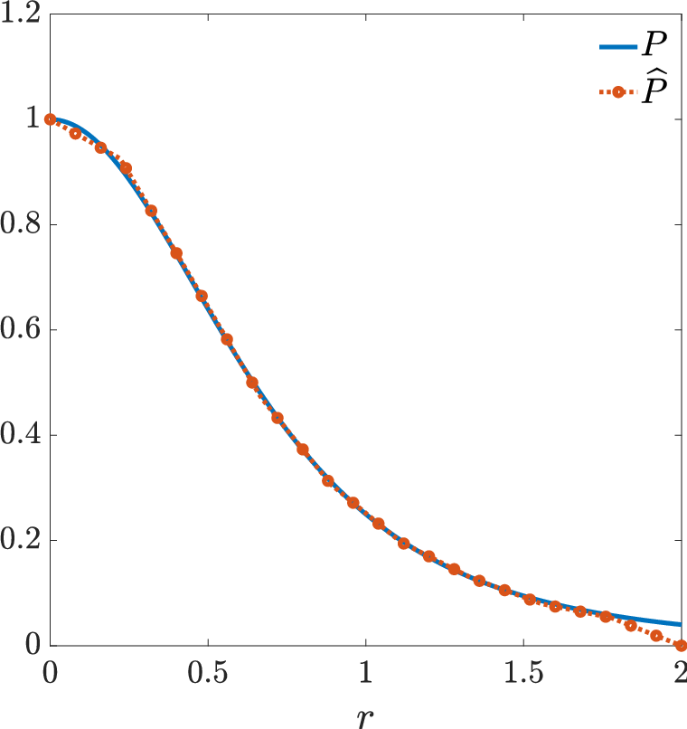
Figure 2 shows (left) the exact interaction kernel $P$ together with its reconstruction $\widehat{P}$, (center) the exact radial diffusion profile $\tilde{D}$ and its reconstruction $\widehat{\tilde{D}}$, and (right) the particle density at various times. The latter is compared with the reconstructed density $\widehat{f}(\cdot,t)$ obtained by simulating the particle dynamics (11) with the learned kernels $\widehat{P}$ and $\widehat{D}$, getting the reconstructed particle trajectories $\widehat{X}^{n}=\textrm{vec}(\widehat{x}_{1}^{n},\dots,\widehat{x}_{N}^{n})$. The empirical densities associated with the exact and reconstructed particle systems are defined as

$$f(x,t_{n}):=\frac{1}{N}\sum_{i=1}^{N}\delta\!\bigl(x-X_{i}^{n}\bigr),\qquad\widehat{f}(x,t_{n}):=\frac{1}{N}\sum_{i=1}^{N}\delta\!\bigl(x-\widehat{X}_{i}^{n}\bigr).$$

To quantify the reconstruction accuracy, for a generic target function $F$ and its approximation $\widehat{F}$ we consider the relative errors

$$E_{F}^{1}:=\frac{\|{F}-\widehat{F}\|_{L^{1}(I)}}{\|{F}\|_{L^{1}(I)}},\qquad E_{F}^{\infty}:=\frac{\|{F}-\widehat{F}\|_{L^{\infty}(I)}}{\|{F}\|_{L^{\infty}(I)}},$$ (25)

with $I=[0,2]$ for $F\equiv P$ and for $F\equiv\tilde{D}$.

To quantify the accuracy of the reconstructed trajectories, we define the time-averaged and final-time reconstruction errors

$$E_{f}^{\mathrm{ave}}:=\frac{1}{N_{T}}\sum_{n=1}^{N_{T}}W_{1}(X^{n},\widehat{X}^{n}),\qquad E_{f}^{\mathrm{fin}}:=W_{1}(X^{N_{T}},\widehat{X}^{N_{T}}),$$ (26)

which measure the discrepancy between the empirical densities $f(\cdot,t_{n})$ and $\widehat{f}(\cdot,t_{n})$, and where we use the $1$-Wasserstein distance between the empirical measures associated with the particle configurations $X^{n}$ and $\widehat{X}^{n}$ at time $t_{n}$, denoted by $W_{1}(X^{n},\widehat{X}^{n})$. In one spatial dimension, this distance admits the explicit representation

$$W_{1}(X^{n},\widehat{X}^{n})=\frac{1}{N}\sum_{i=1}^{N}\bigl|x_{\pi(i)}^{n}-\widehat{x}_{\pi^{\prime}(i)}^{n}\bigr|,$$

where $x_{\pi(i)}^{n}$ and $\widehat{x}_{\pi^{\prime}(i)}^{n}$ denote the sorted samples of the two particle ensembles.

In this simulation, the kernel reconstruction errors are $E_{P}^{1}=1.49\cdot 10^{-2}$ and $E_{P}^{\infty}=4.00\cdot 10^{-2}$, while the diffusion errors are $E_{D}^{1}=3.68\cdot 10^{-2}$ and $E_{D}^{\infty}=6.65\cdot 10^{-2}$. Moreover, the density reconstruction errors are $E_{f}^{\mathrm{ave}}=1.09\cdot 10^{-3}$ and $E_{f}^{\mathrm{fin}}=1.31\cdot 10^{-3}$. We summarize the error in table 1.

	$F\equiv P$	$F\equiv D$
$E_{F}^{1}$	$1.49\cdot 10^{-2}$	$3.68\cdot 10^{-2}$
$E_{F}^{\infty}$	$4.00\cdot 10^{-2}$	$6.65\cdot 10^{-2}$

$E_{f}^{\mathrm{ave}}$	$1.09\cdot 10^{-3}$
$E_{f}^{\mathrm{fin}}$	$1.31\cdot 10^{-3}$

Table 1: Test 1: Relative reconstruction errors for the interaction kernel $P$ and diffusion $D$ and for the empirical density $f(\cdot)$.

3.2 Random-batch kernel estimation with unknown interaction pairs

In the general setting, the available data consist only of agent trajectories $\{t_{n},X^{n}\}_{n=0}^{M}$, while the pairing matrices $\mathsf{S}^{n}$ and noise realizations $\Xi^{n}$ remain unobserved.

In this setting, to approximate the conditional expectations in (17) and (18) we replace it with a collection of randomly generated batch interaction maps $S^{(h,n)},\ h=1,\ldots,N_{p}$, where each $S^{(h,n)}$ is a permutation matrix selecting one random interacting pair and $N_{p}\ll N$ denotes the number of sampled pairs. The conditional expectations are then approximated by empirical averages over these sampled batches, and given this information over $M_{P}\leq M$ time frames for the drift kernel, the coefficients are obtained by solving

$$\varrho^{*}=\operatorname*{argmin}_{\varrho\in\mathbb{R}^{N_{b}^{P}}}\frac{1}{M_{P}}\sum_{n=1}^{M_{P}}\left\|X^{n+1}-X^{n}-\frac{\Delta t}{N_{p}}\sum_{h=1}^{N_{p}}{\bf\Theta}^{(n,h)}\,\varrho\right\|^{2},$$ (27)

where

$${\bf\Theta}^{(n,h)}:={\bf\Theta}\left(\|{S}^{(n,h)}X^{n}-X^{n}\|\right)\odot\left({S}^{(n,h)}X^{n}-X^{n}\right)\in\mathbb{R}^{dN\times N_{b}^{P}}.$$

Here, differently from (23), the interaction matrices are unknown and must be approximated through random batching. This introduces additional variability beyond the statistical fluctuations from stochastic noise, as the estimator now depends on both the noise realization and the uncertainty in pairing patterns.

Similarly, for the diffusion interaction kernel we consider in general $M_{D}\leq M$ time frames. The diffusion coefficients are determined from

$$\zeta^{*}=\operatorname*{argmin}_{\zeta\in\mathcal{A}_{D}}\frac{1}{M_{D}}\sum_{n=1}^{M_{D}}\left\|\bigl(X^{n+1}-X^{n}\bigr)\odot\bigl(X^{n+1}-X^{n}\bigr)-\frac{2\Delta t}{N_{p}}\sum_{h=1}^{N_{p}}{\bf\Lambda}^{(n,h)}\zeta\right\|^{2},$$ (28)

where

$${\bf\Lambda}^{(n,h)}:={\bf\Lambda}\left(\|{S}^{(n,h)}X^{n}-X^{n}\|\right)\in\mathbb{R}^{dN\times N_{b}^{D}}.$$

These formulations provide unbiased Monte Carlo approximations of the drift and diffusion contributions, enabling kernel reconstruction through batch averaging in analogy with the random batch method (2). In particular, the scheme

$$X^{n+1}=X^{n}+\frac{\,\Delta t}{N_{p}}\sum_{h=1}^{N_{p}}{\bf\Theta}^{(n,h)}\,\varrho+\left(\sqrt{\frac{2\,\Delta t}{N_{p}}\sum_{h=1}^{N_{p}}{\bf\Lambda}^{(n,h)}\,\zeta}\right)\Xi^{n},$$ (29)

provides an unbiased estimator of the dynamics (11).

Robust kernel estimation for unknown interaction pairs

To enhance the flexibility and robustness of the least-squares estimation, we introduce two refinements. First, we employ an enlarged temporal window $X^{n+\ell}-X^{n}$ to capture interaction effects over multiple time steps, provided the dynamics remains in the weak-interaction regime over the interval $\ell\Delta t>0$. Second, since each trajectory yields only a noisy surrogate of the unobserved interaction structure, we repeat the random-batch regression procedure $K$ times to improve reconstruction accuracy. Hence, we consider a sequence of regression problems $k=1,\ldots,K$ respectively for the drift and diffusion

$$\varrho_{k} =\arg\min_{\varrho\in\mathcal{A}_{P}}\frac{1}{M_{P}}\sum_{n=1}^{M_{P}}\Bigl\|X^{n+\ell}-X^{n}-\frac{\ell\,\Delta t}{N_{p}}\sum_{h=1}^{N_{p}}{\bf\Theta}^{(n,h,k)}\,\varrho\Bigr\|^{2},$$ (30)

$$\zeta_{k} =\arg\min_{\zeta\in\mathcal{A}_{D}}\frac{1}{M_{D}}\sum_{n=1}^{M_{D}}\Bigl\|\bigl(X^{n+\ell}-X^{n}\bigr)\odot\bigl(X^{n+\ell}-X^{n}\bigr)-\frac{2\ell\Delta t}{N_{p}}\sum_{h=1}^{N_{p}}\,{\bf\Lambda}^{(n,h,k)}\zeta\Bigr\|^{2},$$ (31)

where the matrices $\Theta^{(n,h,k)}$ and $\Lambda^{(n,h,k)}$ are constructed as in (15), with the interaction structure provided by the batch permutation matrices $\{S^{(n,h,k)}\}_{h,k}$ at time $t_{n}$. For each realization, we store the aggregated batch design matrices as

$$\overline{{\bf\Theta}}^{(n,k)}:=\frac{1}{N_{p}}\sum_{h=1}^{N_{p}}{\bf\Theta}^{(n,h,k)},\qquad\overline{{\bf\Lambda}}^{(n,k)}:=\frac{1}{N_{p}}\sum_{h=1}^{N_{p}}{\bf\Lambda}^{(n,h,k)},$$

and we solve the following weighted regression problems

$$\varrho^{*} =\arg\min_{\varrho\in\mathcal{A}_{P}}\sum_{k=1}^{K}\frac{w_{k}}{M_{P}}\sum_{n=1}^{M_{P}}\Bigl\|X^{n+\ell}-X^{n}-\ell\,\Delta t\,\overline{{\bf\Theta}}^{(n,k)}\,\varrho\Bigr\|^{2},$$ (32)

$$\zeta^{*} =\arg\min_{\zeta\in\mathcal{A}_{D}}\sum_{k=1}^{K}\frac{w_{k}}{M_{D}}\sum_{n=1}^{M_{D}}\Bigl\|\bigl(X^{n+\ell}-X^{n}\bigr)\odot\bigl(X^{n+\ell}-X^{n}\bigr)-2\ell\Delta t\overline{{\bf\Lambda}}^{(n,k)}\zeta\Bigr\|^{2}.$$ (33)

To determine the weights $w_{k}$, we incorporate information from the underlying physics by assessing the reliability of each candidate estimator $(\varrho_{k},\zeta_{k})$ through a comparison between the reconstructed dynamics and the observed data. For each $k$, we generate a discrete trajectory $\widehat{\bf X}_{\textrm{traj}}^{(k)}\in\mathbb{R}^{dN\times N_{T}}$ by evolving the system with the reconstructed kernels $\widehat{P}_{k}$ and $\widehat{D}_{k}$, defined in (14), starting from the same initial condition as the one in the data. We then quantify the discrepancy between the reconstructed state at the final time, $\widehat{\bf X}^{(k)}_{\textrm{traj}}$, and the observed state ${\bf X}_{\textrm{traj}}$ via the averaged error estimate defined as in (26), where for each $k\geq 1$ we have $E_{k}:=E_{f}^{\textrm{ave}}({\bf X}_{\textrm{traj}},\widehat{\bf X}^{(k)}_{\textrm{traj}}).$ This approach provides an error measure from which we propose two alternative definition for the weights $w_{k}$.

• Averaging rule

  $$\overline{E}_{k}=\frac{E_{k}}{\sum_{j=1}^{K}E_{j}},\qquad w_{k}=w_{k}^{\textrm{av}}:=\frac{1-\overline{E}_{k}}{K-\sum_{j=1}^{K}\overline{E}_{j}}.$$ (34)

  leading to the optimization problems (32), (33) and the coefficients $w_{k}^{\textrm{av}}$ with resulting kernels defined as

  $$\widehat{P}^{\textrm{av}}(r):=\sum_{k=1}^{N_{b}^{P}}\varrho_{k}^{\textrm{av}}\,\phi_{k}(r),\qquad(\widehat{D}^{\textrm{av}})^{2}(r):=2\sum_{k=1}^{N_{b}^{D}}\zeta_{k}^{\textrm{av}}\,\psi_{k}(r),$$ (35)

• Best-fit rule

  $$w_{k}=w_{k}^{\textrm{best}}:=\begin{cases}1,&\text{if }E_{k}=\min_{1\leq j\leq K}E_{j},\\[5.69054pt] 0,&\text{otherwise},\end{cases}$$ (36)

  leading to the optimization problems (32), (33) and the coefficients $w_{k}^{\textrm{best}}$ with

  $$\widehat{P}^{\textrm{best}}(r):=\sum_{k=1}^{N_{b}^{P}}\varrho_{k}^{\textrm{best}}\,\phi_{k}(r),\qquad(\widehat{D}^{\textrm{best}})^{2}(r):=2\sum_{k=1}^{N_{b}^{D}}\zeta_{k}^{\textrm{best}}\,\psi_{k}(r).$$ (37)

We report in Algorithm 1 the proposed methodology.

Algorithm 1 Kernel reconstruction based on informed RBM ensamble

Fix $N_{b}^{P},N_{b}^{D}$, $K$, $N_{p}$, $\ell$, $M=M_{P}=M_{D}$.

for $k=1:K$ do

  for $n=1:M$ do

   Select $N_{p}$ random pairs

   Compute $\frac{1}{N_{p}}\sum_{h=1}^{N_{p}}{\bf\Theta}^{(n,h,k)}$.

   Compute $\frac{1}{N_{p}}\sum_{h=1}^{N_{p}}\left({\bf\Lambda}(\|S^{(n,h,k)}X^{n}-X^{n}\|)\right)$.

  end for

  Compute $(\varrho_{k},\zeta_{k})$ solving the regression (30)–(31).

  Reconstruct the trajectories $\widehat{\bf X}^{(k)}_{\textrm{traj}}$ (5) for random pairs.

  Compute the error $E_{k}$ with respect to data $\{X^{n}\}_{n=0}^{N_{t}}$ as in (26).

end for

Compute the weigths $w_{k}^{\textrm{av}}$ as in (34) and $w_{k}^{\textrm{best}}$ as in (36).

Solve the regression (32)-(33) with the different weights

return $\widehat{P}^{\textrm{av}},\widehat{P}^{\textrm{best}},\widehat{D}^{\textrm{av}},\widehat{D}^{\textrm{best}}$

Remark 2.

Note that when both drift and diffusion kernels depend on pairwise interactions, the random batch sampling at each time step influences both $P$ and $D$ simultaneously. Consequently, the same batch realizations must be used in (32) and (33), which requires setting $M_{P}=M_{D}$ and using identical weights $w_{k}$ and temporal increments $\ell$ for both problems. This constraint is relaxed when the diffusion depends only on the state of a single agent, as shown later in Section 5.

3.3 Mean-field kernel reconstruction with unknown interaction pairs

In this subsection, we introduce a mean-field reconstruction approach that replaces the unobserved pairwise interactions with nonlocal averages computed from an estimated empirical density.

In the mean-field regime the effect of the unobserved microscopic pairings can be represented through nonlocal operators acting on the agent density. This motivates an alternative reconstruction strategy that does not rely on sampling interaction matrices, but instead on estimating the empirical density from the available trajectories. Let $\Omega\subset\mathbb{R}^{d}$ be the computational domain. Given the agent configuration at time $t_{n}$, i.e. $\{x_{i}^{n}\}_{i=1}^{N}\subset\Omega$, we approximate the density $f(\cdot,t_{n})$ by an empirical histogram on a grid $\{z_{m}\}_{m=1}^{L}\subset\Omega$, where $L$ is the number of bins used. Denoting by $f^{n}$ the resulting discrete density, we define it through a standard histogram estimator. Let $\{C_{m}\}_{m=1}^{L}$ be a partition of $\Omega$ into disjoint cells of volume $\lvert C_{m}\rvert$ and let $z_{m}\in C_{m}$ be the associated grid point. Then

$$f^{n}(z_{m})\;:=\;\frac{1}{N\,\lvert C_{m}\rvert}\sum_{i=1}^{N}\mathbf{1}_{C_{m}}(x_{i}^{n}),\qquad m=1,\ldots,L,$$

where $\mathbf{1}_{C_{m}}$ denotes the indicator function of the cell $C_{m}$. Thus, we use the same finite-dimensional ansatz (14) and, for a temporal window $\ell\geq 1$, we define mean-field design matrices ${\bf\Theta}^{n}_{\textrm{mf}}\in\mathbb{R}^{dN\times N_{b}^{P}}$ and ${\bf\Lambda}^{n}_{\textrm{mf}}\in\mathbb{R}^{dN\times N_{b}^{D}}$ as follows. For each snapshot $n$ and each agent state $x_{i}^{n}$, the $k$-th column of the drift matrix is given by the quadrature approximation

$$\bigl({\bf\Theta}^{n}_{\textrm{mf}}\bigr)_{i,k}\;:=\;\sum_{m=1}^{L}\phi_{k}\!\left(\lvert z_{m}-x_{i}^{n}\rvert\right)\,(z_{m}-x_{i}^{n})\,f^{n}(z_{m})\,\omega_{m},\qquad k=1,\ldots,N_{b}^{P},$$ (38)

where, to approximate the nonlocal mean-field integrals, we apply the quadrature rule induced by this histogram reconstruction. Equivalently the diffusion matrix is defined by

$$\bigl({\bf\Lambda}^{n}_{\textrm{mf}}\bigr)_{i,k}\;:=\;\sum_{m=1}^{L}\psi_{k}\!\left(\lvert z_{m}-x_{i}^{n}\rvert\right)\,f^{n}(z_{m})\,\omega_{m},\qquad k=1,\ldots,N_{b}^{D}.$$ (39)

Then, the drift and diffusion coefficients are obtained by solving the least-squares problems

$$\varrho^{\mathrm{mf}} =\arg\min_{\varrho\in\mathcal{A}_{P}}\frac{1}{M_{P}}\sum_{n=1}^{M_{P}}\left\|X^{n+\ell}-X^{n}-\ell\,\Delta t\,{\bf\Theta}^{n}_{\textrm{mf}}\,\varrho\right\|^{2},$$ (40)

$$\zeta^{\textrm{mf}} =\arg\min_{\zeta\in\mathcal{A}_{D}}\frac{1}{M_{D}}\sum_{n=1}^{M_{D}}\left\|\bigl(X^{n+\ell}-X^{n}\bigr)\odot\bigl(X^{n+\ell}-X^{n}\bigr)-2\ell\,\Delta t\,{\bf\Lambda}^{n}_{\textrm{mf}}\,\zeta\right\|^{2},$$ (41)

where $X^{n}\in\mathbb{R}^{dN}$ is the agent configuration at time $t^{n}$ in vectorized form. The reconstructed kernels are finally given by

$$\widehat{P}^{\textrm{mf}}(r):=\sum_{k=1}^{N_{b}^{P}}\varrho^{\mathrm{mf}}_{k}\,\phi_{k}(r),\qquad\bigl(\widehat{D}^{\textrm{mf}}\bigr)^{2}(r):=2\sum_{k=1}^{N_{b}^{D}}\zeta^{\mathrm{mf}}_{k}\,\psi_{k}(r).$$

We report in Algorithm 2 the proposed methodology.

Algorithm 2 Kernel and diffusion reconstruction using the mean-field approach

Fix $N_{b}^{P},N_{b}^{D}$, $\ell$, $M=M_{P}=M_{D}$.

for $n=1:M$ do

  Reconstruct the empirical density $f^{n}$ from the data $X^{n}$.

   Assemble $\Theta^{(n)}_{\textrm{mf}}$ by (38) and $\Lambda^{(n)}_{\textrm{mf}}$ by (39).

end for

Compute $\varrho^{\mathrm{mf}}$ by solving (40).

Compute $\zeta^{\mathrm{mf}}$ by solving (41).

return $\widehat{P}^{\mathrm{mf}}$, $\widehat{D}^{\mathrm{mf}}$.

4 A priori error estimates for the reconstructed trajectories

Let us now consider the reconstructed functions $\widehat{P}$ and $\widehat{D}$ obtained through either Algorithms 1 or 2. In this section, we study the discrepancy between the trajectories generated by the original dynamics and those obtained using the reconstructed quantities. The predicted error shown in Theorem 4.1 further validates our method, since we proved boundedness of the reconstructed trajectories on average, and, under the same noise realization, it is consistent with exact reconstruction. To this end, we consider the original dynamics

$$X^{n+1}=X^{n}+\Delta t\,{\mathbf{P}}(R^{n})\odot\bigl(\mathsf{S}^{n}X^{n}-X^{n}\bigr)+\sqrt{\Delta t}\,{\mathbf{D}}(R^{n})\odot\Xi^{n},$$ (42)

where $R^{n}=\|{\mathsf{S}}^{n}X^{n}-X^{n}\|_{2}$, and the fully reconstructed dynamics

$$\widetilde{X}^{n+1}=\widetilde{X}^{n}+\Delta t\,\widehat{\mathbf{P}}\bigl(\widetilde{R}^{n}\bigr)\odot\bigl(\widehat{\mathsf{S}}^{n}\widetilde{X}^{n}-\widetilde{X}^{n}\bigr)+\sqrt{\Delta t}\,\widehat{\mathbf{D}}\bigl(\widetilde{R}^{n}\bigr)\odot\widetilde{\Xi}^{n},$$ (43)

where $\widetilde{R}^{n}=\|\widehat{\mathsf{S}}^{n}\widetilde{X}^{n}-\widetilde{X}^{n}\|_{2}$. Here $\widehat{\mathsf{S}}^{n}$ denotes the reconstructed interaction matrix, reflecting the fact that we assume no a priori knowledge of the true interaction operator $\mathsf{S}^{n}$. Here, $(\Xi^{n})_{n\geq 0}$ and $(\widetilde{\Xi}^{n})_{n\geq 0}$ denote two sequences of independent standard Gaussian random vectors representing the normalized Brownian increments driving the original and reconstructed systems, respectively.

In order to estimate the total reconstruction error, we additionally introduce the intermediate trajectory

$$\bar{X}^{n+1}=\bar{X}^{n}+\Delta t\,\widehat{\mathbf{P}}\bigl(\bar{R}^{n}\bigr)\odot\bigl({\mathsf{S}}^{n}\bar{X}^{n}-\bar{X}^{n}\bigr)+\sqrt{\Delta t}\,\widehat{\mathbf{D}}\bigl(\bar{R}^{n}\bigr)\odot\Xi^{n},$$ (44)

with $\bar{R}^{n}=\|\mathsf{S}^{n}\bar{X}^{n}-\bar{X}^{n}\|_{2}$, where we consider the dynamics obtained by using the exact interaction matrix $\mathsf{S}^{n}$, the same Brownian increments $\Xi^{n}$ as in (42), while replacing the kernel functions with their reconstructed counterparts.

Hence, we can compute the total reconstruction error into two separate contributions: one due to the approximation of the kernels, and the other due to the reconstruction of the interaction matrix $\mathsf{S}^{n}$. Therefore, we define

$$e^{n}:=X^{n}-\widetilde{X}^{n},\quad\bar{e}^{n}:=X^{n}-\bar{X}^{n},\quad\widetilde{e}^{n}=\bar{X}^{n}-\widetilde{X}^{n},$$

so that by triangular inequality we have

$$\mathbb{E}\left[\|e^{n+1}\|_{2}^{2}\right]\leq 2\mathbb{E}\left[\|\bar{e}^{n+1}\|^{2}_{2}\right]+2\mathbb{E}\left[\|\widetilde{e}^{n+1}\|^{2}_{2}\right].$$ (45)

In what follows we will provide an estimate of these quantities, and we recall the following elementary bounds which are useful for later analysis. We have that the following theorem holds true.

Theorem 4.1.

Suppose that $\Delta t\leq 1$ and that the trajectories of (42)–(43) are generated using the same Brownian increments, namely $\Xi^{n}\equiv\widetilde{\Xi}^{n}$. Assume that $X^{n},\widetilde{X}^{n},\bar{X}^{n}\in[-L,L]^{N_{d}}$ for all $n=0,1,\ldots,M$ with $N_{d}:=dN$. In addition, we assume that $\mathbf{P},\,\mathbf{D},\,\widehat{\mathbf{P}}$, and $\widehat{\mathbf{D}}$ are Lipschitz continuous with Lipschitz constants $L_{P},\,L_{D},\,L_{\widehat{P}}$, and $L_{\widehat{D}}$, respectively. Then, defining

$$\delta_{P}:=\sup_{r\in[0,R]}\bigl|P(r)-\widehat{P}(r)\bigr|,\quad\delta_{D}:=\sup_{r\in[0,R]}\bigl|D(r)-\widehat{D}(r)\bigr|,$$ (46)

$$P_{\max}:=\|\mathbf{P}\|_{\infty},\,\,\widehat{P}_{\max}:=\|\mathbf{P}\|_{\infty},\,\,D_{\max}:=\|\mathbf{D}\|_{\infty},\,\,\widehat{D}_{\max}:=\|\mathbf{D}\|_{\infty}$$ (47)

and $\eta_{S}:=\max_{0\leq n\leq M-1}\|\mathsf{S}^{n}-\hat{\mathsf{S}^{n}}\|_{2}\leq 2$, the following error bound holds

$$\max_{0\leq n\leq M}\mathbb{E}\left[\|e^{n}\|^{2}_{2}\right]\leq(\delta_{P}^{2}+\delta_{D}^{2}+\eta_{S}^{2})\widehat{C}_{2}\left(\exp\left\{\widehat{C}_{1}T\right\}-1\right),$$

with $\widehat{C}_{1},\widehat{C}_{2}$ positive depending on all the Lipschitz constants, $P_{\max}$, $D_{\max}$, $L$, and $N_{d}$.

The proof is reported in Appendix A and relies on standard Grönwall estimates.

Remark 3.

The error estimate in Theorem 4.1 shows stability of the reconstructed trajectories in mean square. In particular, the assumption $\Xi^{n}\equiv\widetilde{\Xi}^{n}$ is essential to compare the two trajectories pathwise and recover zero error in the ideal case $\widehat{\mathbf{P}}=\mathbf{P},\widehat{\mathbf{D}}=\mathbf{D}$, and $\widehat{\mathsf{S}}^{n}=\mathsf{S}^{n}.$ If the two systems are instead driven by independent realizations of the Brownian increments, i.e. $\Xi^{n}\neq\widetilde{\Xi}^{n}$, an additional error contribution appears, namely

$$\max_{0\leq n\leq M}\mathbb{E}\left[\|e^{n}\|_{2}^{2}\right]\leq\bigl(\delta_{P}^{2}+\delta_{D}^{2}+\eta_{S}^{2}+\widehat{\sigma}^{2}\bigr)\widehat{C}_{2}\bigl(e^{\widehat{C}_{1}T}-1\bigr),$$

where the additional term $\widehat{\sigma}^{2}$ accounts for the mismatch between the driving noises. Consequently, the error remains nonzero even under exact reconstruction of the kernels and interaction matrices.

5 Numerical experiments

In this section we present numerical experiments assessing the performance of the reconstruction strategies proposed in Algorithms 1 and 2. In the first approach, the pairing matrices are assumed to be unobserved; therefore, at each time step we approximate the missing interaction information by sampling $N_{p}\ll N$ random interacting pairs and use these samples to reconstruct the interaction kernel. In the second approach, random sampling is replaced by a mean-field reconstruction based on density approximations over the computational cells, leading to a local quadrature approximation of the design matrices.

For the one-dimensional tests, the reconstruction quality is evaluated using the error indicators (25) and (26). Additional indicators for the two-dimensional examples will be introduced in Section 5.2. These examples extend those presented in Section 3.1, since here the particle interactions are assumed unknown. In contrast, knowledge of the interaction matrices $S$ implies full access to the dataset at all time instances, e.g. $\ell=1$ in Algorithms 1 and 2. In the following we also consider the case $\ell>1$. The numerical results show the same order of accuracy as those reported in [19]. We emphasize that our method learns each kernel using only a single trajectory.

5.1 One dimensional tests

In this Section, we will focus on four tests with synthetic data. The algorithms used for the solution are the ones described in Algorithm 1 and 2. We choose three different radial interaction kernels, while for the diffusion we made two different choices: in the first three simulations the diffusion function is only depending on the status of the agent and is given by $D(x)=(1-x^{2})^{2}/2$, the fourth simulation is instead in the more general setting in which the diffusion is nonlocal. The dataset consists of $N=10^{5}$ particles and $201$ time frames, and we set $\Delta t=0.05$ among two consecutive time frames in the data. We focus on three different settings $\mathscr{S}$ to recover the nonlocal interaction kernel. In Setting $\mathscr{S}=1$ we select $M_{P}=100$ and $\ell=1$, in $\mathscr{S}=2$ $M_{P}=50$ and $\ell=2$, while in $\mathscr{S}=3$ we have $M_{P}=25$ and $\ell=4$. When the diffusion is not radial, we set $M_{D}=10$ and $\ell=1$, otherwise we maintain the same Setting as for the kernel learning. Note that the training is not done over the whole time horizon $[0,T]$, but only until time $t=T/2$ for the particles. This is also to test the method, specifically, the discovered problem outside the training regime.

Test 1: Bounded Confidence model

The first simulation concerns the bounded confidence model, a classical framework for describing opinion dynamics in multi-agent systems. In this setting the variable $x\in[-1,1]$ can be interpreted as the opinion on a matter, and individuals adjust their own convictions through interactions with others only if their views are sufficiently close, i.e if the distance between the opinions is below a given threshold $\tau$. Formally, this can be modeled with a radial kernel $P(x,y)=P(\lvert x-y\rvert)=P(r)=\chi(r<\tau)$, where we recall the notation $r=|x-y\rvert$ to indicate the distance between the opinions of the interacting agents and use $\chi$ for the indicator function. Depending on the values of the parameter $\tau$, this model captures the emergence of opinion clustering and polarization in societies: small values of $\tau$ lead to multiple distinct opinion groups, while larger values, instead, promote global consensus. The presence of the diffusion in the interaction smooths out the resulting density of the agents, that otherwise would reach a steady state which is a sum of Dirac deltas. In our simulation, the initial condition is a uniform distribution and we set $\tau=0.5$, so the kernel to learn is $P(r)=\chi(r<0.5)$, leading to a polarized configuration at the final observed time. For what concerns the optimization problem, we set $\kappa_{P}=-1$ and $\overline{\rho}=1$ in (19), whereas in (20) we set $\kappa_{P}=0,\overline{\zeta}_{0}=0=\overline{\zeta}_{N_{b}^{D}.}$ In other words, we require that the kernel is non-increasing and that $P(0)=1$, while the diffusion is nonegative with $D(\pm 1)=0$. Figure 3 shows the data used for the kernel reconstruction in the case of $\ell=4$ and $M_{P}=25$ (left) and with $\ell=1$ and $M_{D}=10$ for the diffusion (right). We clearly observe that a larger $\ell$ provides data less frequently.

Figure 3: Test 1: Data used for the reconstruction of the kernel when $\Delta=4$ and $M_{P}=25$ (left) and data used for the reconstruction of the diffusion with $\Delta=1$ and $M_{D}=10$.

In the left panel of Figure 4, we show a comparison between the exact kernel, the reconstruction made with the weights as in (34) and the one using the weights in (36) as well as the mean field approach. The comparison between the exact diffusion function and the reconstructed one is shown in the middle panel of Figure 4, whereas a comparison between the profile of the density of the data at final time and the reconstructed densities obtained using the two different approximations of the kernel can be found in the right panel. The results are qualitatively very similar for all the methods. We can see that both methods captures the behavior of the kernel with a little difference close to the non smooth part in $r=0.5$ (see the zoom in the left panel of Figure 4).

Figure 4: Test 1. Reconstruction of the kernel $P=\chi(r<0.5)$ using $21$ basis functions, $\Delta=2$ and $M_{P}=50$ using approach (34) (averaging) and (36) (best) in Alg. 1 and also the mean field approach described in Alg. 2. (left), reconstruction of the density function $D(x)$ using $15$ basis functions $\Delta=1$ and $M_{D}=10$ (center), comparison between the data and the reconstructed density at the final time (right).

Quantitive results are shown in Table 2. We can see that all the methods, including the variations in Alg. 1 using either (34) or (36) and Alg. 2 provide exactly the same order of the error.

Averaging method (Alg. 1)
$\mathscr{S}$	$E^{1}_{P}$	$E^{\infty}_{P}$	$E^{\textrm{ave}}_{f}$	$E^{\textrm{fin}}_{f}$
$1$	$1.61\cdot 10^{-1}$	$5.35\cdot 10^{-1}$	$7.36\cdot 10^{-3}$	$8.89\cdot 10^{-3}$
$2$	$1.12\cdot 10^{-1}$	$5.12\cdot 10^{-1}$	$6.68\cdot 10^{-3}$	$9.20\cdot 10^{-3}$
$3$	$1.61\cdot 10^{-1}$	$5.13\cdot 10^{-1}$	$6.92\cdot 10^{-3}$	$1.01\cdot 10^{-2}$
Best result method (Alg. 1)
$\mathscr{S}$	$E^{1}_{P}$	$E^{\infty}_{P}$	$E^{\textrm{ave}}_{f}$	$E^{\textrm{fin}}_{f}$
$1$	$1.64\cdot 10^{-1}$	$5.12\cdot 10^{-1}$	$9.60\cdot 10^{-3}$	$1.45\cdot 10^{-2}$
$2$	$1.13\cdot 10^{-1}$	$5.27\cdot 10^{-1}$	$7.78\cdot 10^{-3}$	$1.11\cdot 10^{-2}$
$3$	$1.62\cdot 10^{-1}$	$4.95\cdot 10^{-1}$	$7.07\cdot 10^{-3}$	$1.01\cdot 10^{-2}$
Mean field approach (Alg. 2)
$\mathscr{S}$	$E^{1}_{P}$	$E^{\infty}_{P}$	$E^{\textrm{ave}}_{f}$	$E^{\textrm{fin}}_{f}$
$1$	$1.01\cdot 10^{-1}$	$5.28\cdot 10^{-1}$	$6.39\cdot 10^{-3}$	$1.02\cdot 10^{-2}$
$2$	$1.14\cdot 10^{-1}$	$5.31\cdot 10^{-1}$	$6.69\cdot 10^{-3}$	$1.00\cdot 10^{-2}$
$3$	$1.54\cdot 10^{-1}$	$5.19\cdot 10^{-1}$	$7.07\cdot 10^{-3}$	$9.45\cdot 10^{-3}$

Table 2: Test 1. Errors for the identification of kernel $P=\chi(r<0.5)$ using $N_{b}^{P}=21$ basis functions.

Test 2: Attraction-repulsion model

The third simulation consists in reconstructing the kernel $P(r)=((0.1+r)^{2}-0.05(0.1+r)^{-2})/5$ and the density function $D(x)=(1-x^{2})^{2}/2$. Such kernel models attraction-repulsion interactions, since it combines short-range repulsion and long-range attraction between agents. This mechanism captures the balance between the tendency of individuals to maintain personal space and their inclination to align or aggregate, as in the phenomenon of flocking, but can also be interpreted in the framework of opinion dynamics. In fact, it can be seen as a form of coexistence of consensus and differentiating behaviors: agents close in opinion repel to preserve individuality, while those moderately distant are drawn together, reflecting realistic mechanisms of social interaction. The patterns resulting in the density of the agents depend on the balance between the attraction and the repulsion terms. In the optimization problem, we set $\kappa_{P}=1$ and $\overline{\rho}=-1$ in (19), whereas in (20) we set $\kappa_{P}=0,\overline{\zeta}_{0}=0=\overline{\zeta}_{N_{b}^{D}.}$ In other words, we require that the kernel is non-increasing and $P(0)=1$ while the diffusion is nonegative with $D(\pm 1)=0$.

Figure 5 shows in orange the data distribution for the case $\ell=4$ and $M_{P}=25$ (left), and in black the ones used to reconstruct the diffusion using $\ell=1$ and $M_{D}=10$ (right). Table 3 shows the qualitative results using both weights defined in (34) and in (36), and Figure 6 presents the comparison between the approximated kernels and the exact one (left), the comparison between the reconstructed diffusion function and the exact one (center), and the comparison between the profile of the data at the final time and the reconstructed density using the two approximations of the interaction kernel (right). We can see that the methods agree on the reconstruction of the kernel. The diffusion has a slight difference at the border which is somehow expected due to the fact that we do not have enough information there coming from the data.

Figure 5: Test 2. Data used for the reconstruction of the kernel when $\ell=4$ and $M_{P}=25$ (left) and data used for the reconstruction of the diffusion with $\ell=1$ and $M_{D}=10$.

Figure 6: Test 2. Reconstruction of kernel $P(r)=((0.1+r)^{2}-0.05(0.1+r)^{-2})/5$ using $8$ basis functions, $\ell=2$ and $M_{P}=50$ using approach (34) (averaging) and (36) (best) (left), with $N_{p}=1000$ and $K=10$. Reconstruction of the density function $D(x)$ using $15$ basis functions $\ell=1$ and $M=10$ (center), comparison between the data and the reconstructed density at the final time (right).

Averaging method (Alg. 1)
$\mathscr{S}$	$E^{1}_{P}$	$E^{\infty}_{P}$	$E^{\textrm{ave}}_{f}$	$E^{\textrm{fin}}_{f}$
$1$	$1.41\cdot 10^{-1}$	$1.65\cdot 10^{-1}$	$4,98\cdot 10^{-3}$	$4.77\cdot 10^{-3}$
$2$	$1.30\cdot 10^{-1}$	$1.45\cdot 10^{-1}$	$5.30\cdot 10^{-3}$	$4.83\cdot 10^{-3}$
$3$	$2.09\cdot 10^{-1}$	$2.48\cdot 10^{-1}$	$5.14\cdot 10^{-3}$	$5.12\cdot 10^{-3}$
Best result method (Alg. 1)
$\mathscr{S}$	$E^{1}_{P}$	$E^{\infty}_{P}$	$E^{\textrm{ave}}_{f}$	$E^{\textrm{fin}}_{f}$
$1$	$1.20\cdot 10^{-1}$	$1.42\cdot 10^{-1}$	$5.53\cdot 10^{-3}$	$8.02\cdot 10^{-3}$
$2$	$1.58\cdot 10^{-1}$	$1.50\cdot 10^{-1}$	$4.85\cdot 10^{-3}$	$4.78\cdot 10^{-3}$
$3$	$2.09\cdot 10^{-1}$	$2.56\cdot 10^{-1}$	$5.44\cdot 10^{-3}$	$5.67\cdot 10^{-3}$
Mean Field Approach (Alg. 2)
$\mathscr{S}$	$E^{1}_{P}$	$E^{\infty}_{P}$	$E^{\textrm{ave}}_{f}$	$E^{\textrm{fin}}_{f}$
$1$	$6.45\cdot 10^{-2}$	$1.51\cdot 10^{-1}$	$6.56\cdot 10^{-3}$	$9.67\cdot 10^{-3}$
$2$	$6.39\cdot 10^{-2}$	$1.50\cdot 10^{-1}$	$3.87\cdot 10^{-3}$	$3.71\cdot 10^{-3}$
$3$	$1.16\cdot 10^{-1}$	$1.44\cdot 10^{-1}$	$4.28\cdot 10^{-3}$	$3.61\cdot 10^{-3}$

Table 3: Test 2. Errors for the identification of kernel $P(r)=((0.1+r)^{2}-0.05(0.1+r)^{-2})/5$ with $N_{b}^{P}=8$ basis functions.

Test 3: non-local diffusion

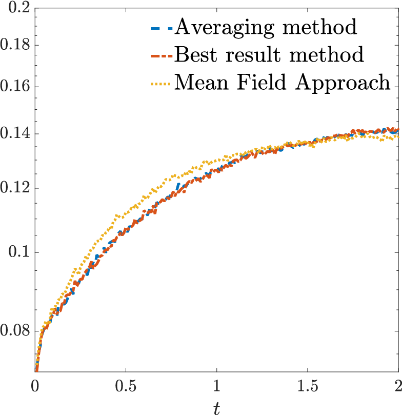
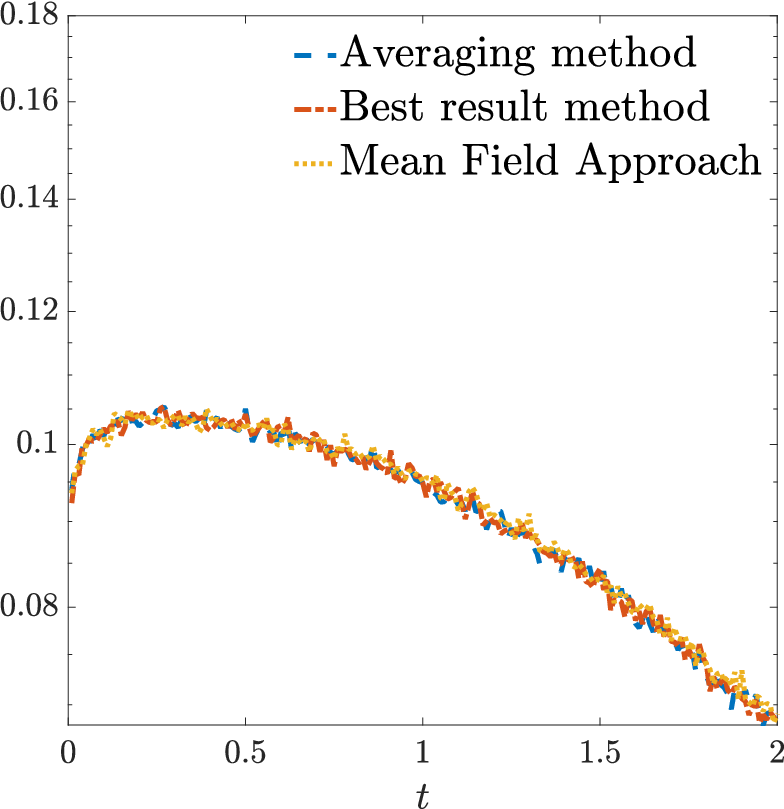
In this last one-dimensional simulation we consider a model with a Cucker–Smale-type kernel, meaning a radial kernel of the form $P(r)=(1+r^{2})^{-2}$. This interaction function models the decay of influence with increasing distance $r$ between agents, capturing the realistic weakening of influence as agents become more distant in the opinion or spatial domain. The diffusion function now depends on the relative position of the two agents interacting, specifically $D(x,y)=\widetilde{D}(x,y)(y-x)$ with $\widetilde{D}(x,y)=\widetilde{D}(\lvert x-y\rvert)=\widetilde{D}(r)=0.25/(1+r)^{2}$. The objective of this simulation is to discover $P$ and $\widetilde{D}$. We notice that in this case, both for the random batch approach and for the mean field one, the subproblem for learning the diffusion function gets modified. The dataset is composed of $10^{5}$ particles and $201$ time frames with $\Delta t=0.01$. Figure 7 shows on the left an example of the data used for the case $\ell=4$ and $M_{P}=25$, which is true for both the kernel and the diffusion reconstruction in the random batch case, only for the kernel in the mean field approach. On the right, we have the data used for problem (41) in the setting $\ell=1$, $M_{D}=20$. In the optimization problem, we set $\kappa_{P}=-1$ and $\overline{\rho}=1$ in (19). Further, in this test, instead of setting the value of the diffusion equal to zero at the boundary of the domain, we tried two different approaches: in the first, we only impose the value of the diffusion in $\lvert x-y\rvert=r=0$, obtaining the results presented in Figure 8 and in Table 4. In (20) we set $\kappa_{P}=0$ and $\overline{\zeta}_{0}=0.25$. As it is clear from the central picture in Figure 8, in this problem the averaging approach for Algorithm 1 isn’t able to reconstruct the value of the diffusion for large distances between particles. This is due to the structure of the data implied, since the large majority of the particles are close together and the probability of finding a random couple that has a distance $r\approx 2$ is low. This lack of information on far couples is what causes such strong inaccuracy for said approach for larger value of $r\in\left[0,2\right]$. Figure 9 and Table 5 show the results when monotonicity is imposed for the diffusion learning problem (in (20) we set $\kappa_{P}=-1$ and $\overline{\zeta}_{0}=0.25$). Again, as in the kernel reconstruction, it is hard for the random batch method to reconstruct the values of the diffusion when the distance between interacting particles $r$ is close to $2$, for the same reason stated before. It is worth noting that the mean-field approach overcomes this lack of information by reconstructing the density $f$ on the entire domain $[-1,1]$.

Figure 7: Test 3. Data used for the reconstruction of the kernel when $\ell=4$ and $M_{P}=25$ (left) and data used for the reconstruction of the diffusion in the mean field approach with $\ell=1$ and $M_{D}=20$ (right).

Figure 8: Test 3. Reconstruction of the kernel $P(r)=(1+r^{2})^{-2}$ using $10$ basis functions, $\mathscr{S}=3$, with approaches (34) (averaging) and (36) (best), $N_{p}=1000$, and $K=10$, compared with the mean-field method (left). Reconstruction of the density $D(x)$ using $8$ basis functions with $\mathscr{S}=2$ for the random batch approach and $\ell=1$, $M_{D}=10$ for the mean-field method (center). Comparison between the data and the reconstructed density at the final time (right).

Averaging method (Alg. 1)
$\mathscr{S}$	$E^{1}_{P}$	$E^{\infty}_{P}$	$E^{\textrm{ave}}_{f}$	$E^{\textrm{fin}}_{f}$	$E^{1}_{D}$	$E^{\infty}_{D}$
$1$	$7.94\cdot 10^{-2}$	$1.21\cdot 10^{-1}$	$3.34\cdot 10^{-3}$	$6.38\cdot 10^{-3}$	$2.97\cdot 10^{-1}$	$7.42\cdot 10^{-1}$
$2$	$7.53\cdot 10^{-2}$	$1.06\cdot 10^{-1}$	$3.35\cdot 10^{-3}$	$7.37\cdot 10^{-3}$	$3.04\cdot 10^{-1}$	$7.42\cdot 10^{-1}$
$3$	$6.78\cdot 10^{-2}$	$1.01\cdot 10^{-1}$	$2.82\cdot 10^{-3}$	$6.58\cdot 10^{-3}$	$3.88\cdot 10^{-1}$	$1.45$
Best result method (Alg. 1)
$\mathscr{S}$	$E^{1}_{P}$	$E^{\infty}_{P}$	$E^{\textrm{ave}}_{f}$	$E^{\textrm{fin}}_{f}$	$E^{1}_{D}$	$E^{\infty}_{D}$
$1$	$7.30\cdot 10^{-2}$	$1.26\cdot 10^{-1}$	$2.05\cdot 10^{-3}$	$5.63\cdot 10^{-3}$	$5.33\cdot 10^{-2}$	$1.32\cdot 10^{-1}$
$2$	$6.39\cdot 10^{-2}$	$6.16\cdot 10^{-2}$	$1.95\cdot 10^{-3}$	$4.73\cdot 10^{-3}$	$5.12\cdot 10^{-2}$	$9.25\cdot 10^{-2}$
$3$	$7.08\cdot 10^{-2}$	$1.31\cdot 10^{-1}$	$2.58\cdot 10^{-3}$	$6.04\cdot 10^{-3}$	$5.46\cdot 10^{-2}$	$6.99\cdot 10^{-2}$
Mean Field Approach (Alg. 2)
$\mathscr{S}$	$E^{1}_{P}$	$E^{\infty}_{P}$	$E^{\textrm{ave}}_{f}$	$E^{\textrm{fin}}_{f}$	$E^{1}_{D}$	$E^{\infty}_{D}$
$1$	$4.76\cdot 10^{-2}$	$4.71\cdot 10^{-2}$	$1.32\cdot 10^{-3}$	$1.79\cdot 10^{-3}$	$3.11\cdot 10^{-2}$	$3.66\cdot 10^{-2}$
$2$	$4.93\cdot 10^{-2}$	$4.85\cdot 10^{-2}$	$1.15\cdot 10^{-3}$	$1.42\cdot 10^{-3}$	$3.11\cdot 10^{-2}$	$3.66\cdot 10^{-2}$
$3$	$4.42\cdot 10^{-2}$	$4.65\cdot 10^{-2}$	$1.53\cdot 10^{-3}$	$2.15\cdot 10^{-3}$	$3.11\cdot 10^{-2}$	$3.66\cdot 10^{-2}$

Table 4: Test 3. Errors for the identification of kernel $P(r)=(1+r^{2})^{-2}$ using $10$ basis functions and diffusion $D(r)=(1+r)^{-2}$ using $8$ basis functions.

Figure 9: Test 3. Reconstruction of kernel $P(r)=((1+r^{2})^{-2}$ using $10$ basis functions, $\ell=4$ and $M_{P}=25$ using approach (34) (averaging) and (36) (best), with $N_{p}=1000$ and $K=10$, superposed with the mean field (left). Reconstruction of the density function $D(x)$ using $8$ basis functions $\ell=2$ and $M_{D}=50$ for the random batch approach and $\ell=1$ and $M_{D}=10$ for the mean field (center). Comparison between the data and the reconstructed density at the final time (right) using the reconstructed kernels and densities.

Averaging method (Alg. 1)
$\mathscr{S}$	$E^{1}_{P}$	$E^{\infty}_{P}$	$E^{\textrm{ave}}_{f}$	$E^{\textrm{fin}}_{f}$	$E^{1}_{D}$	$E^{\infty}_{D}$
$1$	$7.20\cdot 10^{-2}$	$1.21\cdot 10^{-1}$	$1.78\cdot 10^{-3}$	$3.58\cdot 10^{-3}$	$7.68\cdot 10^{-2}$	$3.33\cdot 10^{-1}$
$2$	$8.77\cdot 10^{-2}$	$1.49\cdot 10^{-1}$	$2.18\cdot 10^{-3}$	$5.86\cdot 10^{-3}$	$7.66\cdot 10^{-2}$	$3.33\cdot 10^{-1}$
$3$	$6.70\cdot 10^{-2}$	$1.26\cdot 10^{-1}$	$2.24\cdot 10^{-3}$	$5.29\cdot 10^{-3}$	$7.59\cdot 10^{-2}$	$3.33\cdot 10^{-1}$
Best result method (Alg. 1)
$\mathscr{S}$	$E^{1}_{P}$	$E^{\infty}_{P}$	$E^{\textrm{ave}}_{f}$	$E^{\textrm{fin}}_{f}$	$E^{1}_{D}$	$E^{\infty}_{D}$
$1$	$6.36\cdot 10^{-2}$	$8.54\cdot 10^{-2}$	$1.68\cdot 10^{-3}$	$5.01\cdot 10^{-3}$	$7.68\cdot 10^{-2}$	$3.33\cdot 10^{-1}$
$2$	$6.21\cdot 10^{-2}$	$8.83\cdot 10^{-2}$	$1.83\cdot 10^{-3}$	$4.69\cdot 10^{-3}$	$7.53\cdot 10^{-2}$	$3.33\cdot 10^{-1}$
$3$	$7.34\cdot 10^{-2}$	$1.10\cdot 10^{-1}$	$2.06\cdot 10^{-3}$	$5.08\cdot 10^{-3}$	$7.57\cdot 10^{-2}$	$3.33\cdot 10^{-1}$
Mean Field Approach (Alg. 2)
$\mathscr{S}$	$E^{1}_{P}$	$E^{\infty}_{P}$	$E^{\textrm{ave}}_{f}$	$E^{\textrm{fin}}_{f}$	$E^{1}_{D}$	$E^{\infty}_{D}$
$1$	$4.76\cdot 10^{-2}$	$4.71\cdot 10^{-2}$	$1.59\cdot 10^{-3}$	$1.53\cdot 10^{-3}$	$2.85\cdot 10^{-2}$	$3.71\cdot 10^{-2}$
$2$	$4.93\cdot 10^{-2}$	$4.85\cdot 10^{-2}$	$1.07\cdot 10^{-3}$	$1.57\cdot 10^{-3}$	$2.85\cdot 10^{-2}$	$3.71\cdot 10^{-2}$
$3$	$4.42\cdot 10^{-2}$	$4.65\cdot 10^{-2}$	$1.33\cdot 10^{-3}$	$1.84\cdot 10^{-3}$	$2.85\cdot 10^{-2}$	$3.71\cdot 10^{-2}$

Table 5: Test 3. Errors for the identification of kernel $P(r)=(1+r^{2})^{-2}$ using $10$ basis functions and diffusion $\tilde{D}(r)=(1+r)^{-2}$ using $8$ basis functions.

5.2 Two-dimensional examples

In this section, we provide two different two-dimensional examples. In the first one, the interaction kernel is of the attraction-repulsion type, and the diffusion is anisotropic. In the second simulation, instead, the kernel is attractive and the diffusion is nonlocal and radial. In the two dimensional case we report, instead of the errors defined in (26), we reconstruct the density through histograms, recovering both the density of the data $f^{n}(x)$ and the reconstructed one using the learned kernels, $\widehat{f}^{n}(x)$, then we compute

$$E^{1}_{f}=\frac{\sum_{n=1}^{N_{T}}\|f^{n}-\widehat{f}^{n}\|_{L^{1}([-1,1]^{2})}}{\sum_{n=1}^{N_{T}}\|f^{n}\|_{L^{1}([-1,1]^{2})}},\quad E^{1}_{f_{T}}=\frac{\|f^{N_{T}}-\widehat{f}^{N_{T}}\|_{L^{1}([-1,1]^{2})}}{\|{f}^{N_{T}}\|_{L^{1}([-1,1]^{2})}}.$$ (48)

This numerical error analysis will hold true for both presented algorithms.

Test 4: attraction-repulsion model with anisotropic diffusion

In this first two-dimensional simulation, we consider a model with the attraction-repulsion radial kernel given by $P(r)=(-(0.1+r)^{-1.15}+r^{2})/2$, with $r$ being the euclidean distance between the two bi-dimensional opinions. The density is anisotropic and it is equal to $D_{1}(x_{1})=(1-x_{1}^{2})/4$ along the first opinion $x_{1}$, while it is equal to and $D_{2}(x_{2})=\sqrt{1-x_{2}^{2}}/5$ along the second one $x_{2}$. The dataset is composed of $N=10^{5}$ agents, with $201$ available time frames for each agent, having a distance of $\Delta t=0.01$ between them. The initial condition is a uniform distribution in $\left[-0.85,0.85\right]^{2}$. In the optimization problem, we set $\kappa_{P}=1$ and $\overline{\rho}=-7$ in (19), whereas in (20) we set $\kappa_{P}=0,\,\overline{\zeta}_{0}=0=\overline{\zeta}_{N_{b}^{D}.}$ for both diffusion functions.

Figure 10 shows a visual comparison between the true kernel and the reconstructed ones using the different approaches (left), the reconstructed diffusion along the first dimension $D_{1}$ (center), and the reconstructed diffusion along the second dimension $D_{2}$ (right). Figure 11, instead, shows a comparison between the reconstructed density at the final time and plots of the errors at the final time: the top left picture shows the density at the final time using the averaging approach, the top center one using the best case approach, and the top right one shows the reconstructed density using the mean field approach. The bottom row shows the absolute value of the error on the reconstructed density (compared to the data) for the averaging (left), best case (center) and mean field approaches (right). Finally, Table 6 shows a comparison between the errors for different choices of setting $\mathscr{S}$ in the kernel reconstruction, for the three approaches. Also in this example, we can see that the discovered diffusion functions present a larger error close to the boundary but, as already mentioned in the previous tests, this is a consequence of the lack of information when $x_{1}=\pm 1$ or $x_{2}=\pm 1$. The kernel for larger $r$ also presents an error but, again, this is expected since we do not have information when the particles are not close.

Figure 10: Test 4. (Test 2D) Reconstruction of kernel $P=(-(0.1+r)^{-1.15}+r^{2})/2$ using $10$ basis functions, $\ell=2$ and $M_{P}=50$ (left), reconstruction of the density function $D_{1}(x_{1})$ using $15$ basis functions $\ell=1$ and $M_{D_{1}}=20$ (center), reconstruction of the density function $D_{2}(x_{2})$ using $15$ basis functions $\ell=1$ and $M_{D_{2}}=20$ (right).

Figure 11: Test 4. Evolution of the reconstructed density (left) and trend of the normalized $L^{1}$ errors over time for the different reconstruction strategies (right), setting $\mathscr{S}=3$.

Averaging method (Alg. 1)
$\mathscr{S}$	$E^{1}_{P}$	$E^{\infty}_{P}$	$E^{1}_{f}$	$E^{1}_{f_{T}}$
$2$	$1.83\cdot 10^{-1}$	$2.92\cdot 10^{-1}$	$1.21\cdot 10^{-1}$	$1.42\cdot 10^{-1}$
$3$	$2.30\cdot 10^{-1}$	$2.52\cdot 10^{-1}$	$1.19\cdot 10^{-1}$	$1.41\cdot 10^{-1}$
Best result method (Alg. 1)
$\mathscr{S}$	$E^{1}_{P}$	$E^{\infty}_{P}$	$E^{1}_{f}$	$E^{1}_{f_{T}}$
$1$	$4.06\cdot 10^{-1}$	$3.19\cdot 10^{-1}$	$8.83\cdot 10^{-2}$	$9.22\cdot 10^{-2}$
$2$	$2.06\cdot 10^{-1}$	$2.97\cdot 10^{-1}$	$1.20\cdot 10^{-1}$	$1.43\cdot 10^{-1}$
$3$	$2.13\cdot 10^{-1}$	$3.11\cdot 10^{-1}$	$1.19\cdot 10^{-1}$	$1.42\cdot 10^{-1}$
Mean Field Approach (Alg. 2)
$\mathscr{S}$	$E^{1}_{P}$	$E^{\infty}_{P}$	$E^{1}_{f}$	$E^{1}_{f_{T}}$
$1$	$1.67\cdot 10^{-1}$	$1.47\cdot 10^{-1}$	$1.24\cdot 10^{-1}$	$1.41\cdot 10^{-1}$
$2$	$1.66\cdot 10^{-1}$	$1.47\cdot 10^{-1}$	$1.23\cdot 10^{-1}$	$1.40\cdot 10^{-1}$
$3$	$1.62\cdot 10^{-1}$	$1.47\cdot 10^{-1}$	$1.21\cdot 10^{-1}$	$1.37\cdot 10^{-1}$

Table 6: Test 4. Errors for the identification of kernel $P=(-(0.1+r)^{-1.15}+r^{2})/2$ using $10$ basis functions. The errors on the diffusion along the first variable are $E^{1}_{D_{1}}=4.40\cdot 10^{-2}$ and $E^{\infty}_{D_{1}}=1.11\cdot 10^{-2}$, while the errors on the diffusion along the second variable are $E^{1}_{D_{2}}=3.47\cdot 10^{-2}$ and $E^{\infty}_{D_{1}}=9.82\cdot 10^{-2}$.

Test 5: non-local radial density in the two-dimensional setting

This last simulation is in a two-dimensional setting, with a bounded confidence attractive radial kernel given by $P(r)=\chi(r<1)$ and a nonlocal diffusion $D(x,y)=\tilde{D}(x,y)(y-x)$, with $\tilde{D}(x,y)=\tilde{D}(\lvert x-y\rvert)=\tilde{D}(r)=(1+r^{2})^{-2}$. With this choice of interaction and diffusion functions the dynamics is attractive, so starting from a uniform distribution of the agents we witness their concentration around $(0,0)$ over time. The objective is to reconstruct both $P$ and $\tilde{D}$, as in Test 4. The available dataset consists in the collection of two opinions of $N=10^{5}$ agents, with $201$ available data frames for each of the two opinions, and a time step $\Delta t=0.01$ between two consecutive time frames. Unfortunately, with the hardware at our disposal, we were unable to perform simulations using the averaging approach in the case $\ell=1$, $M_{P}=M_{D}=100$ and $\ell=2$, $M_{P}=M_{D}=50$. We report the qualitative results for the case $\ell=4$ and $M_{P}=25$ in Figures 12 and 13. For the optimization problem, we set $\kappa_{P}=-1$ and $\overline{\rho}=1$ in (19), whereas in (20) we set $\kappa_{D}=-1$ and $\overline{\zeta}_{0}=1$.

Figure 12: Test 5. (Test 2D) Reconstruction of kernel $P=\chi(r<1)$ using $N_{b}^{P}=21$, $\ell=4$ and $M_{P}=25$ (left), reconstruction of the density function $\tilde{D}(r)$ using $N_{b}^{D}=10$, $\ell=4$ and $M_{D_{2}}=25$ (right).

Figure 13: Test 5. Evolution of the reconstructed density (left) and trend of the normalized $L^{1}$ errors over time for the different reconstruction strategies (right), setting $\mathscr{S}=3$.

6 Conclusions

In this work, we proposed a data-driven framework for the identification of interaction kernels in stochastic multi-agent systems from trajectory data, addressing the challenging setting in which the pairwise interactions between agents are not directly observable. Starting from a microscopic binary-interaction model, we formulated the reconstruction of both drift and diffusion terms as regression problems on suitable finite-dimensional approximation spaces. The lack of direct information on the interaction structure is handled through two complementary strategies. The first approach combines binary interactions with random batch sampling, providing an efficient approximation of the microscopic dynamics. The second approach relies on a mean-field description of the system, where the interaction kernels are inferred from the empirical particle density. In addition, we derived an a-priori error estimate for the reconstructed trajectories, showing stability of the learned dynamics and consistency of the reconstruction under suitable assumptions. Numerical experiments in one and two spatial dimensions confirm the effectiveness of the proposed methodology. In particular, both approaches yield reconstructions with comparable accuracy, even when the interaction structure is only partially observed. This highlights the robustness of the framework with respect to incomplete information on the underlying interactions. Future research directions include the validation of the proposed methodology on real-world datasets, such as biological or social collective dynamics, as well as the use of neural-network-based representations for the interaction kernels, which may provide a more flexible approximation framework when the interaction laws depend on higher-dimensional variables or exhibit complex structures that are difficult to capture with fixed basis expansions.

Appendix A (Proof of Theorem 4.1)

Let us first observe that $\delta_{P},\,\delta_{D}$, $P_{\max},\widehat{P}_{\max}$ and $D_{\max},\widehat{D}_{\max}$ are all finite positive constants due to the fact that $\mathbf{P},\,\mathbf{D},\,\widehat{\mathbf{P}}$ and $\widehat{\mathbf{D}}$ are all continuous functions defined on a compact subset of $\mathbb{R}_{+}$. Moreover, in what follows we will make use of the elementary bounds

$$\|S-S^{\prime}\|_{2}\leq 2,\qquad S,S^{\prime}\qquad\textrm{permuation matrices}$$ (49a)

$$\|a\odot b\|_{2}^{2}\leq\|a\|_{\infty}^{2}\|b\|^{2}_{2},\qquad a,b\in\mathbb{R}^{d},$$ (49b)

Estimate for $\bar{e}^{n}$

Subtracting (44) from (42), we obtain

$$\bar{e}^{n+1}=\bar{e}^{n}+\Delta t\,A^{n}+\sqrt{\Delta t}\,B^{n}\odot\Xi^{n},$$

where

$$A^{n} :={\mathbf{P}}(R^{n})\odot\bigl(\mathsf{S}^{n}X^{n}-X^{n}\bigr)-\widehat{\mathbf{P}}(\bar{R}^{n})\odot\bigl(\mathsf{S}^{n}\bar{X}^{n}-\bar{X}^{n}\bigr),$$ (50)

$$B^{n} :=\mathbf{D}(R^{n})-\widehat{\mathbf{D}}(\bar{R}^{n}).$$ (51)

Therefore, we have

$$\mathbb{E}\left[\|\bar{e}^{n+1}\|^{2}_{2}\right]= \mathbb{E}\left[\|\bar{e}^{n}\|^{2}_{2}\right]+\Delta t^{2}\mathbb{E}\left[\|A^{n}\|^{2}_{2}\right]+\Delta t\mathbb{E}\left[\|B^{n}\odot\Xi^{n}\|_{2}^{2}\right]+$$ (52)

$$\qquad 2\Delta t\mathbb{E}\left[\langle\bar{e}^{n},A^{n}\rangle\right]+2\Delta t^{3/2}\mathbb{E}\left[\langle\bar{e}^{n}+\Delta tA^{n},B^{n}\odot\Xi^{n}\rangle\right],$$

where the last term vanishes since $\Xi^{n}$ is centered. We first estimate the drift contribution. Adding and subtracting ${\mathbf{P}}(R^{n})\odot(S^{n}\bar{X}^{n}-\bar{X}^{n})$, we write $A^{n}$ as

$$A^{n}={\mathbf{P}}(R^{n})\odot\bigl((\mathsf{S}^{n}-\mathsf{I}_{N_{d}})\bar{e}^{n}\bigl)+\bigl(\mathbf{P}(R^{n})-\widehat{\mathbf{P}}(\bar{R}^{n})\bigr)\odot\bigl(\mathsf{S}^{n}\bar{X}^{n}-\bar{X}^{n}\bigr).$$ (53)

Hence, by using (49a) and the bounds (46) we have

$$\|A^{n}\|^{2}_{2} \leq 2{P}^{2}_{\textrm{max}}\|(\mathsf{S}^{n}-\mathsf{I}_{N_{d}})\bar{e}^{n}\|_{2}^{2}+2\|\bigl(\mathbf{P}(R^{n})-\widehat{\mathbf{P}}(\bar{R}^{n})\bigr)\|_{\infty}^{2}\|\bigl(\mathsf{S}^{n}\bar{X}^{n}-\bar{X}^{n}\bigr)\|^{2}_{2}$$ (54)

$$\qquad\leq 8{P}^{2}_{\textrm{max}}\|\bar{e}^{n}\|_{2}^{2}+8L^{2}\|\bigl(\mathbf{P}(R^{n})-\widehat{\mathbf{P}}(\bar{R}^{n})\bigr)\|_{\infty}^{2}$$ (55)

$$\qquad\quad\leq 8{P}^{2}_{\textrm{max}}\|\bar{e}^{n}\|_{2}^{2}+16L^{2}N_{d}\delta^{2}_{P}+64L^{2}L^{2}_{P}N_{d}\|\bar{e}^{n}\|^{2}_{2},$$ (56)

with $\mathsf{I}_{N_{d}}$ the $N_{d}\times N_{d}$ identity matrix, and where in the last inequality we added and subtracted $\widehat{\mathbf{P}}(R^{n})$ and used (46), along with Lipschitz bound for $P$. For the third term in (52), we use (49) and observe that $\|\Xi^{n}\|_{2}^{2}\sim\chi^{2}_{N_{d}}$, which implies that $\mathbb{E}\!\left[\|\Xi^{n}\|_{2}^{2}\right]=N_{d}$. Then we have

$$\mathbb{E}\left[\|B^{n}\odot\Xi^{n}\|^{2}_{2}\right] \leq\mathbb{E}\left[\|\Xi^{n}\|_{2}^{2}\right]\|(\mathbf{D}(R^{n})-\widehat{\mathbf{D}}(\bar{R}^{n}))\|^{2}_{\infty}$$ (57)

$$\qquad\leq 2N_{d}\left(4L_{D}^{2}\|\bar{e}^{n}\|_{2}^{2}+\delta_{D}^{2}\right),$$

where the last inequality is obtained by summing and subtracting ${\mathbf{D}}(\bar{R}^{n})$, and recalling the usual bounds. Finally, we estimate the fourth term on the right-hand side of (52). Using the definition of $A^{n}$ in (50), we decompose the inner product $2\langle\bar{e}^{n},A^{n}\rangle$ into two terms. The first contribution is estimated as follows

$$2\langle\bar{e}^{n},\mathbf{P}(R^{n})\odot\bigl((\mathsf{S}^{n}-\mathsf{I}_{N_{d}})\bar{e}_{n}\bigr)\rangle\leq 2\|\bar{e}^{n}\|_{2}\|(\mathsf{S}^{n}-\mathsf{I}_{N_{d}})\bar{e}_{n}\|_{2}\leq 4P_{\max}\|\bar{e}^{n}\|_{2}^{2},$$

where the last inequality follows from Cauchy-Schwarz. The second contribution can be bounded as follows, again using Cauchy-Schwarz and Young’s inequalities

$$2\langle\bar{e}^{n},\bigl(\mathbf{P}(R^{n})-\mathbf{\widehat{P}}(\bar{R}^{n})\bigr)\odot\bigl((\mathsf{S}^{n}-\mathsf{I}_{N_{d}})\bar{X}^{n}\bigl)\rangle$$ (58)

$$\quad\leq 2\|\bar{e}^{n}\|_{2}\|\bigl(\mathbf{P}(R^{n})-\mathbf{\widehat{P}}(\bar{R}^{n})\bigr)\|_{2}\|(\mathsf{S}^{n}-\mathsf{I}_{N_{d}})\bar{X}^{n}\|_{\infty}$$ (59)

$$\qquad\leq 4L\|\bar{e}^{n}\|_{2}\left(\delta_{P}\sqrt{N_{d}}+2L_{P}\|\bar{e}^{n}\|_{2}\right)\leq 4L^{2}\delta_{P}^{2}N_{d}+\left(1+4LL_{P}\right)\|\bar{e}^{n}\|_{2}^{2}$$ (60)

Then, from (52), setting $\bar{E}^{2}_{n}:=\mathbb{E}[\|\bar{e}^{n}\|^{2}_{2}]$, and combining the previous estimates, we have

$$\bar{E}^{2}_{n+1}\leq \bar{E}^{2}_{n}+8\Delta t^{2}\left[\bigl(P_{\max}^{2}+8L^{2}L_{P}^{2}\bigr)\bar{E}^{2}_{n}+2L^{2}N_{d}\delta_{P}^{2}\right]+$$

$$\Delta t\left[(1+4LL_{P}+4P_{\max}+8N_{d}L^{2}_{D})\bar{E}^{2}_{n}+2L^{2}N_{d}\delta_{P}^{2}+2N_{d}\delta_{D}^{2}\right],$$

Furthermore, since $\Delta t\leq 1$, $\Delta t^{2}$ terms can be absorbed into the $\Delta t$ contribution, as follows

$$\bar{E}^{2}_{n+1}\leq(1+C_{1}\Delta t)\bar{E}^{2}_{n}+C_{2}(\delta_{P}^{2}+\delta_{D}^{2})\Delta t,$$

where $C_{1}:=8P_{\max}^{2}+64L^{2}L_{P}^{2}+4P_{\max}+4LL_{P}+8N_{d}L_{D}^{2}+1$, and $C_{2}:=18L^{2}N_{d}+2N_{d}.$ Iterating this process, since we assumed $\bar{E}^{2}_{0}=0$, it follows that

$$\bar{E}^{2}_{n}\leq\frac{C_{2}}{C_{1}}(\delta_{P}^{2}+\delta_{D}^{2})\Bigl((1+C_{1}\Delta t)^{n}-1\Bigr)\leq\frac{C_{2}}{C_{1}}(\delta_{P}^{2}+\delta_{D}^{2})\left(e^{C_{1}T}-1\right).$$ (61)

Estimate for $\widetilde{e}^{n}$

We consider now the error term given by

$$\widetilde{e}^{n+1}=\widetilde{e}^{n}+\Delta t\,\widetilde{A}^{n}+\sqrt{\Delta t}\,\widetilde{B}^{n}\odot\Xi^{n},$$

where now

$$\widetilde{A}^{n} :=\widehat{{\mathbf{P}}}(\bar{R}^{n})\odot\bigl({\mathsf{S}}^{n}\bar{X}^{n}-\bar{X}^{n}\bigr)-\widehat{\mathbf{P}}(\widetilde{R}^{n})\odot\bigl(\widehat{\mathsf{S}}^{n}\widetilde{X}^{n}-\widetilde{X}^{n}\bigr)$$

$$\widetilde{B}^{n} :=\widehat{\mathbf{D}}(\bar{R}^{n})\odot\Xi^{n}-\widehat{\mathbf{D}}(\widetilde{R}^{n})\odot\widehat{\Xi}^{n}.$$

Analogously to (52) we can expand the norm $\|\widetilde{e}^{n+1}\|^{2}_{2}$ and control the different terms. Following the previous computation, for $\|\widetilde{A}^{n}\|^{2}_{2}$ we have

$$\|\widetilde{A}^{n}\|_{2}^{2}\leq 2\|\bigl(\widehat{\mathbf{P}}(\bar{R}^{n})-\widehat{\mathbf{P}}(\widetilde{R}^{n})\bigr)\odot\bigl(\mathsf{S}^{n}\bar{X}^{n}-\bar{X}^{n}\bigr)\|^{2}_{2}$$ (62)

$$\qquad+2\|\widehat{\mathbf{P}}(\widetilde{R}^{n})\odot\bigl(\mathsf{S}^{n}\bar{X}^{n}-\widehat{\mathsf{S}}^{n}\widetilde{X}^{n}-\widetilde{e}^{n}\bigr)\|_{2}^{2},$$

where, for the first term, using Lipschitz continuity of $\widehat{\mathbf{P}}$, the bounds (46) and (49b) we have

$$2\|\bigl(\widehat{\mathbf{P}}(\bar{R}^{n})-\widehat{\mathbf{P}}(\widetilde{R}^{n})\bigr)\odot\bigl(\mathsf{S}^{n}\bar{X}^{n}-\bar{X}^{n}\bigr)\|^{2}_{2}\leq 2\|\widehat{\mathbf{P}}(\bar{R}^{n})-\widehat{\mathbf{P}}(\widetilde{R}^{n})\|_{\infty}^{2}\|\bigl(\mathsf{S}^{n}-I_{N_{d}}\bigr)X^{n}\|_{2}^{2}$$

$$\qquad\leq 8L^{2}N_{d}L^{2}_{\widehat{P}}\|(\mathsf{S}^{n}-\widehat{\mathsf{S}}^{n})\bar{X}^{n}+(\widehat{\mathsf{S}}^{n}-I_{N_{d}})\widetilde{e}^{n})\|_{2}^{2}\leq 16L^{2}L^{2}_{\widehat{P}}N_{d}(\eta_{S}^{2}N_{d}L^{2}+4\|\widetilde{e}^{n}\|^{2}_{2}).$$

The estimate for the second term follows similarly retaining the bound on $\widehat{P}$ as follows

$$2\|\widehat{\mathbf{P}}(\widetilde{R}^{n})\odot\bigl(\mathsf{S}^{n}\bar{X}^{n}-\widehat{\mathsf{S}}^{n}\widetilde{X}^{n}-\widetilde{e}^{n}\bigr)\|_{2}^{2}\leq 4\widehat{P}_{\textrm{max}}^{2}\left(\eta^{2}_{S}N_{d}L^{2}+4\|\widetilde{e}^{n}\|_{2}^{2}\right)$$

For the term $\widetilde{B}^{n}$, proceeding as in (57) and using the Lipschitz continuity of $\widehat{D}$ together with the bounds (46), we obtain

$$\mathbb{E}\left[\|\widetilde{B}^{n}\|^{2}_{2}\right]\leq \mathbb{E}\left[\|\Xi^{n}\|_{2}^{2}\right]\|\bigl(\widehat{\mathbf{D}}(\bar{R}^{n})-\widehat{\mathbf{D}}(\widetilde{R}^{n})\bigr)\|_{\infty}^{2}$$ (63)

$$\quad\leq 2N_{d}L^{2}_{\widehat{D}}(\eta_{S}^{2}N_{d}L^{2}+4\|\widetilde{e}^{n}\|^{2}_{2})$$

Finally, the mixed term appearing in the expansion of the error $\|\widetilde{e}^{n+1}\|^{2}_{2}$ reads

$$2\langle\widetilde{e}^{n},\widetilde{A}^{n}\rangle= 2\langle\widetilde{e}^{n},\bigl(\widehat{\mathbf{P}}(\bar{R}^{n})-\widehat{\mathbf{P}}(\widetilde{R}^{n})\bigr)\odot\bigl(\mathsf{S}^{n}\bar{X}^{n}-\bar{X}^{n}\bigr)\rangle+$$ (64)

$$\qquad 2\langle\widetilde{e}^{n},\widehat{\mathbf{P}}(\widetilde{R}^{n})\odot\bigl(\mathsf{S}^{n}\bar{X}^{n}-\widehat{\mathsf{S}}^{n}\widetilde{X}^{n}-\widetilde{e}^{n}\bigr)\rangle.$$

Here, using (49b) and Cauchy-Schwarz in the first term of the right hand side we obtain

$$2\langle\widetilde{e}^{n},\bigl(\widehat{\mathbf{P}}(\bar{R}^{n})-\widehat{\mathbf{P}}(\widetilde{R}^{n})\bigr)\odot\bigl(\mathsf{S}^{n}\bar{X}^{n}-\bar{X}^{n}\bigr)\rangle$$

$$\quad\leq 2\|\widetilde{e}^{n}\|_{2}\|\widehat{\mathbf{P}}(\bar{R}^{n})-\widehat{\mathbf{P}}(\widetilde{R}^{n})\|_{2}\|\mathsf{S}^{n}\bar{X}^{n}-\bar{X}^{n}\|_{\infty}\leq 4LL_{\widehat{P}}\|\widetilde{e}^{n}\|_{2}(\eta_{S}L\sqrt{N_{d}}+2\|\widetilde{e}^{n}\|_{2}),$$

and similarly for the second term

$$2\langle\widetilde{e}^{n},\widehat{\mathbf{P}}(\widetilde{R}^{n})\odot\bigl(\mathsf{S}^{n}\bar{X}^{n}-\widehat{\mathsf{S}}^{n}\widetilde{X}^{n}-\widetilde{e}^{n}\bigr)\rangle$$

$$\quad\leq 2\|\widetilde{e}^{n}\|_{2}\|\widehat{\mathbf{P}}(\widetilde{R}^{n})\|_{\infty}\|\bigl(\mathsf{S}^{n}\bar{X}^{n}-\widehat{\mathsf{S}}^{n}\widetilde{X}^{n}-\widetilde{e}^{n}\bigr)\|_{2}\leq 2\widehat{P}_{\max}\|\widetilde{e}^{n}\|_{2}(\eta_{S}L\sqrt{N_{d}}+2\|\widetilde{e}^{n}\|_{2}).$$

Then combining this two estimate and using Young’s inequality we have

$$2\langle\widetilde{e}^{n},\widetilde{A}^{n}\rangle \leq 4(\widehat{P}_{\max}+2LL_{\widehat{P}})\|\widetilde{e}^{n}\|^{2}_{2}+2(\widehat{P}_{\max}+2LL_{\widehat{P}})\eta_{S}\sqrt{N_{d}}L\|\widetilde{e}^{n}\|_{2}$$

$$\quad\leq(1+4(\widehat{P}_{\max}+2LL_{\widehat{P}}))\|\widetilde{e}^{n}\|^{2}_{2}+(\widehat{P}_{\max}+2LL_{\widehat{P}})^{2}L^{2}N_{d}\eta_{S}^{2}.$$

Setting $\widetilde{E}^{2}_{n}:=\mathbb{E}\!\left[\|\widetilde{e}^{n}\|_{2}^{2}\right]$, and combining the previous estimates, we obtain a recursive bound for $\widetilde{E}^{2}_{n}$ as

$$\widetilde{E}^{2}_{n+1}\leq\bigl(1+\Delta tC_{3}\bigr)\widetilde{E}^{2}_{n}+\Delta tC_{4}\eta^{2}_{S},$$

where the constants are $C_{3}:=1+4\widehat{P}_{\max}+2LL_{\widehat{P}}+8N_{d}L^{2}_{\widehat{D}}+8\widehat{P}^{2}_{\max}+64L^{2}L^{2}_{\widehat{P}}N_{d})$ and $C_{4}:=(\widehat{P}_{\max}+2LL_{\widehat{P}})^{2}N_{d}+2N_{d}^{2}L_{\widehat{D}}^{2}L^{2}+4\widehat{P}_{\max}^{2}N_{d}L^{2}+16L^{4}L^{2}_{\widehat{P}}N^{2}_{d}$. Here we used the assumption $\Delta t\leq 1$, which implies $\Delta t^{2}\leq\Delta t$; consequently, all terms of order $\Delta t^{2}$ can be absorbed into the constants multiplying $\Delta t$. Eventually, recalling that $\widetilde{E}^{2}_{0}=0$ this leads to

$$\widetilde{E}^{2}_{n+1}\leq\frac{C_{4}\eta_{S}^{2}}{C_{3}}\left((1+\Delta tC_{3})^{n}-1\right)\leq\frac{C_{4}\eta_{S}^{2}}{C_{3}}\left(e^{C_{3}T}-1\right)$$ (65)

Combining (61) and (65) we finally get

$$\mathbb{E}\left[\|e^{n+1}\|_{2}^{2}\right]\leq\widehat{C}_{2}(\delta_{P}^{2}+\delta_{D}^{2}+\eta_{S}^{2})\left(\exp\left\{\widehat{C}_{1}T\right\}-1\right),$$

for all $n=0,\dots,M-1$, with $\widehat{C_{2}}=\max\left\{C_{2}/{C_{1}},{C_{4}}/{C_{3}}\right\}$ and $\widehat{C}_{1}=\max\left\{C_{1},\,C_{3}\right\}$.

References

- [1] (2014) Boltzmann-type control of opinion consensus through leaders. Philosophical Transactions of the Royal Society A 372, pp. 20140138. Cited by: §1.
- [2] (2025) A data-driven kinetic model for opinion dynamics with social network contacts. European Journal of Applied Mathematics 36 (2), pp. 264–290. Cited by: §1.
- [3] (2013) Binary interaction algorithms for the simulation of flocking and swarming dynamics. Multiscale Modeling & Simulation 11 (1), pp. 1–29. Cited by: §1.
- [4] (2025) Computation and control of unstable steady states for mean field multiagent systems. Proceedings of the Royal Society A: Mathematical, Physical and Engineering Sciences 481 (2311). Cited by: §1.
- [5] (1997) Self-organization in social insects. Trends in Ecology & Evolution 12, pp. 188–193. Cited by: §1.
- [6] (2023) Data-driven entropic spatially inhomogeneous evolutionary games. European Journal of Applied Mathematics 34 (1), pp. 106–159. Cited by: §1.
- [7] (2017) Inferring interaction rules from observations of evolutive systems I: the variational approach. Mathematical Models and Methods in Applied Sciences 27 (05), pp. 909–951. Cited by: §1, §1, §3.
- [8] (2025) Wasserstein convergence rates for stochastic particle approximation of Boltzmann models. arXiv preprint arXiv:2504.10091. Cited by: §1.
- [9] (2016) Discovering governing equations from data by sparse identification of nonlinear dynamical systems. Proceedings of the National Academy of Sciences of the United States of America, 115, pp. 3932–3937. Cited by: §1.
- [10] (2010) Asymptotic flocking dynamics for the kinetic Cucker–Smale model. SIAM Journal on Mathematical Analysis 42, pp. 218–236. Cited by: §1.
- [11] (2019) Particle based gPC methods for mean-field models of swarming with uncertainty. Communications in Computational Physics 25 (2), pp. 508–531. Cited by: §1.
- [12] (2014) The derivation of swarming models: mean-field limit and Wasserstein distances. In Collective Dynamics from Bacteria to Crowds, CISM Courses and Lectures, Vol. 553, pp. 1–46. Cited by: §1.
- [13] (2025) Sparse identification of nonlocal interaction kernels in nonlinear gradient flow equations via partial inversion. Mathematical Models and Methods in Applied Sciences 35 (05), pp. 1073–1131. Cited by: §1.
- [14] (2005) Effective leadership and decision-making in animal groups on the move. Nature 433 (7025), pp. 513–516. External Links: Document Cited by: §1.
- [15] (2026) Augmented data and neural networks for robust epidemic forecasting: application to COVID-19 in italy. Mathematical Biosciences and Engineering 23 (2), pp. 474–498. External Links: ISSN 1551-0018, Document Cited by: §1.
- [16] (2021) Kinetic models for epidemic dynamics with social heterogeneity. Journal of Mathematical Biology 83 (4), pp. 4. External Links: Document Cited by: §1.
- [17] (2009) Boltzmann and Fokker–Planck equations modelling opinion formation in the presence of strong leaders. Proceedings of the Royal Society A: Mathematical, Physical and Engineering Sciences 465 (2112), pp. 3687–3708. Cited by: §1.
- [18] (2016) A Cucker–Smale model with noise and delay. SIAM Journal on Applied Mathematics 76 (4), pp. 1535–1557. Cited by: §1.
- [19] (2021) Learning interaction kernels in heterogeneous systems of agents from multiple trajectories. Journ. Mach. Learn. Res. 2, pp. 1–67. Cited by: §1, §3, §5.
- [20] (2025) Recent kernel methods for interacting particle systems: first numerical results. European Journal of Applied Mathematics 36 (2), pp. 464–489. Cited by: §1.
- [21] (2005) Nonlinear Fokker-Planck equations: fundamentals and applications. Springer. Cited by: §2.1.
- [22] (2025) Mean field error estimate of the random batch method for large interacting particle system. ESAIM: Mathematical Modelling and Numerical Analysis 59 (1), pp. 265–289. Cited by: §1.
- [23] (2020) Random batch methods (RBM) for interacting particle systems. Journal of Computational Physics 400, pp. 108877. Cited by: §1.
- [24] (2021-06) Physics-informed machine learning. Nature Reviews Physics 3 (6), pp. 422–440. External Links: Document, ISSN 2522-5820 Cited by: §1.
- [25] (2022) Learning interaction kernels in mean-field equations of first-order systems of interacting particles. SIAM Journal on Scientific Computing 44 (1), pp. A260–A285. Cited by: §1.
- [26] (2022) Learning interaction kernels in stochastic systems of interacting particles from multiple trajectories. Found. Comput. Math. 22 (4), pp. 1013–1067. External Links: ISSN 1615-3375,1615-3383, MathReview Entry Cited by: §1, §3.
- [27] (2019) Nonparametric inference of interaction laws in systems of agents from trajectory data. Proceedings of the National Academy of Sciences 116 (29), pp. 14424–14433. Cited by: §1.
- [28] (2021) Weak SINDy for partial differential equations. Journal of Computational Physics 443, pp. 110525. Cited by: §1.
- [29] (2023) Learning theory for inferring interaction kernels in second-order interacting agent systems. Sampling Theory, Signal Processing and Data Analysis. Cited by: §1, §1.
- [30] (1980) Direct simulation scheme derived from the Boltzmann equation. I. Monocomponent gases. Journal of the Physical Society of Japan 49 (5), pp. 2042–2049. Cited by: §1.
- [31] (2006) Numerical optimization. Cited by: §3.1.
- [32] (2013) Interacting multiagent systems: kinetic equations and Monte Carlo methods. OUP Oxford. Cited by: §1, §2.2, §2.2.
- [33] (2022) Mean-field control variate methods for kinetic equations with uncertainties and applications to socioeconomic sciences. International Journal for Uncertainty Quantification 12 (1). Cited by: §1.
- [34] (2019) Physics-informed neural networks: a deep learning framework for solving forward and inverse problems involving nonlinear partial differential equations. Journal of Computational Physics 378, pp. 686–707. External Links: ISSN 0021-9991, Document Cited by: §1.
- [35] (2017) Data-driven discovery of partial differential equations. Science Advances 3. External Links: Document Cited by: §1.
- [36] (2019) Data-driven identification of parametric partial differential equations. SIAM Journal on Applied Dynamical Systems 18 (2), pp. 643–660. External Links: Document Cited by: §1.
- [37] (2006) Kinetic models of opinion formation. Commun. Math. Sci. 4 (1), pp. 481–496. Cited by: §1, §2.2, §2.2.
- [38] (2018) Boltzmann-type models with uncertain binary interactions. Communications in Mathematical Sciences 16 (4), pp. 963–985. Cited by: §1.
- [39] (2024) On higher order drift and diffusion estimates for stochastic SINDy. SIAM Journal on Applied Dynamical Systems 23 (2), pp. 1504–1539. Cited by: §1.