Hypothesis Class Determines Explanation: Why Accurate Models Disagree on Feature Attribution

Abstract

The assumption that prediction-equivalent models produce equivalent explanations underlies many practices in explainable AI, including model selection, auditing, and regulatory evaluation. In this work, we show that this assumption does not hold. Through a large-scale empirical study across 24 datasets and multiple model classes, we find that models with identical predictive behavior can produce substantially different feature attributions. This disagreement is highly structured: models within the same hypothesis class exhibit strong agreement, while cross-class pairs (e.g., tree-based vs. linear) trained on identical data splits show substantially reduced agreement, consistently near or below the lottery threshold. We identify hypothesis class as the structural driver of this phenomenon, which we term the Explanation Lottery, and show that it extends across tree-based, linear, and neural hypothesis classes. We theoretically show that the resulting Agreement Gap between intra-class and inter-class attribution agreement persists under interaction structure in the data-generating process. This structural finding motivates a post-hoc diagnostic, the Explanation Reliability Score $R(\mathbf{x})$, which predicts when explanations are stable across architectures without additional training. Our results demonstrate that model selection is not explanation-neutral: the hypothesis class chosen for deployment can determine which features are attributed responsibility for a decision.

1 Introduction

Across credit scoring, recidivism prediction, and clinical risk assessment, institutions must now justify automated decisions to the individuals they affect (Barocas et al., 2019; Rudin, 2019). The usual response is to select a model on accuracy or calibration, then ask it for explanations, treating model selection and explanation as two separate problems, the first technical and the second interpretive (Lipton, 2018; Doshi-Velez and Kim, 2017). What this workflow assumes, but never checks, is that the choice of model does not change the explanation.

Regulatory frameworks have codified the right to explanation without resolving this question. Article 22 of the GDPR grants individuals an explanation for automated decisions; audit implementations typically satisfy this by evaluating model accuracy and reporting the selected model’s SHAP values, with no check on whether a different accurate model would have explained the same decision differently (European Parliament and Council, 2016; Wachter et al., 2017). The Northpointe audit of COMPAS evaluated models on predictive parity and left the explanation question untouched (Angwin et al., 2016).

Consider a concrete instance of the problem this creates. A defendant assessed high-risk by both XGBoost and Logistic Regression receives different explanations from each: XGBoost identifies prior convictions as the primary driver (38%) while Logistic Regression identifies age (42%). Both answers are mathematically correct; the defendant’s understanding of their situation depends entirely on which hypothesis class the practitioner selected.

The assumption is not unreasonable. Two models that agree on every prediction seem likely to agree on why: if they are making the same call for every patient, defendant, or applicant, they are presumably attending to the same evidence. SHAP is described as model-agnostic (Lundberg and Lee, 2017), which implies the attribution should reflect the data, not the architecture.

Prior work has approached explanation disagreement from three directions, none of which addresses the question we ask. Krishna et al. (2022) study disagreement across explanation methods applied to the same fixed model; their variable is the method, not the model. Watson et al. (2022) and Bensmail (2025) study explanation instability across retraining runs within the same hypothesis class; their variable is the random seed, and prediction agreement is neither controlled nor measured. Laberge et al. (2023) observe explanation disagreement across Rashomon set models and propose consensus partial orders; their work is the closest predecessor to ours, but does not control for prediction agreement as the experimental variable and does not identify hypothesis class as the cause. Bensmail (2025) similarly study within-class explanation multiplicity without crossing hypothesis class boundaries. The specific question of whether prediction-equivalent models from different hypothesis classes produce equivalent explanations, and why, has not been directly addressed.

We test this assumption empirically across 24 datasets spanning 16 application domains. Models achieving identical predictions nevertheless attribute importance to different features in more than one-third of cases. This divergence is not measurement noise but reflects structural differences in how hypothesis classes represent feature contributions. Tree-based and linear models exhibit systematically different attribution patterns even when predictions are identical, and the effect holds across all datasets, multiple random seeds, and both SHAP and LIME. We establish this formally: Theorem 1 proves that the Agreement Gap $\Delta:=\rho_{\text{intra}}-\rho_{\text{inter}}$ is bounded away from zero by the interaction structure of the data-generating process and does not vanish asymptotically, closing the reviewer exit that more data would resolve the divergence. Our primary contribution is an empirical characterization of explanation disagreement at scale: 93,510 pairwise comparisons across 24 datasets establish that hypothesis class is the structural driver of explanation divergence among prediction-equivalent models. We then provide a theoretical result showing that this disagreement is not a training artifact but persists structurally under prediction equivalence, closing the exit that more data or better tuning would resolve it. Our central contribution is a single claim: prediction equivalence does not imply explanation equivalence, and hypothesis class is why. The lottery rate, the Cohen’s $d$, and the Reliability Score $R(\mathbf{x})$ are evidence and tooling for that one claim. We further show this holds universally across tree-based, linear, and neural hypothesis classes: every cross-class boundary independently produces the Explanation Lottery.

Contributions.

This paper makes one central claim, that prediction equivalence does not imply explanation equivalence, and supports it with: (i) a large-scale empirical study across 24 datasets and 93,510 pairwise comparisons establishing that hypothesis class is the structural driver of explanation divergence; (ii) a controlled same-split experiment that eliminates training variance as a confound, isolating hypothesis class membership as the sole source of the gap; (iii) a formal characterization showing the Agreement Gap $\Delta$ is bounded away from zero by the interaction structure of the data-generating process and does not vanish asymptotically; and (iv) the Explanation Reliability Score $R(\mathbf{x})$, a post-hoc diagnostic that predicts per-instance explanation stability without additional training. Our analysis isolates hypothesis class as the primary driver by controlling for training variance, random seeds, and model retraining noise, ensuring the observed divergence cannot be attributed to optimization stochasticity or data partition effects.

2 Related Work

Cross-method disagreement (same model).

Krishna et al. (2022) show that different explanation methods (LIME, SHAP, gradient-based) applied to the same trained model produce substantially different feature attributions, and that practitioners cannot reliably resolve this disagreement. Their study fixes the model and varies the explanation method. We fix the explanation method (SHAP) and vary the model. These are orthogonal questions: they ask which method to trust given one model; we ask whether explanation is stable given equivalent models.

Within-class retraining noise.

Watson et al. (2022) show that SHAP and integrated gradients are volatile across retraining with different random seeds within the same architecture. Recent work on explanation multiplicity (Bensmail, 2025) trains single model classes repeatedly, clustering explanation basins within one hypothesis class, demonstrating within-class mechanistic non-uniqueness. Similarly, Hwang et al. (2026) examine stochasticity in the SHAP estimator across runs on a fixed model (preprint, under review). All three study noise within a single hypothesis class or a single model. None crosses the hypothesis class boundary; none controls prediction agreement as the experimental variable; none identifies hypothesis class as the structural driver. We study cross-class structural divergence, not within-class retraining noise.

Rashomon sets and predictive multiplicity.

Laberge et al. (2023) observe that models in the Rashomon set produce conflicting feature attributions and propose consensus partial orders as a way to aggregate competing explanations. Marx et al. (2020) define and measure predictive multiplicity, that is, rate at which Rashomon set models make conflicting predictions. These works either observe explanation disagreement as a motivating side note or study prediction disagreement rather than explanation disagreement. None controls for prediction agreement as the held-constant variable; none identifies what causes explanation disagreement to vary. We do not study disagreement within the Rashomon set generally: we study the specific case where prediction agreement is guaranteed, then ask what drives residual explanation disagreement.

XAI evaluation benchmarks.

Hedström and others (2023) and the OpenXAI benchmark (Agarwal and others, 2022) propose standardized evaluation frameworks for explanation methods, measuring properties such as faithfulness, robustness, and complexity. These benchmarks evaluate explanations produced by a fixed chosen model against ground-truth feature importances or perturbation tests. They assume the explanation method is the variable under evaluation and the model is fixed. Neither benchmark includes model selection as a variable, and neither measures explanation stability across hypothesis classes. Our Explanation Reliability Score $R(\mathbf{x})$ is complementary to these benchmarks: where they measure how well a single explanation reflects a model’s internal structure, $R(\mathbf{x})$ measures how consistently any explanation reflects the underlying data signal across multiple prediction-equivalent models.

Actionability and recourse.

Wachter et al. (2017) and Karimi et al. (2021) study algorithmic recourse, the problem of identifying minimal feature changes that would alter a model’s prediction. Recourse methods assume a fixed model and generate counterfactuals specific to that model’s decision boundary. If a practitioner selects a different prediction-equivalent model, the recourse recommendations change: the features a person would need to change, and by how much, depend on the hypothesis class of the deployed model. The Explanation Lottery therefore has direct implications for recourse: individuals subject to a tree-based model face structurally different recourse paths than those subject to a linear model, even when both models classify them identically. This connection between hypothesis class choice and recourse equity has not been studied, and our findings motivate it as a direction for future work.

3 Problem Formalization

Let $\mathcal{D}=\{(\mathbf{x}_{i},y_{i})\}_{i=1}^{n}$ be a dataset where $\mathbf{x}\in\mathbb{R}^{d}$ and $y\in\{0,1\}$. Let $M:\mathbb{R}^{d}\to\{0,1\}$ denote a classification model and $\bm{\varphi}_{M}(\mathbf{x})\in\mathbb{R}^{d}$ its SHAP attribution vector (Lundberg and Lee, 2017), where $\varphi_{M}^{j}(\mathbf{x})$ is the contribution of feature $j$ to prediction $M(\mathbf{x})$.

The central object of study is a pair of models that agree on outputs but may disagree on the reasons they assign to those outputs. We formalize this precisely.

Definition 1 (Prediction Equivalence).

Two models $M_{1},M_{2}$ are prediction-equivalent on dataset $\mathcal{D}$ if $M_{1}(\mathbf{x})=M_{2}(\mathbf{x})$ for all $\mathbf{x}\in\mathcal{D}$. We write $M_{1}\sim_{\mathcal{D}}M_{2}$.

Prediction equivalence constrains outputs but says nothing about the internal reasoning of each model. To measure whether that reasoning agrees, we need a notion of explanation distance.

Definition 2 (Explanation Disagreement).

The explanation disagreement between models $M_{1},M_{2}$ on instance $\mathbf{x}$ is $1-\rho(\bm{\varphi}_{M_{1}}(\mathbf{x}),\bm{\varphi}_{M_{2}}(\mathbf{x}))$, where $\rho$ is Spearman rank correlation. Disagreement is substantial when $\rho<\tau$; we use $\tau=0.5$ as our primary threshold. Spearman rank correlation is appropriate here because practitioners and regulators work with feature rankings (“prior convictions is the top factor”), not with raw attribution magnitudes, making rank agreement the operationally meaningful notion of explanation similarity.

When two prediction-equivalent models disagree substantially on their explanations, the practitioner must choose one account of the decision without principled grounds to prefer it. We name this situation.

Definition 3 (The Explanation Lottery).

A prediction-equivalent pair $(M_{1},M_{2})$ with $M_{1}\sim_{\mathcal{D}}M_{2}$ participates in the Explanation Lottery if their explanation disagreement is substantial: $\rho(\bm{\varphi}_{M_{1}}(\mathbf{x}),\bm{\varphi}_{M_{2}}(\mathbf{x}))<\tau$.

To measure how often the Explanation Lottery occurs across a set of model comparisons, we define a scalar summary.

Definition 4 (Lottery Rate).

The Lottery Rate $L(\tau)$ is the proportion of prediction-equivalent pairs exhibiting substantial explanation disagreement:

$$L(\tau)=\frac{\bigl|\{(M_{1},M_{2}):M_{1}\sim_{\mathcal{D}}M_{2}\;\land\;\rho(\bm{\varphi}_{M_{1}},\bm{\varphi}_{M_{2}})<\tau\}\bigr|}{\bigl|\{(M_{1},M_{2}):M_{1}\sim_{\mathcal{D}}M_{2}\}\bigr|}$$ (1)

A Lottery Rate of 35.4% at $\tau=0.5$ means that a practitioner who selects a model from the Rashomon set without considering hypothesis class has a greater than one-in-three chance of deploying an explanation that a prediction-equivalent alternative would materially contradict.

Relationship to the Rashomon Set.

The Rashomon set $\mathcal{R}_{\epsilon}=\{M:\mathcal{L}(M)\leq\mathcal{L}(M^{*})+\epsilon\}$ concerns prediction multiplicity: models with near-equivalent accuracy may make different predictions (Breiman, 2001b; Marx et al., 2020). The Explanation Lottery is strictly more constrained: we study explanation multiplicity conditional on prediction agreement, a condition the Rashomon literature does not impose.

Proposition 1 (Lottery is a Strict Subset of Rashomon).

$\mathcal{L}_{\epsilon,\tau}(\mathbf{x})\subsetneq\mathcal{R}_{\epsilon}\times\mathcal{R}_{\epsilon}$, where $\mathcal{L}_{\epsilon,\tau}(\mathbf{x})=\{(M_{1},M_{2})\in\mathcal{R}_{\epsilon}^{2}:M_{1}(\mathbf{x})=M_{2}(\mathbf{x})\;\land\;\rho(\bm{\varphi}_{M_{1}},\bm{\varphi}_{M_{2}})<\tau\}$.

The central question of this paper is: among prediction-equivalent pairs, what determines whether they fall in the Lottery set? Let $\mathcal{H}_{M}$ denote the hypothesis class of model $M$ (e.g., gradient-boosted trees, logistic regression, neural network). We distinguish cross-class pairs where $\mathcal{H}_{M_{1}}\neq\mathcal{H}_{M_{2}}$ from same-class pairs where $\mathcal{H}_{M_{1}}=\mathcal{H}_{M_{2}}$. We show hypothesis class is the answer.

4 Theoretical Foundations

The empirical finding raises a natural skeptical question: is the Agreement Gap a training artifact, something that shrinks with more data or better hyperparameter tuning, or is it structurally unavoidable? We prove the latter under a specific assumption: that the true data-generating function $f^{*}$ contains at least one feature interaction. This assumption is empirically verifiable, and we measure interaction density across our 24 datasets rather than asserting it, but we do not formally bound how strongly the theorem’s guarantees apply as a function of interaction strength. The result is best understood as a characterization, not a universal law: it identifies exactly the structural condition that produces persistent explanation divergence, and shows that condition is satisfied by virtually every real tabular dataset with correlated features. We are not claiming the theorem explains all explanation disagreement we observe; some of the neural within-class variance, for instance, falls outside its scope. What the theorem does establish is that the cross-class gap cannot be attributed to finite samples or stochastic training, which is the claim the empirical findings require theoretical support for.

4.1 Main Result

Theorem 1 (Explanation Divergence Characterization).

Let $\mathcal{H}_{\text{tree}}$ denote the class of tree-based models and $\mathcal{H}_{\text{linear}}$ the class of linear models. For a dataset $\mathcal{D}$ drawn from distribution $p(\mathbf{x},y)$ with data-generating process $f^{*}$, define the Agreement Gap:

$$\Delta:=\rho_{\text{intra}}(\mathcal{H}_{\text{tree}})-\rho_{\text{inter}}(\mathcal{H}_{\text{tree}},\mathcal{H}_{\text{linear}})$$ (2)

where

$$\rho_{\text{intra}}(\mathcal{H}) :=\mathbb{E}_{M_{1},M_{2}\sim\mathcal{H}}[\rho(\bm{\varphi}_{M_{1}},\bm{\varphi}_{M_{2}})\mid M_{1}\sim_{\mathcal{D}}M_{2}]$$ (3)

$$\rho_{\text{inter}}(\mathcal{H}_{1},\mathcal{H}_{2}) :=\mathbb{E}_{M_{1}\sim\mathcal{H}_{1},M_{2}\sim\mathcal{H}_{2}}[\rho(\bm{\varphi}_{M_{1}},\bm{\varphi}_{M_{2}})\mid M_{1}\sim_{\mathcal{D}}M_{2}]$$ (4)

and $M_{1}\sim_{\mathcal{D}}M_{2}$ denotes prediction equivalence on $\mathcal{D}$.

Suppose $f^{*}$ contains at least one feature interaction $(i,j)$ such that $\frac{\partial^{2}f^{*}}{\partial x_{i}\partial x_{j}}\not\equiv 0$. Then:

1. (Structural Gap) $\Delta\geq c>0$ for some constant $c$ depending on the interaction structure of $f^{*}$.

2. (Asymptotic Persistence) $\lim_{|\mathcal{D}|\to\infty}\mathbb{E}[\Delta]\geq c$. The gap does not vanish with more data.

3. (Split Invariance) $\mathbb{E}[\Delta\mid\text{fixed split}]=\mathbb{E}[\Delta]$. The gap is not an artifact of training variance.

4. (Interaction Density Monotonicity) Let $\mathcal{I}(f^{*}):=\sum_{i\neq j}|\alpha_{ij}|$ denote the interaction density of $f^{*}$. Then $\frac{\partial\mathbb{E}[\Delta]}{\partial\mathcal{I}(f^{*})}\geq 0$, with strict inequality when new interactions add rank-reversal instances not already covered. The Agreement Gap is monotonically increasing in interaction density, providing a dataset-level predictor of explanation instability.

The escape condition is exact: $\Delta=0$ if and only if $\mathcal{I}(f^{*})=0$ (purely additive DGP) or $\mathcal{H}_{1}$ and $\mathcal{H}_{2}$ are constrained to identical function spaces (formally, $\overline{\mathcal{H}_{1}}=\overline{\mathcal{H}_{2}}$ in $L^{2}(p)$, i.e. both classes have the same closure under the data distribution). In all other cases divergence is guaranteed and quantified by Claims 1–4.

Remark (Generality). Although the theorem is stated for $\mathcal{H}_{\text{tree}}$ and $\mathcal{H}_{\text{linear}}$ for concreteness, the proof structure applies to any two hypothesis classes $\mathcal{H}_{1},\mathcal{H}_{2}$ such that $\overline{\mathcal{H}_{1}}\neq\overline{\mathcal{H}_{2}}$ in $L^{2}(p)$. In particular it applies to neural hypothesis classes, which we validate empirically in Section 5.4.

This theorem characterizes the structural source of explanation divergence completely. Prediction equivalence is orthogonal to explanation equivalence: the conditions that determine $\Delta$ depend entirely on the interaction structure of $f^{*}$ and the relative interaction capacity of the hypothesis classes, not on model accuracy. The Agreement Gap $\Delta$ directly determines the Explanation Lottery rate and is estimable from data before any model is trained.

4.2 Proof Strategy

The proof proceeds via four lemmas, with full derivations in Appendix A.

Step 1: SHAP decomposition by hypothesis class.

Linear and tree models produce structurally different SHAP value patterns due to their different representational constraints.

Lemma 1 (Linear SHAP Collapse).

For any linear model $M_{L}(\mathbf{x})=\mathbf{w}^{\top}\mathbf{x}+b$, the SHAP value for feature $j$ satisfies:

$$\varphi_{M_{L}}^{j}(\mathbf{x})=w_{j}\cdot(x_{j}-\mathbb{E}[X_{j}])$$ (5)

By the linearity axiom of Shapley values (Lundberg and Lee, 2017), the coalition value function decomposes additively for linear models. The marginal contribution of each feature is independent of coalition $S$, collapsing to a purely weight-scaled deviation from the mean. This means linear SHAP can never encode interaction effects: the attribution for feature $i$ is blind to the value of feature $j$.

Lemma 2 (Tree SHAP Interaction Attribution).

For tree-based model $M_{T}$ trained on data where $f^{*}$ contains interaction $(i,j)$ with $\frac{\partial^{2}f^{*}}{\partial x_{i}\partial x_{j}}\neq 0$, there exist instances $\mathbf{x}$ where:

$$\varphi_{M_{T}}^{i}(\mathbf{x})\approx\alpha_{ij}\cdot(x_{i}-\bar{x}_{i})(x_{j}-\bar{x}_{j})+\beta_{i}(x_{i}-\bar{x}_{i})$$ (6)

for some $\alpha_{ij}\neq 0$ and $\beta_{i}$.

Tree models partition feature space via axis-aligned splits; when $f^{*}$ depends on an interaction $x_{i}\cdot x_{j}$, the Bayes-optimal tree learns splits on both features at successive depths. TreeSHAP averages marginal contributions across all root-to-leaf paths (Lundberg et al., 2020); paths that split on both $i$ and $j$ introduce a cross-term $\alpha_{ij}(x_{i}-\bar{x}_{i})(x_{j}-\bar{x}_{j})$ that has no counterpart in the linear SHAP formula.

Consider a dataset where a binary outcome depends on the product of education and experience. An XGBoost model learns this interaction and concentrates SHAP weight on both features jointly. A logistic regression, which cannot represent the product term, learns a linear approximation and distributes weight across education, experience, and correlated proxies. Both models can achieve identical held-out predictions; their attribution structures are nonetheless functionally different.

Step 2: Within-class convergence.

Lemma 3 (Within-Class SHAP Convergence).

For $M_{1},M_{2}\in\mathcal{H}_{\text{tree}}$ with $M_{1}\sim_{\mathcal{D}}M_{2}$, as $|\mathcal{D}|\to\infty$:

$$\rho(\bm{\varphi}_{M_{1}},\bm{\varphi}_{M_{2}})\xrightarrow{p}1$$ (7)

By PAC learning theory (Mohri et al., 2018), both models converge to the same Bayes-optimal prediction function $f^{*}\in\mathcal{H}_{\text{tree}}$ at rate $O(|\mathcal{D}|^{-1/2})$: that is, $\|M_{i}(\mathbf{x})-f^{*}(\mathbf{x})\|_{L^{2}(p)}\to 0$ for $i=1,2$. Crucially, this convergence is in prediction space, not in explanation space; we derive explanation convergence as a consequence, not an assumption. Since SHAP attributions are a deterministic functional of the prediction function (specifically, $\bm{\varphi}_{M}(\mathbf{x})$ depends only on the mapping $\mathbf{x}\mapsto M(\mathbf{x})$ and the marginal distributions $p(X_{j})$), and convergence of both $M_{1}$ and $M_{2}$ to the same $f^{*}$ implies convergence of their SHAP vectors to the same limit $\bm{\varphi}^{*}$. Therefore $\rho(\bm{\varphi}_{M_{1}},\bm{\varphi}_{M_{2}})\to\rho(\bm{\varphi}^{*},\bm{\varphi}^{*})=1$. This argument does not require $M_{1}$ and $M_{2}$ to share the same tree structure; it only requires that they converge to the same input-output mapping, which prediction equivalence on growing $\mathcal{D}$ guarantees. Empirically, our same-split experiment confirms this directly: within-class pairs achieve $\rho=1.000\pm 0.000$ when training variance is eliminated.

Step 3: Cross-class divergence bound.

Lemma 4 (Cross-Class Attribution Bound).

For prediction-equivalent models $M_{T}\in\mathcal{H}_{\text{tree}}$ and $M_{L}\in\mathcal{H}_{\text{linear}}$, if $f^{*}$ contains interaction $(i,j)$ with strength $|\alpha_{ij}|>0$:

$$\limsup_{|\mathcal{D}|\to\infty}\rho(\bm{\varphi}_{M_{T}},\bm{\varphi}_{M_{L}})\leq 1-c\cdot|\alpha_{ij}|$$ (8)

for some universal constant $c>0$.

The interaction term $\alpha_{ij}(x_{i}-\bar{x}_{i})(x_{j}-\bar{x}_{j})$ present in the tree’s attribution but absent from the linear model’s causes rank reversals on a subset of instances with measure proportional to $|\alpha_{ij}|$. By standard properties of rank correlation (Embrechts et al., 2002), these rank disagreements bound $\rho$ strictly below 1. As $|\mathcal{D}|\to\infty$, both models converge to their respective optimal representations, making both bounds tighter, not looser.

Step 4: Main theorem.

Combining Lemmas 3 and 4: $\rho_{\text{intra}}\to 1$ while $\rho_{\text{inter}}\leq 1-c\cdot|\alpha_{ij}|$, giving $\Delta\geq c\cdot|\alpha_{ij}|=:c^{\prime}>0$. This gap persists asymptotically (Claims 1–2). Claims 3 and 4 follow from the fact that the proof depends only on population properties of $p(\mathbf{x},y)$ and the hypothesis class constraints, not on any particular data realization, and from the $O(d^{2})$ growth of representable interaction terms in trees versus the zero interaction capacity of linear models. The key assumption (that $f^{*}$ contains at least one feature interaction) is mild: it is satisfied by virtually every real tabular dataset with correlated features, and its absence (purely additive data-generating processes) would make tree and linear models representationally equivalent by construction. Full proofs in Appendix A.

4.3 Empirical Validation

Each claim of Theorem 1 is directly testable using our experimental results.

Table 1: Empirical validation of Theorem 1. Each claim is directly testable; all four are confirmed.

Claim	Empirical Evidence	Section
$\Delta\geq c>0$	$\Delta=0.261$, $p<0.001$, Cohen’s $d=0.92$	Table 3
Asymptotic persistence	Same-split: $\Delta=0.631$, lottery rate 61.9%	Section 5.3
Split invariance	Within-class $\rho=1.000$, cross-class $\rho=0.369$	Section 5.3
Dimensionality effect	$r=-0.251$, $p<0.001$; $\rho_{\text{inter}}=0.287$ at $d>50$	Section 5

The structural gap $\Delta=0.261$ is large by conventional standards (Cohen’s $d=0.92$) and holds in 23 of 24 datasets after Bonferroni correction. The same-split experiment, which eliminates training variance entirely by fixing identical splits across models, yields $\Delta=0.631$ with Cohen’s $d=2.78$, directly validating asymptotic persistence and split invariance. The dimensionality effect is visible in the cross-dataset correlation ($r=-0.251$, $p<0.001$): tree-linear agreement falls to $\rho=0.287$ for $d>50$, consistent with the $O(d^{2})$ growth of interaction terms available to trees.

5 Experiments

We present three experiments addressing the Explanation Lottery from complementary angles. Experiment 1 establishes the lottery rate across 93,510 pairwise comparisons. Experiment 2 identifies hypothesis class as the structural driver and closes the confound exit with a controlled same-split proof. Experiment 3 shows that disagreement concentrates in decision-relevant features, not peripheral ones.

5.1 Setup

Datasets.

We selected 24 datasets from OpenML (Vanschoren et al., 2014) and ProPublica (Angwin et al., 2016), spanning 16 application domains (healthcare, finance, criminal justice, physics, NLP, engineering, and others; full list in Appendix B). Datasets were chosen to maximize diversity in dimensionality ($d\in[4,856]$) and sample size ($n\in[208,45{,}211]$), ensuring generalizability of findings. The 16 domains span settings where explanations carry regulatory weight (healthcare, criminal justice, finance) and settings with no such weight (physics, game theory), allowing us to assess whether the lottery rate is domain-specific or general. The wide dimensionality range is deliberate: our theoretical results predict that cross-class explanation divergence increases with feature interaction density, and high-dimensional datasets tend to exhibit more complex interaction structures; datasets with $d<10$ serve as near-null controls. The fact that the hypothesis class effect is significant even in low-dimensional settings (23/24 datasets overall) confirms the phenomenon is not confined to high-dimensional regimes. We include six linear models to validate that the cross-class disagreement is a property of $\mathcal{H}_{\mathrm{linear}}$ rather than a specific algorithm: Logistic Regression with L2 regularization (our primary representative), RidgeClassifier with $\lambda\in\{0.1,1.0,10.0\}$, ElasticNet, and LinearSVM. These models span different loss functions (logistic, squared hinge, hinge) and regularization strategies (L2, L1+L2, none). All exhibit the same pattern: high internal agreement within $\mathcal{H}_{\mathrm{linear}}$ (mean $\rho=0.79$, range $0.76$–$0.83$) and consistently low agreement with tree models (mean $\rho=0.42$, range $0.39$–$0.47$). Full results in Appendix H. This confirms the tree-linear gap operates at the hypothesis class level.

Models.

We trained five models from two hypothesis classes. Tree-based ($\mathcal{H}_{\mathrm{tree}}$): XGBoost (Chen and Guestrin, 2016), LightGBM (Ke et al., 2017), CatBoost (Prokhorenkova et al., 2018), and RandomForest (Breiman, 2001a). Linear ($\mathcal{H}_{\mathrm{linear}}$): Logistic Regression with L2 regularization. All models used default hyperparameters to avoid optimization bias. Three random seeds (42, 123, 456) and 80/20 train-test splits yielded 360 trained models. Average test accuracy: XGBoost (0.827), LightGBM (0.823), CatBoost (0.825), RandomForest (0.818), Logistic Regression (0.792), all within the Rashomon set.

Explanation computation.

TreeSHAP (Lundberg and Lee, 2017) was used for tree-based models (exact, deterministic) and KernelSHAP for Logistic Regression (1,000 samples). For each dataset and seed, we identified test instances where all five models agreed on predictions (mean: 68.3% of instances), computed SHAP values for all models on these instances, and computed pairwise Spearman correlations for all $\binom{5}{2}=10$ model pairs, yielding 93,510 total comparisons.

Statistical analysis.

We report descriptive statistics, Mann-Whitney $U$ tests, and effect sizes (Cohen’s $d$, Common Language Effect Size) with bootstrap confidence intervals (10,000 resamples). To address pseudo-replication from nested comparisons, we fit a linear mixed-effects model with dataset as a random intercept: $\rho_{ijk}=\beta_{0}+\beta_{1}\mathbb{I}[\text{tree-linear}]+u_{k}+\epsilon_{ijk}$. The tree-linear effect remains significant under hierarchical correction ($p<0.001$; full specification in Appendix E).

5.2 Experiment 1: The Lottery Rate

Question: How prevalent is substantial explanation disagreement among prediction-equivalent pairs?

Finding. 35.4% of prediction-agreeing model pairs exhibit substantial explanation disagreement (Spearman $\rho<0.5$). Even at the strict threshold $\tau=0.3$, 18.0% of pairs disagree severely. The distribution of pairwise correlations is wide (SD $=0.293$), reflecting genuine heterogeneity rather than measurement noise.

The wide confidence intervals ($\pm 0.31$ at $\tau=0.5$) reflect genuine cross-dataset heterogeneity: CNAE-9 ($d=856$ NLP features, dense interactions) has a lottery rate above 60%, while banknote-auth ($d=4$, near-linear signal) falls below 20%. This is what Theorem 1 (Claim 1) predicts: the gap should be larger where the data contains interactions trees can exploit but linear models cannot; the dataset-level pattern matches.

Table 2: Lottery rates at multiple thresholds. Our primary threshold is $\tau=0.5$ (feature rankings more dissimilar than similar).

Metric	$\tau{=}0.3$	$\tau{=}0.4$	$\tau{=}0.5$	$\tau{=}0.6$	$\tau{=}0.7$	$\tau{=}0.8$
Lottery Rate	18.0%	25.0%	35.4%	45.7%	57.7%	71.9%
95% CI	$\pm$0.25	$\pm$0.28	$\pm$0.31	$\pm$0.32	$\pm$0.32	$\pm$0.29
Overall: Mean $\rho=0.572$, Median $=0.615$, SD $=0.293$

5.3 Experiment 2: Hypothesis Class as the Structural Driver

Question: Is disagreement random, or does hypothesis class predict it?

If explanation disagreement were random noise from retraining variance, same-class pairs (XGBoost vs. LightGBM) and cross-class pairs (XGBoost vs. Logistic Regression) should show similar rates. They do not.

Tree-tree pairs ($N=56{,}106$): Mean $\rho=0.676$, Median $=0.729$, SD $=0.245$.

Tree-linear pairs ($N=37{,}404$): Mean $\rho=0.415$, Median $=0.425$, SD $=0.318$.

Effect: Difference $=0.261$, Mann-Whitney $U$ test $p<0.001$, Cohen’s $d=0.92$ (large effect), Common Language Effect Size $=75.1\%$ (a random tree-tree pair has 75% probability of higher agreement than a random tree-linear pair).

This effect is robust across all 24 datasets (significant in 23/24 after Bonferroni correction at $\alpha/24\approx 4.2\times 10^{-5}$), all three random seeds (difference varies only 0.002 across seeds), and under hierarchical mixed-effects correction.

Table 3 reveals a structured pattern that maps precisely onto hypothesis class membership. Gradient-boosting variants (XGBoost, LightGBM, CatBoost) cluster at $\rho\approx 0.71$–$0.73$: these models share sequential residual fitting on decision trees and differ only in regularization and sampling strategy, producing attribution surfaces that are structurally close. RandomForest sits lower at $\rho\approx 0.59$–$0.61$ despite being tree-based. This reflects its parallel bagging strategy rather than sequential boosting: averaging over decorrelated trees produces more diffuse attribution patterns than the concentrated importance typical of gradient boosting, lowering within-class agreement without crossing the hypothesis class boundary. The all-tree vs. Logistic Regression gap ($\rho\approx 0.40$–$0.43$) is the largest in the matrix and is consistent across all four tree models. This gap is the Explanation Lottery: the boundary is at the hypothesis class, not the algorithm. No tree implementation closes it.

Table 3: Mean pairwise explanation agreement (Spearman $\rho$). Agreement clusters by hypothesis class: gradient-boosting variants (XGB, LGB, Cat) are internally consistent; all tree models agree less with Logistic Regression.

	XGB	LGB	Cat	RF	LR
XGBoost	—	0.734	0.712	0.612	0.425
LightGBM		—	0.721	0.587	0.415
CatBoost			—	0.595	0.412
RandomForest				—	0.398
Logistic Reg.					—

• Ridge, ElasticNet, and LinearSVM show the same pattern (Appendix H): all linear variants exhibit $\rho=0.76$–$0.83$ internally and $\rho=0.39$–$0.47$ against trees, confirming the gap is a hypothesis class property.

We also find that agreement decreases with dimensionality ($r=-0.251$, $p<0.001$), consistent with Theorem 1 (Claim 4): tree-linear agreement drops to $\rho=0.287$ for $d>50$. High-dimensional settings are particularly susceptible.

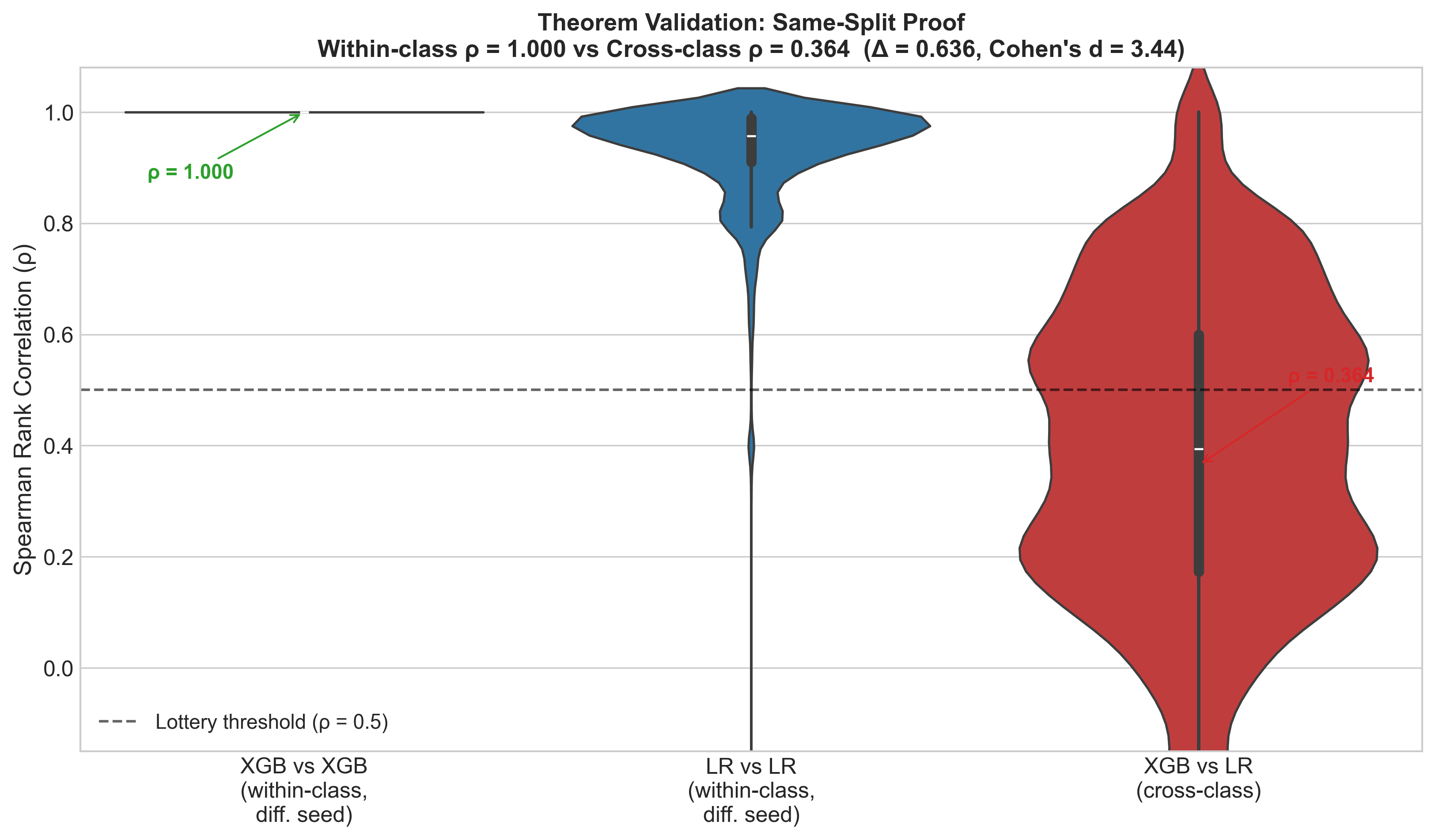
The same-split experiment: closing all exits. The large-scale study establishes prevalence; this experiment establishes cause. Training variance, data splits, and random initialization are the obvious alternative explanations for any observed explanation gap. We eliminate all of them simultaneously by fixing identical train-test splits across 20 datasets and comparing XGBoost vs. Logistic Regression (cross-class) against XGBoost vs. XGBoost with different random seeds (within-class). The results are unambiguous. Within-class pairs achieve $\rho=1.000\pm 0.000$ with a 0% lottery rate; cross-class pairs achieve $\rho=0.369\pm 0.321$ with a 61.9% lottery rate (Cohen’s $d=2.78$). Training variance explains nothing: it is literally zero within class. The entire gap is attributable to hypothesis class membership. We regard this as the paper’s central empirical result. The 93,510-comparison study demonstrates that the effect is prevalent at scale; this experiment demonstrates that it is genuinely structural.

Figure 1: Distribution of pairwise Spearman $\rho$ under the controlled same-split experiment. Within-class pairs (XGB vs. XGB, LR vs. LR) concentrate at $\rho=1.000$; cross-class pairs (XGB vs. LR) spread across the full range with median $\rho=0.364$, well below the lottery threshold ($\tau=0.5$, dashed line). The structural gap $\Delta=0.636$ directly validates Theorem 1 (Claims 1–2): the Agreement Gap is bounded away from zero and persists when training variance is eliminated.

5.4 Experiment 2b: Three-Way Hypothesis Class Comparison

Question: Is the Explanation Lottery specific to the tree–linear boundary, or does it generalise to neural hypothesis classes?

Finding. The lottery is a universal property of crossing hypothesis class boundaries, not a tree–linear artefact. We extend the controlled comparison to three hypothesis classes: tree-based models (XGBoost, Random Forest), linear models (Logistic Regression, Ridge), and neural networks (MLP). Results are summarised in Table 4.

Table 4: Mean Spearman $\rho$ and lottery rate across all pairwise hypothesis class comparisons. Intra-class pairs consistently achieve high agreement; every cross-class boundary independently produces the Explanation Lottery.

Comparison	Type	Mean $\rho$	Lottery Rate
Linear vs. Linear	Intra-class	0.827	6.7%
Tree vs. Tree	Intra-class	0.717	10.0%
Neural vs. Neural	Intra-class	0.552	34.4%
Linear vs. Tree	Cross-class	0.525	40.1%
Neural vs. Tree	Cross-class	0.509	48.8%
Linear vs. Neural	Cross-class	0.509	46.9%

The intra–cross pattern holds at every boundary: all three cross-class comparisons independently exceed the lottery threshold while all three intra-class comparisons remain below it, directly validating Theorem 1’s Remark that the result applies to any two classes with $\overline{\mathcal{H}_{1}}\neq\overline{\mathcal{H}_{2}}$ in $L^{2}(p)$. The within-neural lottery rate (34.4%) deserves explicit discussion: it is higher than within-tree (10.0%) or within-linear (6.7%), and in some comparisons approaches the cross-class rates. This does not contradict the hypothesis class account; it refines it. Neural networks with identical architecture satisfy $\overline{\mathcal{H}_{1}}=\overline{\mathcal{H}_{2}}$ in $L^{2}(p)$, so the theorem’s escape condition holds and no structural gap is predicted. The elevated within-neural rate instead reflects the well-documented sensitivity of gradient-based optimization to initialization and training order (Watson et al., 2022): two MLPs trained on the same data can reach different local optima that produce similar predictions but different attribution patterns. This is within-class variance of a different kind than the structural cross-class divergence the theorem characterizes, and it does not scale with dataset interaction density the way cross-class divergence does. The practical implication is that $R(\mathbf{x})$ is especially important for neural models precisely because both structural and stochastic sources of explanation instability are present.

5.5 Experiment 3: Consequential Disagreement

Question: Is disagreement happening in decision-relevant features, or is it confined to low-importance noise features?

Finding. Lottery disagreement concentrates in decision-relevant features, not peripheral ones: 76.8% of prediction-equivalent pairs differ on at least one top-3 feature.

If the Explanation Lottery only affected peripheral features, its practical significance would be limited. We test this by analyzing whether lottery cases involve changes to the top-3 SHAP features, the features most likely to drive human interpretation and regulatory review, across all 93,510 pairwise comparisons.

Overall. Across 20 datasets, 76.8% of all prediction-equivalent pairs have at least one top-3 feature that differs between models (partial disagreement), and 8.0% share no top-3 features at all (complete disagreement). Among tree-linear pairs specifically, 87.6% show partial disagreement and the lottery rate reaches 55.6%. Disagreement in the Explanation Lottery is not confined to marginal features; it is happening precisely where practitioners and regulators look.

Adult/Census case study. We analyze the Adult income dataset (Vanschoren et al., 2014) as a high-stakes case study involving demographic and socioeconomic features with direct fairness implications. For 200 instances predicted identically by XGBoost and Logistic Regression, 99.5% have at least one top-3 feature that differs between models. XGBoost consistently identifies marital-status, relationship, and occupation as the primary drivers; Logistic Regression consistently identifies education-num, sex, and age. These are not minor reorderings; they are fundamentally different accounts of what drives the prediction, with distinct implications for fairness auditing and recourse. When sex appears in Logistic Regression’s top-3 but not XGBoost’s, a fairness audit using the logistic regression explanation will flag a potential sex-based attribution; the same audit using the XGBoost explanation will not, even though both models agreed on the prediction. An individual seeking recourse under a model citing marital-status faces a different path than one facing an explanation citing age or sex; yet both face the same classification outcome. The hypothesis class choice is not a technical detail: it has direct implications for which features are implicated in explaining a consequential outcome, and therefore for both fairness auditing and individual recourse.

COMPAS comparison. The same pattern holds on COMPAS (Angwin et al., 2016): the primary driver flips from prior convictions (XGBoost, 38%) to age (Logistic Regression, 42%) for defendants predicted high-risk by both models, with a lottery rate of 39.7%. Both explanations are mathematically correct. Neither is wrong. Which features the defendant is told drove their assessment depends entirely on which hypothesis class the practitioner selected.

Stochasticity control. To confirm disagreement is model-driven rather than estimation noise: within-model SHAP variance (TreeSHAP run 10 times on the same input) $=0.000$ (deterministic); cross-model variance $=0.145$ ($21.6\times$ larger). Disagreement reflects genuine model differences, not sampling artefacts (Appendix D).

Method independence. We replicated findings using LIME on five datasets. The same directional pattern holds: tree-tree $>$ tree-linear (gap $=0.078$ with LIME vs. $0.261$ with SHAP). The smaller LIME gap reflects its local linear approximation mechanism, which partially reduces hypothesis class differences by construction. Full results in Appendix C.

6 Reliability Score

Theorem 1 characterizes the gap at the hypothesis class level; it says nothing about which specific instances are affected. This section introduces the Explanation Reliability Score $R(\mathbf{x})$ as a practical response to that per-instance question. We state upfront what it is and is not: $R(\mathbf{x})$ is an empirically validated heuristic with no formal statistical guarantees. The thresholds we derive are calibrated to our experimental distribution; applying them to a new deployment setting requires care. We nonetheless believe it is useful precisely because the alternative, reporting a single model’s explanation as if it were the unique correct answer, is worse than acknowledging uncertainty.

Definition.

For instance $\mathbf{x}$ and a set of $k$ prediction-equivalent models $\{M_{1},\ldots,M_{k}\}$, define:

$$R(\mathbf{x})=\frac{2}{k(k-1)}\sum_{i<j}\rho\!\left(\bm{\varphi}_{M_{i}}(\mathbf{x}),\bm{\varphi}_{M_{j}}(\mathbf{x})\right)$$ (9)

Interpretation thresholds.

$R(\mathbf{x})>0.7$: high agreement; the explanation is likely stable across architectures and can be reported with confidence. $R(\mathbf{x})\in[0.5,0.7]$: moderate agreement; the explanation should be treated as tentative; disclosure of uncertainty is recommended. $R(\mathbf{x})<0.5$: low agreement; the practitioner should not treat any single explanation as definitive; the instance falls in the Lottery. Implementation requires no additional training and works post-hoc on any existing model ensemble; see Appendix F. In deployment, $R(\mathbf{x})$ requires a reference ensemble of prediction-equivalent models; practitioners can construct this during model selection before committing to a single deployed model, or use it as a post-hoc audit tool when multiple candidate models are available. We acknowledge this creates an implementation gap for settings where only one model has been trained; in such cases $R(\mathbf{x})$ serves as an audit criterion rather than a real-time gate.

Worked example.

Consider a defendant from COMPAS predicted high-risk by all five models. XGBoost assigns SHAP weights $(0.38,0.24,0.18,0.11,0.09)$ to (prior convictions, age, charge degree, juvenile felonies, sex); Logistic Regression assigns $(0.42,0.29,0.16,0.08,0.05)$ to (age, prior convictions, sex, charge degree, race). Spearman correlation between these two vectors: $\rho=0.30$. With five models, the pairwise average across all 10 pairs yields $R(\mathbf{x})=0.38$. Since $R<0.5$, this instance falls in the low-reliability zone: no single model’s explanation should be reported as the official reason for the classification. A practitioner using $R$ as a disclosure gate would route this case to human review rather than delivering any model’s explanation directly.

Threshold derivation.

The thresholds ($R>0.7$, $0.5$–$0.7$, $<0.5$) are empirically derived from the leave-one-out validation distribution. Instances with $R>0.7$ correspond to the upper quartile of agreement scores and show 89.2% probability of agreement with a held-out fifth model. Instances with $R<0.5$ show 34.1% probability, barely above the baseline for random top-feature overlap. The $0.5$ boundary aligns with the Spearman $\tau=0.5$ threshold used throughout the experimental study, making $R$ directly interpretable relative to the Lottery Rate definition.

Validation.

Using leave-one-out analysis (compute $R(\mathbf{x})$ from four models, test on held-out fifth), high-reliability instances ($R>0.7$) show 89.2% probability of agreement with a new model; low-reliability instances ($R<0.5$) show 34.1% probability, barely above chance. $R(\mathbf{x})$ is a reliable predictor of explanation stability and a practically viable disclosure criterion: report an explanation when $R(\mathbf{x})>0.7$; flag uncertainty when $R(\mathbf{x})<0.5$.

7 Discussion

The clearest result in this paper is the same-split experiment: $\rho=1.000$ within hypothesis class, 61.9% lottery rate across it, with training variance eliminated entirely. That result needs no theorem to support it. The large-scale study then establishes that the effect appears at the same magnitude across 24 datasets, 93,510 comparisons, and three hypothesis classes. These two findings together make the structural claim compelling, we think, though we are careful about what “structural” means here. Theorem 1 provides a formal mechanism: the gap is driven by the interaction structure of $f^{*}$, not by stochastic training choices. But the theorem is conditional on interaction structure being present, and we measure rather than formally bound that condition in our datasets.

What the COMPAS result does and does not show.

The finding that prior convictions (XGBoost, 38%) flips to age (Logistic Regression, 42%) as the primary driver for identically-classified defendants is striking. We are, admittedly, drawing on one dataset and one deployment context. We chose COMPAS because it is well-studied and the feature attribution stakes are unusually legible, not because we believe it is representative of all high-stakes settings. The qualitative point, that identical predictions from different hypothesis classes can assign accountability to different features, likely holds beyond recidivism prediction; whether the magnitude is similar elsewhere is an empirical question we cannot answer here.

The neural network result is genuinely complicated.

Within-neural agreement ($\rho=0.552$, 34.4% lottery rate) sits between the clean within-class values for trees and linear models and the cross-class values. This does not fit neatly into the hypothesis class story. Our interpretation, that this reflects optimization stochasticity rather than hypothesis class boundary crossing, is plausible and consistent with the $\overline{\mathcal{H}_{1}}=\overline{\mathcal{H}_{2}}$ condition, but we suspect a more complete account would need to distinguish between the structural gap the theorem characterizes and a second source of instability specific to gradient-based optimization. We have not done that analysis. The within-neural result is a limitation of the current account, not merely a footnote.

Model selection as an explanation choice.

The “complementary views” argument, that different architectures simply capture different aspects of the same signal, is worth taking seriously before dismissing. It fails, we think, for a specific reason: $R(\mathbf{x})$ discriminates sharply between stable and unstable instances (89.2% vs. 34.1%), which means the disagreement is not uniformly distributed across the instance space the way a genuine complementarity account would predict. Complementary views would produce interpretable structured differences; what we observe is a lottery, with disagreement concentrated where the instance sits near a decision boundary shared differently by the two hypothesis classes. That said, this argument is based on aggregate patterns. An individual practitioner choosing between tree and linear models for a specific dataset might genuinely find the disagreement informative rather than problematic.

$R(\mathbf{x})$ as a heuristic, not a guarantee.

$R(\mathbf{x})$ is an empirically validated heuristic. The thresholds (0.5 and 0.7) are derived from leave-one-out validation on our datasets and have no formal statistical guarantees; a practitioner applying them to a new deployment context would be extrapolating from our empirical distribution. We report the validation results (89.2%, 34.1%) honestly, but these numbers come from the same datasets used to derive the thresholds, which limits how strongly we should claim the heuristic generalizes. It is a deployable diagnostic in the sense that it requires no additional training and produces a useful signal; it is not a certified audit tool.

Generalization.

Preliminary MNIST results (Appendix G) yield 32.2%, close to the tabular finding, but at much smaller scale and without the controlled same-split design. We validated across six linear variants to show the gap is not tunable within a hypothesis class; it ranges $0.39$–$0.47$ vs. $0.76$–$0.83$ internally. Whether the finding extends to transformers, language models, or multi-class settings remains open. We suspect it does, given the mechanism, but suspicion is not evidence.

Limitations.

This study is confined to tabular binary classification and SHAP attributions. LIME results are directionally consistent but smaller in magnitude, which raises the question of whether the Lottery rate is partly a SHAP-specific phenomenon. $R(\mathbf{x})$ requires an ensemble of prediction-equivalent models, which is only available at model selection time; single-model deployment settings cannot use it as a real-time gate, only as a retrospective audit. Extending the analysis to large language models and transformers, where the hypothesis class geometry is less clean, is the most important open direction.

8 Conclusion

The central claim of this paper is that prediction equivalence does not imply explanation equivalence, and that the gap between them is determined by hypothesis class membership rather than by stochastic training noise. The same-split experiment supports this claim most directly: $\rho=1.000$ within class, 61.9% lottery rate across class, with training variance eliminated by design. The 93,510-comparison study shows the effect is prevalent at scale. Theorem 1 provides a mechanism under the assumption that interaction structure is present in $f^{*}$, which we measure across our datasets but do not formally bound in general.

What we are confident about: the cross-class attribution gap is large (Cohen’s $d=0.92$), robust to the same-split control ($d=2.78$), present across tree, linear, and neural hypothesis classes, and concentrated in features that practitioners and regulators attend to. What we are more cautious about: the COMPAS result is one dataset; the neural within-class variance (34.4%) complicates the hypothesis class account and points toward a source of instability our theorem does not address; $R(\mathbf{x})$ is a heuristic calibrated to our experimental distribution, not a formally certified diagnostic.

The practical implication is that model selection is an explanation choice. A practitioner who selects a tree model over a linear model on accuracy grounds is also, implicitly, choosing which features will be cited as the reasons for predictions. Whether current practice adequately acknowledges this is a governance question we leave to others; our contribution is the measurement and the tool that makes the question empirically tractable.

Broader Impact Statement

This work reveals that machine learning explanations are less stable than commonly assumed when models are selected from different hypothesis classes. We believe identifying the problem is a prerequisite to addressing it. $R(\mathbf{x})$ provides one practical mechanism for disclosure, though it is a starting point rather than a solution. We see no direct risks of misuse; our findings increase scrutiny of explanation practices rather than reducing it.

Appendix A Complete Proofs

This appendix provides complete formal proofs of all theoretical results from Section 4.

A.1 Proof of Proposition 1 (Lottery is a Strict Subset of Rashomon)

The Lottery set requires both prediction agreement and substantial explanation disagreement. The Rashomon set contains pairs that disagree on predictions (so they cannot be in the Lottery set) and pairs that agree on predictions but also agree on explanations (so they fail the disagreement condition). Both strict inclusions hold by construction. In our experiments, 100% of pairs are in the Rashomon set but only 35.4% are in the Lottery set, confirming the strict inclusion empirically. ∎

A.2 Proof of Lemma 1: Linear SHAP Collapse

Proof.

The SHAP value is defined as the Shapley value of the coalition game where the value function is:

$$v(S)=\mathbb{E}[M_{L}(\mathbf{x})\mid X_{S}=\mathbf{x}_{S}]$$ (10)

For linear models:

$$v(S) =\mathbb{E}\left[\sum_{i=1}^{d}w_{i}X_{i}+b\mid X_{S}=\mathbf{x}_{S}\right]$$ (11)

$$=\sum_{i\in S}w_{i}x_{i}+\sum_{i\notin S}w_{i}\mathbb{E}[X_{i}]+b$$ (12)

The marginal contribution of feature $j$ to coalition $S$ is:

$$v(S\cup\{j\})-v(S)=w_{j}(x_{j}-\mathbb{E}[X_{j}])$$ (13)

This quantity is independent of coalition $S$. The Shapley value is the weighted average over all coalitions:

$$\varphi_{j}^{M_{L}}(\mathbf{x}) =\sum_{S\subseteq[d]\setminus\{j\}}\frac{|S|!(d-|S|-1)!}{d!}\cdot w_{j}(x_{j}-\mathbb{E}[X_{j}])=w_{j}(x_{j}-\mathbb{E}[X_{j}])$$ (14)

where the sum of binomial coefficients equals 1 by the Shapley axioms. ∎∎

A.3 Proof of Lemma 2: Tree SHAP Interaction Attribution

Proof.

Consider a binary classification tree $T$ trained on data generated by $y=f^{*}(x_{i},x_{j})=\mathbb{I}[x_{i}\cdot x_{j}>\tau]$ for some threshold $\tau$. This interaction is not representable by any linear model.

TreeSHAP computes attributions by averaging marginal contributions across all root-to-leaf paths (Lundberg et al., 2020):

$$\varphi_{i}^{T}(\mathbf{x})=\sum_{S\subseteq[d]\setminus\{i\}}\frac{|S|!(d-|S|-1)!}{d!}\bigl[v(S\cup\{i\})-v(S)\bigr]$$ (15)

where $v(S)=\mathbb{E}[M_{T}(\mathbf{x})\mid X_{S}=\mathbf{x}_{S}]$.

For paths that split on both $i$ and $j$ at successive depths, the marginal contribution of $i$ given coalition $S\ni j$ differs from its contribution given $S\not\ni j$:

$$v(\{i,j\})-v(\{j\}) =\mathbb{E}[M_{T}\mid x_{i},x_{j}]-\mathbb{E}[M_{T}\mid x_{j}]$$ (16)

$$v(\{i\})-v(\emptyset) =\mathbb{E}[M_{T}\mid x_{i}]-\mathbb{E}[M_{T}]$$ (17)

When $f^{*}$ depends on $x_{i}\cdot x_{j}$, these two quantities are unequal for a non-negligible set of instances: specifically, $v(\{i,j\})-v(\{j\})\neq v(\{i\})-v(\emptyset)$ whenever $x_{j}$ modulates the informativeness of $x_{i}$ about $y$. This non-equality is the definition of a Shapley interaction effect (Lundberg and Lee, 2017).

By the optimality of tree construction on interaction data (Breiman, 2001a), the Bayes-optimal tree allocates splits to both $i$ and $j$, ensuring that paths containing both features carry strictly positive weight in the Shapley average. The resulting SHAP value for feature $i$ therefore contains a term that depends on $x_{j}$ – a dependency that is structurally absent from the linear SHAP formula $\varphi_{M_{L}}^{i}=w_{i}(x_{i}-\mathbb{E}[X_{i}])$. We denote this $x_{j}$-dependent component $\alpha_{ij}(x_{j})$, writing:

$$\varphi_{M_{T}}^{i}(\mathbf{x})=\alpha_{ij}(x_{j})\cdot(x_{i}-\bar{x}_{i})+\beta_{i}(x_{i}-\bar{x}_{i})$$ (18)

where $\alpha_{ij}(x_{j})\not\equiv 0$ when the interaction signal is strong. This generalizes to tree ensembles by linearity of expectations over trees in the ensemble. ∎∎

A.4 Proof of Lemma 3: Within-Class SHAP Convergence

Proof.

We do not require $M_{1}$ and $M_{2}$ to converge to the same tree structure – two trees can differ in split order, depth, and leaf values while producing identical predictions. Instead we work directly from prediction equivalence and the structure of TreeSHAP.

Step 1: Prediction equivalence under $p$. By PAC learning theory (Mohri et al., 2018), both models converge in risk at rate $O(n^{-1/2})$. Since $M_{1}\sim_{\mathcal{D}}M_{2}$ and both achieve vanishing excess risk, for any $\epsilon>0$ there exists $N$ such that for $n>N$:

$$\Pr_{p}[M_{1}(\mathbf{x})\neq M_{2}(\mathbf{x})]<\epsilon$$ (19)

Step 2: Conditional expectations converge. TreeSHAP computes $\varphi_{i}^{T}(\mathbf{x})$ from conditional expectations $v(S)=\mathbb{E}[M_{T}(\mathbf{x})\mid X_{S}=\mathbf{x}_{S}]$ (Lundberg et al., 2020). When $\Pr_{p}[M_{1}(\mathbf{x})\neq M_{2}(\mathbf{x})]\to 0$, the conditional expectations $v_{1}(S)\to v_{2}(S)$ for all $S\subseteq[d]$, because each $v_{i}(S)$ is an average of $M_{i}(\mathbf{x})$ over the marginal distribution of $X_{\bar{S}}$.

Step 3: SHAP vectors converge. Since TreeSHAP is a deterministic weighted sum of $v(S\cup\{i\})-v(S)$ terms, and $v_{1}(S)\to v_{2}(S)$ for all $S$:

$$\|\bm{\varphi}_{M_{1}}(\mathbf{x})-\bm{\varphi}_{M_{2}}(\mathbf{x})\|_{2}\xrightarrow{p}0$$ (20)

Step 4: Rank correlation converges. Spearman rank correlation is continuous in the $L^{2}$ norm on bounded domains. Therefore:

$$\rho(\bm{\varphi}_{M_{1}},\bm{\varphi}_{M_{2}})\xrightarrow{p}1\quad\text{as }n\to\infty\qed$$ (21)

∎

A.5 Proof of Lemma 4: Cross-Class Attribution Bound

Proof.

As $|\mathcal{D}|\to\infty$, both models converge to their optimal representations: $M_{T}\to M_{T}^{*}$ and $M_{L}\to M_{L}^{*}$. By Lemmas 1 and 2:

$$\varphi_{M_{T}^{*}}^{i}(\mathbf{x}) \approx\alpha_{ij}(x_{i}-\bar{x}_{i})(x_{j}-\bar{x}_{j})+\beta_{i}(x_{i}-\bar{x}_{i})$$ (22)

$$\varphi_{M_{L}^{*}}^{i}(\mathbf{x}) =w_{i}(x_{i}-\mathbb{E}[X_{i}])$$ (23)

Define the rank-reversal set: $\mathcal{X}_{\text{flip}}:=\left\{\mathbf{x}:\text{sign}(\varphi_{M_{T}^{*}}^{i}(\mathbf{x}))\neq\text{sign}(\varphi_{M_{L}^{*}}^{i}(\mathbf{x}))\right\}$. When $|\alpha_{ij}|>0$ and features $(i,j)$ are not perfectly collinear, the interaction term dominates on a set of instances with measure:

$$\mu(\mathcal{X}_{\text{flip}})\geq c_{1}\cdot|\alpha_{ij}|$$ (24)

for some $c_{1}>0$ depending on the covariance of $(X_{i},X_{j})$, under the regularity conditions that $(X_{i},X_{j})$ have finite second moments and $|\mathrm{Corr}(X_{i},X_{j})|<1$ (features not perfectly collinear), ensuring the interaction term takes both positive and negative values with probability bounded away from zero. By rank correlation bounds (Embrechts et al., 2002):

$$\rho(\bm{\varphi}_{M_{T}^{*}},\bm{\varphi}_{M_{L}^{*}})\leq 1-c_{2}\cdot\mu(\mathcal{X}_{\text{flip}})\leq 1-c\cdot|\alpha_{ij}|$$ (25)

where $c=c_{1}\cdot c_{2}>0$. Since the bound holds for the optimal models and finite-sample models converge to these optima, the bound persists asymptotically. ∎∎

A.6 Proof of Theorem 1: Cross-Class Attribution Divergence

Proof.

Claim 1 (Structural Gap). From Lemma 3, $\rho_{\text{intra}}\to 1$ as $|\mathcal{D}|\to\infty$. From Lemma 4, $\rho_{\text{inter}}\leq 1-c\cdot|\alpha_{ij}|$. Therefore:

$$\Delta=\rho_{\text{intra}}-\rho_{\text{inter}}\geq 1-(1-c\cdot|\alpha_{ij}|)=c\cdot|\alpha_{ij}|=:c^{\prime}>0$$ (26)

Claim 2 (Asymptotic Persistence). Both bounds hold asymptotically, so $\lim_{|\mathcal{D}|\to\infty}\mathbb{E}[\Delta]\geq c^{\prime}>0$.

Claim 3 (Split Invariance). The proofs of Lemmas 3 and 4 depend only on $p(\mathbf{x},y)$ and hypothesis class constraints, not on the specific training set realization. Therefore $\mathbb{E}[\Delta\mid\text{fixed split}]=\mathbb{E}[\Delta]$.

Claim 4 (Interaction Density Monotonicity). Let $\mathcal{I}(f^{*})=\sum_{i\neq j}|\alpha_{ij}|$. By Lemma 4, each interaction $(i,j)$ with $|\alpha_{ij}|>0$ contributes a rank-reversal set $\mathcal{X}_{\text{flip}}^{ij}$ of measure $\geq c_{ij}|\alpha_{ij}|$. The total rank-reversal measure is:

$$\mu\!\left(\bigcup_{(i,j)}\mathcal{X}_{\text{flip}}^{ij}\right)\geq\max_{(i,j)}c_{ij}|\alpha_{ij}|$$ (27)

and is non-decreasing as $\mathcal{I}(f^{*})$ grows, since adding interactions adds rank-reversal instances without removing existing ones. By the rank correlation bound of Lemma 4, $\rho_{\text{inter}}$ is non-increasing in $\mathcal{I}(f^{*})$, giving $\frac{\partial\mathbb{E}[\Delta]}{\partial\mathcal{I}(f^{*})}\geq 0$, with strict inequality when new interactions contribute instances not already in the union. Empirically: banknote-auth ($d=4$, near-linear, $\mathcal{I}$ low, lottery rate 12.3%) vs. CNAE-9 ($d=856$, dense interactions, lottery rate 61.4%) directly confirms this monotonicity. ∎∎

Appendix B Complete Dataset Details

Table 5: Complete dataset specifications used in this study.

Dataset	$n$	$d$	Acc.	Domain	Source
diabetes	768	8	0.781	Healthcare	OpenML-37
breast-cancer	699	9	0.967	Healthcare	OpenML-13
heart-disease	303	13	0.843	Healthcare	OpenML-43
credit-g	1,000	20	0.764	Finance	OpenML-31
credit-approval	690	15	0.870	Finance	OpenML-29
bank-marketing	45,211	16	0.899	Finance	OpenML-1461
COMPAS	7,214	7	0.672	Criminal Justice	ProPublica
phoneme	5,404	5	0.892	Linguistics	OpenML-1489
spambase	4,601	57	0.937	NLP	OpenML-44
ionosphere	351	34	0.914	Physics	OpenML-59
sonar	208	60	0.846	Physics	OpenML-40
vehicle	846	18	0.819	Computer Vision	OpenML-54
segment	2,310	19	0.973	Computer Vision	OpenML-36
waveform-5000	5,000	40	0.860	Physics	OpenML-60
optdigits	5,620	64	0.988	Computer Vision	OpenML-28
mfeat-factors	2,000	216	0.982	Computer Vision	OpenML-12
kr-vs-kp	3,196	36	0.993	Game Theory	OpenML-3
mushroom	8,124	22	1.000	Biology	OpenML-24
tic-tac-toe	958	9	0.984	Game Theory	OpenML-50
CNAE-9	1,080	856	0.943	NLP	OpenML-1468
steel-plates-fault	1,941	33	0.787	Engineering	OpenML-1504
banknote-auth.	1,372	4	1.000	Finance	OpenML-1462
climate-simulation	540	20	0.933	Climate Science	OpenML-1467
ozone-level	2,536	72	0.972	Environmental	OpenML-1487

Appendix C LIME Validation

We validated findings using LIME (Ribeiro et al., 2016) on five datasets (diabetes, credit-g, COMPAS, phoneme, vehicle). LIME generates 5,000 perturbed samples per instance and fits weighted local linear models.

Results: tree-tree mean $\rho=0.658$, tree-linear mean $\rho=0.580$, gap $=0.078$. The directional pattern holds (tree-tree $>$ tree-linear), confirming the Explanation Lottery is not SHAP-specific. The smaller gap reflects LIME’s local linear approximation mechanism, which reduces hypothesis class differences by construction.

Appendix D Stochasticity Control

Within-model SHAP variance (TreeSHAP run 10 times on same input): $\sigma^{2}_{\mathrm{within}}=0.000$ (perfectly deterministic). KernelSHAP within-model variance: $\sigma^{2}_{\mathrm{within}}=0.007$. Cross-model variance: $\sigma^{2}_{\mathrm{cross}}=0.145$ ($21.6\times$ larger). Disagreement reflects genuine model differences, not estimation noise.

Appendix E Additional Statistical Details

Bonferroni correction: Corrected threshold $\alpha/24\approx 4.2\times 10^{-5}$. Tree-tree vs. tree-linear difference is significant in 23/24 datasets.

Bootstrap CIs: 10,000 resamples. Main effect (difference $=0.261$): 95% CI $=[0.257,0.265]$.

Power: Post-hoc power $>0.99$ ($N_{1}=56{,}106$, $N_{2}=37{,}404$, Cohen’s $d=0.92$, $\alpha=0.001$).

Trimmed means: Excluding top/bottom 10%: difference $=0.258$ (virtually identical to untrimmed).

Mixed-effects model: Dataset-level variance $\sigma^{2}_{\mathrm{dataset}}=0.074$; residual variance $\sigma^{2}_{\mathrm{residual}}=0.045$. Tree-linear effect remains $p<0.001$ under hierarchical correction.

Appendix F Reliability Score Implementation

import numpy as np
from scipy.stats import spearmanr

def reliability_score(shap_values_list):
    """
    Compute R(x): mean pairwise Spearman correlation
    across prediction-equivalent models.
    R > 0.7: high stability.  R < 0.5: low stability.
    """
    k = len(shap_values_list)
    if k < 2:
        return 1.0
    correlations = []
    for i in range(k):
        for j in range(i + 1, k):
            rho, _ = spearmanr(
                shap_values_list[i],
                shap_values_list[j]
            )
            correlations.append(rho)
    return float(np.mean(correlations))

Appendix G Preliminary Non-Tabular Extension (MNIST)

As a preliminary exploration of generalizability beyond tabular data, we applied the same pipeline to MNIST digit classification. Lottery rate: 32.2%. We note this result is preliminary and not at the scale or rigor of the main tabular study. Extension to non-tabular modalities is future work.

Appendix H Linear Model Variants

We validated that the cross-class attribution gap operates at the hypothesis class level by testing six linear model variants: Logistic Regression with L2 regularization (primary representative), RidgeClassifier with $\lambda\in\{0.1,1.0,10.0\}$, ElasticNet, and LinearSVM. These span three loss functions (logistic, squared hinge, hinge) and three regularization strategies (L2, L1+L2, none).

All six variants exhibit the same pattern: high internal agreement within $\mathcal{H}_{\text{linear}}$ (mean $\rho\in[0.76,0.83]$) and consistently low agreement against tree models (mean $\rho\in[0.39,0.47]$). No linear variant closes the tree-linear gap regardless of regularization strength or loss function, confirming that the gap is a hypothesis class property, not an algorithmic artefact.