Post-selected Criticality in Measurement-induced Phase Transitions

Abstract

Information-theoretic phase transitions, such as the measurement-induced phase transition (MIPT), characterize the robustness of quantum dynamics to local monitoring and are naturally formulated in terms of trajectories conditioned on typical measurement outcomes, which are naively accessible only through post-selection. Here we implement forced measurements to investigate how explicit post-selection alters the nature of the transition. We find that post-selection fundamentally alters the universality class by reweighting trajectories that are otherwise rare. In particular, we obtain a correlation-length exponent $\nu\approx 2.1$ larger than that of the standard MIPT and a negative effective central charge $c_{\mathrm{eff}}\approx-0.4$. We also compare the post-selected MIPT to the entanglement transition of Random Tensor Networks (RTN), and demonstrate that their universality class is the same. This setup further allows time-periodic, translationally-invariant circuits with post-selected weak measurements. In both models, we find that an onsite dimension of at least 3 (qutrits but not qubits) is necessary to induce a transition.

Introduction—Many-body quantum systems under unitary time evolution can be characterized by a growth of entanglement and scrambling of local information into non-local degrees of freedom when the dynamics is sufficiently ergodic. However, this growth can be slowed down and halted when local degrees of freedom are monitored, leading to a measurement-induced phase transition (MIPT) from an entangling phase to a disentangling phase [30, 22, 4, 5, 10, 2, 17, 23, 36, 11, 31, 32]. These information-theoretic phase transitions can be considered from various perspectives [10, 5, 3, 14]. A particularly insightful perspective is provided by starting from mixed states (rather than pure states) in the monitored circuit: in the area law phase, frequent measurements purify the state at a system-size independent rate, whereas in the volume law phase, the purification time diverges exponentially in the system size [10].

A similar entanglement transition was identified prior to the study of measurement-induced phase transitions in random tensor networks (RTNs), where the tensors are sampled from a distribution [33, 21, 12, 35]. In these networks, the boundary state undergoes an analogous area-to-volume law transition as one tunes the bulk bond dimension. While superficially unrelated, one can understand both the MIPT and the RTN transition through a mapping to a replica stat-mech model, where the transition manifests as an ordinary symmetry breaking transition in the effective “spin” degrees of freedom [33]. The crucial difference in their stat-mech description stems solely from the difference in sampling procedure: in MIPTs, measurement outcomes are sampled according to the Born distribution, whereas in RTNs the tensors are i.i.d. This stat-mech framework then leads to a rather non-trivial prediction: if one were to get rid of standard measurements that are governed by the Born rule and instead post-select to a fixed measurement outcome, the two transitions collapse to the same universality class.

Post-selection is already a heavily discussed topic in the literature on standard Born-rule MIPTs [9, 29, 34]. The purported “problem” stems from the fact that MIPTs are transitions of quantum trajectories and therefore can only be detected using quantities that are non-linear in the density matrix, in contrast to linear observables that can be characterized through the measurement-averaged density matrix. As a result, one must repeatedly sample the same quantum trajectory to observe the transition, an event that is exponentially rare in the extensive number of measurements, making experimental detection rather challenging. This issue has been partially mitigated for smaller system sizes using hybrid quantum circuits with cross-entropy benchmarking [26, 18, 13] and tomography techniques [19]. However, scaling to larger systems remains prohibitive due to the exponential growth of the Hilbert space, which necessitates either exponential computational resources for classical decoding or an exponential number of realizations of a quantum trajectory for reliable quantum state tomography.

Figure 1: (a-b): Schematic diagrams of both the models (a) Circuit diagram of the Random Quantum Circuit (RQC) (b) Circuit diagram of the Random Tensor Network (RTN) (c-f): Scaling collapse of various entanglement measures. Different system sizes are shown in shades of blue (Random Tensor Network) and red (Random Quantum Circuit). (c) Tripartite mutual information, $I_{3}$ near the critical point $p_{c}$. (d) Time evolution of the von Neumann entropy of an ancilla maximally entangled with $L$ qubits. (e) Von Neumann entropy of an ancilla entangled with a single qubit at $t>4L$ (f) Mutual information between ancillas entangled at sites $r$ and $r^{\prime}$ such that $|r-r^{\prime}|=L/2$.

Despite these difficulties, we now understand that MIPTs belong to a broader class of information-theoretic transitions, in which the two phases differ in how information spreads and whether it can be recovered from the system [5, 10, 3, 1, 6, 14]. From this perspective, a post-selected MIPT—where the model is defined ab initio by conditioning measurements on a fixed outcome—should no longer be viewed as pathological, but instead as a natural realization of a distinct universality class of such information-theoretic transitions, one that has received comparatively little attention in the literature (exceptions include monitored fermions, see Refs. [15, 16, 8, 28, 7]). The connection with RTNs makes the post-selected universality especially compelling since in RTNs the information-theoretic interpretation of the entanglement transition is natural: in the area-law phase, contracting the network is efficient, whereas in the volume-law phase it becomes exponentially hard in the system size.

In this letter, we numerically study both post-selected monitored quantum circuits and RTNs and characterize their critical properties. In particular, we report several critical exponents and confirm that the two models fall into the same “post-selected” universality class. To further probe the role of spatio-temporal randomness in these transitions, we reinstate spatial and time translational symmetries in both models in ways described in the main text. The evolution is then effectively implemented by a single transfer matrix. Interestingly, we observe a transition in the resulting RTN with three-state legs and in qutrit circuits, but not for qubits—raising the question of whether randomness within individual realizations is essential for the finite-$d$ monitored criticality.

principle

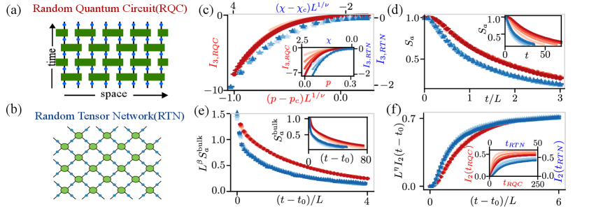
Models—The post-selected random quantum circuit (RQC) consists of two-qubit gates, $U_{i,i+1}$, drawn from the Haar distribution and arranged in a one-dimensional brick-layer geometry [37] with randomly interspersed forced measurements with probability $p$ that project the measured qubits onto $\ket{0}$. Fig. 1(a) depicts the gates as green rectangles and the forced measurements as blue circles. Numerically, we will consider systems of $L$ qubits with periodic boundary conditions and run the dynamics for a time $t\gtrsim 4L$ to reach a steady state unless otherwise specified. The rate of post-selected measurements $p$ is varied to probe the MIPT. Formally, a state $\ket{\psi_{t}}$ at a discrete time step $t$ is evolved via

$$\ket{\psi_{t+1}}=\prod_{i}M_{i}\prod_{i,\text{odd}}U_{i,i+1}\prod_{i}M_{i}\prod_{i,\text{even}}U_{i,i+1}\ket{\psi_{t}},$$

where $\ket{\psi_{t+1}}$ is the (unnormalized) state at time $t+1$, $M_{i}=P_{0}^{(i)}$ with (classical) probability $p$ and $M_{i}=I$ with probability $1-p$; $P_{0}^{(i)}$ is the projection onto the $\ket{0}$ state of qubit $i$, and $I$ is the identity operator. Note that the randomness in the model is entirely due to the random sampling of $M_{i}$ and $U_{i,i+1}$—there is thus no notion of quantum trajectories weighted by Born probabilities of different measurement outcomes.

An RTN is a two-dimensional network of local tensors $T_{\mu,\nu,\kappa,\lambda}$ (see Fig. 1b). The indices $\mu,\nu,\kappa,\lambda=1,\dots,D$ label states in the local qudit Hilbert space $\ket{1},\dots,\ket{D}$, where $D$ is the bond dimension of the network. The tensor entries are drawn independently from a Gaussian distribution with zero mean and unit variance. By adding a two-legged tensor (or equivalently, a quantum state) $\lambda_{\mu,\nu}$ on each edge $e$, we continuously tune the effective bond dimension of each leg by tracking the second Rényi mutual information, $\chi_{n=2}$, of the two-legged state $\ket{\lambda}=\sum_{\nu,\mu=1}^{D}\lambda_{\mu,\nu}\ket{\mu}\ket{\nu}$ across $e$. We will be interested in the state of the tensor network obtained at the boundary after the full contraction of the tensor network in the $L\times t$ lattice with periodic boundary conditions with the initial layer contracted at $t=1$ with a product initial state $\ket{0}^{\otimes L}$. We perform the contraction in a circuit-like fashion, as shown in Fig. 1b. Although this is not strictly necessary, it enables us to adapt well-established protocols for extracting critical data in MIPTs to the analogous setting of RTNs. Accordingly, throughout the rest of this work, we refer explicitly only to MIPT protocols, with the understanding that corresponding techniques apply analogously to RTNs. Calling the resulting contracted tensor $\mathcal{T}_{\mu_{1},\dots,\mu_{N}}$, the (unnormalized) wavefunction is $\ket{\psi}=\sum_{\mu_{1},\dots,\mu_{N}}\mathcal{T}_{\mu_{1},\dots,\mu_{N}}\ket{\mu_{1},\dots,\mu_{N}}$. Ref. [33] demonstrated that tuning the effective bond dimension $D_{\mathrm{eff}}$ drives an entanglement transition in the disorder averaged Rényi entanglement entropy of the normalized $\ket{\psi}$—from an area-law phase at small $D_{\mathrm{eff}}$ to a volume-law phase at large $D_{\mathrm{eff}}$. For a more detailed description, see the end matter.

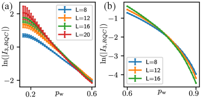
Results—At the entanglement transition, the entanglement behaves critically in the steady state of these models. To diagnose this, we first define the $n$th Rényi entropy $S_{n}(A)=\frac{1}{1-n}\ln\,\tr\rho_{A}^{n}$, where $\rho_{A}=\tr_{\bar{A}}\ket{\psi}\bra{\psi}$, and compute the tripartite mutual information ($I_{3,n}$) on four contiguous regions $A$, $B$, $C$, and $D$ of size $L/4$ [37]: For the von Neumann case, we write $I_{3}\equiv I_{3,1}$.

$$I_{3,n}(A,B,C)\equiv S_{n}(A)+S_{n}(B)+S_{n}(C)-S_{n}(A\cup B)\\ \quad-S_{n}(A\cup C)-S_{n}(B\cup C)+S_{n}(A\cup B\cup C).$$ (1)

We locate the critical point $p_{c}(\chi_{c})$ by identifying the measurement rate (bond-dimension) where the behavior of $I_{3,n}$ changes. In the area-law phase, $I_{3,n}$ approaches zero for large $L$ due to the cancellation of boundary contributions. In contrast, in the volume-law phase, $I_{3,n}$ exhibits a system-size dependence due to a non-zero bulk contribution [37], and at the critical point $I_{3,n}$ is scale invariant. From the exact numerical simulations of the RQC and the RTN, we use the scaling relation $I_{3,1}\sim f(L^{1/\nu}(p-p_{c}))$ to extract the critical points to be $p_{c,\mathrm{RQC}}=0.24(1)$ and $\chi_{c,\mathrm{RTN}}=0.9(9)$ and the correlation length exponents to be $\nu_{\mathrm{RQC}}=2.1(5)$ and $\nu_{\mathrm{RTN}}=2.2(5)$ for the two models. Since $\nu\gtrsim 2$, Harris’ criterion implies that the transition could be stable against static disorder [39]; an observation that would be interesting for future study.

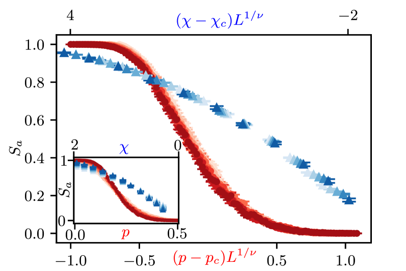
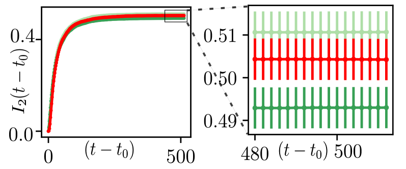
Coupling an ancilla locally with a system qubit by initializing them in a Bell state provides a local order parameter for purification [11, 10]. We obtain the density matrix of the ancilla $\rho_{a}$ by tracing out the system and we can compute $S_{a}=-\tr\rho_{a}\log\rho_{a}$ to diagnose purification. We consider this probe in three contexts. (1) We maximally entangle the ancilla with all qubits, then run the dynamics, tracking $S_{a}$ to diagnose purification. Using $S_{a}$, scaling yields $p_{c}=0.22(2)$ and $\chi_{c}=0.84(2)$ which agrees with the critical point obtained from $I_{3}$ (sxee End Matter for details). Applying the scaling form $S_{a}\sim g(t/L^{z})$ to the time evolution of $S_{a}$ at the critical point, we obtain the dynamical exponents $z_{\mathrm{RQC}}=0.96(5)$ and $z_{\mathrm{RTN}}=1.05(5)$ as shown in Fig. 1(d). (2) We run the full dynamics to a time $t_{0}>4L$ (steady-state) and couple in the ancilla locally in a Bell state to measure the local order parameter, $S_{a}^{\mathrm{bulk}}$. Using $S_{a}^{\mathrm{bulk}}$ and the scaling relation $S_{a}^{\mathrm{bulk}}\sim L^{-\beta}h\!\left((t-t_{0})/L^{z}\right)$, we extract the critical exponents $\beta_{\mathrm{RQC}}=0.16(5)$ and $\beta_{\mathrm{RTN}}\approx 0.16(2)$ as shown in Fig. 1(e). We also extracted the critical exponent of the Born-rule MIPT to be $\beta_{\mathrm{B-RQC}}=0.10(4)$. (3) We couple in two ancillas $a_{1}$ and $a_{2}$ into Bell states at either different locations or times and compute bipartite mutual information $I_{2}=S_{a_{1}}+S_{a_{2}}-S_{a_{1}a_{2}}$ to diagnose correlation functions. In this scenario, the ancillas are coupled in at a time $t_{0}>4L$ in the steady-state (bulk) and then evolved in time. Using $I_{2}$, we extract the spatial correlation exponent, finding $\eta_{\mathrm{RQC}}=0.17(2)$ and $\eta_{\mathrm{RTN}}=0.16(2)$, as shown in Fig. 1(f).

Model	$p_{c}$	$\nu$	$\eta$	$z$	$\beta$	$c_{\mathrm{eff}}$
P-RQC	$0.24(1)$	$2.1(4)$	$0.17(2)$	$0.96(5)$	$0.16(5)$	$-0.40(6)$
RTN	$0.9(9)$	$2.2(5)$	$0.16(2)$	$1.05(5)$	$0.16(2)$	$-0.35(2)$
B-RQC	$0.168(5)$	$1.2(2)$	$0.19(1)$	$1.06(4)$	$0.10(4)$	$0.25(3)$
P	$0.5$	$1.33$	$0.21$	$1$	$0.139$	$0.2914$

Table 1: Critical exponents for the phase transition in the post-selected random quantum circuit (P-RQC), the random tensor network (RTN), the Born-weighted random quantum circuit (B-RQC) [37, 36], and the percolation transition (P) [36].

Next, for both the post-selected MIPT and the RTN, the mapping to a statistical-mechanical model implicitly defines a partition function $Z_{X}=\tr[\rho_{X}]$, where $\rho_{X}=\ket{\psi_{X}}\bra{\psi_{X}}$ is the unnormalized pure-state density matrix obtained by evolving an initial state under a disorder realization $X$ to a final state $\ket{\psi_{X}}$ [20]. (Note that we use the term “disorder” here to denote random realizations of the circuits or tensors in the respective models, rather than quenched spatial randomness.) At sufficiently long times, any dependence on the initial state can be neglected. In the post-selected MIPT, $X$ specifies the measurement locations and gates, while in the RTN it specifies the realization of the random tensors. Equivalently, $Z_{X}$ is just the norm of the boundary state obtained after evolution with disorder realization $X$. As usual for disordered systems, one introduces the replica partition function $Z_{k}=\overline{[Z_{X}]^{k}}$ and the associated annealed free energy $F_{k}=-\log Z_{k}$, where the overbar denotes the disorder average over $X$. The quenched average free energy is then $F=\lim_{k\to 0}dF_{k}/dk=-\overline{\log[Z_{X}]}$, which is the quantity of interest for the post-selected MIPT and RTN.

For comparison, in Born-rule MIPTs one must also average over measurement trajectories $\mathbf{m}$ for a fixed $X$. The replica partition function then becomes $\tilde{Z}_{N}=\sum_{\mathbf{m}}p_{\mathbf{m}}Z_{\mathbf{m}}^{k}=\sum_{\mathbf{m}}Z_{\mathbf{m}}^{N}$, where $N=k+1$, $p_{\mathbf{m}}=Z_{\mathbf{m}}$, and where the average over disorder $X$ is now implicit. This extra replica changes the replica limit: the analogous free energy is $\tilde{F}=\lim_{N\to 1}d\tilde{F}_{N}/dN=-\sum_{\mathbf{m}}p_{\mathbf{m}}\log p_{\mathbf{m}}$, with $\tilde{F}_{N}=-\log\tilde{Z}_{N}$, so the limit is now $N\to 1$ rather than $0$. For fixed gates and measurement locations, this reduces to the Shannon entropy of the measurement record.

Now consider a system of size $L$ with periodic boundary conditions, evolved for $t\gg L$. The associated statistical-mechanical model lives on a cylinder of circumference $L$ and height $t$. Conformal invariance then fixes the finite-size scaling of the quenched free energy, more precisely its density, to take the form [24, 25]

Figure 2: (a) Schematic of the central charge $c(k)$ of the replica partition function $Z_{k}$. $k=0,1$ correspond to the post-selected and Born rule MIPTs respectively, and $k=2$ is the Ising model which has $c=1/2$.(b) Free-energy density $f(L)$ (see Eq. (2)) vs $1/L^{2}$.

$$\frac{F(L,t)}{A}=f(L)=f(L=\infty)-\frac{\pi c_{\mathrm{eff}}}{6L^{2}},$$ (2)

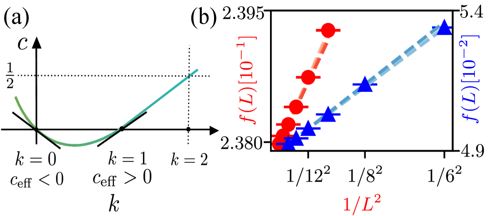
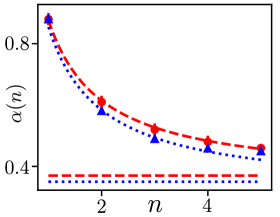
with the space-time area $A\equiv vLt$, where $v$ is the anisotropy factor calculated by comparing the temporal and spatial two-point correlation functions at the critical point [36] (see End Matter for details). Here $c_{\mathrm{eff}}$ is a universal number called the effective central charge, which is given by $c_{\mathrm{eff}}=\lim_{k\rightarrow 0}\left(dc(k)/dk\right)$, with $c(k)$ the central charge of the CFT describing the transition in the statistical model at a finite number of replicas with free energy $F_{k}=-\ln\overline{Z}_{k}$. The anisotropy factor for the RQC is computed to be $v_{\mathrm{RQC}}=0.70(6)$. As the RTN is symmetric under the exchange of space and time by construction, its anisotropy factor is $v_{\mathrm{RTN}}=1$. Fitting the free energy density, $F(L,t)/A=f(L)$, to the Casimir form in Eq. 2 yields the $c_{\mathrm{eff}}$ for the RQC and RTN models (See End Matter for details). We numerically estimate the effective central charges for the models to be $c_{\mathrm{eff,RQC}}=-0.40(6)$ and $c_{\mathrm{eff,RTN}}=-0.35(2)$. The negativity of $c_{\rm eff}$, although atypical, follows from three facts [27], namely, (i) $c(k)=0$ at both $k=0$ and $k=1$ due to trivial partition functions in these limits; (ii) for the Born-rule MIPT, the effective central charge at $k=1$, defined as $c_{\mathrm{eff}}(k=1)=\lim_{k\to 1}\frac{dc(k)}{dk}$ is positive [36]; and (iii) $c(k)$ is a continuous function of $k$ without additional zeroes. Together, (i)–(iii) imply that the slope of $c(k)$ at $k=0$ i.e., $c_{\mathrm{eff}}(k=0)=\lim_{k\to 0}\frac{dc(k)}{dk}$, must be negative as depicted in Fig. 2.

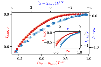
Translationally-invariant post-selected weak measurements— Post-selection, or equivalently removing randomness from the measurement trajectories, naturally prompts the question of what happens when all remaining randomness is eliminated, including that in the gates and measurement locations. The resulting evolution is governed by a single transfer matrix built from local non-unitary gates. One might naively expect this non-unitary evolution to mimic imaginary-time evolution toward the ground state of a local Hamiltonian with low entanglement, but it is unclear whether this intuition holds generically. To investigate this, we now turn to time-periodic, translationally-invariant systems where a single two-site unitary (or local tensor) is drawn once and repeated throughout the spacetime lattice. Interestingly, for the translationally-invariant RTN with three-state physical legs, we find an entanglement transition as we tune the effective bond dimension ($\chi$), captured by $I_{3}$ as shown in Fig. 3. The analogous fixed-unitary qubit circuit with post-selected weak measurements, however, shows no transition in $I_{3,1}$ (see End Matter for details)—but moving to qutrits restores the transition as the weak-measurement strength $p_{\mathrm{w}}$ is varied. This contrast suggests a strong dependence on the onsite Hilbert-space dimension; in particular, the qutrit transition indicates that randomness within individual realizations is not strictly necessary for MIPT criticality in these post-selected weak-measurement settings.

Figure 3: Tripartite mutual information $I_{3}$ for translationally-invariant post-selected weak-measurement variants.

Conclusion—We have characterized the universality of the post-selected MIPT and demonstrated its relation to the RTN model. The major differences in critical properties as compared to the standard MIPT (see Table 1) originate from a reweighting of trajectories (equivalently, the replica limit $k\to 0$). Furthermore, we find that the effective central charge is negative for this universality class which is rather unusual for disordered systems. Finally, we have also studied time-periodic, translationally-invariant variants with post-selected weak measurements, finding a transition in the translationally-invariant RTN with three-state legs and in qutrit circuits (see Fig. 3).

While the relationship is striking, there are still a few puzzles. For instance, in Fig. 1, the critical exponents are seen to match, but the scaling functions appear to differ. This suggests either that finite-size effects are not well captured at these system sizes or that there may be a more subtle difference between the two models that is not captured by the critical exponents. Furthermore, $\nu>2$ indicates that the system may be robust against static disorder, unlike the Born-rule MIPT which flows to infinite randomness [38]. Intriguingly, $p_{c}$ is larger after post-selection than it was in the Born-rule MIPT, suggesting that even naive selection of trajectories could enhance the volume-law phase’s ability to retain quantum information. We leave it to future work to explore whether this can be generalized or is a special feature of this model.

Appendix A Random Tensor Network (RTN)

To set notation, we briefly introduce the random tensor network (RTN) model [33] shown in Fig. 1(b). It is defined on a square lattice of size $L\times t$ with periodic boundary conditions, where each vertex-edge pair $(v,e)$ hosts a Hilbert space $\mathcal{H}_{ve}$ with basis states $\ket{\mu_{ve}}=\ket{1},\dots,\ket{D}$. Accordingly, one can associate to each bulk vertex $v$ the state

$$\ket{T_{v}}=\sum_{\mu_{ve_{1}},\dots,\mu_{ve_{z}}=1}^{D}T_{\mu_{ve_{1}},\dots,\mu_{ve_{z}}}\ket{\mu_{ve_{1}},\dots,\mu_{ve_{z}}},$$ (3)

where $z=4$ is the coordination number (see Fig. 1(b)), and $T_{\mu_{ve_{1}},\dots,\mu_{ve_{z}}}$ are the entries of the tensor at vertex $v$. These entries are sampled from a Gaussian distribution with zero mean, $\bar{T}_{\mu_{ve_{1}},\dots,\mu_{ve_{z}}}=0$, and unit variance, such that $\overline{T^{*}_{\mu_{ve_{1}},\dots,\mu_{ve_{z}}}T_{\nu_{ve_{1}},\dots,\nu_{ve_{z}}}}=\delta_{\mu_{ve_{1}},\nu_{ve_{1}}}\dots\delta_{\mu_{ve_{z}},\nu_{ve_{z}}}.$ At each edge, we define an entangled pair state

$$\ket{I_{e}}=\sum_{\mu_{ve},\mu_{v^{\prime}e}=1}^{D}\lambda_{ve,v^{\prime}e}\ket{\mu_{ve},\mu_{v^{\prime}e}},$$ (4)

where $(v,v^{\prime})$ are neighboring vertices connected by edge $e$. The matrix $\lambda$ controls the entanglement in $\ket{I_{e}}$ via the $n$-th Rényi mutual information

$$\chi^{(n)}_{e}=\frac{2}{1-n}\log\tr(\lambda\lambda^{{\dagger}})^{n},$$ (5)

which ranges from $0$ for a product state to $2\log D$ for a maximally entangled $D$-dimensional Bell state with $\lambda_{ve,v^{\prime}e}=D^{-1/2}\delta_{ve,v^{\prime}e}$. Thus, tuning $\lambda$ continuously interpolates the effective bond dimension between $0$ and $D$. For a given $\lambda$, we are interested in the properties of the state $\ket{\psi}$ obtained by contracting the tensor network:

$$\ket{\psi}=\bigotimes_{v}\bigotimes_{e}\bra{T_{v}}{I_{e}}\rangle,$$ (6)

where $\ket{\psi}$ resides on the physical legs at the top boundary of the network.

Appendix B Half-cut Entropy

To probe the entanglement structure of the system, we divide it into two equal partitions and compute the Rényi entropy of the subsystem. In the volume-law phase, $S_{n,1/2}\propto L$ (volume of the subsystem); in the area-law phase, $S_{n,1/2}\propto O(1)$(boundary of the subsystems); and at the critical point, $S_{n,1/2}\propto\alpha(n)\log L$.

Figure 4: Coefficients $\alpha(n)$ of the Renyi entropies (blue triangles: RTN; red circles: RQC). Blue dotted and red dashed lines show the $n$ dependence, and the horizontal lines denote $\alpha(\infty)$.

Model	$\alpha(1)$	$\alpha(2)$	$\alpha(3)$	$\alpha(4)$	$\alpha(5)$	$\alpha(\infty)$
P-RQC	$0.88(2)$	$0.61(2)$	$0.52(2)$	$0.48(2)$	$0.46(1)$	$0.37(2)$
RTN	$0.88(1)$	$0.581(2)$	$0.490(8)$	$0.459(7)$	$0.45(1)$	$0.35(1)$
B-RQC	$1.7(2)$	$1.2(2)$	—	—	$0.9(1)$	$0.7(1)$

Table 2: Critical exponents for the post-selected Random Quantum Circuit (P-RQC), the Random Tensor Network (RTN), and the Born-weighted Random Quantum Circuit (B-RQC) [37, 36].

The critical exponents $\alpha(n)$ for the Random Quantum Circuit and Random Tensor Network are consistent with each other and differ from the Born-rule MIPT, as shown in Table 2. For B-RQC, the dashes indicate values not explicitly tabulated in Refs. [37, 36]. Their $n$ dependence is $\alpha_{\mathrm{P-RQC}}(n)=0.53(3)/n+0.35(7)$ and $\alpha_{\mathrm{RTN}}(n)=0.55(2)/n+0.32(4)$, in contrast to $\alpha_{\mathrm{B-RQC}}(n)=1.0(1)/n+0.7(1)$.

Appendix C Purification transition

The measurement-induced phase transition can also be viewed as a purification transition. To probe this, we maximally entangle an ancilla with the system in a Bell state and compute its steady-state von Neumann entropy $S_{a}$ for different measurement rates, extracting $p_{c}$ and $\nu$ from the scaling collapse in Fig. 5.

Figure 5: Scaling collapse of the ancilla entropy $S_{a}$ near the critical point ($p_{c}$ for RQC, $\chi_{c}$ for RTN; red circles: RQC, blue triangles: RTN).

Appendix D Anisotropy Factor computation

The Random Quantum Circuit is anisotropic because the gates are unitary along the time axis but not along the spatial axis, unlike in a dual-unitary circuit where the anisotropy factor is 1.

Figure 6: Green curves show temporal correlations for qubits separated by $\Delta t=7L/16$ and $6L/16$ (dark to light); the red curve shows the spatial correlation for $\Delta r=L/2$.

Following the procedure used for the spatial correlation in the main text, the temporal correlation is obtained by entangling two ancilla qubits with the same qubit at times $(r,t)$ and $(r,t^{\prime})$. For $L=16$, the spatial correlation curve lies between the temporal curves for $t-t^{\prime}=6L/16$ and $7L/16$, giving $t^{*}\approx 6.36L/16$ by linear interpolation and hence $v=\ln(1+\sqrt{2})\frac{L}{\pi t^{*}}$.

Appendix E Effective Central Charge

The effective central charge of both the Random Quantum Circuit and the Random Tensor Network is obtained by fitting the finite-size scaling of the free energy $F$ (see main text) to the Casimir form in Eq. 2.

Figure 7: Free-energy density as a function of $1/L^{2}$ (red circles and dashed lines: RQC; blue triangles and dashed lines: RTN). Dashed lines give $m(L_{\mathrm{min}})$, and the inset shows the extrapolation to $m(\infty)$.

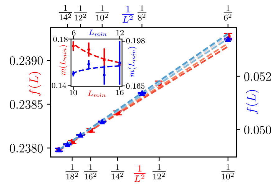
To reduce finite-size effects, we compute the slope $m(L_{\mathrm{min}})$ of $1/L^{2}$ using only system sizes $L>L_{\mathrm{min}}$. We then extrapolate $m(\infty)$ from $m(L_{\mathrm{min}})=m(\infty)+b/L_{\mathrm{min}}^{2}$, and compute $c_{\mathrm{eff}}=-6m(\infty)/\pi$.

Appendix F Translationally invariant circuit

As explained in the main text, we do not observe a MIPT for the translationally invariant RQC with qubits, but the transition reappears for qutrits. For qubits, the weak-measurement crossover $p_{\mathrm{w}}$ drifts to 0 with increasing system size; for qutrits it remains stable, consistent with a MIPT in the thermodynamic limit, as shown in Fig. 8.

Figure 8: $\ln|I_{3}|$ for the translationally invariant RQC: (a) qubits, (b) qutrits.