Deep Reinforcement Learning for Fano Hypersurfaces

Abstract.

We design a deep reinforcement learning algorithm to explore a high-dimensional integer lattice with sparse rewards, training a feedforward neural network as a dynamic search heuristic to steer exploration toward reward dense regions. We apply this to the discovery of Fano $4$-fold hypersurfaces with terminal singularities, objects of central importance in algebraic geometry. Fano varieties with terminal singularities are fundamental building blocks of algebraic varieties, and explicit examples serve as a vital testing ground for the development and generalisation of theory. Despite decades of effort, the combinatorial intractability of the underlying search space has left this classification severely incomplete. Our reinforcement learning approach yields thousands of previously unknown examples, hundreds of which we show are inaccessible to known search methods.

1. Introduction

We search a high-dimensional integer lattice directly inspired by the construction of Fano hypersurfaces, where each hypersurface is encoded as a lattice point. Our goal is to discover new Fano 4-fold hypersurfaces with terminal singularities, which correspond to the reward points in our search. The terminal condition gives rise to a reward landscape that is sparse and unknown a priori, yet spatially clustered, and it is this final attribute we will exploit. The search space is the $6$-dimensional integer lattice $\mathbb{Z}^{6}$, a $2$-dimensional projection of which is illustrated in Figure 1.

Figure 1. The $6$-dimensional dynamic heuristic (deep reinforcement learning) search for terminal Fano $4$-fold hypersurfaces projected onto $2$-dimensions. While the quasismooth terminal points are fully classified, the search discovers previously unknown nonquasismooth terminal ones. See Figure 9 for full details.

Exhaustive search algorithms have proven effective in low-dimensional cases, as is discussed in §3.1. In higher dimensions, however, the combinatorial explosion of the search space renders such methods infeasible for discovering examples with high degrees far from those already known. To overcome this, we introduce two algorithms. The first is a fixed heuristic search. The second, a dynamic heuristic search that builds upon the ideas of the first, in which we use a neural network as our heuristic and continuously update it via deep reinforcement learning. The fixed search is deterministic, whereas the dynamic search is nondeterministic due to a stochastic component that promotes exploration. The use of a compact neural network trained using temporal difference learning allows the dynamic heuristic to smooth over the high variance in the reward signal. The combination of this and the stochastic component allows regions of the search space to be reached that are computationally infeasible for the fixed heuristic to access. In our experiments, we found hundreds of examples lying in such regions.

This paper contributes to a growing body of work applying data science and machine learning to purely mathematical data, with early applications in algebraic geometry [1, 7, 8], subsequently expanding to other areas of mathematics [9, 10].

2. Integer Lattice Search

2.1. Setup

We begin by describing the setup of our search in the integer lattice $\mathbb{Z}^{n}$. The relation to searching for Fano $4$-fold hypersurfaces with terminal singularities is explained in §3.

Environment: An $n$-dimensional integer lattice, $\mathbb{Z}^{n}$, with a subset of points that we want to discover, that we will refer to as reward points.

Challenging properties:

1. Sparse: Reward points occupy a negligibly small fraction of the total search space.

2. Unknown a priori: Reward status of a point cannot be determined without direct evaluation.

Exploitable properties:

1. Spatially clustered: Reward points exhibit spatial locality, such that the presence of a reward point increases the likelihood of neighbouring points also being reward points.

Goal: To find both many and hard to reach reward points.

All attributes other than clustering pose challenges for constructing a search algorithm. Based on the clustering, we use previously found reward points in the search to inform where to search next. In both of the following algorithms, we construct heuristics that prioritise searching near denser regions of rewards.

2.2. Fixed Heuristic

The algorithm begins with a start point. We proceed by searching its neighbouring points and determining whether they are reward points. We add the neighbouring points to a search queue and assign them a priority value dependent on their proximity to previously found reward points. The function that computes this priority value is fixed, therefore making it a fixed heuristic algorithm. The algorithm resets by restarting the process with a point in the queue with the highest priority.

Figure 2. Flowchart of the fixed heuristic search algorithm.

The algorithm depicted in Figure 2 is performed as follows.

1. 1. Pick a start point $p\in\mathbb{Z}^{n}$, and set $v(p)=1$, where $v$ is the priority function defined in (3).

   2. Set the step count $s=0$ and fix the maximum step count $s_{\text{max}}\in\mathbb{N}$.

   3. Initialise the search queue $\mathcal{Q}$ as an empty heap.

2. Increment the step count $s$ by $1$. Identify all neighbouring points $\mathcal{N}$ of $p$, defined as the set of points exactly distance $1$ away under the $L^{1}$ norm, $\mathcal{N}:=\{n\in\mathbb{Z}^{n}\mid\|n-p\|_{1}=1\}$, in other words, all points differing by $\pm 1$ from $p$ in one coordinate.

3. For each $n\in\mathcal{N}$ determine its priority value

   $$v(n):=\begin{cases}1,&\text{if $n$ is a reward point,}\\ \tfrac{1}{2}v(p),&\text{otherwise},\end{cases}$$

   and add $(n,v(n))$ to the search queue $\mathcal{Q}$ if $n$ has never been added before.

4. Determine a point $p^{\prime}$ such that $(p^{\prime},v(p^{\prime}))\in\mathcal{Q}$ has the largest value $v(p^{\prime})$ in the heap. That is, take the first point of the heap ordered by priority values $v$. Set $p=p^{\prime}$ and remove $(p^{\prime},v(p^{\prime}))$ from $\mathcal{Q}$. Return to (2) if $s<s_{\text{max}}$, otherwise terminate the algorithm.

We observe in §3.3 that when the algorithm is applied to finding terminal Fano hypersurfaces, it is effective at finding many new examples in reward dense regions. We build on the ideas of the fixed heuristic search to design a dynamic heuristic search in §2.3 that can find reward points in lower density areas.

2.3. Dynamic Heuristic (Deep Reinforcement Learning)

The algorithm begins with a chosen start point. We compute its neighbours and, for each, determine the priority values assigned to them by a neural network function. We add these to a search queue ordered by priority values. Next, we assign rewards dependant on whether the neighbours added were reward points or not, and use these to update the neural network using temporal difference learning. The process is then repeated by searching a point with the highest priority in the search queue.

Figure 3. Flowchart of the dynamic heuristic search algorithm.

The algorithm depicted in Figure 3 is performed as follows.

1. 1. Pick a start point $p\in\mathbb{Z}^{n}$.

   2. Set the step count $s=0$, and fix the maximum step count $s_{\text{max}}\in\mathbb{N}$.

   3. Initialise a search queue $\mathcal{Q}$ as an empty heap.

   4. Create an MLP neural network $f_{\theta}\colon\mathbb{Z}^{n}\rightarrow\mathbb{R}$ with initial parameter $\theta$, this will be our dynamic heuristic that determines priority in the search queue $\mathcal{Q}$. Fix the temporal difference discount factor $\gamma\in(0,1)$, which affects how we update $f_{\theta}$ via temporal difference learning.

   5. Fix a standard deviation $\sigma\in\mathbb{R}_{\geq 0}$, this determines the stochastic component added to the priority value and thereby controls exploration.

   6. Fix $r_{\text{reward}}\in\mathbb{N}$, the value given for finding a reward point. Set $s_{\text{reward}}=0$, the number of steps since a reward was last found.

2. Increment the step count $s$ and steps since terminal $s_{\text{reward}}$ by $1$. Identify all neighbouring points $\mathcal{N}$ of $p$, defined as the set of points exactly distance $1$ away under the $L^{1}$ norm, $\mathcal{N}:=\{n\in\mathbb{Z}^{n}\mid\|n-p\|_{1}=1\}$, in other words, all points differing by $\pm 1$ from $p$ in one coordinate.

3. Determine whether any $n\in\mathcal{N}$ are reward points, and if so, reset $s_{\text{reward}}=0$. Compute their reward values

   $$r(n)=\begin{cases}r_{\text{reward}},&\text{if $n$ is a reward point},\\ -\sqrt{s_{\text{reward}}},&\text{otherwise}.\end{cases}$$

   Consider the set of tuples $(p,n,r(n))$ for each $n\in\mathcal{N}$. This data is used to train the network via temporal difference (TD) learning [19, §6]. To improve training stability, we fix a copy of the current network parameters, denoting them $\theta^{\prime}$, which remain frozen during this update step. For each $(p,n,r(n))$ for $n\in\mathcal{N}$, we compute their TD targets

   $$t(n)=r(n)+\gamma f_{\theta^{\prime}}(n),$$

   where $\gamma\in(0,1)$ is the discount factor controlling the trade off between short and long term rewards. Values of $\gamma$ close to $0$ produce greedy, short term behaviour whilst values close to $1$ encourage more long term behaviour. We then compute the TD error, measuring the discrepancy between the estimated value of $p$ and the TD target,

   $$\delta(\theta,p,n)=f_{\theta}(p)-t(n).$$

   Note that $\theta$ in $f_{\theta}(p)$ is updated during optimisation, whilst $t(n)$ is held fixed via $\theta^{\prime}$. Minimising $\delta(\theta,p,n)$ constitutes bootstrapping: future value estimates are refined using past ones. Concretely, we minimise the normalised mean squared error (MSE) loss

   $$L(\theta)=\tfrac{1}{2\lvert\mathcal{N}\rvert}\sum_{n\in\mathcal{N}}\delta(\theta,p,n)^{2},$$

   using a gradient based optimiser such as Adam.

4. For each $n\in\mathcal{N}$, compute their priority values $v(n)=f_{\theta}(n)+\varepsilon$, where $\varepsilon$ is sampled from $\mathcal{N}(0,\sigma^{2})$, a normal distribution with mean $0$ and variance $\sigma^{2}$. The stochastic component, $\varepsilon$, improves exploration. Add $(n,v(n))$ to the search queue $\mathcal{Q}$ if it has not previously been searched before.

5. Let $p^{\prime}$ be a point in the search queue $\mathcal{Q}$ such that $v(p^{\prime})$ is the largest value in the heap. That is, take the first point of the heap ordered by priority values $v$. Set the new search point $p=p^{\prime}$, and return to (2) if $s<s_{\text{max}}$, otherwise terminate the algorithm.

Since the dynamic heuristic search is nondeterministic, rerunning the algorithm can uncover new rewards within the same fixed number of steps. The search is also flexible in its objectives; the reward function can be modified to incentivise the discovery of points with specific properties, such as a high degree.

3. Fano 4-fold Hypersurfaces

3.1. Context

Algebraic varieties, the geometric shapes defined by polynomial equations, are central objects in mathematics. Among them, hypersurfaces, defined by a single polynomial equation, are the most tractable. A fundamental goal is to classify varieties into basic building blocks [18, §2.2]: Fano, Calabi-Yau, and general type with terminal singularities [17], a well known class of mild singularities. Birkar [2] proved that in any fixed dimension, only finitely many families of Fano varieties exist with terminal singularities, making a complete classification, in other words, building a ‘periodic table’, a finite problem. In dimensions 1, curves, and 2, surfaces periodic tables are known. In dimension 3, many important elements are known [4, 12, 13, 14]. Very little, however, is known in dimension $4$.

In dimension 3, Reid [11, §16.6 Table 5] produced a complete list of all $95$ Fano $3$-fold hypersurfaces with terminal singularities by a terminating algorithm [5, §2]. Iano-Fletcher [11, §16.7 Table 6] extended this to two equations, using a brute force search to find 85 families, working exhaustively from the origin of a search space of vectors $(a_{1},\ldots,a_{6})$ of integers $1\leq a_{1}\leq\ldots\leq a_{6}$, up to a fixed, arbitrary, limit of the degree $d=(\sum a_{i})-1=100$ where results seemed to have dried up. It was only much later that Chen, Chen and Chen [6] proved that Iano-Fletcher’s list is indeed complete. Such a search, run on hypersurfaces would take polynomial time $O(d^{4})$ in dimension $3$, and would recover Reid’s list of $95$. When moving to dimension $4$, it becomes $O(d^{5})$, and is no longer viable; the search space is too large, there are significantly more resulting cases, reward points have high degrees, and the complexity of determining terminality increases.

Figure 4. Exhaustive search of Fano 4-fold hypersurfaces with terminal singularities. In total $84,733$ terminal examples were found, $7,346$ quasismooth, and $77,387$ nonquasismooth. Each frame shows points in $\mathbb{Z}^{2}$, obtained by projecting the original $\mathbb{Z}^{6}$ search space onto consecutive coordinate pairs via $(a_{1},\ldots,a_{6})\mapsto(a_{i},a_{i+1})$.

When running the same exhaustive algorithm up to degree $d=200$ for Fano $4$-fold hypersurfaces with terminal singularities, we found $77,387$ new nonquasismooth examples, as illustrated in Figure 4. However, the search was unable to progress beyond this degree due to the polynomial increase in complexity at higher degrees. This computational bottleneck is precisely what both the fixed and dynamic heuristic algorithms of §2 are designed to overcome, by guiding the search rather than exhaustively exploring the space.

Figure 5. Classification of $11,617$ quasismooth Fano $4$-fold hypersurfaces with terminal singularities. Each frame shows points in $\mathbb{Z}^{2}$, obtained by projecting the original $\mathbb{Z}^{6}$ search space onto consecutive coordinate pairs via $(a_{1},\ldots,a_{6})\mapsto(a_{i},a_{i+1})$.

Brown and Kasprzyk [5] proved, however, that if one restricts to the far simpler subclass of quasismooth varieties, a complete classification in dimension 4 can be achieved. They found $11,617$ families of quasismooth Fano $4$-fold hypersurfaces; the list is on the Graded Ring Database [3]. Not only does quasismoothness make determining terminality easy and quick, using a cheap criterion, but it also provides a series of strong bounding conditions. This permits a terminating tree search algorithm that can be run in parallel, overcoming both the absence of a termination condition and the increase in complexity. Their classification establishes the assumption that nonquasismooth terminal points should also exhibit the same clustering behaviour exhibited by the quasismooth examples, as can be observed in Figure 5. This is further justified by the result in §3.2, which shows the criterion for determining terminality in the general setting, degenerates to the criterion in the quasismooth case.

Figure 6. The cumulative number of terminal Fano $4$-fold hypersurfaces found in the exhaustive search against degree.

In dimension 3, quasismoothness is well known to be an acceptable ‘generality’ assumption, which rules out few, if any, families. However, in dimension 4 the quasismooth assumption is far too strong: quasismooth Fano $4$-folds make up only a small fraction of all Fano $4$-fold hypersurfaces. Figure 6 depicts the cumulative number of quasismooth Fano $4$-fold hypersurfaces against nonquasismooth ones per hypersurface degree, illustrating the compelling reason why we must study the general case.

3.2. Background

To ground the general construction, we first illustrate it with a classical example, elliptic curves. The family of all elliptic curves is given by $X_{6}\subset\mathbb{P}(1,2,3)$. The ambient weighted projective space, $\mathbb{P}(1,2,3)=(\mathbb{C}^{3}\backslash\{0\})/\mathbb{C}^{*}$, where $\lambda\in\mathbb{C}^{*}$ acts on $\mathbb{C}^{3}\backslash\{0\}$ with coordinates $(x,y,z)$ via $\lambda\cdot(x,y,z)=(\lambda x,\lambda^{2}y,\lambda^{3}z)$. A curve in the family $X_{6}:(f_{6}=0)$ is the set of solutions of a homogeneous polynomial $f_{6}$ of degree $6$ which must be of the form

$$f_{6}=c_{1}z^{2}+c_{2}y^{3}+c_{3}x^{6}+c_{4}x^{4}y+c_{5}x^{2}y^{2}+c_{6}x^{3}z+c_{7}xyz$$

for some $c_{1},\ldots,c_{7}\in\mathbb{C}$, noting that $x$ has weight $1$, $y$ has weight $2$, and $z$ has weight $3$, so that each term does indeed have weight 6. Therefore, the family $X_{6}$ given by all possible equations $f_{6}$ is parametrised by its coefficients $[c_{1}:\cdots:c_{7}]\in\mathbb{P}^{6}$.

Extending the same construction to any weight $d$ and dimension $n$, we can define families of $n$-dimensional hypersurfaces

$$X_{d}\colon(f_{d}=0)\subset\mathbb{P}(a_{1},\ldots,a_{n+2})$$

for weights $1\leq a_{1}\leq\ldots\leq a_{n+2}$. As with the elliptic curve example, the family is parametrised by $\mathbb{P}^{N-1}$, where $N$ is the number of monomials of degree $d$ in weights $a_{1},\ldots,a_{n+2}$. We assume $X_{d}$ is well-formed [11, §6.10], in which case the adjunction number is defined as

$$\alpha=\sum^{n+2}_{i=1}a_{i}-d$$

and $X_{d}$ is Fano if $\alpha>0$, Calabi-Yau if $\alpha=0$, and general type if $\alpha<0$. For example, the elliptic curves $X_{6}\subset\mathbb{P}(1,2,3)$ have $\alpha=(1+2+3)-6=0$, and they are Calabi-Yau varieties. In the Fano case, we refer to the adjunction number as the Fano index $i_{X}=\alpha$. In this paper, we consider the main case of terminal Fano $4$-fold hypersurfaces, those of Fano index $i_{X}=1$. By fixing the Fano index, we have $d=\sum a_{i}-1$, and so may encode the data as an integer vector $(a_{1},\ldots,a_{6})\in\mathbb{Z}^{6}$ bounded by $1\leq a_{1}\leq\ldots\leq a_{n+2}$.

A

B

Figure 7. (7A) The real locus of the affine cone of the member of $X_{6}\subset\mathbb{P}(1,2,3)$ whose coefficients are all equal to $1$, which is quasismooth and hence admits only quotient singularities. (7B) The real locus of the affine cone of the member of $X_{10}\subset\mathbb{P}(1,3,4)$ whose coefficients are all equal to $1$, which is nonquasismooth; the hyperquotient singularity is visible as the line passing through the origin.

Next we come to the analysis of terminal singularities. On a hypersurface $X$, singularities can occur for two distinct reasons: either the derivative of the equation $f$ drops rank at a point $P\in X$, that is, all derivatives vanish at $P$, or the $\mathbb{C}^{*}$ quotient defining the ambient space has a nontrivial stabiliser at $P$. The latter case makes $P\in X$ a quotient singularity, and in this case we may use the computationally cheap criterion to determine terminality. By definition, quasismooth varieties have only such quotient singularities. Figure 7(7A) depicts such an example. In the former case, when the equation itself has a singularity, we refer to $P\in X$ as a hypersurface singularity. But, worse yet, our main concern is when both $P\in X$ is an equation singularity and the $\mathbb{C}^{*}$ quotient has a nontrivial stabiliser, we say $P\in X$ is a hyperquotient singularity, and think of it as composed of both the hypersurface equation singularity as a locus inside the ambient quotient space singularity. Such a singularity is visible in Figure 7(7B), where it is visible as the line passing through the origin.

We will search for general members of $X_{d}\subset\mathbb{P}(a_{0},\ldots,a_{n+2})$. Assuming generality means we study hypersurfaces corresponding to a dense open subset of the parameter space. This ensures that all members of the family share the same singularity structure, so we can compute a definitive list of singular points and analyse their terminality uniformly.

If $P$ is a quotient singularity [17, § 4], then it will be a singularity of type $\tfrac{1}{r}(b_{1},\ldots,b_{n})$ for some $r\geq 1$ and $b_{i}\geq 0$ such that $b_{i}\leq r-1$. The Reid–Shepherd-Barron–Tai criterion [16, §3.1][20, §3.2] says that $P$ is terminal if and only if

$$\tfrac{1}{r}\sum_{i=1}^{n}\overline{kb_{i}}-1>0,\quad\forall 1\leq k\leq r-1,$$

where $\overline{kb_{i}}\in\{0,\ldots,r-1\}$ denotes the residue of $kb_{i}$ modulo $r$.

If $P$ is a hyperquotient singularity [17, § 4], then it will be a singularity of type $\tfrac{1}{r}(b_{1},\ldots,b_{n+1};e)$ for some $r\geq 1$ and $b_{i}\geq 0$ such that $b_{i},e\leq r-1$. We approximate terminality by performing Mori’s criterion [15] restricted to the lattice points inside the unit cube. That is, we approximate $P$ to be terminal if either $r=1$, in which case it is a hypersurface singularity, or $r\geq 2$ and

$$\tfrac{1}{r}\sum_{i=1}^{n+1}\overline{kb_{i}}-\min\left\{\tfrac{1}{r}\sum^{n+1}_{i=1}m_{i}\cdot\overline{kb_{i}}\ \Bigg\lvert\ x_{1}^{m_{1}}\cdots x_{n+1}^{m_{n+1}}\in f^{\prime}\right\}-1>0,\quad\forall 1\leq k\leq r-1,$$

where $f^{\prime}$ is the local equation of $f$ on an affine patch that contains $P$. Notably, when $X_{d}$ is quasismooth, we will have $f^{\prime}=x_{i}+\cdots$ for some $1\leq i\leq n+1$, and therefore find that Mori’s criterion degenerates to the Reid–Shepherd-Barron–Tai criterion.

3.3. Analysis

We will apply both the fixed and dynamic heuristic algorithms of §2 to discover new Fano $4$-fold hypersurfaces with terminal singularities with Fano index $1$. The hypersurfaces are of the form $X_{d}\subset\mathbb{P}(a_{1},\ldots,a_{6})$, where $d=(\sum a_{i})-1$ and $1\leq a_{1}\leq\ldots\leq a_{6}$, and are encoded in our search as integer vectors $(a_{1},\ldots,a_{6})\in\mathbb{Z}^{6}$. Our goal is twofold: to identify as many new examples as possible and to uncover hard to reach ones. We show that the fixed heuristic search is particularly successful in the former, whilst the dynamic heuristic search achieves both.

To overcome the high degree obstruction faced by the exhaustive search as was discussed in §3.1, we will begin both the fixed and dynamic searches from the quasismooth terminal classification, which comprises $11,617$ cases. In practice, this means we force the first $11,617$ searched points in both algorithms to be the terminal quasismooth ones, and progress normally from then on. We run both the fixed and dynamic heuristic algorithms for $10,000,000$ steps. In the dynamic search, we use the hyperparameters in Table 1. Let $\mathcal{F}$ and $\mathcal{D}$ be the set of terminal points found by the fixed and dynamic searches, respectively. The fixed and dynamic searches are depicted in Figures 8 and 9 respectively.

Hyperparameter	Values
MLP Neural Network Layers	(40,)
Activation function	LeakyReLU
LeakyReLU slope	0.01
Optimiser	Adam
Optimiser learning rate	0.001
TD discount factor, $\gamma$	0.2
Standard deviation, $\sigma$	2
Search reward, $r_{\text{reward}}$	1

Table 1. Hyperparameters used in the dynamic heuristic (deep reinforcement learning) search.

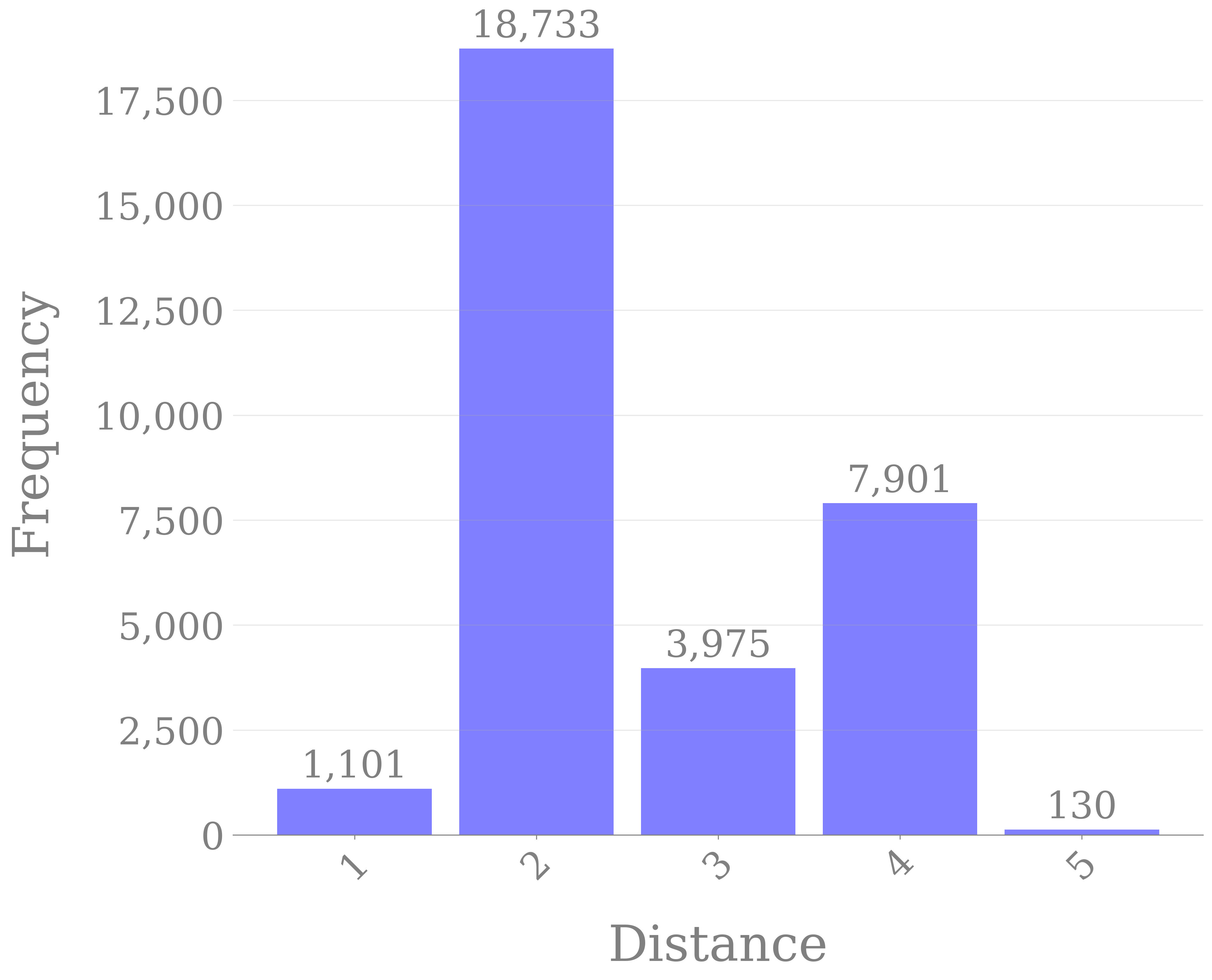
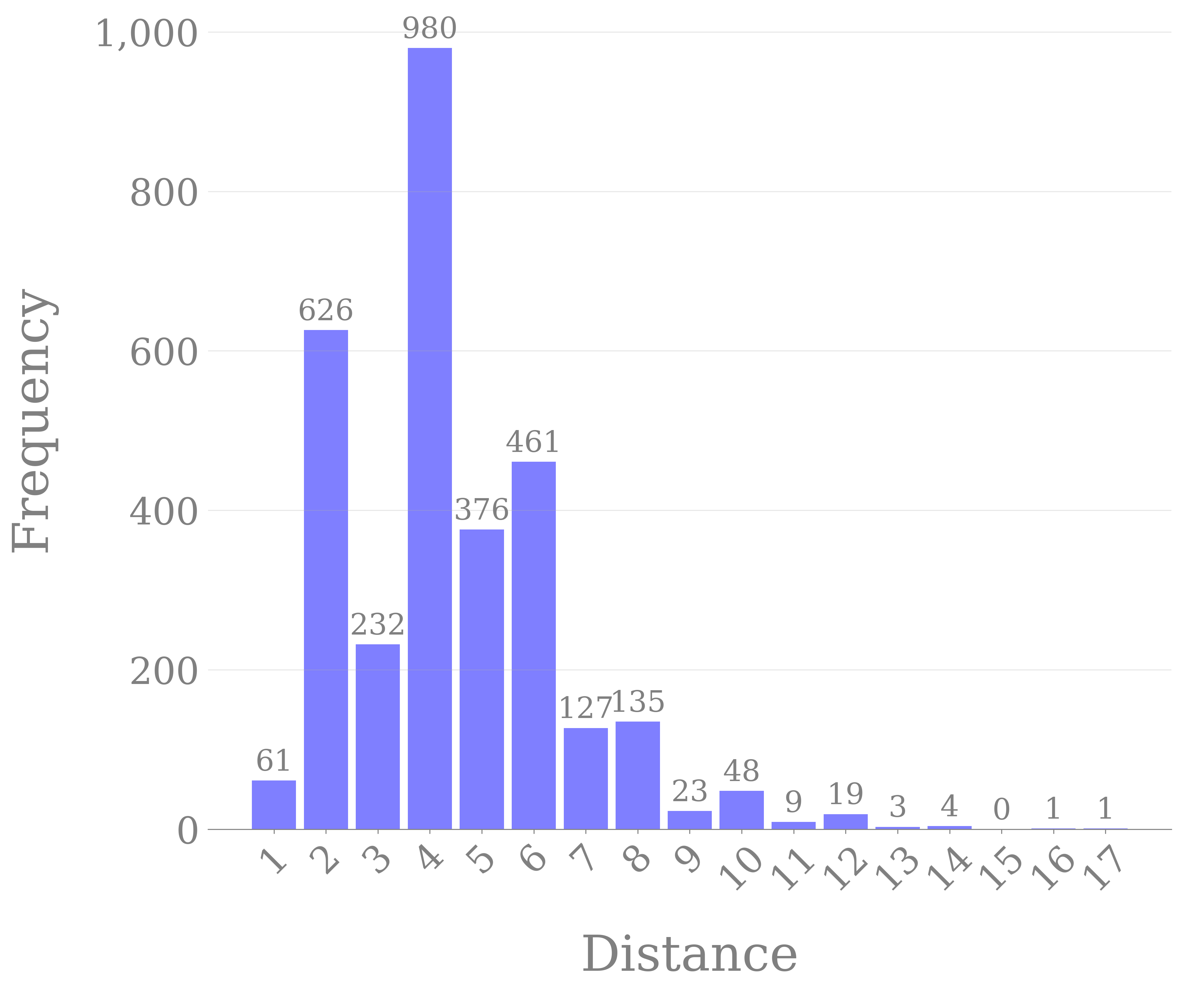
In the fixed heuristic search, we find $\lvert\mathcal{F}\rvert=113,996$ nonquasismooth Fano $4$-fold hypersurfaces with terminal singularities. The algorithm is deterministic, so it will discover the same examples on a rerun. It is particularly effective at finding a large quantity of new examples. It does, however, have limitations. As shown by the histogram in Figure 10(10A), the fixed search is unable to stray far from previously known reward points. The dynamic search found $\lvert\mathcal{D}\rvert=85,262$. Since the search is nondeterministic, each run will find a different set $\mathcal{D}$. Due to the more exploratory nature of the dynamic search, one expects fewer examples than the fixed one in the same step count, as a greater number of steps are spent in unprofitable regions during exploration. This is seen in Figure 10(10C). The histogram in Figure 10(10B) shows the upshot of this however. The figure shows hundreds of examples found by the dynamic search that are computationally inaccessible to the fixed one.

Figure 8. Fixed heuristic search. The search found $113,996$ nonquasismooth Fano $4$-fold hypersurfaces with terminal singularities. Each frame shows points in $\mathbb{Z}^{2}$, obtained by projecting the original $\mathbb{Z}^{6}$ search space onto consecutive coordinate pairs via $(a_{1},\ldots,a_{6})\mapsto(a_{i},a_{i+1})$.

Figure 9. Dynamic heuristic (deep reinforcement learning) search. The search found $85,262$ nonquasismooth Fano $4$-fold hypersurfaces with terminal singularities. Each frame shows points in $\mathbb{Z}^{2}$, obtained by projecting the original $\mathbb{Z}^{6}$ search space onto consecutive coordinate pairs via $(a_{1},\ldots,a_{6})\mapsto(a_{i},a_{i+1})$.

To measure the inaccessibility of points found exclusively by the dynamic search, we analyse two sets: $\mathcal{F}\backslash\mathcal{D}$, the $31,480$ points found by the fixed but not the dynamic search, and $\mathcal{D}\backslash\mathcal{F}$, the $3,106$ points found by the dynamic but not the fixed search. For each point in $\mathcal{F}\backslash\mathcal{D}$, we compute the shortest distance under the $L^{1}$ norm to the nearest point in $\mathcal{D}$. For each point in $\mathcal{D}\backslash\mathcal{F}$, we compute the shortest distance to the nearest point in $\mathcal{F}$. From these distances we derive a lower bound on the number of steps required to reach a point from its nearest neighbour. This allows us to show that hundreds of points found by the dynamic search would be computationally expensive to find using the fixed search alone. Combined with the fact that the search was initialised from $11,617$ starting points, this demonstrates that such points are effectively computationally inaccessible to the fixed search.

Explicitly, for a point $p\in\mathcal{F}\backslash\mathcal{D}$ (resp. $\mathcal{D}\backslash\mathcal{F}$), we define the shortest distance

$$D(p):=\min\{\|p-q\|_{1}\mid q\in\mathcal{F}\backslash\{p\}\text{ (resp. $\mathcal{D}\backslash\{p\}$)}\}.$$

Let $q$ denote the nearest neighbour of $p$, so that $\|p-q\|_{1}=D(p)$. We now derive lower and upper bounds on the number of steps required to find $p$ starting from $q$. We first assume that $p$ is the closest point to $q$ in the relevant set. Relaxing this assumption leaves the lower bound unchanged, it only weakens it, but invalidates the upper bound, since the search may be steered away from $p$ by a closer point. Alternatively, replacing the priority function in the fixed search with the constant function $v(n):=1$ ensures both bounds remain valid. The fixed search exhaustively expands points in order of increasing $L^{1}$ distance from $q$, visiting all points at distance $1$, then $2$, and so on. Consequently, to reach a point at distance $D(p)$, the search must first visit at least one point at distance $D(p)-1$, and must have already visited all points at distance $\leq D(p)-2$. This gives a lower bound on the number of steps for $p$ to be found from $q$,

$$s_{L}(p)=\#\{(a_{1},\ldots,a_{6})\in B(q,D(p)-2)\cap(\mathbb{Z}^{6}\cap(a_{1}\geq 1)\bigcap_{i=1}^{5}(a_{i}\leq a_{i+1}))\}+1.$$

Assuming either $p$ is the closest point to $q$, or using $v(n):=1$ as the priority value, we must have found $p$ after searching all points of distance $D(p)-1$, and so obtain an upper bound

$$s_{U}(p)=\#\{(a_{1},\ldots,a_{6})\in B(q,D(p)-1)\cap(\mathbb{Z}^{6}\cap(a_{1}\geq 1)\bigcap_{i=1}^{5}(a_{i}\leq a_{i+1}))\}.$$

Moreover, the likelihood that the lower bound becomes weaker grows with $D(p)$. We establish both bounds under the assumption that $p$ is the closest point to $q$; under this assumption, $p$ is guaranteed to be found within $s_{U}(p)$ steps, which, as noted above, would be even larger without this assumption. The probability of finding $p$ in $s_{L}(p)\leq s\leq s_{U}(p)$ many steps is then given by

$$P(s)=\frac{s-(s_{L}(p)-1)}{s_{U}(p)-(s_{L}(p)-1)}$$

as it must be found by a point of distance $D(p)-1$, of which there are $s_{U}(p)-(s_{L}(p)-1)$. Therefore, the probability of the lower bound being achieved is $1/(s_{U}(p)-(s_{L}(p)-1))$, which increases with $D(p)$.

Almost all examples have weight $a_{1}=1$, weakening the lower bound. The reduction of the bound caused by cases where $a_{i}-D(p)<1$ for $i\geq 2$, and $a_{i+1}-a_{i}-D(p)<0$ for $i\geq 1$, were in practice found to be negligible. Overlooking this allows us to give an approximation for the lower bound. Assuming $a_{1}=1$, $a_{i}-D(P)\geq 1$, $a_{i+1}-a_{i}-D(p)>0$,

$$s_{L}(p)=\#\{(a_{1},\ldots,a_{6})\in B(0,D(p)-2)\cap(\mathbb{Z}^{6}\cap(a_{1}\geq 0))\}+1.$$

Using this, when $D(p)=5$, we obtain $s_{L}(p)=305$, whereas, for $D(p)=15$ we get $227,305$, for $D(p)=16$ it is $528,865$ and for $D(p)=17$ it is $774,912$. To put the expense of these large $D(p)$ points into perspective, one should note that executing the full $10,000,000$ step fixed search was itself costly.

A

B

C

Figure 10. (10A) A histogram showing the distribution of distances from points found in the fixed but not dynamic search to their closest neighbours. (10B) A histogram showing the distribution of distances from points found in the dynamic but not fixed search to their closest neighbours. The dynamic search finds points at greater distances than the fixed search, corresponding to points that are increasingly inaccessible to the latter. (10C) A graph showing the number of nonquasismooth terminal examples found against the number of steps taken by the search. As expected, the dynamic search finds fewer terminal points in the same number of steps as the fixed one, since more steps are spent in unprofitable territory in order to reach terminal points at greater distances.

Consider $X_{1020}\subset\mathbb{P}(1,15,32,139,340,494)$, a point found in the dynamic but not the fixed search. Its closest point is $X_{1011}\subset\mathbb{P}(1,10,31,143,337,490)$, a quasismooth start point, at distance $17$. Our approximation predicts at least $774,912$ steps are required to reach it. By setting $v(n):=1$ in the fixed search we located it in $1,041,501$ steps. However, using the original priority value, the search is directed away from $X_{1020}$, and even after $10,000,000$ steps starting from $X_{1011}$ alone, it remains out of reach.

As Figure 10(10B) illustrates, among all points found by the dynamic search but not the fixed one, hundreds lie far from any other point, and are therefore beyond the computational reach of the fixed search.

Code and Data Availability

All code required to replicate the results is available on GitHub [21] under an MIT license, along with all datasets.

References

- [1] (2024) New Calabi-Yau manifolds from genetic algorithms. Phys. Lett. B 850, pp. Paper No. 138504, 10. External Links: ISSN 0370-2693,1873-2445, Document, Link, MathReview (Gleb A. Koshevoy) Cited by: §1.
- [2] (2021) Singularities of linear systems and boundedness of Fano varieties. Ann. of Math. (2) 193 (2), pp. 347–405. External Links: ISSN 0003-486X,1939-8980, Document, MathReview (James McKernan) Cited by: §3.1.
- [3] (2007-present) The graded ring database. Note: https://grdb.co.uk Cited by: §3.1.
- [4] (2022) Kawamata bounds for Fano threefolds and the Graded Ring Database. (), pp. 23pp. Note: arXiv:2201.07178 Cited by: §3.1.
- [5] (2016) Four-dimensional projective orbifold hypersurfaces. Exp. Math. 25 (2), pp. 176–193. External Links: ISSN 1058-6458,1944-950X, Document, Link, MathReview (Howard Nuer) Cited by: §3.1, §3.1.
- [6] (2011) On quasismooth weighted complete intersections. J. Algebraic Geom. 20 (2), pp. 239–262. External Links: ISSN 1056-3911,1534-7486 Cited by: §3.1.
- [7] (2023) Machine learning detects terminal singularities. In Advances in Neural Information Processing Systems, A. Oh, T. Naumann, A. Globerson, K. Saenko, M. Hardt, and S. Levine (Eds.), Vol. 36, pp. 67183–67194. Cited by: §1.
- [8] (2023) Machine learning the dimension of a Fano variety. Nature Communications 14 (1), pp. 5526. External Links: Document, Link, ISSN 2041-1723 Cited by: §1.
- [9] (2021) Advancing mathematics by guiding human intuition with AI. Nature 600 (7887), pp. 70–74. External Links: Document, Link, ISSN 1476-4687 Cited by: §1.
- [10] (2024) AI-driven research in pure mathematics and theoretical physics. Nature Reviews Physics 6 (9), pp. 546–553. External Links: Document, Link, ISSN 2522-5820 Cited by: §1.
- [11] (2000) Working with weighted complete intersections. In Explicit birational geometry of 3-folds, London Math. Soc. Lecture Note Ser., Vol. 281, pp. 101–173. External Links: MathReview (Roberto Muñoz) Cited by: §3.1, §3.2.
- [12] (1977) Fano threefolds. I. Izv. Akad. Nauk SSSR Ser. Mat. (no. 3,), pp. 516–562, 717. External Links: ISSN 0373-2436, MathReview (Miles Reid) Cited by: §3.1.
- [13] (1978) Fano threefolds. II. Izv. Akad. Nauk SSSR Ser. Mat. (no. 3,), pp. 506–549. External Links: ISSN 0373-2436, MathReview (Miles Reid) Cited by: §3.1.
- [14] (1983) On Fano -folds with . In Algebraic varieties and analytic varieties (Tokyo, 1981), Adv. Stud. Pure Math., Vol. 1, pp. 101–129. External Links: ISBN 0-444-86612-4, Document, MathReview (I. Dolgachev) Cited by: §3.1.
- [15] (1985) On -dimensional terminal singularities. Nagoya Math. J. 98, pp. 43–66. External Links: ISSN 0027-7630,2152-6842, Document, Link, MathReview (David R. Morrison) Cited by: §3.2.
- [16] (1980) Canonical -folds. In Journées de Géometrie Algébrique d’Angers, Juillet 1979/Algebraic Geometry, Angers, 1979, pp. 273–310. External Links: ISBN 90-286-0500-2, MathReview (Jayant M. Shah) Cited by: §3.2.
- [17] (1987) Young person’s guide to canonical singularities. In Algebraic geometry, Bowdoin, 1985 (Brunswick, Maine, 1985), Proc. Sympos. Pure Math., Vol. 46, Part 1, pp. 345–414. External Links: ISBN 0-8218-1476-1, Document, Link, MathReview (Eckart Viehweg) Cited by: §3.1, §3.2, §3.2.
- [18] (2002) Update on 3-folds. In Proceedings of the International Congress of Mathematicians, Vol. II (Beijing, 2002), pp. 513–524. External Links: ISBN 7-04-008690-5, MathReview (A. S. Tikhomirov) Cited by: §3.1.
- [19] (2018) Reinforcement learning: an introduction. 2nd edition, MIT Press, Cambridge, MA. External Links: ISBN 9780262039246 Cited by: item 3.
- [20] (1982) On the Kodaira dimension of the moduli space of abelian varieties. Invent. Math. 68 (3), pp. 425–439. External Links: ISSN 0020-9910,1432-1297, Document, Link, MathReview (K.-B. Gundlach) Cited by: §3.2.