Abstract

Mathematical models of biological populations commonly use discrete structure classes to capture trait variation among individuals (e.g. age, size, phenotype, intracellular state). Upscaling these discrete models into continuum descriptions can improve analytical tractability and scalability of numerical solutions. Common upscaling approaches based solely on Taylor expansions may, however, introduce ambiguities in truncation order, uniform validity and boundary conditions. To address this, here we introduce a discrete multiscale framework to systematically derive continuum approximations of structured population models. Using the method of multiple scales and matched asymptotic expansions applied to discrete systems, we identify regions of structure space for which a continuum representation is appropriate and derive the corresponding partial differential equations. The leading-order dynamics are given by a nonlinear advection equation in the bulk domain and advection-diffusion processes in small inner layers about the leading wavefronts and stagnation point. We further derive discrete boundary layer descriptions for regions where a continuum representation is fundamentally inappropriate. Finally, we demonstrate the method on a simple lipid-structured model for early atherosclerosis and verify consistency between the discrete and continuum descriptions. The multiscale framework we present can be applied to other heterogeneous systems with discrete structure in order to obtain appropriate upscaled dynamics with asymptotically consistent boundary conditions.

1 Introduction

Biological organisation is commonly underpinned by structure, which refers to organised heterogeneity, from the population-level (e.g. age, size) to phenotypic differences within cellular environments. This heterogeneity shapes individual interactions, development, and population dynamics. Structured mathematical models provide a framework for representing biological heterogeneity by introducing internal state variables into the population description, often using a discrete framework to capture distinct states or groups (36, 43). Such models are used in various fields, including epidemiology (age-based disease transmission analysis) (40, 16, 34), cell biology (cell cycle transitions, phenotype switching, exhaustion, migration) (42, 13, 23, 12), atherosclerosis (lipid metabolism and accumulation, and macrophage behaviour) (11, 14, 6, 7, 8), and agent-based models, e.g. (9, 38, 21, 44, 37, 12, 30).

Mathematically, structured heterogeneity in discrete frameworks is often represented by a large system of coupled equations, which can be challenging to analyse directly. Continuum approximations typically recast the dynamics in terms of partial differential equations (PDEs), which can be more amenable to investigation by a wider range of analytical techniques. Additionally, while a discrete system must scale with the number of discrete structured classes, describing this limit via a smooth field using a PDE description allows for more scalable numerical solutions. Discrete-to-continuum approaches which retain the essential features of the original system are therefore a central tool in structured models (3), but as we shall see there is considerable nuance in how continuum limits should be taken (43).

A standard method for obtaining continuum approximations involves using a Taylor series expansion (see e.g. (6, 9, 37, 15, 28, 2, 20, 22)). The discrete population is represented by a continuous density in the limit of many structure classes and a Taylor series expansion is applied to the discrete system. Truncating this expansion at a specific order yields a PDE that approximates the original model. However, the resulting PDEs may not be uniformly valid across the entire domain, especially in the presence of boundary layers or degenerate regions, where rapidly varying dynamics occur. Moreover, the appropriate order of truncation can be unclear since different choices can lead to inconsistent results across models (23, 9). Additionally, the number and form of the boundary conditions used to close the PDE depend on the chosen truncation order, and it is not always clear what boundary conditions are appropriate to impose in the continuum model. Similar difficulties arise in agent-based models (9, 38, 21, 44), where coarse graining (37, 12) and mean-field approximations (30) are often used to derive continuum approximations. These unresolved issues demonstrate the need for alternative, more formal approaches to continuum approximations.

The method of multiple scales applied to discrete systems provides a systematic alternative to Taylor expansions for deriving continuum approximations. It analyses difference equations by introducing a discrete short scale and a continuum long scale and uses matched asymptotic expansions to construct uniformly valid approximations. First introduced to study discrete difference equations (18), it has since been applied to linear and nonlinear difference equations (24, 25, 33, 41, 27), the discrete Painlevé equation (19), nonlinear wave propagation (26), first integrals for difference equations (32), functional equations (31), and the discrete logistic equation (17). In mathematical biology, it has been used to derive continuum descriptions of Delta–Notch signalling (29) and to study random walks on periodic lattices (10). In the former, periodicity emerges naturally from nearest-neighbour interactions, capturing macroscopic organisation without imposing periodicity assumptions a priori.

In this paper, we use the method of multiple scales applied to discrete systems, combined with matched asymptotic expansions, to identify where continuum representations are valid and, in these cases, to systematically derive appropriate continuum approximations of structured models. Unlike a solely Taylor expansion route, the method of multiple scales approach allows one to produce uniformly valid approximations. It also clarifies which truncations are appropriate in different regions of structure space, and naturally determines the appropriate boundary conditions through a discrete boundary layer analysis, overcoming the limitations identified above. To demonstrate the method, we consider a general population structured into discrete classes. Structure might represent age, health status (such as exhaustion, substance accumulation), or the ability to acquire resources and reproduce (e.g. phenotype). We perform the analysis in general terms, and then demonstrate its applicability on an example involving a lipid-structured model that characterises macrophage-lipid interactions during the early stages of atherosclerosis (6, 4, 39, 1).

The remainder of this paper is organised as follows. In Section 3, we introduce the general structured mathematical model that we study. We also present numerical simulations with linear functional forms to motivate the model’s asymptotic structure and subsequent analysis. We derive the continuum approximation in Section 4, where we show that this requires different approximations in different asymptotic regions of interest. In Section 5, we apply the analysis to the lipid-structured model of early atherosclerosis mentioned above. Finally, in Section 6 we discuss our results and draw conclusions from our analysis.

2 A paradigm problem

To illustrate this commonly used approach and the difficulties it can introduce, we present a simple paradigm problem that admits an exact discrete solution. This will allow us to demonstrate potential issues with the classic approach. Specifically, we consider

$$x_{0} =0,$$ (1a)

$$\frac{\mathrm{d}x_{n}}{\mathrm{d}t} =N\left[a\left(\frac{x_{n+1}-x_{n-1}}{2}\right)+b\left(x_{n+1}-2x_{n}+x_{n-1}\right)\right],\quad 1\leq n\leq N-1,$$ (1b)

$$x_{N} =1,$$ (1c)

where $a,b\in\mathbb{R}$ and $N\gg 1$. We impose the following initial conditions

$$x_{n}(0)=1.$$ (2)

The right-hand side of Equation 1b represents a simple discrete advection-diffusion operator. Following the standard Taylor expansion procedure (23, 6), we introduce a small parameter $\varepsilon$, a continuous structure variable $s$, and a rescaled density $x(s,t)$:

$$\varepsilon=N^{-1}\ll 1,\qquad s\sim\varepsilon n,\qquad x(s,t)\sim x_{n}(t).$$ (3)

Under the assumption that $x$ varies smoothly with respect to $s$, one can expand $x_{n\pm 1}$ about $s$

$$x(s\pm\varepsilon,t)=\sum_{k=0}^{\infty}\frac{(\pm\varepsilon)^{k}}{k!}\frac{\partial^{k}x}{\partial s^{k}}.$$ (4)

Substituting the expansion (4) into Equation 1b and collecting terms of the same order yields the PDE

$$\frac{\partial x}{\partial t}=a\sum_{k=0}^{\infty}\frac{\varepsilon^{2k}}{(2k+1)!}\frac{\partial^{2k+1}x}{\partial s^{2k+1}}+2b\sum_{k=1}^{\infty}\frac{\varepsilon^{2k-1}}{(2k)!}\frac{\partial^{2k}x}{\partial s^{2k}}.$$ (5)

Retaining only leading-order terms produces the first-order PDE

$$x_{t}=ax_{s},$$ (6)

which would generally only require one boundary condition in $s$. However, consideration of the discrete boundary conditions (1a) and (1c) might suggest that we should impose two continuum boundary conditions in $s$:

$$x(0,t)=0,\quad x(1,t)=1.$$ (7)

A common suggestion to resolve this discrepancy is to retain the next-order diffusive correction from (5), leading to the second-order PDE

$$x_{t}=ax_{s}+\varepsilon bx_{ss}.$$ (8)

Imposing the boundary conditions (7) on the second-order PDE (8) yields the steady state solution

$$x^{*}(s)=\frac{1-\mathrm{e}^{-as/(\varepsilon)}}{1-\mathrm{e}^{-a/(\varepsilon b)}}\sim 1-\mathrm{e}^{-as/(\varepsilon b)}.$$ (9)

For comparison, we now return to the discrete system (1). The steady state solution can be obtained exactly, yielding

$$x^{*}_{n}=\frac{1-\left(\frac{2b-a}{2b+a}\right)^{-n}}{1-\left(\frac{2b-a}{2b+a}\right)^{-N}}=\frac{1-\mathrm{e}^{-s\log\left(\frac{2b-a}{2b+a}\right)/\varepsilon}}{1-\mathrm{e}^{-\log\left(\frac{2b-a}{2b+a}\right)/\varepsilon}}\sim 1-\mathrm{e}^{-s\log\left(\frac{2b-a}{2b+a}\right)/\varepsilon}.$$ (10)

Comparing the steady solution of the full problem (10) with that of the truncated continuum model (9), we see that while both exhibit an exponential boundary layer structure, the associated decay rates differ. In particular, the continuum approximation predicts a decay rate of $a/(\varepsilon b)$, compared to $\log\left(\frac{2b-a}{2b+a}\right)/\varepsilon$ for the exact discrete solution. Therefore, the two steady states are not asymptotically equivalent, except in the degenerate case where $a=0$.

The reason why the procedure fails here is that the Taylor expansion underlying the continuum approximation is only valid if $x$ varies sufficiently slowly with respect to the continuum variable $s$. In regions where the solution varies more rapidly, the expansion may break down. To illustrate this, we introduce the inner boundary layer scaling $s=\varepsilon\tilde{s}$ for the PDE (5), which becomes

$$\frac{\partial x}{\partial t}=\frac{1}{\varepsilon}\left(a\sum_{k=0}^{\infty}\frac{1}{(2k+1)!}\frac{\partial^{2k+1}x}{\partial\tilde{s}^{2k+1}}+2b\sum_{k=1}^{\infty}\frac{1}{(2k)!}\frac{\partial^{2k}x}{\partial\tilde{s}^{2k}}\right).$$ (11)

In this inner scaling, all derivatives with respect to $\tilde{s}$ apparently contribute at the same (leading) asymptotic order, so no finite truncation of the series is asymptotically justified. As a result, the continuum PDE obtained by truncating Equation 5 fails to capture the dynamics in regions where $x$ varies rapidly. Specifically, the truncated continuum model is not valid in boundary or interior layers when there is an $\mathcal{O}(1)$ variation in $x$ over an $\mathcal{O}(\varepsilon)$ region in $s$.

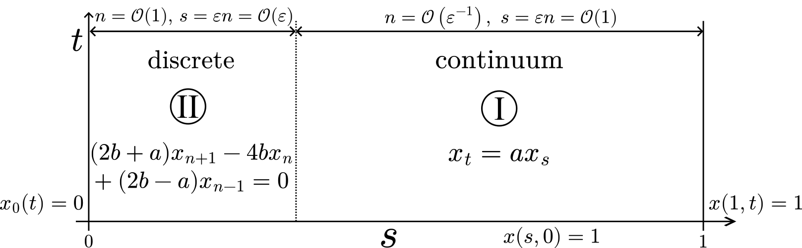
These issues can be resolved by using the method of multiple scales applied to discrete systems, which we discuss in more detail in Section 4. The resolution of these issues in the system (1) for $t=\mathcal{O}(1)$, i.e. neglecting the early time boundary layer to focus on the main point, is that while there are two different asymptotic regions in structure space, only the outer region (Region I in Figure 1) can be represented by a continuum equation. The inner region on the left-hand side of the domain (Region II in Figure 1) is fundamentally discrete. Specifically, in the continuum outer region (Region I), $n=\mathcal{O}\left(\varepsilon^{-1}\right)$ and the leading-order solution is independent of the discrete variable $x_{n}(t)\equiv x(s,t)=x(\varepsilon n,t)$. The dynamics in the outer region are governed by

$$x_{t}=ax_{s},\qquad x(1,t)=1,\qquad x(s,0)=1,$$ (12)

which is solved by

$$x(s,t)=1.$$ (13)

In the fundamentally discrete boundary layer (Region II), $n=\mathcal{O}(1)$ and the leading-order problem is given by

$$(2b+a)x_{n+1}-4bx_{n}+(2b-a)x_{n-1}=0,\qquad x_{0}=0.$$ (14)

Equation 14 is solved by

$$x_{n}=A\left[1-\left(\frac{2b-a}{2b+a}\right)^{-n}\right].$$ (15)

Formally matching the continuum outer region solution (13) to the discrete inner solution (15) yields $A=1$. The resulting composite solution

$$x\sim 1-\left(\frac{2b-a}{2b+a}\right)^{-n}=1-\left(\frac{2b-a}{2b+a}\right)^{-s/\varepsilon}$$ (16)

is asymptotically consistent with Equation 10, demonstrating its improved accuracy over the solution of the truncated PDE (9).

Figure 1: The asymptotic structure of the illustrative example is made of one outer region (I) which can be represented with a continuum structured variable, and one boundary layer (II) which is fundamentally discrete.

3 Model development

We consider a population which exhibits an intrinsic organisation (biological structure) and partition it into discrete classes (mathematical structure), presenting the subsequent model in dimensionless form. In this model, $u_{n}(t)\geq 0$ is the dimensionless density of the subpopulation with structure level $n\in\{0,1,\dots,N\}$ at time $t$.

We consider a model where transitions between neighbouring subpopulations occur at rates $Nk_{n}^{+}(t)$ and $Nk_{n}^{-}(t)$ (see Figure 2).

Figure 2: Schematic of forward and backward transitions of neighbouring subpopulations with their respective rates, for $n=1,\dots,N-1$.

We impose

$$k_{N}^{+}(t)\equiv 0,\qquad k_{0}^{-}(t)\equiv 0,$$ (17)

which ensures that there are no forward transitions by individuals with $n=N$, and no backwards transitions by individuals with $n=0$, respectively. We also assume that transitions to higher structure levels become progressively more difficult at higher levels, while transitions to lower levels are increasingly more difficult at lower levels, corresponding to $k_{n}^{+}(t)$ and $k_{n}^{-}(t)$ being monotonically decreasing and increasing in $n$, respectively. In this model, we assume further that recruitment is restricted to the endpoints $n=0$ and $n=N$, where it occurs at rates $f(t)$ and $g(t)$, respectively, outlining the more general case of global recruitment in the discussion. Finally, we suppose that individuals with structure level $n$ are removed (via e.g. death or emigration) at rate $\beta_{n}(t)>0$. For $t>0$, our governing equations are

$$\frac{\mathrm{d}u_{0}}{\mathrm{d}t} =\underbrace{f(t)}_{\text{recruitment at }n=0}-\,Nk_{0}^{+}u_{0}+Nk_{1}^{-}u_{1}-\beta_{0}u_{0},$$ (18a)

$$\frac{\mathrm{d}u_{n}}{\mathrm{d}t} =\underbrace{N\left[k_{n-1}^{+}u_{n-1}-k_{n}^{+}u_{n}\right]}_{\text{forward transition}}+\underbrace{N\left[k_{n+1}^{-}u_{n+1}-k_{n}^{-}u_{n}\right]}_{\text{backward transition}}-\underbrace{\beta_{n}u_{n}}_{\text{removal}},\quad 1\leq n\leq N-1$$ (18b)

$$\frac{\mathrm{d}u_{N}}{\mathrm{d}t} =\underbrace{g(t)}_{\text{recruitment at }n=N}+\,Nk_{N-1}^{+}u_{N-1}-Nk_{N}^{-}u_{N}-\beta_{N}u_{N}.$$ (18c)

A key assumption for our upscaling is that the functions $k_{n}^{+},k_{n}^{-},\beta_{n}$ are well-defined and continuous in $nN^{-1}$, with bounded gradients as $N\to\infty$. That is, these functions vary slowly in $n$ and, for $N\gg 1$, can be approximated by functions of $t$ and

$$s:=nN^{-1},$$ (19)

so we may write

$$h_{n}(t)\equiv h(s,t)=h(nN^{-1},t),$$ (20)

for $h\in\{k^{+},k^{-},\beta\}$. Then Equation 17 gives

$$k^{+}(1,t)\equiv 0,\qquad k^{-}(0,t)\equiv 0.$$ (21)

Given continuity, these functions are small close to their vanishing points. That is, we have

$$k^{+}=o(1)\quad\text{for}\,\,N-n=\mathcal{O}(1),\qquad k^{-}=o(1)\quad\text{for}\,\,n=\mathcal{O}(1).$$ (22)

We further assume that they are not small away from these points

$$k^{+},k^{-}=\mathcal{O}(1),$$ (23)

and that $\beta,f,g=\mathcal{O}(1)$ within the full state space.

We close the model (18) by imposing the following initial conditions

$$u_{n}(0)=U_{n}\geq 0,\quad 0\leq n\leq N.$$ (24)

We assume that the sum of the initial distribution, $\sum_{n=0}^{N}U_{n}$, is independent of $N$, implying that the initial mass of the system remains finite, so that refining the discretisation does not alter the total mass. We also assume that $U_{n}$ represents samples from a smooth profile, so that it varies slowly with respect to $n$. For $N\gg 1$, it can therefore be approximated by a function of the continuous variable $s$ (defined in LABEL:eq:definition_of_\cvar), namely

$$U_{n}\equiv U(s)=U\left(nN^{-1}\right).$$ (25)

We make this assumption for simplicity; however, the analysis can be extended to initial conditions that are non-smooth in $s$.

3.1 Numerical simulations: linear neighbouring transition rates

To gain some intuition into the form of solutions to (18), we first present some numerical simulations. We consider a system with linear functional forms for $k_{n}^{+}$ and $k_{n}^{-}$, and constant values for $f,g$ and $\beta_{n}$:

$$k_{n}^{+}(t)=k_{f}\left(1-\frac{n}{N}\right),\quad k_{n}^{-}(t)=k_{b}\left(\frac{n}{N}\right),\quad f(t)=\frac{1}{2},\quad g(t)=0,\quad\beta_{n}(t)=\gamma.$$ (26)

Here, $k_{f},k_{b}$ and $\gamma$ are non-negative parameters. We impose uniform initial conditions so that $u_{n}(0)=N^{-1}$ for $0\leq n\leq N$.

Figure 3: Distributions of the discretely structured population, $u_{n}(t)$ for $n=0,1,\dots,N$ found by solving Equations 18 and 26 for $N=10,50,100,500$ at times $t=0.1,0.5,2,25$ when $k_{f}=1,k_{b}=0.5,\gamma=1.25$ and $u_{n}(0)=N^{-1}$ for all $n$. For $N=500$, we highlight the apparent moving wavefronts with arrows.

We use the ode45 routine in MATLAB with $N=10,50,100$ and $500$ to construct numerical simulations to Equation 18 with functional forms given by Equation 26. The illustrative results in Figure 3 show the population distribution at early times ($t=0.1$), two intermediate times ($t=0.5,2$) and at longer times ($t=25$). For fixed $N$, the distribution appears to evolve in a wave-like manner. That is, two waves appear to propagate from each endpoint in structure space, heading towards an interior point where they coalesce (see arrows for $N=500$). Moreover, we can identify regions of rapid variation throughout, while the distributions appear to be sufficiently continuous to allow a clear interpolation. As $N$ increases, regions of fast variation become sharper, indicating that there may be interior boundary layers for $N\gg 1$. The dynamics at early times ($t=0.1$) reveal a rapid variation in the distribution at the endpoints, suggesting the presence of two boundary layers also at the endpoints.

4 Discrete-to-continuum approximation

In this section, we derive a uniformly valid continuum approximation to the general discrete structured model (18) for large $N\gg 1$. We transform the discrete distribution $u_{n}(t),n=0,1,\dots,N$, to a continuous function $u(s,t)$ defined over a continuous structure variable $s$. We combine the method of multiple scales with matched asymptotic expansions, both applied to discrete systems, as used in for example (17). The key steps are:

1. Introduce two length scales: a short discrete scale and a long continuum scale.

2. Assume dependence of the solution $u$ on both scales. The extra degree of freedom this introduces will be removed later in Step 6, in the usual manner for the standard method of multiple scales.

3. Self-consistently expand in both the discrete and continuum variables.

4. Construct an asymptotic expansion for $u$ in $N^{-1}\ll 1$.

5. Solve the leading-order problem and identify a short-scale periodicity.

6. Apply the Fredholm Alternative Theorem with the short-scale periodicity to obtain a solvability condition. This is the requisite upscaled PDE.

In our setting, the discrete class variable $n$ naturally plays the role of the short scale, capturing the fine‐scale variation across neighbouring classes. We introduce a corresponding continuum long scale by defining $s$ as in LABEL:eq:definition_of_\cvar, and set $\varepsilon=N^{-1}$ to obtain

$$s=\varepsilon n,$$ (27)

considering $s$ to vary smoothly over the interval $[0,1]$ as $n$ ranges from $0$ to $N$. We then regard the solution to depend simultaneously on both variables, writing

$$u_{n}(t)\equiv u_{n}(s,t)=u_{n}(\varepsilon n,t).$$ (28)

In our model, 1-periodicity arises at leading-order. Further details on the discrete multiple scales approach and additional applications for its use can be found in (18, 17).

4.1 Asymptotic structure

Before presenting the technical details of our upscaling, it is helpful to briefly outline the asymptotic structure we identify and subsequently analyse. We illustrate schematically this asymptotic structure in Figure 4. As can be seen in the numerical simulations, three inner boundary layers (regions IN1, IN2 and IN3) separate four outer regions (regions O1, O2, O3 and O4), and there are two additional boundary layers at the left and right endpoints (regions B1 and B2). Additional asymptotic regions will arise when these boundary layers overlap, but for brevity we do not investigate those here. As $t$ increases, the three inner boundary layers start to intersect, forming a transient overlap region (region IN4) that separates outer regions O1 and O4, and which eventually reduces to a single inner layer (region IN5). Moreover, for early times, the boundary layer at the left endpoint intersects the inner boundary layer at the left wavefront, forming region B3 (with similar for region B4 on the right-hand side of the domain).

Below, we start by deriving the continuum approximation in the outer regions. Then, we focus on the boundary layers at the domain endpoints to derive appropriate boundary conditions for the continuum problem. Finally, we conduct boundary layer analyses within the inner boundary layers to close the continuum problem.

Figure 4: (a) The asymptotic regions we investigate in this paper, via the multiple scales analysis in Sections 4.2, 4.3, 4.4, 4.5, 4.6 and 4.7. The outer regions (white, O1–O4) are governed by continuum equations (40), while the shaded zones correspond to boundary layers where the dynamics change character. At the domain endpoints, boundary layers B1 and B2 arise; because transitions here are of the same order as the discrete structure, these regions are fundamentally discrete and cannot be described by a continuum approximation. Within the interior, a stagnation point at $s=c(t)$ (Equation 53) generates an inner moving boundary layer (region IN1), while moving fronts at $s=\ell(t)$ (Equation 69) and $s=r(t)$ (Equation 74) generate additional inner layers (regions IN2 and IN3). (b) Additional asymptotic regions arise due to the intersections of various boundary layers, which we do not investigate in this paper. At early times, the inner boundary layer at the left wavefront intersects the boundary layer at the left endpoint, forming region B3. Similarly, region B4 arises from the right endpoint-wavefront intersection. As time evolves, the three inner layers intersect to form a transient overlap region (region IN4), which eventually coalesce into a single steady-state inner layer (region IN5).

4.2 Outer regions

We first consider the outer regions away from the endpoints at $n=0,N$, where $\varepsilon n,1-\varepsilon n=\mathcal{O}(1)$. In these outer regions, the system dynamics are given by Equation 18b. We apply the discrete method of multiple scale by following Steps 1-6 specified at the beginning of Section 4.

Step 1.
Using the method of multiple scales applied to discrete systems, we introduce $s=\varepsilon n\in(0,1)=\mathcal{O}(1)$ (defined in LABEL:eq:definition_of_\cvar) as the continuum scale.

Step 2.
We assume that the solution $u_{n}$ to Equation 18 depends on both the discrete and continuum scales:

$$u_{n}(t)\equiv u_{n}(s,t)=u_{n}(\varepsilon n,t).$$ (29)

Moreover, from Equation 20 we have

$$k_{n}^{+}(t)\equiv k^{+}(s,t)=k^{+}(\varepsilon n,t),\,\,k_{n}^{-}(t)\equiv k^{-}(s,t)=k^{-}(\varepsilon n,t),\,\,\beta_{n}(t)\equiv\beta(s,t)=\beta(\varepsilon n,t).$$ (30)

Step 3.
We self-consistently expand in the discrete and continuum variables. Specifically, we have

$$u_{n\pm 1}(\varepsilon n\pm\varepsilon,t) =u_{n\pm 1}(s\pm\varepsilon,t)=u_{n\pm 1}(s,t)\pm\varepsilon\frac{\partial u_{n\pm 1}}{\partial s}(s,t)+\mathcal{O}(\varepsilon^{2}),$$ (31a)

$$k^{+}(\varepsilon n-\varepsilon,t) =k^{+}(s-\varepsilon,t)=k^{+}(s,t)-\varepsilon\frac{\partial k^{+}}{\partial s}(s,t)+\mathcal{O}(\varepsilon^{2}),$$ (31b)

$$k^{-}(\varepsilon n+\varepsilon,t) =k^{-}(s+\varepsilon,t)=k^{-}(s,t)+\varepsilon\frac{\partial k^{-}}{\partial s}(s,t)+\mathcal{O}(\varepsilon^{2}).$$ (31c)

Substituting Equation 31 into Equation 18b, we obtain

$$\frac{\partial u_{n}}{\partial t} =\frac{1}{\varepsilon}\left[\left(k^{+}-\varepsilon\frac{\partial k^{+}}{\partial s}\right)\left(u_{n-1}-\varepsilon\frac{\partial u_{n-1}}{\partial s}\right)-k^{+}u_{n}\right]$$

$$+\frac{1}{\varepsilon}\left[\left(k^{-}+\varepsilon\frac{\partial k^{-}}{\partial s}\right)\left(u_{n+1}+\varepsilon\frac{\partial u_{n+1}}{\partial s}\right)-k^{-}u_{n}\right]-\beta u_{n}+\mathcal{O}(\varepsilon).$$ (32)

In Equation 32 we have omitted the function arguments for notational brevity; but here, and hereafter, $u_{n},k^{\pm}$ and $\beta$ are evaluated at $(s,t)$ unless otherwise specified.

Step 4.
We expand $u_{n}(s,t)$ as an asymptotic series:

$$u_{n}(s,t)=\varepsilon u_{n}^{(0)}(s,t)+\varepsilon^{2}u_{n}^{(1)}(s,t)+\mathcal{O}(\varepsilon^{3}),$$ (33)

where $u_{n}^{(i)}=\mathcal{O}(1)$. The leading-order scaling in Equation 33 ensures that the mass of the system is independent of $N=\varepsilon^{-1}$ as $N\to\infty$. Substituting Equation 33 into Equation 32, we obtain

$$\varepsilon\frac{\partial u_{n}^{(0)}}{\partial t}= \left[k^{+}\left(u_{n-1}^{(0)}-u_{n}^{(0)}\right)+k^{-}\left(u_{n+1}^{(0)}-u_{n}^{(0)}\right)\right]$$

$$+\varepsilon\left[k^{+}\left(-\frac{\partial u_{n-1}^{(0)}}{\partial s}+u_{n-1}^{(1)}-u_{n}^{(1)}\right)-\frac{\partial k^{+}}{\partial s}u_{n-1}^{(0)}\right.$$

$$\left.+k^{-}\left(\frac{\partial u_{n+1}^{(0)}}{\partial s}+u_{n+1}^{(1)}-u_{n}^{(1)}\right)+\frac{\partial k^{-}}{\partial s}u_{n+1}^{(0)}-\beta u_{n}^{(0)}\right]+\mathcal{O}(\varepsilon^{2}).$$ (34)

Equating the $\mathcal{O}\left(1\right)$ terms in Equation 34 yields

$$0=k^{+}\left(u_{n-1}^{(0)}-u_{n}^{(0)}\right)+k^{-}\left(u_{n+1}^{(0)}-u_{n}^{(0)}\right).$$ (35)

Step 5.
The general solution to the linear discrete equation (35) is

$$u_{n}^{(0)}(s,t)=A(s,t)+B(s,t)\left(\frac{k^{+}}{k^{-}}\right)^{n},$$ (36)

recalling that $n=\mathcal{O}(\varepsilon^{-1})$. We will see in Section 4.6 that it is not asymptotically consistent to have leading-order solutions that vary exponentially in the short scale $n$ across the outer regions. Therefore, we require $B(s,t)=0$ and

$$u_{n}^{(0)}(s,t)=A(s,t):=u(s,t),$$ (37)

where we redefine $A$ as $u$ for notational clarity. We conclude that neighbouring populations are independent of the discrete variable $n$ at leading order, and so in these outer regions any variation in the structured variable occurs over the slow continuum scale $s$. Importantly for the method of multiple scales, we note that the leading-order solution (37) is 1-periodic in the short scale $n$. Our remaining task is to understand how the leading-order solution $u(s,t)$ depends on the long scale $s$ and time $t$. To do this, we must proceed to higher orders.

Step 6.
At $\mathcal{O}(\varepsilon)$ in Equation 34, we have

$$\frac{\partial u}{\partial t}=\frac{\partial}{\partial s}\left[\left(k^{-}-k^{+}\right)u\right]-\beta u+k^{+}\left(u_{n-1}^{(1)}-u_{n}^{(1)}\right)+k^{-}\left(u_{n+1}^{(1)}-u_{n}^{(1)}\right).$$ (38)

Applying the Fredholm Alternative Theorem for linear difference operators, we impose the method of multiple scales constraint of 1-periodicity in the short scale (which, together with the leading-order periodicity, maintains uniform validity of the asymptotic expansion). This yields

$$u_{n}^{(1)}(s,t)=u^{(1)}(s,t),$$ (39)

so that the first-order correction of the structured model is also independent of the discrete variable $n$. Under these conditions, the corresponding solvability condition is given by

$$\frac{\partial u}{\partial t}=\frac{\partial}{\partial s}\left[\left(k^{-}-k^{+}\right)u\right]-\beta u,$$ (40)

where $k^{\pm}=k^{\pm}(s,t)$. We present a more detailed derivation of the appropriate solvability condition in terms of suitable inner products and adjoints in Appendix A.

The hyperbolic, advection-dominated PDE (40) governs the leading-order dynamics of the structured population in the outer regions. To close Equation 40, we require appropriate boundary and initial conditions. The initial conditions are

$$u(s,0)=U(s),$$ (41)

where $U(s)$ is given by Equations 24 and 25.

However, at this stage, we do not have enough information to determine the boundary conditions for Equation 40. Given that Equation 40 is a first-order PDE, we might expect that one boundary condition would suffice. However, information propagates along the characteristics that emerge from the left boundary ($s=n=0$) to the right, and vice versa from the right boundary ($s=1$ or $n=N$). Figure 5 illustrates the transition rates $k^{+}$ and $k^{-}$ as functions of the continuum variable $s$, highlighting how they determine the direction in which information propagates along the characteristics. Therefore two boundary conditions are needed: one associated with the region influenced by characteristics originating at the left boundary, the other with the region influenced by characteristics originating at the right. We derive the appropriate boundary conditions by analysing additional boundary layers at the endpoints of the domain (see also the numerical simulations in Figure 3 at $t=0.1$). These asymptotic regions are fundamentally discrete, in that continuum representations are not appropriate therein, as we will show in Section 4.3. Nevertheless, by matching the discrete problems in these boundary layers to the continuum outer regions, we can derive consistent boundary conditions for the outer problems.

Figure 5: Illustrative sketch showing $k^{+}$ and $k^{-}$ against $s$. Monotonicity with respect to $n$ imply that $k^{+}$ and $k^{-}$ must intersect at a unique interior point in the continuum state space. At this point, the advection term in Equation 40 is zero and the PDE becomes degenerate.

We also note that the coefficient of the advective term vanishes in the interior of the domain, at the unique location where $k^{+}=k^{-}$ (see Figure 5) and the characteristics seem to meet. At this point, the advective term in Equation 40 vanishes and the PDE appears to be degenerate. We will return to this degeneracy in Section 4.6, where we investigate the inner boundary layer around this point.

4.3 Boundary layer at the left endpoint

We first investigate the asymptotic region near $n=0$. A classic Taylor expansion method might suggest a natural approach for investigating the boundary layer in the continuum variable $s$, as for standard PDEs. However, the appropriate scaling would be $s=\mathcal{O}(\varepsilon)$, which corresponds to $n=\mathcal{O}(1)$. As such, it is not consistent to treat $s=\varepsilon n$ as a continuum variable in this region. The system is fundamentally discrete in this region, where it is governed by Equation 18b with $n=\mathcal{O}(1)$. However, since the coefficients still vary slowly, and we are effectively zooming into a short scale in this region, we may self-consistently expand Equation 20 as follows

$$k^{\pm}_{n}(t) \equiv k^{\pm}(\varepsilon n,t)=k^{\pm}(0,t)+\varepsilon n\frac{\partial k^{\pm}}{\partial s}(0,t)+\mathcal{O}(\varepsilon^{2}),$$ (42a)

$$k_{n-1}^{+}(t) \equiv k^{+}(\varepsilon n-\varepsilon,t)=k^{+}(0,t)+(\varepsilon n-\varepsilon)\frac{\partial k^{+}}{\partial s}(0,t)+\mathcal{O}(\varepsilon^{2}),$$ (42b)

with the equivalent for $k_{n+1}^{-}$ and $\beta_{n}$. Additionally, in this boundary layer we still expand $u_{n}(t)$ as an asymptotic series:

$$u_{n}(t)=\varepsilon u_{n}^{(0)}(t)+\varepsilon^{2}u_{n}^{(1)}(t)+\mathcal{O}(\varepsilon^{3}).$$ (43)

Substituting Equations (21), (42), (43) into Equation 18b, we obtain for $n\geq 1$

$$\varepsilon\frac{\mathrm{d}u_{n}^{(0)}}{\mathrm{d}t} =\frac{1}{\varepsilon}\left[\left(k^{+}(0)+(\varepsilon n-\varepsilon)\frac{\partial k^{+}}{\partial s}(0)\right)\left(\varepsilon u_{n-1}^{(0)}+\varepsilon^{2}u_{n-1}^{(1)}\right)\right.$$

$$\quad\quad\quad-\left.\left(k^{+}(0)+\varepsilon n\frac{\partial k^{+}}{\partial s}(0)\right)\left(\varepsilon u_{n}^{(0)}+\varepsilon^{2}u_{n}^{(1)}\right)\right]$$

$$\quad+\frac{1}{\varepsilon}\left[\left(\varepsilon n+\varepsilon\right)\frac{\partial k^{-}}{\partial s}(0)\left(\varepsilon u_{n+1}^{(0)}+\varepsilon^{2}u_{n+1}^{(1)}\right)-\varepsilon n\frac{\partial k^{-}}{\partial s}(0)\left(\varepsilon u_{n}^{(0)}+\varepsilon^{2}u_{n}^{(1)}\right)\right]$$

$$\quad-\left(\beta(0)+\varepsilon n\frac{\partial\beta}{\partial s}(0)\right)\left(\varepsilon u_{n}^{(0)}+\varepsilon^{2}u_{n}^{(1)}\right)+\mathcal{O}(\varepsilon^{2}),$$ (44)

where we have omitted explicit dependence on $t$ for notational brevity. Since $k^{+},k^{-}$ have bounded gradients as $\varepsilon\to 0$, we have $\frac{\partial k^{\pm}}{\partial s}(0)=\mathcal{O}(1)$. Thus, at $\mathcal{O}(1)$, for $t>0$,

$$0=k^{+}(0,t)\left[u_{n-1}^{(0)}(t)-u_{n}^{(0)}(t)\right],$$ (45)

which gives for $n\geq 1$

$$u_{n-1}^{(0)}(t)=u_{n}^{(0)}(t)=:u_{\text{left}}(t).$$ (46)

In particular, for $n=1$ this gives $u^{(0)}_{0}(t)=u^{(0)}_{1}(t)=u_{\text{left}}(t)$.

Equation 18a defines the dynamics of $u_{0}$, which, given the asymptotic expansion (43) and Equation 17, becomes

$$\varepsilon\frac{\mathrm{d}u^{(0)}_{0}}{\mathrm{d}t}=f(t)-k_{0}^{+}\left(u^{(0)}_{0}+\varepsilon u^{(1)}_{0}\right)+k_{1}^{-}\left(u_{1}^{(0)}+\varepsilon u_{1}^{(1)}\right)-\varepsilon\beta_{0}u^{(0)}_{0}+\mathcal{O}(\varepsilon^{2}).$$ (47)

Equations (22)-(23) imply that $k_{0}^{+}=\mathcal{O}(1),k_{1}^{-}=o(1)$. Hence using Equation 46 in Equation 47 yields at leading-order

$$u_{\text{left}}(t)=\frac{f(t)}{k_{0}^{+}(t)}.$$ (48)

To obtain the appropriate effective boundary condition for the PDE (40) as $s\to 0^{+}$, we must match with Equation 48 for large $n$. This yields the effective condition

$$u(0,t)=\frac{f(t)}{k_{0}^{+}(t)}.$$ (49)

4.4 Boundary layer at the right endpoint

In a similar manner, the region near the right endpoint $n=N$ is fundamentally discrete and cannot be approximated by a continuum representation. We consider this region by setting $n=N-\hat{n}=\varepsilon^{-1}-\hat{n}$ where $\hat{n}=\mathcal{O}(1)$. The analysis follows that in Section 4.3, resulting in the leading-order solution

$$u_{\text{right}}(t):=u^{(0)}_{N}(t)=\frac{g(t)}{k_{N}^{-}(t)}.$$ (50)

Matching with the outer solution as $s\to 1^{-}$ gives the effective boundary condition

$$u(1,t)=\frac{g(t)}{k_{N}^{-}(t)}.$$ (51)

4.5 Effective boundary conditions for the outer PDE

Taken together, Equations 49 and 51 define two boundary conditions for Equation 40 at $s=0,1$. In the left outer region (region O1, in Figure 4a), characteristics propagate rightward from $s=0$. In the right outer region (region O4, in Figure 4a), they propagate leftward from $s=1$. In regions O2 and O3 the characteristics emanate from the initial conditions. The characteristic projections from the outer PDE (40) intersect where $k^{+}=k^{-}$. This constitutes a stagnation point of the outer PDE, where the coefficient of the advective term in Equation 40 vanishes. Any apparent discontinuity at this stagnation point in the outer PDE solution is smoothed by an internal boundary layer (region IN1, in Figure 4a). Moreover, if there is a discontinuity between the boundary condition at $s=0$ and the initial condition for $n=0$, i.e. if

$$\frac{f(0)}{k_{0}^{+}(0)}\neq U_{0},$$ (52)

then the discontinuity propagates along the characteristic projection passing through $(s,t)=(0,0)$, which we identify as the left wavefront (region IN2, in Figure 4a). Given this discontinuity at $t=0$, there is also an early-time boundary layer, which we do not consider here to focus on the main point. Similarly, any discontinuity between the boundary condition at $s=1$ and the initial condition for $n=N$ $\left(\frac{g(0)}{k_{N}^{-}(0)}\neq U_{N}\right)$ propagates through the characteristic projection passing through $(s,t)=(1,0)$ (right wavefront, region IN3 in Figure 4a). We investigate the dynamics in these three regions by performing an inner boundary layer analysis.

4.6 Inner boundary layer at the stagnation point

From Equation 40 we see that the characteristic projections emanating from the left and right endpoints intersect at an interior point $s=c(t)$, defined via

$$k^{-}\big(c(t),t\big)=k^{+}\big(c(t),t\big).$$ (53)

Here, the coefficient of the advective term in Equation 40 vanishes, and the PDE becomes degenerate. Thus, $s=c(t)$ constitutes a stagnation point. In this section, we investigate the system dynamics in the boundary layer that surrounds this degenerate point. Importantly, we proceed using a multiple scales analysis directly on the underlying discrete system (rather than the outer PDE) to ensure that we retain the appropriate information at leading order.

Given that this boundary layer moves in time, different types of behaviour are possible depending on the relative magnitude of its motion. To this end, we introduce $\omega$ to represent the magnitude of the boundary layer motion, writing $c=c(\omega t)$. In order for the outer analysis to remain unmodified, we require $\omega\ll 1$. We will find that the distinguished asymptotic limit which self-consistently incorporates as many mathematical terms as possible (and therefore allows us to tackle all possible behaviours at once) is $\omega=\mathcal{O}(\sqrt{\varepsilon})$. We therefore use this asymptotic size of $\omega$ henceforth. We emphasize that the benefit of considering the distinguished asymptotic limit is that different asymptotic sizes of $\omega$ can be considered subsequently as sublimits of this distinguished limit.

The appropriate scaling for the interior layer around the stagnation point is

$$n=\frac{c(\omega t)}{\varepsilon}+\frac{\tilde{s}}{\sqrt{\varepsilon}}\quad\Rightarrow\quad\tilde{s}=\sqrt{\varepsilon}\left(n-\frac{c(\omega t)}{\varepsilon}\right),$$ (54)

where $n-c/\varepsilon=\mathcal{O}(1/\sqrt{{\varepsilon}})$, so that $\tilde{s}=\mathcal{O}(1)$ is the long scale (continuum variable) in this inner region, and $c(t)=\mathcal{O}(1)$.

Assuming dependence of the solution on both the discrete and continuum scales, as per Step 2 of the method of multiple scales applied to discrete systems, gives

$$u_{n}(t)\equiv u_{n}(\tilde{s},t)=u_{n}\left(\sqrt{\varepsilon}\left(n-\frac{c}{\varepsilon}\right),t\right).$$ (55)

Hence the short variable $n\rightarrow n+1$ implies $\tilde{s}\rightarrow\tilde{s}+\sqrt{\varepsilon}$. The time derivative is transformed using Equation 54 and the chain rule:

$$\frac{\partial}{\partial t}\rightarrow\frac{\partial}{\partial t}-\frac{\omega\dot{c}}{\sqrt{\varepsilon}}\frac{\partial}{\partial\tilde{s}},$$ (56)

where the dot represents differentiation with respect to time. Self-consistently expanding $u_{n\pm 1}(t)$ and using a Taylor series expansion in $\tilde{s}$, we obtain

$$u_{n\pm 1}(t)=u_{n\pm 1}(\tilde{s}\pm\sqrt{\varepsilon},t)=u_{n\pm 1}(\tilde{s},t)\pm\sqrt{\varepsilon}\frac{\partial u_{n\pm 1}}{\partial\tilde{s}}(\tilde{s},t)+\frac{\varepsilon}{2}\frac{\partial^{2}u_{n\pm 1}}{\partial\tilde{s}^{2}}(\tilde{s},t)+\mathcal{O}\left(\varepsilon^{3/2}\right).$$ (57)

Recall from Equation 20 that $k_{n}^{\pm},\beta_{n}$ vary slowly in the discrete variable, and, as such, are functions of $(\varepsilon n,t)$ alone (i.e. they are independent of the short scale $n$ under the method of multiple scales framework). Thus, self-consistently expanding using Equations (53)-(54) and a Taylor series expansion yield

$$k_{n}^{\pm}\equiv k^{\pm}(\varepsilon n)=k^{\pm}\left(c+\sqrt{\varepsilon}\tilde{s}\right) =k^{\pm}_{c}+\sqrt{\varepsilon}\,\tilde{s}\,\partial^{1}k^{\pm}_{c}+\frac{\varepsilon\tilde{s}^{2}}{2}\partial^{2}k^{\pm}_{c}+\mathcal{O}\left(\varepsilon^{3/2}\right),$$ (58a)

$$k_{n-1}^{+}\equiv k^{+}(\varepsilon n-\varepsilon) =k^{+}\left(c+\sqrt{\varepsilon}\,\tilde{s}-\varepsilon\right)$$

$$=k^{+}_{c}+\left(\sqrt{\varepsilon}\,\tilde{s}-\varepsilon\right)\partial^{1}k^{+}_{c}+\frac{\varepsilon\tilde{s}^{2}}{2}\partial^{2}k^{+}_{c}+\mathcal{O}\left(\varepsilon^{3/2}\right),$$ (58b)

$$k_{n+1}^{-}\equiv k^{-}(\varepsilon n+\varepsilon) =k^{-}\left(c+\sqrt{\varepsilon}\,\tilde{s}+\varepsilon\right)$$

$$=k^{-}_{c}+\left(\sqrt{\varepsilon}\,\tilde{s}+\varepsilon\right)\partial^{1}k^{-}_{c}+\frac{\varepsilon\tilde{s}^{2}}{2}\partial^{2}k^{-}_{c}+\mathcal{O}\left(\varepsilon^{3/2}\right),$$ (58c)

$$\beta_{n}\equiv\beta(\varepsilon n)=\beta\left(c+\sqrt{\varepsilon}\tilde{s}\right) =\beta_{c}+\mathcal{O}\left(\sqrt{\varepsilon}\right),$$ (58d)

where we omit the time dependence in the arguments for notational brevity. Here, we define

$$k^{\pm}_{c}:=k^{\pm}(c(\omega t),t), \partial^{p}k^{\pm}_{c}:=\frac{\partial^{p}k^{\pm}}{\partial s^{p}}(c(\omega t),t)\,\,\text{for}\,\,p=1,2, \beta_{c}:=\beta(c(\omega t),t).$$ (59)

Moreover, since $k^{+},k^{-}$ have bounded gradients in the limit $\varepsilon\to 0$, we have $\partial^{p}k^{\pm}_{c}=\mathcal{O}(1)$.

Substituting Equations 57 and 58 into Equation 18b, we obtain

$$\frac{\partial u_{n}}{\partial t}-\frac{\omega\dot{c}}{\sqrt{\varepsilon}}\frac{\partial u_{n}}{\partial\tilde{s}} =\frac{1}{\varepsilon}\left[\left(k^{+}_{c}+(\sqrt{\varepsilon}\,\tilde{s}-\varepsilon)\partial^{1}k^{+}_{c}+\frac{\varepsilon\tilde{s}^{2}}{2}\partial^{2}k^{+}_{c}\right)\left(u_{n-1}-\sqrt{\varepsilon}\frac{\partial u_{n-1}}{\partial\tilde{s}}\right.\right.$$

$$\quad\quad\quad+\left.\left.\frac{\varepsilon}{2}\frac{\partial^{2}u_{n-1}}{\partial\tilde{s}^{2}}\right)-\left(k^{+}_{c}+\sqrt{\varepsilon}\,\tilde{s}\,\partial^{1}k^{+}_{c}+\frac{\varepsilon\tilde{s}^{2}}{2}\partial^{2}k^{+}_{c}\right)u_{n}\right]$$

$$+\frac{1}{\varepsilon}\left[\left(k^{-}_{c}+(\sqrt{\varepsilon}\,\tilde{s}+\varepsilon)\partial^{1}k^{-}_{c}+\frac{\varepsilon\tilde{s}^{2}}{2}\partial^{2}k^{-}_{c}\right)\left(u_{n+1}+\sqrt{\varepsilon}\frac{\partial u_{n+1}}{\partial\tilde{s}}\right.\right.$$

$$\quad\quad\quad+\left.\frac{\varepsilon}{2}\frac{\partial^{2}u_{n+1}}{\partial\tilde{s}^{2}}\right)-\left.\left(k^{-}_{c}+\sqrt{\varepsilon}\,\tilde{s}\,\partial^{1}k^{-}_{c}+\frac{\varepsilon\tilde{s}^{2}}{2}\partial^{2}k^{-}_{c}\right)u_{n}\right]$$

$$-\beta_{c}u_{n}+\mathcal{O}\left(\sqrt{\varepsilon}\right).$$ (60)

We expand $u_{n}(\tilde{s},t)$ as the asymptotic expansion

$$u_{n}(\tilde{s},t)=u_{n}^{(0)}(\tilde{s},t)+\sqrt{\varepsilon}\,u_{n}^{(1/2)}(\tilde{s},t)+\varepsilon\,u_{n}^{(1)}(\tilde{s},t)+\mathcal{O}(\varepsilon^{3/2}).$$ (61)

Substituting Equation 61 into Equation 60, at $\mathcal{O}(1/\varepsilon)$ we obtain

$$0=k^{+}_{c}(t)\left[u_{n-1}^{(0)}(\tilde{s},t)-u_{n}^{(0)}(\tilde{s},t)\right]+k^{-}_{c}(t)\left[u_{n+1}^{(0)}(\tilde{s},t)-u_{n}^{(0)}(\tilde{s},t)\right].$$ (62)

Given that $k^{+}_{c}=k^{-}_{c}$ at the stagnation point by definition, the general solution to the linear discrete equation (62) is

$$u_{n}^{(0)}(\tilde{s},t)=\tilde{A}(\tilde{s},t)+\tilde{B}(\tilde{s},t)n.$$ (63)

The solution (63) allows for linear growth in $n$ across the inner boundary layer. However, this corresponds to a change in asymptotic magnitude across the boundary layer that is not consistent with the outer equations and boundary conditions. Hence, neighbouring populations in this inner region are independent of the discrete variable $n$ at leading-order in this system. Thus, we require $\tilde{B}(\tilde{s},t)=0$ and

$$u_{n}^{(0)}(\tilde{s},t)=\tilde{A}(\tilde{s},t):=u_{c}(\tilde{s},t),$$ (64)

where we redefine $\tilde{A}$ as $u_{c}$ for later notational clarity. At the next order, recalling that $\omega=\mathcal{O}\left(\sqrt{{\varepsilon}}\right)$, equating the $\mathcal{O}(1/\sqrt{\varepsilon})$ terms in Equation 60 yields

$$0= \left[k^{-}_{c}-k^{+}_{c}\right]\frac{\partial u_{c}}{\partial\tilde{s}}+k^{+}_{c}\left[u_{n-1}^{(1/2)}-u_{n}^{(1/2)}\right]+k^{-}_{c}\left[u_{n+1}^{(1/2)}-u_{n}^{(1/2)}\right].$$ (65)

Since $k^{-}_{c}=k^{+}_{c}$ in the boundary layer (Equation 53) and imposing the method of multiple scales constraint of periodicity on the short scale, we deduce from Equation 65 that the solution is also independent of $n$ at this order i.e.

$$u_{n}^{(1/2)}(\tilde{s},t)=u_{c}^{(1/2)}(\tilde{s},t).$$ (66)

Finally, at $\mathcal{O}(1)$ in Equation 60 we have

$$\frac{\partial u_{c}}{\partial t}-\frac{\omega\dot{c}}{\sqrt{{\varepsilon}}}\frac{\partial u_{c}}{\partial\tilde{s}}= \left(\partial^{1}k^{-}_{c}-\partial^{1}k^{+}_{c}\right)\frac{\partial}{\partial\tilde{s}}\left(\tilde{s}\,u_{c}\right)+\left(\frac{k^{+}_{c}}{2}+\frac{k^{-}_{c}}{2}\right)\frac{\partial^{2}u_{c}}{\partial\tilde{s}^{2}}-\beta_{c}u_{c}$$

$$+k^{+}_{c}\left[u_{n-1}^{(1)}-u_{n}^{(1)}\right]+k^{-}_{c}\left[u_{n+1}^{(1)}-u_{n}^{(1)}\right],$$ (67)

again using the definition $c$ (Equation 53). Finally, applying the Fredholm Alternative Theorem (see Section 4.2 and Appendix A), leads to the following solvability condition

$$\frac{\partial u_{c}}{\partial t}=\frac{\partial}{\partial\tilde{s}}\left[\frac{1}{2}\left(k^{+}_{c}+k^{-}_{c}\right)\frac{\partial u_{c}}{\partial\tilde{s}}-\left((\partial^{1}k^{+}_{c}-\partial^{1}k^{-}_{c})\tilde{s}-\frac{\omega\dot{c}}{\sqrt{{\varepsilon}}}\right)u_{c}\right]-\beta_{c}u_{c}.$$ (68)

Equation 68 is a parabolic, advection-diffusion PDE which governs the leading-order dynamics of the structured population in the inner (moving) boundary layer around the stagnation point at $s=c(\omega t)$ (region IN1 in Figure 4a). Equation 68 has been derived for the distinguished asymptotic limit where $\omega=\mathcal{O}(\sqrt{\varepsilon})$, and hence all terms contribute at leading order. Different asymptotic scalings of $\omega$ can be derived formally as sublimits of Equation 68. For example, in the sublimit $\omega\ll\sqrt{\varepsilon}$, the $\dot{c}$ term is negligible. In the sublimit $\omega\gg\sqrt{\varepsilon}$, Equation 68 splits into additional asymptotic subregions in which fewer terms balance. The discrete boundary layer analysis in this section, culminating with Equation 68, shows that the apparent degeneracy in the outer continuum approximation is resolved over an inner continuum region. The appropriate boundary conditions for Equation 68 are obtained by matching, and are the limits of the outer solutions as they approach this inner region.

4.7 Inner boundary layers at the wavefronts

As seen in Figure 3, the distribution appears to evolve with wave-like properties, propagating towards the interior point $s=c(t)$ from the left and right boundaries. This is due to discontinuities between the boundary and initial conditions at the left and right boundaries. These discontinuities propagate along the characteristic projections that pass through the left and right endpoints, which we refer to as the left and right wavefronts. In this section, we derive continuum equations that describe the dynamics in the boundary layers at the wavefronts. The position of the left wavefront in the outer system is at $s=\ell(t)$, where, from the continuum outer equation (40),

$$\frac{\mathrm{d}\ell}{\mathrm{d}t}=k^{+}(\ell,t)-k^{-}(\ell,t),\qquad\ell(0)=0.$$ (69)

This characteristic projection partitions the $(s,t)$-plane into two regions, separated by the discontinuity at $(0,0)$ defined in Equation 52. To the right of this characteristic (region O2 in Figure 4a), the characteristic lines emanate from the initial conditions, while to the left (region O1 in Figure 4a), they emanate from the boundary condition at $s=0$. Figure 6 illustrates this behaviour in numerical simulations for the linear case discussed in Section 3.1. The wavefronts are the locations in structure space where the population distribution changes rapidly.

The analysis in the boundary layer for the left wavefront is similar to that presented in Section 4.6, with the same scaling for the long variable, but now with distinguished limit $\omega=\mathcal{O}(1)$

$$\hat{s}=\sqrt{\varepsilon}\left(n-\frac{\ell(t)}{\varepsilon}\right).$$ (70)

Since we are now moving with the separating characteristic via Equation 69, we can set $\omega=1$ without loss of generality. Then, at $\mathcal{O}(1/\sqrt{\varepsilon})$ we have

$$-\dot{\ell}\frac{\partial u_{\ell}}{\partial\hat{s}}= \left[k^{-}_{\ell}-k^{+}_{\ell}\right]\frac{\partial u_{\ell}}{\partial\hat{s}}+k^{+}_{\ell}\left[u_{n-1}^{(1/2)}-u_{n}^{(1/2)}\right]+k^{-}_{\ell}\left[u_{n+1}^{(1/2)}-u_{n}^{(1/2)}\right]$$

$$+\hat{s}\,u_{\ell}\left(\partial^{1}k^{+}_{\ell}+\partial^{1}k^{-}_{\ell}-\partial^{1}k^{+}_{\ell}-\partial^{1}k^{-}_{\ell}\right),$$ (71)

where $u_{\ell}(\hat{s},t)$ is the continuum density function representing the leading-order dynamics in this inner boundary layer, and

$$k^{\pm}_{\ell}:=k^{\pm}(\ell,t), \partial^{1}k^{\pm}_{\ell}:=\frac{\partial k^{\pm}}{\partial s}(\ell,t), \beta_{\ell}:=\beta(\ell,t).$$ (72)

Given we are moving with a characteristic (69), all terms in Equation 71 involving $u_{\ell}$ vanish (validating the asymptotic scalings employed). Hence, $u_{n}^{(1/2)}$ is 1-periodic. Then proceeding as in Section 4.6, we obtain the following solvability condition

$$\frac{\partial u_{\ell}}{\partial t}=\frac{1}{2}\left(k^{+}_{\ell}+k^{-}_{\ell}\right)\frac{\partial^{2}u_{\ell}}{\partial\hat{s}^{2}}+\left(\partial^{1}k^{-}_{\ell}-\partial^{1}k^{+}_{\ell}\right)\frac{\partial}{\partial\hat{s}}\left(\hat{s}u_{\ell}\right)-\beta_{\ell}u_{\ell}.$$ (73)

The parabolic advection-diffusion PDE (73) defines the leading-order dynamics of the structured population in the inner (moving) boundary layer around the left wavefront at $s=\ell(t)$ (region IN2 in Figure 4a). Our analysis of the discrete system in this boundary layer shows that the apparent discontinuity across this separating characteristic in the outer continuum approximation (40) is smoothed within an inner continuum region via Equation 73. The boundary conditions for Equation 73 are obtained by matching with the solutions in the adjacent outer regions. We also note that $\ell\equiv c$ at steady state, since the same equation is satisfied for $c$ and $\ell$ (see Equations 53 and 69 at steady state), $\dot{c}=0$ and Equations 73 and 68 are identical. Indeed, at steady state, all inner boundary layers coalesce into a single asymptotic region (region IN5 in Figure 4b).

A similar analysis smooths the solution around the right wavefront at $s=r(t)$, where

$$\frac{\mathrm{d}r}{\mathrm{d}t}=k^{+}(r,t)-k^{-}(r,t),\qquad r(0)=1.$$ (74)

This characteristic projection emanates from the right endpoint. The leading-order dynamics in this inner moving boundary layer are also defined by the advection-diffusion PDE (73) with appropriate boundary conditions obtained by matching with the adjacent outer regions.

Figure 6: Distribution $u_{n}(t)$ for $n=0,1,\dots,N$ obtained by solving Equation 18 for $N=500$ with linear functional forms given by Equation 26. The red line shows how the stagnation point $s=c(\omega t)$ (given by Equation 53) moves over time, the green and purple lines show the position of the left wavefront $s=\ell(t)$ (given by Equation 69) and right wavefront $s=r(t)$ (given by Equation 74), respectively, over time. The dynamics are shown at the time points $t=0.1,0.5,2$ and $25$. The initial conditions are taken to be $u_{n}(0)=N^{-1}$ and we set $k_{f}=1,k_{b}=0.5,\gamma=1.25$.

5 Example: early-stage atherosclerosis

We now demonstrate the implications of our analysis for a specific application. The model describes the dynamics of macrophage-lipid interactions during the early stages of atherosclerosis (6). During early atherosclerosis, low-density lipoprotein (LDL) particles penetrate the artery wall, eliciting an inflammatory response and promoting the recruitment of macrophages that engulf LDL (4, 39). In parallel, macrophages offload excess cholesterol to high-density lipoprotein (HDL), which transports LDL out of the lesion (1).

5.1 Continuum approximation

The lipid structured model in (6) decomposes the macrophages into discrete compartments characterised by lipid load. Macrophages move between compartments when they take up and offload lipid. We denote by $u_{n}(t)\geq 0$ the dimensionless concentration of macrophages in the atherosclerotic plaque with $n=0,1,\dots,N$ units of lipid at time $t$, where $N>0$ defines the macrophage lipid capacity. The functions $k_{n}^{+}(t),k_{n}^{-}(t)$ represent the rates of lipid uptake and offloading, respectively, and their functional forms, along with those for the recruitment and removal functions $f(t),g(t),\beta_{n}(t)$, are given in Equation 26. Writing $N=\varepsilon^{-1}$, Equation 20 gives

$$k^{+}(\varepsilon n,t)=k_{f}(1-\varepsilon n), k^{-}(\varepsilon n,t)=k_{b}\varepsilon n, \beta(\varepsilon n,t)=\gamma.$$ (75)

The dynamics in the outer regions are governed by Equation 40 which, for this application, becomes

$$\frac{\partial u}{\partial t}=\frac{\partial}{\partial s}\left[\left(k_{b}s-k_{f}(1-s)\right)u\right]-\gamma u,$$ (76)

with the following boundary conditions, obtained from Equations 49 and 51:

$$u(0,t)=\frac{1}{2k_{f}}, u(1,t)=0.$$ (77)

In the inner region around the stagnation point $s=c(t)$, we deduce from Equation 68 that the dynamics of the macrophage distribution are governed by the following advection-diffusion PDE

$$\frac{\partial u_{c}}{\partial t}=\frac{\partial}{\partial\tilde{s}}\left[\frac{1}{2}\left(k_{f}(1-c)+k_{b}c\right)\frac{\partial u_{c}}{\partial\tilde{s}}+\left((k_{f}+k_{b})\tilde{s}+\frac{\omega\dot{c}}{\sqrt{{\varepsilon}}}\right)u_{c}\right]-\gamma u_{c}.$$ (78)

We note that, given the definition of $c$ (Equation 53) and Equation 75, for this example we have $\dot{c}=0$ for all $t\geq 0$. Figure 6, which presents the lipid distribution with the locations of the inner boundary layers $s=c(t),\ell(t),r(t)$, shows that for $t=0.1,0.5$ the stagnation point is located in a region where the distribution is independent of the structure variable (i.e. it does not lie in a region of rapid variation). We can explain the absence of a shock at $t=0.1,0.5$ by noting that the inner boundary layer IN1 lies between the outer regions O2 and O3 (see Figure 4). In these outer regions, the solution is determined by characteristics originating from the initial condition, which we assumed to be uniform, $u_{n}(0)=N^{-1}$. Consequently, both sides of the inner PDE (78) inherit identical boundary data. Since the boundary conditions coincide, there is no discontinuity and no shock forms. In contrast, for $t=2,25$, the inner region receives boundary data from outer regions O1 and O4. There, the solution is governed by characteristics emanating from the domain boundaries, where the imposed boundary conditions are different. As a result, the two sides of (78) now provide mismatched boundary values, so the inner solution is no longer constant and a shock develops.

In the inner region around the left wavefront $s=\ell(t)$, Equation 73 yields the macrophage dynamics via the following advection-diffusion PDE

$$\frac{\partial u_{\ell}}{\partial t}=\frac{1}{2}\left[k_{f}(1-\ell)+k_{b}\ell\right]\frac{\partial^{2}u_{\ell}}{\partial\hat{s}^{2}}+(k_{f}+k_{b})\frac{\partial}{\partial\hat{s}}\left(\hat{s}u_{\ell}\right)-\gamma u_{\ell},$$ (79)

with equivalent PDE around $s=r(t)$.

5.2 Numerical validation

In Figure 7 we numerically validate the scalings of the inner boundary layers, as identified in Equation 54. We estimate the width of the inner boundary layer by identifying the value of $n$ at which $u_{n}(25)$ attains its maximum value, writing

$$u_{n_{*}}^{\max}:=\max_{n\in[0,1,\dots,N]}u_{n}(25).$$ (80)

The start of the boundary layer is defined as the rightmost point $n=n_{\text{start}}<n_{*}$ at which the distribution has decreased slightly to 98% of this maximum, such that

$$u_{n_{\text{start}}}(25)\leq 0.98u_{n_{*}}^{\max}.$$ (81)

The end of the boundary layer is defined as the leftmost point $n=n_{\text{end}}>n_{*}$ at which the distribution has decayed to 2% of its maximum, i.e.

$$u_{n_{\text{end}}}(25)\leq 0.02u_{n_{*}}^{\max}.$$ (82)

Then, the width of the boundary layer is defined as

$$w_{\varepsilon}:=\varepsilon(n_{\text{end}}-n_{\text{start}}).$$ (83)

Figure 7 shows a plot of $w_{\varepsilon}/\varepsilon^{1/2}$ as $\varepsilon$ varies. As expected from the inner scaling given by Equation 54, the plot is approximately constant in $\varepsilon$ i.e. the width increases linearly with $\varepsilon^{1/2}$.

Figure 7: Plot of $w_{\varepsilon}/\varepsilon^{1/2}$, where $w_{\varepsilon}$ is the width of the inner boundary layer at approximate steady state ($t=25$), defined by Equation 83. The width is numerically computed by identifying the beginning and end of the boundary layer as defined in Equations 81 and 82, respectively. We set $k_{f}=1,k_{b}=0.5,\gamma=1.25$.

In Figure 8, we plot the macrophage distribution, indicating the position of the beginning and end of the inner boundary layer from this procedure with dashed vertical lines. As $N$ increases, the boundary layer shrinks, as expected.

Figure 8: Macrophage distribution with linear functional forms at approximate steady state ($t=25$), $u_{n}(25)$. We plot the distributions over $s=\varepsilon n$ and rescale $\varepsilon^{-1}u_{n}(25)$. The pink vertical dashed lines mark the beginning ($s=\varepsilon n_{\text{start}}$) and end ($s=\varepsilon n_{\text{end}}$) of the inner boundary layer, as given by Equations 82 and 81, for different values of $N$ ($\varepsilon$). We set $k_{f}=1,k_{b}=0.5,\gamma=1.25$.

5.3 Comparison of discrete and continuum models

We compare the composite continuum approximation and the solution of the original discrete model in various asymptotic regions, by considering a case for which the system is at steady state. For simplicity, we focus on a specific choice of parameters for which the steady state solutions in all outer regions are constant. We choose

$$\gamma=k_{f}+k_{b}.$$ (84)

In the outer regions we solve Equation 76 with $\frac{\partial u}{\partial t}=0$. At steady state, we have $c(t)=\ell(t)=r(t)$. The steady state solution $u^{*}_{\text{outer}}(s)=\lim_{t\to\infty}u(s,t)$ is given by

$$u^{*}_{\text{outer}}(s)=\begin{cases}\frac{1}{2k_{f}}\left(1-\frac{k_{f}+k_{b}}{k_{f}}s\right)^{-1+\frac{\gamma}{k_{f}+k_{b}}},&s\in[0,c),\\ 0,&s\in(c,1].\end{cases}$$ (85)

which is constant in $s$ for our parameter choice given by Equation 84. Here, $s\in[0,c)$ corresponds to region O1, and $s\in(c,1]$ to region O4 in Figure 4a.

At steady state, the dynamics in the inner boundary layer are given by

$$\frac{1}{2}\left[k_{f}(1-c)+k_{b}c\right]\frac{\mathrm{d}^{2}u^{*}_{\text{inner}}}{\mathrm{d}\tilde{s}^{2}}+(k_{f}+k_{b})s\frac{\mathrm{d}u^{*}_{\text{inner}}}{\mathrm{d}\tilde{s}}+(k_{f}+k_{b}-\gamma)u^{*}_{\text{inner}}=0,$$ (86)

where $u^{*}_{\text{inner}}(\tilde{s})=\lim_{t\to\infty}u_{c}(\tilde{s},t)$ is the steady state distribution inside the inner boundary layer and $\tilde{s}=\sqrt{\varepsilon}\left(n-\frac{c}{\varepsilon}\right)\in(-\infty,\infty)$, as given by Equation 54. With the choice of parameters given by Equation 84, we deduce from Equation 85 that the matching conditions for $u^{*}_{\text{inner}}$ are

$$u^{*}_{\text{inner}}\to\frac{1}{2k_{f}}\,\,\text{as}\,\,\tilde{s}\to-\infty, u^{*}_{\text{inner}}\to 0\,\,\text{as}\,\,\tilde{s}\to\infty.$$ (87)

Solving Equations 86 and 87 with $\gamma=k_{f}+k_{b}$ yields

$$u^{*}_{\text{inner}}(\tilde{s})=\frac{1}{4k_{f}}\mathrm{erfc}\left(\tilde{s}\sqrt{\frac{k_{f}+k_{b}}{k_{f}(1-c)+k_{b}c}}\right),$$ (88)

where $\mathrm{erfc}(z)=1-\mathrm{erf}(z)$ is the complementary error function. Rewriting LABEL:eq:analytical_sol_inner_tilde_\cvar in terms of the outer continuum variable $s$ and $\tilde{s}$ defined by Equation 54 with $s=\varepsilon n$ gives

$$u^{*}_{\text{inner}}(s)=\frac{1}{4k_{f}}\mathrm{erfc}\left[(s-c)\left(1+\frac{k_{b}}{k_{f}}\right)\sqrt{\frac{N}{2}\frac{k_{f}}{k_{b}}}\right],$$ (89)

and $c$ is given by

$$c=\frac{k_{f}}{k_{f}+k_{b}}.$$ (90)

Finally, the composite solution in $s\in[0,1]$ is given by $u^{*}(s)\equiv u^{*}_{\text{inner}}(s)$.

In Figure 9 we compare the composite continuum solution $u^{*}(s)$ to the solution of the discrete model (18) at $t=25$ (approximate steady state), $u_{n}(t=25)$, for different values of $N$. We find that the discrete and continuum models are in excellent agreement, increased accuracy as $N$ increases, as expected.

Figure 9: The solution of the discrete model $u_{n}(25)$ at $t=25$ (blue dots) is compared to the steady state solution of the continuum model $u^{*}(s)$ (solid red curve), for different values of $N$. Parameter values: $k_{f}=1,k_{b}=0.5,\gamma=k_{f}+k_{b}$.

6 Discussion and conclusion

We present a systematic discrete multiscale framework for the derivation and analysis of continuum approximations to discretely structured mathematical models. Continuum limits of discrete systems are commonly studied in the literature (see e.g. (6, 23, 9, 38, 21, 44, 37, 12, 30, 15, 28, 2, 20, 22)); our analysis addresses unresolved ambiguities about truncation order, boundary conditions, degeneracies, and discontinuities that often arise in approaches solely based on classic Taylor series expansion approaches. The continuum description we derive is mathematically consistent and uniformly valid across the continuum state space, and our analysis also identifies where a truncated continuum description is fundamentally inappropriate to describe a discrete process. By constructing solutions in different asymptotic regions and matching them consistently, we ensure that the discrete-to-continuum approximation captures the essential dynamics in the appropriate regions of structure space.

We studied a population whose variation exhibits an intrinsic organisation (biological structure), such that it can be decomposed into discrete subpopulations. To analyse this, we introduced a discrete short scale alongside a continuum long scale using the method of multiple scales applied to discrete systems. This scale separation captures microscopic heterogeneity in the population distribution while also allowing for macroscopic variations. Under the assumption that the transition rates between neighbouring subpopulations vary over the long scale, we showed that local transitions dominate the leading-order behaviour in the outer regions, where the dynamics can be described by a hyperbolic PDE. The macroscale advection observed in these regions is consistent with the continuum limits derived by Chambers et al. (6) and Lai et al. (23) using Taylor expansion-based approached. However, this Taylor expansion approach breaks down near endpoints and inner boundary layers. Our multiscale framework provides a formal identification of where in structure space these continuum representations are valid, where they break down and, in the latter scenario, a systematic derivation of the correct reduced representations to impose. This reinforces the idea that population-level transport phenomena can be derived consistently from microscopic transition mechanisms, rather than introduced phenomenologically.

To describe the dynamics near points of discontinuity and degeneracy in the outer regions, we employed a discrete boundary layer analysis. Diffusive effects, proportional to the rate of structure-changing interactions $k_{n}^{+}+k_{n}^{-}$, regularise these apparent singularities, ensuring smooth transitions in the population structure. Restricting attention to the leading-order dynamics clarifies the truncation-order ambiguity that can complicate Taylor-based continuum approximations. Although higher-order interactions could produce more complex inner structures (e.g. regions B3, B4, IN4, IN5 in Figure 4b), our focus here was on the principal balances that determine dominant macroscale behaviour.

A key outcome of this analysis is that the boundary layers at the edges of the structure domain retained an inherently discrete character. That is, while the continuum limit accurately captures bulk behaviour, the boundary dynamics remain governed by transitions at the scale of the discrete variable. By explicitly analysing these regions, we derived consistent matching conditions between discrete inner and continuum outer solutions, yielding consistent PDEs with rigorously derived boundary conditions. This approach allows one to resolve a technical difficulty in continuum limit derivations – namely, how to systematically determine boundary conditions that remain valid across scales, formalising the mathematical foundations laid by earlier heuristic treatments (e.g. (6, 23)).

In Section 5, we applied the framework to a simplified model of early atherosclerosis, based on (6), yielding excellent agreement between our upscaled continuum model and the original discrete simulations. This application illustrates how the method can be used to derive consistent continuum models from biologically relevant structured systems.

For simplicity, we assumed throughout that recruitment occurs only at domain boundaries. It is possible to generalise this assumption to allow for distributed recruitment across subpopulations. Under slow variation of recruitment rates, this would introduce an additional source-sink term in the continuum equations. Such an extension would enable the modelling of biological processes such as constant immigration or emigration from an external supply, or differentiation from another population (5). Indeed, this study neglected proliferation within the structured population. Although biologically significant, proliferation introduces technical challenges in multiscale analysis. Extending the discrete multiple-scales framework to incorporate proliferation would enable the systematic upscaling of non-local growth terms.

The analysis relies critically on the assumption of slow, monotonic variation in the transition rates. Relaxing this macroscale monotonicity would introduce additional asymptotic complexity, as the forward and backward transition rates could intersect multiple times within the structure domain, producing several stagnation points and hence multiple inner boundary layers. This could lead to technically challenging inner-region analyses, with information propagating from these stagnation points into the outer regions (in contrast to the flow of information in our model). An interesting extension to the present work would be to consider transition rates with a periodic short-scale heterogeneity, combining the current analysis with the discrete multiple-scales homogenization framework of (10), where continuum approximations of random walks on periodic lattices are derived. Such an extension would lead to interesting mathematical challenges within the corresponding inner regions.

Relaxing the constraint of monotonic variation in transition rates can also lead to both transition rates becoming asymptotically small near an endpoint (such as in (23)). In such cases, the analysis we conducted at the boundaries here is no longer valid, and interesting mathematical subtleties may arise. This highlights how discrete boundary effects could qualitatively alter the continuum behaviour, suggesting a rich mathematical structure that warrants further exploration.

Finally, a natural extension to this work involves including spatial effects, which may depend on the structural class (e.g. structure-dependent diffusion (35)). Accounting for these effects would provide a more comprehensive multiscale representation of coupled spatial and structural dynamics.

To conclude, our results demonstrate how the method of multiple scales applied to discrete systems can construct uniformly valid continuum approximations of structured population models. The framework clarifies ambiguities inherent in Taylor expansion methods, rigorously derives continuum boundary conditions from discrete dynamics, and captures the smooth resolution of apparent singularities. More broadly, it demonstrates how systematic multiscale analysis can connect discrete microscopic biological organisation with continuum-level macroscopic dynamics.

Appendix A Fredholm Alternative Theorem for linear difference operators

The $\mathcal{O}(\varepsilon)$ Equation 38 can be written in terms of a linear difference operator

$$(Lu^{(1)})_{n}=h[u],$$ (91a)

where $$L n,\varepsilon^{-1}-n\gg 1$$ is defined in the outer regions (where ), and

$$(Lv)_{n}:=k^{-}v_{n+1}-(k^{+}+k^{-})v_{n}+k^{+}v_{n-1},\quad h[u]:=\frac{\partial u}{\partial t}+\frac{\partial}{\partial s}\left[\left(k^{+}-k^{-}\right)u\right]+\beta u.$$ (91b)

To formally apply the Fredholm Alternative Theorem (FAT), we introduce the shift operator $E$, defined in the outer regions, such that

$$(Ev)_{n}=v_{n+1}.$$ (92)

Then we have

$$L=k^{-}E-(k^{+}+k^{-})I+k^{+}E^{-1},$$ (93)

where $I$ is the identity operator. For $p$-periodic sequences, a suitable inner product is

$$\langle v,w\rangle=\sum_{n=0}^{p-1}v_{n}\overline{w_{n}}.$$ (94)

In order to obtain a solvability condition via FAT, we must first determine the adjoint operator via

$$\langle Ev,w\rangle=\sum_{n=0}^{p-1}v_{n+1}\overline{w_{n}}=\sum_{n=1}^{p}v_{n}\overline{w_{n-1}}=\sum_{n=0}^{p-1}v_{n}\overline{w_{n-1}}=\langle v,E^{-1}w\rangle,$$ (95)

where the relabelling of indices follows from $p$-periodicity, so that $v_{p}=v_{0}$ and $z_{p-1}=z_{-1}$. Therefore, $E^{*}=E^{-1}$.
In particular, for $L$ given by Equation 93, we have

$$L^{*}=k^{-}E^{-1}-(k^{+}+k^{-})I+k^{+}E.$$ (96)

Then, FAT states that a nontrivial solution $y$ to $L^{*}y=0$ yields a solvability condition

$$\langle y,h[u]\rangle=0.$$ (97)

From Equation 96, we see that

$$\ker L^{*}=\text{span}\{1,(k^{+}/k^{-})^{n}\}.$$ (98)

of which only the constant solution satisfies the method of multiple scales constraint of strict periodicity. Hence, FAT provides the solvability condition

$$0=\langle y,h[u]\rangle=\langle 1,h[u]\rangle=h[u].$$ (99)

References

- [1] (2019) Inflammation and its resolution in atherosclerosis: mediators and therapeutic opportunities. Nat. Rev. Cardiol. 16 (7), pp. 389–406. Cited by: §1, §5.
- [2] (2022) Continuum soft tissue models from upscaling of arrays of hyperelastic cells. Proc. R. Soc. A: Math. Phys. Eng. Sci. 478 (2266). Cited by: §1, §6.
- [3] (2020) Discrete-to-continuum modelling of cells to tissues. Ph.D. Thesis, University of Glasgow. Cited by: §1.
- [4] (2020) Low-density lipoproteins cause atherosclerotic cardiovascular disease: pathophysiological, genetic, and therapeutic insights: a consensus statement from the European Atherosclerosis Society Consensus Panel. Eur. Heart J. 41 (24), pp. 2313–2330. Cited by: §1, §5.
- [5] (2016) Structured populations with distributed recruitment: from PDE to delay formulation. Math. Method. Appl. Sci. 39 (18), pp. 5175–5191. Cited by: §6.
- [6] (2023) A new lipid-structured model to investigate the opposing effects of LDL and HDL on atherosclerotic plaque macrophages. Math. Biosci. 357, pp. 108971. Cited by: §1, §1, §1, §2, §5.1, §5, §6, §6, §6, §6.
- [7] (2024) Blood lipoproteins shape the phenotype and lipid content of early atherosclerotic lesion macrophages: a dual-structured mathematical model. Bull. Math. Biol. 86 (9), pp. 112. Cited by: §1.
- [8] (2025) A spatially resolved and lipid-structured model for macrophage populations in early human atherosclerotic lesions. arXiv preprint arXiv:2502.05039. Cited by: §1.
- [9] (2020) Bridging the gap between individual-based and continuum models of growing cell populations. J. Math. Biol. 80 (1), pp. 343–371. Cited by: §1, §1, §6.
- [10] (2017) Effective transport properties of lattices. SIAM J. Appl. Math. 77 (5), pp. 1631–1652. Cited by: §1, §6.
- [11] (2002) Lipoprotein oxidation and its significance for atherosclerosis: a mathematical approach. Bull. Math. Biol. 64 (1), pp. 65–95. Cited by: §1.
- [12] (2025) Modelling the impact of phenotypic heterogeneity on cell migration: a continuum framework derived from individual-based principles. Bull. Math. Biol. 87 (9), pp. 123. Cited by: §1, §1, §6.
- [13] (2021) Mathematical investigation of innate immune responses to lung cancer: the role of macrophages with mixed phenotypes. J. Theor. Biol. 524, pp. 110739. Cited by: §1.
- [14] (2019) Efferocytosis perpetuates substance accumulation inside macrophage populations. Proc. R. Soc. B 286 (1904), pp. 20190730. Cited by: §1.
- [15] (2010) Continuum approximations of individual-based models for epithelial monolayers. Math. Med. Biol. 27 (1), pp. 39–74. Cited by: §1, §6.
- [16] (2000) An age-structured model for the AIDS epidemic. Eur. J. Oper. Res. 124 (1), pp. 1–14. Cited by: §1.
- [17] (2016) Multiple scales and matched asymptotic expansions for the discrete logistic equation. Nonlinear Dyn. 85, pp. 1345–1362. Cited by: §1, §4, §4.
- [18] (1977) Multitime methods for systems of difference equations. Stud. Appl. Math. 56 (3), pp. 273–289. Cited by: §1, §4.
- [19] (2015) Stokes phenomena in discrete Painlevé I. Proc. R. Soc. A: Math. Phys. Eng. Sci. 471 (2177), pp. 20140874. Cited by: §1.
- [20] (2023) Multiscale asymptotic analysis reveals how cell growth and subcellular compartments affect tissue-scale hormone transport. Bull. Math. Biol. 85 (10), pp. 101. Cited by: §1, §6.
- [21] (2024) Discrete-to-continuum models of pre-stressed cytoskeletal filament networks. In Proceedings A, Vol. 480, pp. 20230611. Cited by: §1, §1, §6.
- [22] (2024) A discrete-to-continuum model for the human cornea with application to keratoconus. R. Soc. Open Sci. 11 (7). Cited by: §1, §6.
- [23] (2025) The impact of T-cell exhaustion dynamics on tumour–immune interactions and tumour growth. Bull. Math. Biol. 87 (5), pp. 1–47. Cited by: §1, §1, §2, §6, §6, §6, §6.
- [24] (1996) Perturbation methods for nonlinear autonomous discrete-time dynamical systems. Nonlinear Dyn. 10, pp. 317–331. Cited by: §1.
- [25] (1999) A perturbation method for nonlinear two-dimensional maps. Nonlinear Dyn. 19 (4), pp. 295–312. Cited by: §1.
- [26] (2006) Wave attenuation in nonlinear periodic structures using harmonic balance and multiple scales. J. Sound Vib. 289 (4-5), pp. 871–888. Cited by: §1.
- [27] (1987) Periodic solutions of second-order nonlinear difference equations containing a small parameter—iv. multi-discrete time method. J. Franklin Inst. 324 (2), pp. 263–271. Cited by: §1.
- [28] (2012) Classifying general nonlinear force laws in cell-based models via the continuum limit. Phys. Rev. E 85 (2), pp. 021921. Cited by: §1, §6.
- [29] (2011) Multiscale analysis of pattern formation via intercellular signalling. Math. Biosci. 231 (2), pp. 172–185. Cited by: §1.
- [30] (2017) Modeling angiogenesis: a discrete to continuum description. Phys. Rev. E 95 (1), pp. 012410. Cited by: §1, §1, §6.
- [31] (2014) On constructing solutions for the functional equation z (x, y, n)= z (a11x+ a12y, a21x+ a22y, n+ 1). Appl. Math. Comput. 237, pp. 373–385. Cited by: §1.
- [32] (2010) On asymptotic approximations of first integrals for second order difference equations. Nonlinear Dyn. 61, pp. 535–551. Cited by: §1.
- [33] (2012) Solving systems of nonlinear difference equations by the multiple scales perturbation method. Nonlinear Dyn. 69, pp. 1509–1516. Cited by: §1.
- [34] (2021) A modified age-structured SIR model for COVID-19 type viruses. Sci. Rep. 11 (1), pp. 15194. Cited by: §1.
- [35] (2023) Motility-induced phase separation mediated by bacterial quorum sensing. Phys. Rev. Lett. 131 (22), pp. 228302. Cited by: §6.
- [36] (2018) A matter of maturity: to delay or not to delay? Continuous-time compartmental models of structured populations in the literature 2000–2016. Nat. Resour. Model. 31 (1), pp. e12160. Cited by: §1.
- [37] (2024) Discrete and continuous mathematical models of sharp-fronted collective cell migration and invasion. R. Soc. Open Sci. 11 (5), pp. 240126. Cited by: §1, §1, §6.
- [38] (2020) Discrete and continuum phenotype-structured models for the evolution of cancer cell populations under chemotherapy. Math. Model. Nat. Phenom. 15, pp. 14. Cited by: §1, §1, §6.
- [39] (2016) Macrophage phenotype and function in different stages of atherosclerosis. Circ. Res. 118 (4), pp. 653–667. Cited by: §1, §5.
- [40] (1985) An age-dependent epidemic model with application to measles. Math. Biosci. 73 (1), pp. 131–147. Cited by: §1.
- [41] (2009) On the multiple scales perturbation method for difference equations. Nonlinear Dyn. 55, pp. 401–418. Cited by: §1.
- [42] (2019) Mathematical models incorporating a multi-stage cell cycle replicate normally-hidden inherent synchronization in cell proliferation. J. R. Soc. Interface 16 (157), pp. 20190382. Cited by: §1.
- [43] (2025) On discretely structured growth models and their moments. Bull. Math. Biol. 87 (6), pp. 1–27. Cited by: §1, §1.
- [44] (2020) Mathematical modelling of telomere length dynamics. J. Math. Biol. 80, pp. 1039–1076. Cited by: §1, §1, §6.