Graph Path Likelihood for Galaxy Formation on Layered Halo Graphs

Abstract

Likelihood-based forward modeling is standard in galaxy formation, but most implementations are formulated as forward maps rather than explicit trajectory-level likelihoods conditioned jointly on assembly history and environment. We introduce a Graph Path Likelihood Model (GPLM) on layered halo graphs, where temporal edges encode causal transport and coeval host edges encode environmental conditioning. On a fixed layered graph, the graph-conditioned path measure is written as $P(\mathbf{x}\mid G)\propto p_{\rm attach}(\mathbf{x}\mid G)\exp[-S(\mathbf{x};G)]$, where $S$ is an effective action for dynamical increments and $p_{\rm attach}$ is a boundary measure for node entry. We also discuss a minimal preferential attachment-detachment prescription for the graph probability $P(G)$, which facilitates placing the likelihood within a cosmological ensemble of layered graphs. Trained on layered graphs reconstructed from TNG50-1, GPLM improves stellar- and gas-mass predictions over transport-only baselines. As fixed-graph applications, we evaluate dark-matter-deficient-galaxy operator averages, compute gas-channel response under controlled deformations, and compare full and host-ablated path measures through likelihood-ratio diagnostics. In these examples, higher-order satellites show a higher incidence of dark-matter deficiency and broader graph-to-graph variation, while the gas-rich response indicates more diverse environmental processing histories. GPLM thus provides a proof-of-principle likelihood framework in which trajectory likelihood ratios, operator averages, and response diagnostics become explicit statistical observables, with connections to astrophysical forward models, machine-learning emulators, and field-theoretic diagnostics.

I Introduction

Galaxy formation models have successfully reproduced population statistics and galaxy catalogs by tuning key physical processes to match the observed numbers and properties of galaxies. These methods provide powerful tools for studying galaxy evolution and for reproducing observed distributions White and Frenk (1991); Cole et al. (2000); Benson (2012); Somerville and Davé (2015); Guo et al. (2016); Lacey et al. (2016); Nelson et al. (2019, 2019); Robertson and Benson (2026). However, they are typically formulated as forward maps rather than as explicit likelihoods for baryonic histories conditioned on assembly and environment. This makes quantities such as trajectory rarity, likelihood ratios between trajectories, and operator insertions difficult to define in a controlled manner. A useful way to make both assembly transport and local environment explicit within a single framework is to adopt a graph-based description Yang and Yu (2023); Makinen et al. (2022); Jespersen et al. (2022). We therefore introduce a layered halo graph in which temporal edges encode progenitor-to-descendant transport and coeval host edges encode satellite-to-host conditioning, and use these graphs to construct a likelihood model.

Related work in cosmology covers the reconstruction of dark-matter density, velocity, tidal fields, and even initial conditions from survey data and group catalogs. Methods include Wiener-filtering, halo-domain reconstruction, ELUCID, and recent machine-learning pipelines Zaroubi et al. (1995); Erdogdu et al. (2006); Wang et al. (2009, 2012, 2013, 2014, 2016); Krywonos et al. (2026); Qin et al. (2023); Dai et al. (2023); Parker et al. (2024); Shi et al. (2025); Cranmer et al. (2020). CAMELS-style benchmark suites motivate robust cross-model evaluation by exposing subgrid and domain shift in a controlled setting Villaescusa-Navarro et al. (2021, 2023). The CAMELS-SAM extension supports large SAM-based catalog ensemble comparisons within the same benchmarks Perez et al. (2023). Probabilistic approaches to the halo–galaxy connection are also being developed at the level of conditional or joint distributions of galaxy properties given halo features Yang et al. (2008); Stiskalek et al. (2022); Rodrigues et al. (2023); Lovell et al. (2023); Zhang et al. (2023); Xu et al. (2024); Rodrigues et al. (2025); Jagvaral et al. (2025).

Graph-based studies have grown in recent years. This includes merger-tree and catalog graph neural network (GNN) emulators Jespersen et al. (2022); Huertas-Company and Lanusse (2023); Villanueva-Domingo and Villaescusa-Navarro (2022); Nguyen et al. (2025); Lee and Villaescusa-Navarro (2025), graph IMNN compression for simulation-based cosmological inference Makinen et al. (2022), graph models for halo clustering Yang and Yu (2023), and recent cross-model or multimodal inference pipelines built around graph-structured cosmological data Jo et al. (2025); Nguyen et al. (2026); Rose et al. (2025). Notably, Mangrove applies GNN to halo merger trees to predict galaxy properties from halo assembly histories Jespersen et al. (2022), and FLORAH uses recurrent neural networks together with normalizing flows to learn the probability distribution of dark matter halo assembly histories Nguyen et al. (2025). These methods connect to optimal-compression techniques for likelihood-free inference Heavens et al. (2000); Alsing et al. (2018); Charnock et al. (2018). They mainly focus on Eulerian fields, catalog predictions, or compressed parameter summaries. In comparison, our goal is different. We seek an explicit trajectory-level likelihood on a fixed layered graph, allowing transport and environment channels to be represented separately. This enables targeted deformations in path space.

To achieve this, we introduce a Graph Path Likelihood Model (GPLM) on layered halo graphs with conditional path weight

$$P(\mathbf{x}\mid G)\propto p_{\rm attach}(\mathbf{x}\mid G)\exp\left[-S(\mathbf{x};G)\right],$$ (1)

where $S$ is the within-graph effective action for dynamical increments, and $p_{\rm attach}$ is a boundary measure for entry or infall interfaces. It defines a conditional ensemble of baryonic histories on a fixed layered graph with both assembly and environment information encoded.

The trajectory likelihood can be augmented into a graph-trajectory measure

$$P(\mathbf{x},G)=P(\mathbf{x}\mid G)P(G),$$ (2)

where $P(G)$ is the graph-sector probability in a graph ensemble. As a minimal closure of the formalism, we introduce a preferential attachment-detachment (PAD) mechanism, extended from the attachment- and host-edges-only version in Ref. Yang and Yu (2023). PAD provides an explicit generative rule, so the graph prior can be expressed as a product of conditional detachment probabilities. The path-based quantities evaluated in this work are still conditioned on fixed simulation-extracted graphs.

We train and test on layered graphs reconstructed from IllustrisTNG-50-1 Nelson et al. (2019); Pillepich et al. (2019); Nelson et al. (2019). In the present paper we use stellar and gas masses as a minimal two-field demonstration, but the construction itself is not tied to those variables. Based on the trained model, we perform several example calculations on fixed graphs. We use a DMDG (dark-matter-deficient galaxy) operator to demonstrate quenched path-integral evaluation with and without $p_{\rm attach}$. We also introduce a controlled gas-channel deformation, implemented by host-edge ablation, to compute operator responses, susceptibilities, and projected log-probability profiles. We then add path-space likelihood-ratio diagnostics based on the ratios between full and host-ablated dynamics. Because the likelihood is defined on graph-conditioned trajectories rather than on a specific field choice, the same formalism can be extended directly to halo structural variables such as $V_{\max}$ and $R_{\max}$, where the former is the maximal circular velocity and the latter its corresponding radius. This makes the present work a formal starting point for extending the integral approach of the parametric model for self-interacting dark matter (SIDM) halos Yang et al. (2024, 2025a); Yang (2024). Future studies within the same layered-graph path measure can systematically augment the parametric model by incorporating halo drifts, environmental effects, and non-Gaussian residuals.

The paper is organized as follows. Section II defines layered halo graphs and graph-distance environments. Section III sets the likelihood formulation and the physical rationale for an effective stochastic description. Section IV introduces the GPLM construction and presents validation results. Section V develops the graph-conditioned path integrals and the graph-ensemble formalism. Sections VI and VII give the DMDG and response examples. Section VIII presents path-space likelihood diagnostics. Section IX summarizes with implications and future directions.

II Layered halo graphs from simulations

The geometric object central to this work is a layered halo graph. We represent it as

$$G=(\mathcal{V},\mathcal{E}^{\rm time}\cup\mathcal{E}^{\rm host}),$$ (3)

where $\mathcal{V}$, $\mathcal{E}^{\rm time}$, and $\mathcal{E}^{\rm host}$ represent the set of halos, temporal edges, and spatial host edges. $\mathcal{V}$ comprises selected halos across snapshots that form the main halo of interest at redshift zero ($z=0$). These are linked by temporal edges in $\mathcal{E}^{\rm time}$ and spatial edges in $\mathcal{E}^{\rm host}$. Temporal edges $\mathcal{E}^{\rm time}$ connect progenitors to descendants across snapshots and encode merger-tree transport. Same-snapshot host edges $\mathcal{E}^{\rm host}$ connect satellites to enclosing hosts at fixed snapshot, following the assignment rule introduced in Ref. Yang and Yu (2023). Building on this structure, the layered halo graph also stores halo and galaxy properties as node attributes. The temporal and environment-dependent relations can also be stored as edge attributes. When emphasizing the graph as a latent random variable in the hierarchical model, we use $\mathcal{G}$.

Given halo catalogs and merger trees from a cosmological simulation, we construct $G$ by traversing snapshots backward from a $z=0$ host and including halos above a mass threshold $M_{\rm cut}$. For the results in this paper we construct layered graphs for the 100 most massive $z=0$ hosts in IllustrisTNG-50-1 Nelson et al. (2019); Pillepich et al. (2019); Nelson et al. (2019). We split the sample by mass rank, assigning even-rank masses to the training set and odd-rank masses to the test set. The temporal edges are taken from the simulation merger tree catalog SubLink Rodriguez-Gomez et al. (2015) for IllustrisTNG, while host edges are defined within each snapshot from the group catalog.

The construction proceeds as follows:

• 1. Initial node assignment. Initialize $G$ by including the main halo and all its subhalos in the $z=0$ snapshot as nodes.

• 2. Progenitor assignments. Create temporal edges by linking each halo to its progenitors in the nearest earlier snapshot. Include these progenitors as new nodes in $G$. This temporal edge creation is applied only to an “active” set of nodes, which consists of the halos already included in the graph at the frontier snapshot, ensuring that progenitor assignments are restricted to the causal ancestry of the $z=0$ system. Each halo may have multiple progenitor halos, allowing several temporal links to be created. The assumed direction, which is taken to point from the earlier snapshot to the later one.

• 3. Host assignments. For each node corresponding to a subhalo, create a spatial edge from this node to the one corresponding to its least-massive host halo within the same snapshot. A direction from the subhalo node to the host node is assumed, but it may or may not be effective in application. A host halo is by definition heavier than its subhalos. The latters reside within its virial radius. Unless otherwise specified, we define the virial radius as the radius where the mean enclosed density equals 200 times that of the critical energy density of the universe.

• 4. Domain expansion. Move to the nearest earlier snapshot. Search for halos residing within the virial radii of the previously included progenitor halo nodes, and include them in $G$. Go back to 2 and iterate until no nodes corresponding to halos of masses above $M_{\rm cut}$ in the earlier snapshot can be included.

Figure 1: Layered halo graphs constructed for the three most massive $z{=}0$ hosts (left to right: rank 1, rank 2, rank 3) in the TNG-50-1 simulation. Each panel shows the layered topology obtained by the backward construction. Nodes correspond to halos of mass higher than $M_{\rm cut}=10^{9}~\rm M_{\odot}/h$ and are illustrated with different colors at different layers. Temporal and host edges are both illustrated in dashed gray. They connect all the nodes across the layers into a single object. The illustrated 13 layers correspond to redshifts $z=5.0,4.0,3.0,2.0,1.5,1.0,0.7,0.5,0.4,0.3,0.2,0.1,$ and $0$, as stacked from the bottom to top. At layers with redshifts greater than zero, rings of nodes surrounding the central graphs correspond to isolated low-mass halos that accrete into their hosts in the next layer. At redshift zero, there is only one halo graph that corresponds to the host halo and its subhalos. These graphs, together with the attributes carried by the nodes and edges, are inputs to the GPLM.

Following these steps, we obtain a connected graph that is layered in time and acyclic when edge directions are considered. Notably, multiple host-centered components can appear at early times. These correspond to distinct progenitors that later merge into the final $z=0$ system. The layered graph structure explicitly distinguishes infall and mergers. Halos that fall into the host are treated as satellites while they orbit. Only if multiple progenitors map to a common descendant at the next snapshot does a merger occur, triggering reservoir summation along temporal edges.

Figure 1 presents the three highest-ranked layered halo graphs reconstructed from the IllustrisTNG TNG-50-1 run. These examples illustrate the layered data backbone on which we evaluate the graph-conditioned trajectory likelihood. We construct the layers from 13 simulation snapshots 17, 21, 25, 33, 40, 50, 59, 67, 72, 78, 84, 91, and 99, corresponding to redshifts $z=5.0,4.0,3.0,2.0,1.5,1.0,0.7,0.5,0.4,0.3,0.2,0.1,$ and $0$. Lower redshift snapshots appear as higher layers in the graph. We selected halos with mass above $M_{\rm cut}=10^{9}~\rm M_{\odot}/h$ and display their corresponding nodes from different layers in distinct colors. In the high-redshift layers, circular rings of nodes represent isolated halos that later merge into a common host in the next layer. At redshift zero, host edges connect all nodes into a single structure. At earlier times, several disconnected hosts coexist and later merge into one dominant halo. Appendix A further illustrates selected layers of the rank-1 halo in both a topological graph representation and a physical view that places each node at its position in the simulation box.

While the construction is designed to include the resolved halos relevant to the $z=0$ host together with their evolution trajectories, the present implementation based on the existing TNG50-1 merger trees and halo catalogs should be regarded as an effective representation of a fully closed merger forest rather than an exact realization of it. In practice, some physically continuous branches in the full simulation could still appear with missing resolved merger history in the layered graphs. The GPLM developed in this work is therefore conditioned on the constructed graph, and inherits the corresponding technical and numerical limitations. Integrating over the missing branches would generally broaden the effective scatter of the graph-conditioned likelihood, so improved layered-graph construction should lead to a cleaner boundary sector and potentially better predictive performance in future work.

Figure 2: Layered halo graph panels at $z{=}0$ for the three most massive hosts (ranks 1–3). Each panel shows the coeval host–subhalo network in a spring layout; node colors encode graph distance $d_{G}$ to the central host (legend), with $d_{G}{=}0$ marking the central, $d_{G}{=}1$ the immediate satellites, and $d_{G}\geq 2$ outer/higher-order satellites. These bins define the environment categories used throughout the paper.

To show that layered halo graphs help build likelihood models for environmental effects, we use graph metrics for later comparison. Many topological metrics can be defined on graphs. For example, Ref. Yang and Yu (2023) studied degree distributions, the $s$-metric, graph distances, and normalized Laplacian or adjacency spectra, along with spectral distances between graphs.

For simplicity, we use the graph distance $d_{G}(i)$ to separate the central host, immediate satellites, and outer satellites. The $d_{G}(i)$ is defined on the host-edge subgraph at each snapshot. Specifically, for any layer, we treat the host-edge graph as undirected and define $d_{G}(i)$ as the shortest path length from node $i$ to the central host in that layer. The environment bins are therefore $d_{G}=0$ (central host), $d_{G}=1$ (immediate satellites), and $d_{G}>1$ (outer/higher-order satellites). For diagnostics restricted to $z{=}0$, we compute $d_{G}$ on the $z{=}0$ host graph. For stacked, all-snapshot metrics, we compute $d_{G}$ separately on each layer. This choice yields a simple, topology-based environmental separation that matches a graph-conditioned likelihood framework.

Figure 2 shows the nodes corresponding to different $d_{G}$ values, color-coded for the three most massive (highest rank) halos at $z=0$. The connectivity among their constituent nodes already differs at the topological level, indicating that the halos are structurally distinct. Thus, the host-edge graph provides a natural backbone for encoding environmental effects.

III Coarse-Grained Stochastic Dynamics and Hierarchical Likelihood

The problem of galaxy formation is often described as largely deterministic. Given a realization of the primordial density field, gravitational motion and baryonic processes are, in principle, governed by deterministic equations. Indeed, most semi-analytic models (SAMs) are formulated as coupled systems of ordinary differential equations that propagate galaxy properties forward in time along merger trees Press and Schechter (1974); Somerville and Primack (1999); Lacey and Cole (1993, 1994); Cole et al. (2000); Bower et al. (2006); Benson (2012); Henriques et al. (2015); Lacey et al. (2016); Ando et al. (2019); Mitchell et al. (2018); Barrera et al. (2023); Hadzhiyska et al. (2021).

However, galaxy formation as an inference problem is intrinsically uncertain. For each observed galaxy, we measure only a late-time snapshot of a high-dimensional evolutionary history. Even in simulations, we record only a finite set of halo and baryonic descriptors at discrete times. Any practical forward model is therefore a coarse-grained description.

On a layered halo graph, we evolve a finite set of resolved variables along temporal edges while conditioning on host edges. All remaining degrees of freedom, such as feedback frequency, multiphase gas structure, time of infall, and external influences outside the graph domain, are integrated out.

To see how stochasticity emerges, it is convenient to work in increment space. For a node $i$ on layer $k$, we denote the resolved state by $x_{i,k}$ and the one-step increment by $\Delta x_{i,k}\equiv x_{i,k+1}-x_{i,k}$. Suppose that the increment is effectively deterministic once $(s,\zeta)$ is specified,

$$\Delta x=f(s,\zeta),\qquad P(\Delta x\mid s,\zeta)=\delta\bigl(\Delta x-f(s,\zeta)\bigr).$$ (4)

Conditioning only on $s$ corresponds to marginalizing over $\zeta$,

$$P(\Delta x\mid s)=\int d\zeta\delta\bigl(\Delta x-f(s,\zeta)\bigr)P(\zeta\mid s),$$ (5)

which is not definite because

$$\mathrm{Var}(\Delta x\mid s)=\underbrace{\mathbb{E}\left[\mathrm{Var}(\Delta x\mid s,\zeta)\right]}_{=0}+\underbrace{\mathrm{Var}\left[\mathbb{E}(\Delta x\mid s,\zeta)\right]}_{\neq 0}.$$ (6)

Since $\Delta x$ is deterministic at fixed $\zeta$, the first term vanishes and we obtain $\mathrm{Var}(\Delta x\mid s)=\mathrm{Var}_{\zeta}\left[f(s,\zeta)\right]$. This derivation is generic. Hence, integrating over unresolved degrees of freedom introduces a finite level of stochasticity, even when the underlying microphysics is deterministic.

In this analysis, the marginalization procedure does not ensure a Gaussian scatter. Nevertheless, a Gaussian scatter provides a natural baseline, and non-Gaussianity can be incorporated as controlled corrections within an effective action approach. Specifically, one can write the path weight as

$$P(x\mid G)\propto\exp\left[-S_{\rm eff}(x;G)\right],$$ (7)

with

$$S_{\rm eff}(x;G)=S_{2}(x;G)+\sum_{k}\Big[\lambda_{3}\,\mathcal{O}_{3}+\lambda_{4}\,\mathcal{O}_{4}+\cdots\Big],$$ (8)

Here $S_{2}$ denotes the leading Gaussian Onsager-Machlup (OM) action ($S_{\rm OM}$) Onsager and Machlup (1953), which will be given in Sec. IV. The higher-order operators $\mathcal{O}_{3}$ and $\mathcal{O}_{4}$ are understood to be built from the same normalized residual structure that appears in $S_{2}$. In the one-dimensional case they reduce to cubic and quartic powers of that residual. They encode skewness, heavy tails, or intermittency induced by unresolved physics. Under coarse-graining, integrating out small-scale processes generically generates such corrections. The $S_{\rm eff}(x;G)$ introduced this way is a path functional that assigns a weight to the full graph-conditioned history $x$ rather than to a single endpoint.

In this framework, the diffusion learned in the OM sector is not an empirical scatter term. It quantifies the sensitivity of resolved baryonic evolution to hidden variability under fixed graph structure. In the deterministic limit, the diffusion collapses, and the evolution reduces to pure transport along temporal edges. At finite coarse-graining, however, stochastic differential equations provide the natural effective description.

To further understand the stochasticity in the continuum limit, we examine how the increment formulation behaves as the layer spacing $\Delta t$ is refined. We assume the unresolved contributions between adjacent layers lie in the diffusive regime,

$$\mathbb{E}[\Delta x_{k}]\sim\Delta t,\qquad\mathrm{Var}(\Delta x_{k})\sim\Delta t.$$ (9)

Although the variance of a single increment vanishes as $\Delta t\to 0$, over a fixed macroscopic interval $T$, the number of increments scales as $N\sim T/\Delta t$, so that

$$\mathrm{Var}\left(\sum_{k=1}^{N}\Delta x_{k}\right)\sim N\Delta t\sim T,$$ (10)

which remains finite.

Under this scaling, the evolution converges to a Langevin-type stochastic differential equation (SDE),

$$dx=b(x)dt+\sqrt{2D(x)}dW_{t},$$ (11)

where $b(x)$ is the drift field, $D(x)$ is the diffusion rate, and $W_{t}$ is the standard Wiener process for idealized Brownian motion. The OM action is the associated path probability functional for this stochastic evolution. In this sense, diffusive scaling implies a stochastic continuum limit, and the quadratic OM action encodes the leading-order coarse-grained description of transport on layered halo graphs.

Our framework can be formulated through three ingredients: the layered halo graph $\mathcal{G}$, the latent galaxy state $\mathbf{x}(t)$ defined on its nodes, and the observables $\mathbf{y}$. The joint distribution can be factorized as

$$P(\mathbf{y},\mathbf{x},\mathcal{G})=P(\mathbf{y}\mid\mathbf{x})P(\mathbf{x}\mid\mathcal{G})P(\mathcal{G}),$$ (12)

where $P(\mathbf{x}\mid\mathcal{G})=p_{\rm attach}(\mathbf{x}\mid\mathcal{G})\exp\left[-S(\mathbf{x};\mathcal{G})\right]$ describes graph-conditioned baryonic dynamics, and $P(\mathbf{y}\mid\mathbf{x})$ accounts for the probability of mapping to observations. $P(\mathcal{G})$ is a probability over merger histories, which can be further decomposed into the probability of attaching a node to a given graph at a specific layer. This probability can be calibrated against realistic simulations, enabling a generative construction of graphs through a probability-based attachment process.

In observation, only a subset of the layered graph is accessible, typically the $z=0$ layer together with limited environmental information. The remaining merger histories and the associated latent states should be integrated out, yielding the following marginal likelihood

$$\mathcal{L}(\mathbf{y}\mid\mathbf{x}_{0})=\int\mathcal{D}\mathcal{G}\,P(\mathcal{G}\mid\mathbf{x}_{0})\int\mathcal{D}\mathbf{x}\;P(\mathbf{y}\mid\mathbf{x})\,P(\mathbf{x}\mid\mathcal{G},\mathbf{x}_{0}),$$ (13)

where $\mathbf{x}_{0}$ denotes the latent state on the observed layer.

In this work, we introduce a preferential attachment-detachment (PAD) construction as a concrete minimal example of $P(\mathcal{G})$ calculation and generative graph construction. The graph construction, coupled with probabilistic state and path assignments, yields a fully generative model of galaxy formation. The efficiency of generative model calculations will significantly improve path-based likelihood calculations.

Notably, the halo graph is treated as a latent random variable rather than a fixed tree in this framework. Therefore, likelihoods can be conditioned on a specific assembly history or marginalized over an ensemble of histories, separating uncertainty from baryonic evolution on a given graph from uncertainty in the graph itself. Details of graph conditioned (quenched) and graph averaged (annealed) operator averages are given in Sec. V.

IV Graph Path Likelihood Model

The GPLM is a concrete realization of the conditioned probability function $P(\mathbf{x}\mid G)$. We introduce it as a graph-conditioned trajectory-likelihood model based on an attention-based graph neural network on layered halo graphs. In this implementation, the message-passing backbone is built from TransformerConv layers, which realize local graph attention Shi et al. (2020). GPLM acts on successive layer pairs. A deterministic transport operator advances extensive quantities along temporal edges, after which a residual network predicts state-dependent drift corrections and covariances using temporal and host-edge context. The same update kernel is trained on all layer pairs and then iterated through the full history at inference time. This section describes the model construction, training objective, and inference procedure.

Figure 3: Overview of the GPLM architecture. Successive layer pairs extracted from a layered halo graph feed one shared message-passing backbone during both training and inference. A residual GNN predicts drift corrections and covariances conditioned on the transported state and graph context, and the same learned kernel is then iterated from one layer pair to the next along the full history. Colors indicate temporal edges (blue) and host edges (orange). In each message-passing block we apply $\text{sum}\rightarrow\text{LayerNorm}\rightarrow\text{SiLU}\rightarrow\text{skip-add}$. Here skip-add means a residual update that adds the transformed message $u$ back to the incoming hidden state, $h\leftarrow h+u$.

IV.1 Transport Baseline and Residual Architecture

For any extensive fields, such as stellar and gas masses, the temporal edges in the layered halo graph define a transport operator $T^{(k)}$ that aggregates progenitor information over the interval $\Delta t_{k}=t_{k}-t_{k-1}>0$. For a mass-like field $q$, we write the transported progenitor state as

$$\widetilde{q}^{(k)}_{i} =\sum_{j}T^{(k)}_{ij}\,q^{(k-1)}_{j}=\sum_{j\in\mathcal{P}(i)}q^{(k-1)}_{j},$$ (14)

$$T^{(k)}_{ij} \in\{0,1\},$$

where $\mathcal{P}(i)$ is a set of progenitor nodes with temporal edges into $(i,k)$. If a subhalo disappears between two layers, its reservoir is propagated along an explicit temporal edge to the descendant assigned by the merger tree at the next layer, i.e., the host remnant. If a satellite survives to the next layer, it retains its own node and its own $q$. Nodes without progenitors, either newly formed halos or the first layer of a layered graph, are seeded from the catalog for training and masked from the loss for that transition. This construction ensures that only genuine mergers sum reservoirs into a common descendant, and the training learns information encoded in the tidal evolution of satellites.

In practice, all the mass-like fields are represented in offset-log variables $x_{i,f}=\log(M_{i,f}+\varepsilon)$ with a fixed $\varepsilon=0.1$, and the training targets are increments relative to the transported state. The change of variables and the transport along merger histories should not be applied to non-extensive fields, which are not currently incorporated. Supplementary attributes are included as conditioning information and are not included in the supervised loss. The feature set includes transported state, halo properties, graph connectivity, and time information in a snapshot-aligned representation used identically at training and inference. In the present implementation, each node carries attributes including the transported log-fields, its halo mass, the mass of its assigned host halo (if present), the in- and out-degrees on the host-edge graph of that layer, flags indicating whether stellar or gas mass existed in the previous layer, and the current redshift together with the time increment $\Delta t_{k}$ since the previous layer. Edge attributes are defined separately for the two edge types. Temporal edges carry $\Delta t_{k}$. Host edges carry $\log M_{\rm host}$, $\log M_{\rm sub}$, and $\Delta t_{k}$ for the corresponding subhalo to host halo pair. The layered graph data is decomposed into successive layer pairs $(k-1,k)$, each carrying temporal transport edges from layer $k-1$ into layer $k$ and host edges within layer $k$. The training unit is one such layer-pair sample. The same local update kernel is trained on all pairs and then iterated over the history sequentially during inferences.

The transport-only baseline is deterministic and captures primary drifts of extensive fields. The GPLM is constructed as a residual network to learn all non-transport increments relative to the transported state. In this setup, any improvement beyond transport-only must come from learned residual dynamics conditioned on state and environment. Notably, host edges do not induce explicit mass exchange. Thus, effects such as tidal stripping enter through graph-conditioned residual drift and covariance rather than through a separate transport channel.

The non-transport increments are conditioned on the transported state and the local graph environment. Let $\widetilde{M}_{i}^{(k)}$ denotes the transported baseline mass obtained by applying the transport operator to the progenitors of node $i$ at layer $k$. Drift outputs are parameterized in rate units so that nonuniform $\Delta t_{k}$ can be handled cleanly, but the supervised target remains the residual increment relative to that transported baseline. For a node $i$ in layer $k$, the dataset stores

$$\Delta x_{i,k}\equiv\log\big(M_{i}^{(k)}+\varepsilon\big)-\log\big(\widetilde{M}_{i}^{(k)}+\varepsilon\big).$$ (15)

Thus $\Delta x_{i,k}$ is the residual log-increment beyond deterministic transport. The residual network outputs a drift rate $b_{\theta,i,k}$ and a diffusion matrix $D_{\theta,i,k}$, with $\theta$ referring to trainable parameters. The implied mean increment over the step is

$$\delta_{i,k}\equiv b_{\theta,i,k}\Delta t_{k},$$ (16)

and the increment covariance is $\widehat{\Sigma}_{i,k}\equiv D_{\theta,i,k}\Delta t_{k}$. The likelihood compares $\Delta x_{i,k}$ against $\delta_{i,k}$ with covariance $\widehat{\Sigma}_{i,k}$.

$$\Delta x_{i,k}\mid s_{i,k},G\sim\mathcal{N}\left(\delta_{i,k},\widehat{\Sigma}_{i,k}\right),$$ (17)

Figure  3 presents an overview of the GPLM architecture. The shared message-passing backbone consists of $N_{\rm block}=8$ attention-based TransformerConv blocks. Each block processes temporal and host edges separately, sums the resulting messages, and applies LayerNorm, a SiLU nonlinearity, and a residual skip connection. Two lightweight MLP heads work on top of the shared backbone. The drift head predicts a residual rate per field. The covariance head predicts either diagonal log-variances or a flattened Cholesky factor corresponding to a full covariance. For selected channels, a scale factor rescales the residual outputs before they are recombined with the transport baseline. In the fiducial run, we set $s_{M_{\star}}=0.01$ and $s_{M_{\rm gas}}=1$. The same factor is applied consistently to the residual target and covariance parameterization, so the stellar-mass residual sector is trained with a much smaller effective increment scale than the gas-mass sector.

With the drift and diffusion explicitly modeled in the architecture, GPLM effectively implements a Langevin-type SDE as discussed in Sec. III. This SDE has a well established functional formalism known as Martin–Siggia–Rose–Janssen–De Dominicis (MSRJD) formalism Martin et al. (1973); Janssen (1976); de Dominicis (1976). In this formalism, an auxiliary response field appears to enforce the stochastic equations of motion within the path-integral representation. Integrating out that field recovers the following Onsager-Machlup action Onsager and Machlup (1953)

$$S_{\rm OM}[\mathbf{x};G]=\frac{1}{2}\sum_{(i,k)\in\mathcal{V}_{\rm sup}}\Big[(\Delta x_{i,k}-\delta_{i,k})^{\mathsf{T}}\widehat{\Sigma}_{i,k}^{-1}(\Delta x_{i,k}-\delta_{i,k})+\log\det\widehat{\Sigma}_{i,k}\Big],$$ (18)

up to additive constants independent of $(\mathbf{x},G)$, where $\mathcal{V}_{\rm sup}$ denotes the set of supervised node-layer entries with defined targets. The action is evaluated only for transitions with defined residual targets in $M_{\star}$ and $M_{\rm gas}$. Nodes without temporal progenitors are excluded, and trivial zero-to-zero mass segments are masked channel by channel. Because $S_{\rm OM}$ encodes all the training parameters, all the post-training diagnostics, such as operator expectations, inherit a direct probabilistic interpretation.

The GPLM can learn universal physics in galaxy formation. This is because the same weights are shared across all layered pairs, and the model learns one conditional update kernel that can be reused across nodes, snapshots, and even unseen graphs. The redshift, $\Delta t$, and environment dependence come into the model through conditioning.

IV.2 Inference and Environmental Diagnostics

Figure 4: Stacked truth versus prediction parity across all snapshots for the stellar mass (left figure) and gas mass (right figure). In each figure the left panel shows the transport-only results and the right panel shows the GPLM ones. Inset legends report the sample size and RMSE in $\log_{10}(M/\mathrm{M}_{\odot})$. GPLM improves the performance in both the modeled fields.

Figure 5: $M_{\rm gas}$ versus $M_{\star}$ scatter plots at $z{=}0$, colored by the host-edge graph distance $d_{G}$. From left to right: the plots correspond to TNG-50-1 simulation, the transport-only model, and the GPLM scenarios. The $d_{G}$ classes exhibit different distributions in the plane, and the GPLM case yields better agreement with the simulation results.

Figure 6: $M_{\star}$ and $M_{\rm gas}$ versus $M_{\rm halo}$ scatter plots at $z{=}0$, colored by the host-edge graph distance $d_{G}$. The top row shows the stellar mass case, and the bottom row the gas mass case. Columns display results from the TNG-50-1 simulation (left), the transport-only baseline (middle), and GPLM (right). While the transport-only model captures the main trends, GPLM improves the agreement in both cases.

We train on the even rank 50 top-ranked TNG50-1 hosts and test on the odd rank set of 50 hosts, as described in Sec. II. This separation ensures that all the inferences are computed on unseen layered halo graphs.

Inference reuses the same dataset builder to ensure feature alignment. Starting from an initial layer, each subsequent layer is propagated by transporting progenitors along temporal edges, adding the residual increment, and reconstructing physical reservoirs (instead of the offset-log variables). We focus on testing the GPLM on its capability to model the field trajectories. Hence, we seed the newly appearing nodes, i.e., those with no temporal progenitors, directly from the simulation catalog. This seeding is replaced by sampling when we incorporate $p_{\rm attach}$ into the likelihood. Details of the $p_{\rm attach}$ calibration are described in Appendix B.

To show how well our trained model works in predicting the stellar and gas masses, we show in Fig. 4 the stacked truth versus prediction parity across all snapshots for $\log_{10}M_{\star}/\rm M_{\odot}$ and $\log_{10}M_{\rm gas}/\rm M_{\odot}$. For each field, we present the transport-only (left) results and GPLM (right) results side by side. As expected, the transport-only baseline already captures a substantial fraction of the evolution, particularly in the stellar mass case. This shows the success of layered halo graphs in inheriting the causal transport of merger histories for extensive quantities. Meanwhile, GPLM improves predictions in both cases. Quantitatively, the root-mean-square-error (RMSE) for the illustrated points in $M_{\star}$ is $0.189$ in the transport-only case, which reduces to $0.087$ in GPLM. For $M_{\rm gas}$, the RMSE is reduced from $0.649$ to $0.400$ in GPLM. Notably, the scatter in both stellar and gas masses is smaller than is typically found in hydrodynamical simulations, where the intrinsic scatter at fixed halo mass is usually $\sim 0.15$–$0.25$ dex for stellar mass and of order a few tenths of a dex for total gas mass Wechsler and Tinker (2018).

To further illustrate the capability of GPLM in reproducing environment-dependent features, we show the $M_{\rm gas}$–$M_{\star}$ distribution in Fig. 5, and $M_{\star}$–$M_{\rm halo}$, $M_{\rm gas}$–$M_{\rm halo}$ scatter plots in Fig. 6. The data points are colored by the host-edge graph distance $d_{G}$ defined in Sec. II, as in Fig. 2. The $d_{G}$ splits the samples into visibly different clouds in each scatter plot, particularly in the $M_{\rm halo}$ based ones. In Fig. 6, data points above the $1:1$ lines correspond to stellar- or gas-dominated galaxies, and their ratios in $d_{G}$ categories of higher numbers are clearly higher. This provides evidence that GPLM captures environment dependent effects, which facilitates better predictions. Actually, GPLM outperforms the transport-only in matching the simulation trends across the $d_{G}$ classes in all these scatter plots.

V Graph-Conditioned Path Integrals and Graph-Ensemble Extension

For a fixed layered halo graph $G$ and fixed initial layer $x_{0}$, the trained GPLM defines a normalized discrete-time path measure over baryonic trajectories. Combining the dynamical sector with the attachment boundary factor, we can write the conditioned probability as

$$P_{\rm tot}(\mathbf{x}\mid G,x_{0})=\frac{p_{\rm attach}(\mathbf{x}\mid G)e^{-S_{\rm OM}[\mathbf{x};G,x_{0}]}}{Z_{0}[G]},$$ (19)

with fixed-graph conditional partition function

$$Z_{0}[G]\equiv\int\mathcal{D}x\;p_{\rm attach}(\mathbf{x}\mid G)e^{-S_{\rm OM}[\mathbf{x};G,x_{0}]}.$$ (20)

Formally, we can introduce a total weight

$$S_{\rm tot}=S_{\rm OM}+S_{\rm attach},\qquad S_{\rm attach}\equiv-\log p_{\rm attach},$$ (21)

where $S_{\rm OM}$ governs within-graph dynamical increments, and $S_{\rm attach}$ is a boundary contribution associated with node entry or infall. This total weight is a functional of the full graph-conditioned trajectory $\mathbf{x}$, enabling path integral calculations of operator averages.

For any trajectory functional $\mathcal{O}[\mathbf{x}]$, we can compute the graph-conditioned expectation as

$$\langle\mathcal{O}\rangle_{G}\equiv\int\mathcal{D}x\;\mathcal{O}[\mathbf{x}]\;P_{\rm tot}(\mathbf{x}\mid G,x_{0}),$$ (22)

with $\mathcal{D}x$ the discrete path measure over node-layer variables. This measure also defines a fixed-graph evidence for partially observed data

$$Z[G;\mathbf{y}]\equiv\int\mathcal{D}xP(\mathbf{y}\mid\mathbf{x})P_{\rm tot}(\mathbf{x}\mid G,x_{0}),$$ (23)

allowing data-conditioned evidence calculations once an observational map is specified.

Averaging graphs facilitate the gathering of evidence about operators across a population of observed galaxies. This calculation requires an explicit probability measure over merger histories. In principle, any calibrated merger history generator can be used in combination with halo catalogs to construct graphs for this purpose. However, these constructions are not graph-native and require additional pipelines to obtain layered halo graphs in this work. Here, we show that preferential attachment-detachment (PAD) can provide a natural approach to directly obtain layered graphs. The probabilistic nature of this approach enables simultaneous assignment of each graph a calculable probability weight and generation of explicit ensembles of merger histories anchored to a fixed $z=0$ host configuration. A full calibration to simulation data is beyond the scope of this work. Hence, we provide only a minimal explicit example here.

Our construction starts from graphs generated using the preferential-attachment kernels calibrated in Ref. Yang and Yu (2023). Graphs generated in this way have been shown to reproduce graph metric distributions that are well matched to those reconstructed in simulations. Next, we generate a merger history by running a preferential detachment process that produces a hierarchical cut tree. We parametrise the kernel weight as $w(u,v)\propto(k_{u}k_{v})^{\beta}$, where $k_{u}$ and $k_{v}$ are the degrees of the nodes $u$ and $v$ connected by the edge $(u,v)$ and $\beta$ is calibrated to be $0.5$. At each step of the cut, we select an edge $e_{s}=(u,v)$ from component $C_{s}$ to cut based on the probability $w_{e_{s}}/(\sum_{e\in C_{s}}w_{e})$, remove it, and interpret the resulting split into two components as a reverse-time branching event. Repeating this procedure recursively builds a binary fragmentation tree whose forward-time interpretation is a merger history. We use an iterative all-components implementation:

1. Start with the full graph in a queue.

2. Remove a component from the queue. If it has only one node, skip it. Otherwise, calculate edge weights.

3. Randomly select and remove an edge based on the weight, then add the two resulting components back to the queue.

4. Repeat until only single nodes remain in the queue.

The final split record defines the layered halo graph $G$ at the topological level. The product of all the split probabilities defines a total detachment probability $P_{\rm prune}(G)=\prod_{s}\frac{w_{e_{s}}}{\sum_{e\in C_{s}}w_{e}}$. In this work, we use $P(G)\propto P_{\rm prune}(G)$ as a minimal graph prior.

Figure 7: In-degree distributions of preferential attachment-detachment graphs. The solid curves illustrate the in-degree distributions at different pruning steps. They are obtained considering $\beta=0.5$ and by averaging over $20$ endpoint graphs with $N=1000$ nodes at $z=0$. The dashed green line shows the power-law $k^{-2}$ distribution.

Figure 8: Histogram of the $\log P_{\rm prune}(G)$ for one $z=0$ graph using $1000$ independent detachment histories.

Figure 7 shows that the detachment process following the proposed kernel with $\beta=0.5$ preserves the $k^{-2}$ in-degree distribution across a wide range of the pruning steps. This result implies that the simple detachment kernel leads to host-edge graphs that roughly align with the graphs in Ref. Yang and Yu (2023), which agree with simulations. The PAD algorithm is simple, enabling efficient generation of a family of merger histories that share the same $z=0$ host-edge graph structure while varying the backward assembly history. In Fig. 8, we illustrate the distribution of $\log P_{\rm prune}(G)$ for one example $z=0$ graph, as displayed in the inset, using $1000$ independent detachment histories. Such ensembles are the natural starting point for evaluating $x_{0}$-conditioned marginal likelihoods of the form introduced in Sec. III.

For PAD-generated graphs, the missing piece is an explicit prescription for attaching time steps and state variables to the graph nodes and edges. The completion of these processes will also enable a fully generative model to create layered halo graphs and paint galaxies on top of it, which we leave to future work.

Once $P(G)$ is specified in the same layout as the GPLM, one can combine the graph and trajectory parts into a joint graph-trajectory partition function

$$\mathcal{Z}\equiv\int\mathcal{D}GP(G)Z_{0}[G],$$ (24)

based on which one can compute graph ensemble operator averages. The average evaluation problem related to graph-conditioning naturally falls into two classes. The first is the annealed average, in which graphs are weighted by their joint contribution to the operator-inserted path integral

$$Z_{\mathcal{O}}[G]\equiv\int\mathcal{D}x\mathcal{O}[\mathbf{x}]p_{\rm attach}(\mathbf{x}\mid G)e^{-S_{\rm OM}[\mathbf{x};G]},$$ (25)

$$\langle\mathcal{O}\rangle_{\rm ann}\equiv\frac{\int\mathcal{D}GP(G)Z_{\mathcal{O}}[G]}{\mathcal{Z}}.$$ (26)

The second is the quenched average, in which one first evaluates a normalized expectation value on a fixed graph and then averages over graphs

$$\langle\mathcal{O}\rangle_{\rm que}\equiv\int\mathcal{D}GP(G)\langle\mathcal{O}\rangle_{G},$$ (27)

where $\langle\mathcal{O}\rangle_{G}$ denotes the graph-conditioned expectation. In the present paper, all reported numerical results correspond to the fixed-graph case. The graph sector is introduced here primarily to make the full graph-trajectory structure explicit and to indicate how graph-ensemble extensions can be defined once a calibrated prior $P(G)$ is specified alongside GPLM.

VI Graph-Conditioned Dark-Matter-Deficient Galaxy Probabilities

As illustrated in Fig. 6, the appearance of dark-matter-deficient galaxies (DMDG) clearly depends on environment, specifically the graph distance $d_{G}$. Hence, we apply the GPLM to evaluate the DMDG probabilities as a diagnostic of DMDGs’ $d_{G}$ dependence. We compare graph-conditioned quenched expectations with and without the attachment factor $p_{\rm attach}$. Observations of a population of DMDGs have been reported and debated van Dokkum et al. (2018); Guo et al. (2020); Jing et al. (2019); van Dokkum et al. (2022); Buzzo et al. (2025). Proposed formation channels include tidal stripping, dwarf galaxy collisions, potentially under the influence of SIDM Ogiya (2018); Yang et al. (2020); Zhang et al. (2025); Wang et al. (2026).

We define the DMDG operator as

$$O_{\rm DMDG}^{(i)}(\mathbf{x}_{i})=\Theta\!\left(\frac{M_{\star}^{(i)}(z=0)+M_{\rm gas}^{(i)}(z=0)}{M_{\rm halo}^{(i)}(z=0)}-1\right),$$ (28)

which selects systems of baryonic masses higher than the halo masses at $z=0$. We evaluate it in two $d_{G}$ bins: $d_{G}=1$ for immediate satellites and $d_{G}>1$ for outer/higher-order satellites. In the current test set, no $d_{G}=0$ node satisfies the DMDG criterion at $z{=}0$.

For each fixed graph $G$, we estimate the graph-conditioned DMDG fraction through Monte Carlo trajectory sampling from the learned $S_{\rm OM}$. Each Monte Carlo sample paints stellar and gas masses on the full layered halo graph, ensuring correlated layer-by-layer evolution. The $O_{\rm DMDG}$ specifies only the $z=0$ DMDGs, and earlier layers enter only through the trajectory weight. To split the nodes by $d_{G}$ bin, we introduce the $z=0$ node sets $E_{1}\equiv\{i:d_{G}(i)=1\}$ and $E_{>1}\equiv\{i:d_{G}(i)>1\}$. The graph-conditioned DMDG fraction is then obtained as

$$\langle O_{\rm DMDG}\rangle_{G,E}\equiv\int\mathcal{D}x\;\left[\frac{1}{N_{E}}\sum_{i\in E}O_{\rm DMDG}^{(i)}[\mathbf{x}]\right]P_{\rm tot}(\mathbf{x}\mid G,x_{0}).$$ (29)

In practice, trajectories are sampled from $P_{\rm tot}(\mathbf{x}\mid G,x_{0})$ both with and without the $p_{\rm attach}$ factor (Eq. (19)). The operator $O_{\rm DMDG}^{(i)}[\mathbf{x}]$ selects the DMDGs, and the path integral is then estimated by averaging over the sampled trajectories. To ensure better than one percent accuracy, we adaptively choose the number of samples from $500$ to about $2000$ for different graphs. In the case without $p_{\rm attach}$, the newly appearing nodes are inserted with their values from the simulation catalogs at the layer where they first enter the graph. Only their subsequent evolution is sampled from the learned trajectory model. With $p_{\rm attach}$, these entry values are instead sampled from the attachment model.

Specifically, we fit lognormal conditional distributions for $M_{\star}$ and $M_{\rm gas}$ as functions of $(M_{\rm halo},z)$ using the subset of newly appearing nodes in the TNG graphs, and then sample from those fitted distributions at each layer. This cleanly isolates outside-the-graph uncertainty without altering learned transport dynamics on existing nodes. Details of the fits are given in Appendix B.

Applying the evaluator to the 50 test layered graphs yields Monte Carlo estimates of $\langle O_{\rm DMDG}\rangle_{G,E}$ per graph and environment bin. In all cases we apply the same $z=0$ halo mass cut $M_{\rm halo}\geq 10^{5}~\rm M_{\odot}$. The results reveal a higher median DMDG fraction in the $d_{G}>1$ bin and broad scatter across graphs. Without $p_{\rm attach}$, the graph-median Monte Carlo fractions are

$$\mathrm{median}~\langle O_{\rm DMDG}\rangle_{G,d_{G}=1}\simeq 0.036,\quad\text{and }$$ (30)

$$\mathrm{median}~\langle O_{\rm DMDG}\rangle_{G,d_{G}>1}\simeq 0.20.$$

Including $p_{\rm attach}$ shifts these to

$$\mathrm{median}~\langle O_{\rm DMDG}\rangle_{G,d_{G}=1}\simeq 0.055,\quad\text{and }$$ (31)

$$\mathrm{median}~\langle O_{\rm DMDG}\rangle_{G,d_{G}>1}\simeq 0.086,$$

respectively. Therefore, the inclusion of $p_{\rm attach}$ renders the excess in the $d_{G}>1$ median a bit smaller, but a clear excess remains there.

Figure 9: Graph-conditioned $\langle O_{\rm DMDG}\rangle_{G,E}$ shown in $\log_{10}$ space. Light green shows the baseline path measure, with newly appearing nodes drawn from the simulation catalogs. Light violet includes the attachment likelihood for the newly added nodes. The results are split into two environment bins, $d_{G}=1$ and $d_{G}>1$. Colored points indicate individual graphs and are coded by Graph rank. The lower-rank graphs correspond to higher-mass halos and appear more clustered. In both cases, the $d_{G}>1$ violin is shifted upward relative to $d_{G}=1$ and is substantially broader. The reduction of scatter in the presence of $p_{\rm attach}$ implies richer structure in the attaching nodes than is captured by our present calibration.

Figure 9 compares graph-conditioned fractions with and without the attachment likelihood. The median fractions are consistently higher in the $d_{G}>1$ bins, with broader scatters than the $d_{G}=1$ bin. This outcome aligns with our physical intuition, where $d_{G}>1$ halos receive a more complicated tidal environment, in particular, stronger tidal stripping. Since the distribution of dark matter is more extended relative to the galaxy, stronger tidal stripping causes larger dark matter mass loss, resulting in more DMDGs. The larger scatter quantifies the complexity of the trajectories, which could be explored through trajectory-to-trajectory comparisons. We consider only non-empty contributions to the statistics, hence there are 50 points in the $d_{G}=1$ violins and 30 in the $d_{G}>1$ ones. Notably, our test set spans more than two orders of magnitude. Hence, the scatter largely arises from the mass dependence of the environment. We color-code the graph rank and show the larger, lower-rank graphs in darker colors. That the lower-rank graphs look more clustered suggests that the scatter in the $\langle O_{\rm DMDG}\rangle_{G,E}$ is smaller in those systems.

Intriguingly, including $p_{\rm attach}$ reduces the graph-to-graph scatter in both environment bins. This indicates that much of the broad dispersion in the baseline result is already carried by the diversity of the test graphs themselves, while the present attachment model acts as a regularized boundary prescription. In its current form, $p_{\rm attach}$ is calibrated with a factorized lognormal model that depends only on the infall halo mass $M_{\rm halo}$ and redshift $z$. It therefore captures the bulk trend of node entry, but not the full graph-specific dependence or non-Gaussian tail structure of boundary fluctuations. This observation motivates further development of $S_{\rm attach}$ to more faithfully encode the physics of node attachment. For the present paper, however, the calibration in Appendix B provides a reasonable formal closure and is sufficient for the graph-conditioned applications reported below.

VII Gas-Rich Response as a Controlled Likelihood Deformation

The gas to stellar mass ratio $M_{\rm gas}/M_{\star}$ offers another sensitive probe of environmental effect because gas receives ram-pressure stripping aside from tidal stripping. In this work, the massive host halos we used have masses higher than $10^{12}~\rm M_{\odot}$ (Fig. 6) and significant gas fractions (Fig. 5), many of them have gas fractions higher than 50%. The $d_{G}$ dependence of stripping effects can therefore change the gas content as well as the $M_{\rm gas}/M_{\star}$ of satellite galaxies. To isolate this effect, we introduce the following gas-rich operator

$$O_{\rm GR}(i)\equiv\Theta\!\left[M_{{\rm gas},i}(z{=}0)-M_{\star,i}(z{=}0)\right],$$ (32)

exploring its response under a controlled deformation. We conduct all the calculations here on fixed layered halo graphs constructed from the simulation, and we incorporate the effect of the $p_{\rm attach}$ factor.

To introduce a controlled deformation, we decompose the trained drift rate $b_{\theta,i,k}$, denoted here as $b_{\rm full}$ for short, into two parts and define $M_{\rm gas}$:

$$b_{\lambda}(x_{k},G)\equiv b_{\rm trans}(x_{k},G)+\lambda\Pi_{\rm gas}\,b_{\rm host}(x_{k},G).$$ (33)

where $\lambda=1$ reduces to the fiducial case, $\Pi_{\rm gas}$ is a gas-channel projector that acts only on $M_{\rm gas}$, $b_{\rm trans}$ is the drift rate considering only the temporal transport, i.e., with the host edges ablated. The drift rate from the host edges can only be obtained as

$$b_{\rm host}(x_{k},G)\equiv b_{\rm full}(x_{k},G)-b_{\rm mer}(x_{k},G),$$ (34)

Because the Gaussian action is quadratic in the increment residual, substituting the $\lambda$-dependent drift into the action leads to an action of the form

$$S_{\lambda}=S_{0}+\lambda S_{1}+\lambda^{2}S_{2},$$ (35)

where all three pieces contain the same fixed $\widehat{\Sigma}$ from the trained checkpoint. Hence, the $\lambda$ deformation isolates the response to the host-edge gas drift within one fixed learned GPLM family.

Figure 10: Operator response for the gas-rich fraction $\langle O_{\rm GR}\rangle(\lambda\mid G,E)$. Each violin shows the distribution of $\log_{10}\langle O_{\rm GR}\rangle_{\lambda}$ across graphs in a fixed $d_{G}$ bin, with individual graphs color-coded by Graph rank and a median trend across $\lambda$. The results are split into $d_{G}=0$ (light-gray), $d_{G}=1$ (light-blue), and $d_{G}>1$ (light-orange) environmental bins. These runs include $p_{\rm attach}$ by default.

Given a $\lambda$ value, we evaluate the $\langle O_{\rm GR}\rangle_{G,E}(\lambda)$ for the test graphs and $d_{G}$ bins in the same way as we did for the DMDG operator. Figure 10 shows the violins of $\langle O_{\rm GR}\rangle_{G,E}(\lambda)$ for $\lambda\in[0,15]$ considering an increment of $2.5$. The violin center bars and the connected trend points are both computed for the graph-level median in log space. For each $\lambda$ value, we present the results for three $d_{G}$ bins. The $d_{G}=0$ bins show the results for the host galaxies. Since they are not evolving under tidal fields of other hosts, a change in $\lambda$ leads to no effect in the operator average, which serves as a self-consistency check. Both the $d_{G}=1$ and $d_{G}>1$ bins show decrease $\langle O_{\rm GR}\rangle_{G,E}(\lambda)$ with increasing $\lambda$. This is expected since we deliberately chose the deformation to operate only on the gas mass channel. Comparing the $d_{G}=1$ and $d_{G}>1$ results, we found the gas-rich galaxy fraction to have reached a floor in the $d_{G}=1>$ case and becomes increasingly higher than the $d_{G}>1$ fraction at growing $\lambda$ values. This result is expected in our setup. The $d_{G}=1$ galaxies receive stronger ram-pressure stripping from the $d_{G}=0$ host galaxies due to the significant gas fraction in those galaxies. The $d_{G}>1$ galaxies, on the other hand, reside in lower $d_{G}$ galaxies whose gas has been stripped to a different extent by their hosts. It follows that they are less sensitive to $\lambda$ deformed environmental stripping.

Meanwhile, we observe an increase in the graph-to-graph scatter in both the $d_{G}=1$ and $d_{G}>1$ bins, indicating that stronger host-mediated gas depletion amplifies the diversity of satellite histories. The $d_{G}>1$ bins have consistently larger scatter than the $d_{G}=1$ bins at the same $\lambda$ values, as in the DMDG fraction scenario shown in Fig. 9. This shows that higher $d_{G}$ systems reside in a more diverse environment in general. As in the DMDG case, the current large scatter is related to the broad mass range in our test graph set. We color–code the lower-rank (more massive) graphs in darker shades and the higher-rank graphs in lighter shades. This visualization suggests a separation between host ($d_{G}=0$) and satellite ($d_{G}>0$) galaxies. For the lower-rank graphs, hosts tend to show gas-rich fractions above the median, while their satellites tend to lie below the median. The higher-rank graphs show an opposite trend. In these cases, the gas-rich fractions of hosts and satellites appear closer overall, with hosts tending to lie below the median and satellites somewhat above it. A host-mass-conditioned study can facilitate exploration of the environments of certain types of galaxies. This kind of study will be particularly convenient once we have the generative model ready, hence we leave it to that follow-up.

The local slope of the response $\log_{10}\langle O_{\rm GR}\rangle_{\lambda}$ correspondes to the susceptibility $\chi_{\rm GR}(\lambda)=\partial_{\lambda}\log\langle O_{\rm GR}\rangle_{\lambda}$. From the trend in Fig. 10, we see that the susceptibilities are both negative in the $d_{G}=1$ and $d_{G}>1$ bins and have a bit higher magnitude in the $d_{G}=1$ case.

Figure 11: Projected log-probability profiles of $y=\log_{10}(M_{\rm gas}/M_{\star})$ under the deformed path measure, shown for $d_{G}=0$ (left), $d_{G}=1$ (middle), and $d_{G}>1$ (right). For each environment bin, increasing $\lambda$ reweights the endpoint distribution toward lower gas-to-stellar ratios. The response is negligible for centrals, most coherent for $d_{G}=1$ satellites, and much broader for $d_{G}>1$, indicating that higher-order satellites experience more diverse environmental stripping. Each curve is shifted so that its minimum is zero.

To explore how the deformation reshapes the $z=0$ gas-rich fraction beyond a single binary fraction, we construct one-dimensional projected log-probability profiles from reduced marginals of the trajectory measure. We focus on the ratio coordinate

$$y\equiv\log_{10}(M_{\rm gas}/M_{\star}),$$ (36)

align with the gas-rich operator. We begin by introducing the deformed path measure for a fixed graph and $z=0$ environment bin $(G,E)$

$$P_{\lambda}(\mathbf{x}\mid G,E)=\frac{\chi_{E}[\mathbf{x}]p_{\rm attach}(\mathbf{x}\mid G)e^{-S_{\lambda}[\mathbf{x};G]}}{\int\mathcal{D}x\chi_{E}[\mathbf{x}]p_{\rm attach}(\mathbf{x}\mid G)e^{-S_{\lambda}[\mathbf{x};G]}},$$ (37)

where $\chi_{E}[\mathbf{x}]$ restricts the endpoint $z=0$ sample to nodes in the selected environment bin $E$. The reduced marginal along $y$ is then

$$P_{\lambda}(y\mid G,E)\equiv\int\mathcal{D}x\delta\big(y[\mathbf{x}]-y\big)P_{\lambda}(\mathbf{x}\mid G,E).$$ (38)

Here, we aggregate the marginals over the test graphs as

$$P_{\lambda}(y\mid E)\equiv\frac{\sum_{G}w_{G,E}\,P_{\lambda}(y\mid G,E)}{\sum_{G}w_{G,E}},$$ (39)

with weights proportional to the number of $z=0$ nodes in bin $E$ for graph $G$. For each graph, we sampled 256 trajectories from the deformed graph-conditioned measure and used their $z=0$ $y$ values to estimate $P_{\lambda}(y\mid G,E)$. Based on this pooled marginal, we define the projected log-probability as

$$U_{\lambda}(y\mid E)\equiv-\log P_{\lambda}(y\mid E)+C_{\lambda,E},$$ (40)

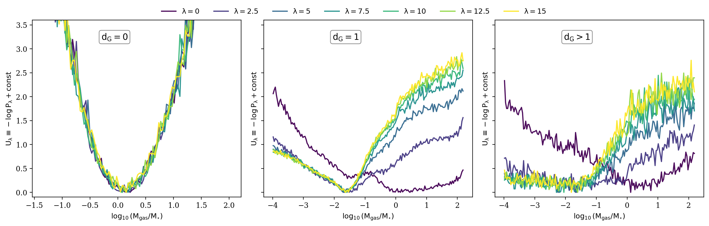
where $C_{\lambda,E}$ is an arbitrary additive constant, which we choose to normalize the minima to zero. The $U_{\lambda}(y\mid E)$ represents an effective potential that measures how typical or suppressed different values of $y$ are under the deformed trajectory distribution.

Figure 11 shows the projected log-probability profiles $U_{\lambda}$ distribution for the gas-to-stellar ratio in the three environment bins $d_{G}=0$, $d_{G}=1$, and $d_{G}>1$ from the left to right panels. The results demonstrate how the potentials of ratio histories are being reweighted by the deformation. First, the potential in the $d_{G}=0$ is nearly unchanged under the $\lambda$ deformation, which confirms that the environmental stripping does not operate on main halos. The minimum residing slightly above $y=0$ agrees with the fact that most of our $z=0$ main halos are gas-rich.

In the $d_{G}=1$ and $d_{G}>1$ bins (middle and right panels), increasing $\lambda$ drives the preferred endpoint ratio toward smaller $y=\log_{10}(M_{\rm gas}/M_{\star})$ and raises the cost of remaining at $y>0$, rendering gas-rich gas-rich galaxies less likely. This is precisely the signature expected if the host-edge gas channel mainly contributes to gas removal. Larger $\lambda$ suppresses trajectories that retain unusually large gas reservoirs relative to their stellar mass by $z=0$. Compared with the $d_{G}=1$ case, the $d_{G}>1$ potential becomes flatter at larger $\lambda$, particularly towards the lower $y$ region. This implies that the $d_{G}>1$ satellites still support a wider variety of histories, even as the gas-rich tail is progressively removed. The flattening in the $d_{G}>1$ effective potential matches the larger graph-to-graph scatter seen in Fig. 10.

The results presented in this section are fully consistent with our understanding of tidal stripping and ram-pressure stripping on gas depletion for satellites. They imply that environmental information carried by the host edges is successfully encoded in the learned residual dynamics of the GPLM.

VIII Path-Space Likelihood Diagnostics

The DMDG and gas-rich examples probe endpoint $z=0$ operators. They do not by themselves tell us how the host environment reshapes the ensemble of full satellite histories. This question can be addressed within GPLM because it assigns an explicit trajectory likelihood on each fixed layered graph. In this section, we introduce two path-space likelihood diagnostics to compare the full and host-ablated path measures. The results focus on the two satellite-node sets $E_{1}\equiv\{i:d_{G}(i)=1\}$ and $E_{>1}\equiv\{i:d_{G}(i)>1\}$. As in the previous examples, we sample full-graph trajectories jointly under the full kernel. For each dynamical term $(i,k)$, we then evaluate the log-likelihood of the realized increment under both the full and host-ablated Gaussian increment laws obtained from the same trained checkpoint, differing only in whether host edges are retained or removed.

This comparison naturally suggests a path-space perspective familiar from nonequilibrium stochastic thermodynamics. There, irreversibility is characterized by log-ratios between forward and backward path measures, whose mean defines an entropy-production-like cost and whose exponentiated form satisfies integral fluctuation identities when the reverse process is defined consistently. In the present coarse-grained galaxy setting, however, constructing a fully rigorous backward process remains nontrivial because node entry, infall events, and changing graph support introduce additional boundary structure. The diagnostics introduced below should therefore be viewed as preliminary path-space counterparts of such explorations. The statistic $W$ quantifies how strongly conditioning on host edges reshapes the forward-trajectory ensemble, while the local asymmetry proxy captures a more heuristic time-asymmetric signal in the learned increment law.

Figure 12: Left: graph-level intensive likelihood-ratio diagnostic $\bar{w}_{{\rm dyn},E}$, illustrated as violins for the test graphs in the $d_{G}=1$ and $d_{G}>1$ bins. The broader spread in the $d_{G}>1$ bins demonstrates that the host-edge has a more diverse effect in those satellites. Right: graph-level local asymmetry proxy $a_{{\rm dyn},E}^{(G)}$ for the same environment bins, shown for the full and host-ablated dynamics. The violins for the full-dynamics and host-edge-ablated cases are shaded in dark slate and brick red colors. As in the other examples, we use color code to display the graph ranks.

We first introduce a log likelihood-ratio diagnostic. Given two forward measures conditioned on the same graph $G$, $P_{\rm full}(\mathbf{x}\mid G)$ and $P_{\rm abl}(\mathbf{x}\mid G)$, define the trajectory log-likelihood ratio

$$W(\mathbf{x}\mid G)\equiv\log\frac{P_{\rm full}(\mathbf{x}\mid G)}{P_{\rm abl}(\mathbf{x}\mid G)}.$$ (41)

Sampling trajectories from $P_{\rm full}$ yields

$$\left\langle W\right\rangle_{P_{\rm full}}=D_{\rm KL}\left(P_{\rm full}|P_{\rm abl}\right)\geq 0,$$ (42)

so $W$ is an exact path-space diagnostic measuring the differences between the full and host-ablated dynamics. In the present setup, the comparison is carried out using the trajectory likelihood. The attachment enters identically in both cases and hence does not contribute to the contrast.

Here we report the $W$ averaged over the number of contributing terms and number of sampled trajectories, obtaining an intensive diagnostic

$$\bar{w}_{{\rm dyn},E}^{(G)}=\frac{1}{M_{G}}\sum_{m=1}^{M_{G}}w_{{\rm dyn},E}^{(m,G)},$$ (43)

where $M_{G}=512$ is the number of sampled trajectories per graph, $E\in\{E_{1},E_{>1}\}$ denotes the satellite-node set bin, and

$$w_{{\rm dyn},E}^{(m,G)}=\frac{W_{{\rm dyn},E}^{(m,G)}}{N_{{\rm dyn},E}^{(m,G)}}$$ (44)

is a number of contributions averaged per-trajectory intensive quantity, with $N_{{\rm dyn},E}$ being the number of dynamical increment terms in bin $E$, excluding newly attached nodes and counting the trained fields entering the trajectory likelihood. We also decompose $W$ into a quadratic residual term and a diffusion-volume term $(\log\det\Sigma)$, which allows us to test whether the environment acts mainly through drift alignment or through changes in the stochastic width.

The second diagnostic is a local asymmetry proxy, which is based on the same realized trajectories considering the increment log-likelihoods. We evaluate a forward and a reverse-proxy likelihood as

$$p_{i,k}^{\rm fwd}\equiv P_{\rm OM}(\Delta x_{i,k}\mid x_{i,k}),$$ (45)

$$p_{i,k}^{\rm rev,proxy}\equiv P_{\rm OM}(-\Delta x_{i,k}\mid x_{i,k}^{+}),$$ (46)

where the forward term evaluates the observed increment $\Delta x_{i,k}$ under the Gaussian increment law conditioned on the state $x_{i,k}$ before the step. The reverse-proxy term evaluates the sign-flipped increment $-\Delta x_{i,k}$ under the same kernel family, but conditioned on the endpoint state $x_{i,k}^{+}\equiv x_{i,k}+\Delta x_{i,k}$. The local asymmetry proxy is defined as

$$\Delta s_{{\rm dyn},i,k}^{\rm proxy}=\log\frac{p_{i,k}^{\rm fwd}}{p_{i,k}^{\rm rev,proxy}}.$$ (47)

It measures how differently the learned increment law treats the observed local step and its sign-flipped counterpart, serving as a local proxy for irreversibility through a forward-versus-reverse-proxy comparison.

At graph level we report

$$a_{{\rm dyn},E}^{{\rm proxy},(G)}=\frac{1}{M_{G}}\sum_{m=1}^{M_{G}}\left[\frac{1}{N_{{\rm dyn},E}^{(m,G)}}\sum_{(i,k)\in E}\Delta s_{{\rm dyn},i,k}^{\rm proxy,(m,G)}\right],$$ (48)

which uses the same two-step averaging as $\bar{w}_{{\rm dyn},E}^{(G)}$.

The left panel of Fig. 12 shows the path-space likelihood-ratio result $w_{{\rm dyn},E}$ in violins for the two environment bins. It shows that host-edge conditioning changes the full trajectory ensemble in both bins, with the $d_{G}>1$ case displaying a broader distribution and a slightly higher median. It means the host-edge has a more diverse effect on the $d_{G}>1$ satellites, but on average, the effects are close when measured at the median. Decomposing the $w_{\rm dyn}$ into quadratic residual terms and diffusion-volume terms, we obtain

$${\rm med}\left[w^{\rm quad}_{d_{G}=1}\right] \simeq 93,\quad{\rm med}\left[w^{\rm quad}_{d_{G}>1}\right]\simeq 33,$$ (49)

$${\rm med}\left[w^{\log\det}_{d_{G}=1}\right] \simeq-40,\quad{\rm med}\left[w^{\log\det}_{d_{G}>1}\right]\simeq-43,$$

where the quadratic residual terms dominate the $w_{\rm dyn}$ values. This implies that host-edge conditioning changes the predicted mean evolution far more than it changes the predicted covariance. It also tells us that GPLM encodes environmental effects that reorganize the mean direction of satellite evolution rather than merely broadening the stochastic width.

The right panel of Fig. 12 shows the violins for the local asymmetry proxy $a_{{\rm dyn},E}$ in both the full-dynamics and host-edge-ablated cases. We observe that the full-dynamics violins have lower medians but broader spreads than the host-ablated violins. This suggests that host-edge conditioning improves local alignment on average, while also introducing additional graph-dependent structure into the trajectory ensemble, thereby increasing the scatter. This broader spread likely reflects the greater diversity of environmental histories encoded by the host-edge conditioning.

The two diagnostics in this section separate two complementary questions. The statistic $w_{\rm dyn}$ measures how strongly host-edge conditioning changes the full trajectory ensemble, while $a_{\rm dyn}^{\rm proxy}$ tracks how host-edge conditioning modifies the local time-asymmetric structure of the learned increment law. These examples show that the graph-conditioned likelihood can be used to compare entire classes of histories in path space. Pursuing this direction could support graph-conditioned typicality studies, rare-path analyses, and a more refined separation of merger-driven and environment-driven dynamical effects within the same probabilistic framework Seifert (2012); Chetrite and Gawȩdzki (2008); Crooks (1999); Jarzynski (1997).

IX Discussion and Conclusions

This work formulates galaxy formation as a graph-conditioned trajectory ensemble with an explicit path measure. On a fixed layered halo graph $G$, GPLM assigns the baryonic history $\mathbf{x}$ the conditional weight

$$P(\mathbf{x}\mid G)\propto p_{\rm attach}(\mathbf{x}\mid G)\exp[-S_{\rm OM}(\mathbf{x}\mid G)],$$ (50)

which extends to the joint measure $P(\mathbf{x},G)=P(\mathbf{x}\mid G)P(G)$ once a graph-sector model is specified. As a concrete implementation, a graph-based neural network model is trained to predict residual drifts with diffusion on top of deterministic merger transport. The likelihood is written as a functional of baryonic trajectories through an effective action, currently implemented with a Gaussian OM term. This path-space formulation enables graph-conditioned operator averages, controlled response deformations, and related diagnostics to be computed within a single normalized probabilistic framework. Organizing inference at the trajectory level in this way makes GPLM conceptually distinct from summary-level forward models, field reconstructions, and graph-based emulators.

IX.1 Applications to Dark Matter Microphysics

The likelihood formulation on layered halo graphs naturally connects to dark matter microphysics, such as self-interacting dark matter (SIDM). A direct continuation is an SIDM version of GPLM inspired by the parametric model developed in Yang et al. (2024, 2025a); Yang (2024). In that model, an integral approach applies a universal analytic kernel incrementally on a halo’s $V_{\max}$ and $R_{\max}$ evolution history in cold dark matter, mapping the evolution trajectories into SIDM, incorporating the effect of gravothermal evolution along with the accretion history. These features naturally fit into the GPLM framework. The $V_{\max}$ and $R_{\max}$ are fields that evolve along merger histories, and a trained GNN model that works incrementally in a time-universal manner mirrors the analytic kernel. For an increment at a specific layer, one can write schematically

$$\Delta\mathbf{y}_{k}=\Delta\mathbf{y}^{\rm tr}_{k}+\Delta\tau_{k}\,\mathbf{b}_{\rm SIDM}(s_{k};\theta)+\boldsymbol{\epsilon}_{k},$$ (51)

with $\mathbf{y}_{k}\equiv(V_{\max},R_{\max})_{k}$ and $\mathbf{y}^{\rm tr}_{k}$ a nonlinear transport map to propagate the two structural variables. Here $\mathbf{b}_{\rm SIDM}$ represents a residual drift in the spirit of the integral approach, while $\boldsymbol{\epsilon}_{k}$ captures residual scatter from limited conditioning and unresolved physics. The conditioning on local graph state, transported fields, redshift, etc., enables the proposed framework to capture the environmental stripping effect and improve upon human-calibrated analytic kernels. Depending on details of the unresolved variability, one may even augment the model to incorporate non-Gaussian terms. The path-action based formulation also facilitates simultaneous exploration of the baryonic and dark matter contents. Models beyond elastic SIDM, such as dissipative SIDM and two-component SIDM with mass segregation, exhibit analogous developments and can thus be explored within the same formalism Yang et al. (2025b); Essig et al. (2019).

IX.2 Toward a Full Multi-Field Galaxy-Formation Theory

A natural next step is to extend GPLM from the present two-field example to a multi-field theory of galaxy formation on layered graphs. Relevant variables can include gas and star half-mass radii, star-formation activity, metallicity, black-hole mass, and halo structural properties, etc. The graph construction and deterministic transport bookkeeping could be the same, but the residual sector will become multivariate, graph-local couplings could be introduced, and higher-order corrections could be added systematically. Meanwhile, as mentioned for SIDM, non-linear maps could be included to transport fields other than masses.

Another possible extension is a joint history action,

$$S_{\rm tot}=S_{G}[G_{0:K}]+S_{x}[\mathbf{x}_{0:K};G_{0:K}]+S_{\rm bnd}[\mathbf{x}_{0:K};G_{0:K}],$$ (52)

with

$$P(G_{0:K})\propto\exp\left[-\sum_{k}S_{G,k}\right],$$ (53)

where $S_{x}$ is the conditional field action on that history, $S_{\rm bnd}$ is a boundary action associated with node entry, and $S_{G}$ is an action that governs graph-construction. This formulation provides a route to a fully generative theory of graph and field histories.

The current GNN-based construction could also be extended by incorporating semi-analytic model predictions into the increments. Such an approach would allow existing physical knowledge to serve as an analytic backbone while GPLM captures the remaining unresolved structure and its associated scatter. In this setting, future refinements may be evaluated not only by predictive accuracy but also by whether they help identify a useful operator basis. Ideally, such a basis would remain both expressive and interpretable. In practice, this could involve separating transport, environmental, boundary, and higher-order non-Gaussian contributions, while assessing case by case whether cross-field couplings should remain implicit through conditioning or be promoted to explicit operators for improved interpretability and response control.

The conceptual perspective of this work can be stated simply. Galaxy formation is formulated here as a graph-conditioned path ensemble with an associated effective action, enabling the description of probabilities, rare-event statistics, and response diagnostics within a common probabilistic framework. In this sense, GPLM goes beyond a purely conditional emulator and provides a common language for layered assembly graphs, stochastic galaxy trajectories, and path-space diagnostics, while remaining open to richer graph histories, broader operator bases, and more refined microphysical applications in future work.

The training and testing codes used in this work are available at: https://github.com/DanengYang/GraphPathLikelihood

Appendix A Layers of spatial halo graphs

To visualize the layered construction, we show the host-edge subgraphs obtained by removing temporal edges from the rank-1 layered halo graph. Figures 13 and 14 illustrate these graphs at layers corresponding to redshifts from $3$ to $0$, in a topological view (spring layout) and a physical view (comoving coordinates), respectively. In the topological view, the system initially contains many isolated small graphs, most of them containing only one node. They merge into larger graphs and eventually form a single graph at $z=0$. In physical coordinates, their spatial clustering is more clearly displayed, with nodes gathering over time and moving into the virial radius of the endpoint ($z=0$) host halo. In all the panels, edges encode coeval host-satellite assignments that link satellites to their least-massive enclosing host halo Yang and Yu (2023).

Figure 13: Topological (spring-layout) view of the host-edge subgraphs for the rank-1 layered halo graph at multiple snapshots obtained by removing temporal edges. From top-left to bottom-right the panels correspond to increasing redshift: $z=0,0.1,0.2,0.3,0.4,0.5,0.7,1,1.5,2$. Only the $z=3$ snapshot is left over due to limited space.

Figure 14: Physical (comoving-coordinate) view of the same host–edge subgraphs shown in Fig. 13. The snapshot ordering follows the topological view: $z=0,0.1,0.2,0.3,0.4,0.5,0.7,1,1.5,$ and $2$. The $z=3$ snapshot is omitted due to space limitations. This presentation enables a direct comparison between the graph connectivity and the corresponding spatial configuration at the same cosmic time.

Appendix B Attachment Fits for Newly Included Nodes

The attachment factor $p_{\rm attach}$ supplies the boundary part of the graph-conditioned likelihood. Once a node is already linked to the layered graph by a temporal edge, its subsequent evolution is governed by the GPLM trajectory likelihood. By contrast, when a node first appears in the constructed graph without a progenitor in the adjacent earlier layer, its initial $(M_{\star},M_{\rm gas})$ values must be specified separately. In the present implementation, that boundary sector is modeled through the approximate factorization

$$p_{\rm attach}\approx P(M_{\star}\mid M_{\rm halo},z)\,P(M_{\rm gas}\mid M_{\rm halo},z),$$ (54)

which provides a pragmatic closure for entry into the graph while leaving the in-graph environmental evolution to the learned trajectory measure.

The sample used for this fit should be interpreted in the same effective sense as the graph construction itself. Our layered halo graphs are designed to retain the halos most relevant to the $z=0$ host and to connect them through temporal and host edges. However, due to technical and resolution limitations, they do not form a fully closed merger forest in every case. In particular, temporal links are only added between adjacent retained layers when a progenitor passing the mass threshold is identified. With the relatively sparse layer spacing used here, some halos could grow substantially between two retained layers and enter the constructed graph without incoming temporal edges from the previous layer. In the massive cases, their entries come together with the coeval host-edge structure, with the associated lower-mass nodes entering simultaneously. As a result, the attachment sample contains a spectrum of boundary nodes, from isolated low-mass entries to host-connected systems that appear after rapid growth between the retained layers.

Additional missing temporal edges can also arise from limitations of the merger construction itself. In particular, temporary irregularities in the SubLink histories can introduce spurious boundary nodes and blur the intended separation between the $p_{\rm attach}$ sector and the interior trajectory likelihood. In practice, this mainly widens the effective scatter in $p_{\rm attach}$. The GPLM dynamics is trained on simulation data embedded in the constructed graphs, and its accuracy is less affected.

The calibration is carried out on all constructed graphs using nodes with no incoming temporal edge from the previous retained layer, together with a halo-mass cut $M_{\rm halo}>10^{8}~\rm M_{\odot}/h$ and a mass-weighting scheme that reduces the dominance of the most numerous low-mass points. Table 1 summarizes the number of entering nodes in each retained layer. The boundary sector is concentrated in the early retained snapshots. Out of 21,319 entering nodes in the full calibration sample, about 54% appear by snapshot 50 and about 65% by snapshot 59. This pattern indicates that $p_{\rm attach}$ mainly controls early-time entry into the constructed layered graphs, while its influence becomes progressively smaller at later times.

Table 1: Number of entering nodes used in the $p_{\rm attach}$ calibration at each retained snapshot. Here $N_{\rm new}$ is the number of nodes with no incoming temporal edge from the previous retained layer, $N_{\rm layer}$ is the total number of nodes in that layer, and $f_{\rm new}\equiv N_{\rm new}/N_{\rm layer}$.

Snapshot	$N_{\rm new}$	$N_{\rm layer}$	$f_{\rm new}$
17	444	444	1.000
21	685	1118	0.613
25	1309	2324	0.563
33	3440	5381	0.639
40	2590	6730	0.385
50	3126	8066	0.388
59	2205	8252	0.267
67	1879	8121	0.231
72	1437	7804	0.184
78	1555	7515	0.207
84	1438	6954	0.207
91	810	5746	0.141
99	401	4017	0.100

The attachment model is defined in log space as a two-branch linear relation,

$$y_{\rm lo}(x)=\alpha_{\rm lo}+\beta_{\rm lo}x,\qquad y_{\rm hi}(x)=\alpha_{\rm hi}+\beta_{\rm hi}x,$$ (55)

where $x\equiv\log_{10}[M_{\rm halo}/(10^{10}M_{\odot}/h)]$ and $y\equiv\log_{10}[M_{\star}/(10^{10}M_{\odot}/h)]$ or $y\equiv\log_{10}[M_{\rm gas}/(10^{10}M_{\odot}/h)]$. To avoid a discontinuity at the transition, we blend the two branches smoothly,

$$w(x)=\frac{1}{1+\exp\left[-(x-x_{\rm split})/\Delta\right]},\qquad\mu(x)=[1-w(x)]y_{\rm lo}(x)+w(x)y_{\rm hi}(x),$$ (56)

using $x_{\rm split}=0.4$ for $M_{\star}$ and $x_{\rm split}=0.5$ for $M_{\rm gas}$, with $\Delta=0.2$ in the fiducial setup. We then model the conditional distribution as a lognormal (Gaussian in $y$) with mean $\mu(x)$ and scatter $\sigma(x)$. In the two-branch case, the scatter is blended in the same way,

$$\sigma(x)=[1-w(x)]\sigma_{\rm low}+w(x)\sigma_{\rm high},$$ (57)

where $\sigma_{\rm low}$ and $\sigma_{\rm high}$ are estimated from the weighted residuals in the low- and high-mass branches, respectively. Improved layered-graph construction with finer retained timesteps and more complete merger-history tracking should lead to a cleaner boundary sector and a more robust graph-path likelihood in future work.