Transformers As Generalizable Optimal Controllers

Abstract

We study whether optimal state-feedback laws for a family of heterogeneous Multiple-Input, Multiple-Output (MIMO) Linear Time-Invariant (LTI) systems can be captured by a single learned controller. We train one transformer policy on LQR-generated trajectories from systems with different state and input dimensions, using a shared representation with standardization, padding, dimension encoding, and masked loss. The policy maps recent state history to control actions without requiring plant matrices at inference time. Across a broad set of systems, it achieves empirically small sub-optimality relative to Linear Quadratic Regulator (LQR), remains stabilizing under moderate parameter perturbations, and benefits from lightweight fine-tuning on unseen systems. These results support transformer policies as practical approximators of near-optimal feedback laws over structured linear-system families.

I Introduction

Transformers are now widely used for learning from sequences. This motivates their use in feedback control settings where recent history can carry information about the underlying dynamics. This paper addresses the following question: Can one transformer policy be trained to produce near-optimal feedback actions across a family of linear models? This is motivated by robotics and cyber-physical systems, where the models can change over time due to operating-point shifts, payload changes, contact conditions, temperature effects, wear, or online re-identification. In these cases, the controller must adapt quickly and repeatedly, sometimes under limited computation or limited new data.

The paper proposes a unified learning framework that casts optimal control into a sequence-to-control problem across heterogeneous systems. Specifically, we consider the discrete-time LQR problem [1]. The method builds a training set by simulating the optimal state feedback controllers on many model variants and many initial conditions. Then, a multi-block transformer policy is trained on these samples and can be deployed to produce a control action.

The contributions of this paper are threefold. First, we formulate cross-system LQR imitation as a sequence-to-control problem over heterogeneous LTI systems. Second, we introduce a shared representation and masking scheme that lets one policy train across different state and input dimensions. Finally, we show empirical near-optimality and robustness over a broad family of perturbed systems, and rapid few-shot adaptation on unseen systems.

II Related Work

II-A Optimal and robust control

LQR is a classical optimal control problem. The optimal state feedback for LTI systems can be constructed from the solution of an algebraic Riccati equation [1]. Robust control and gain scheduling extend these ideas to handle uncertainty and parameter variation, using $\mathcal{H}_{\infty}$, $\mu$-synthesis or linear parameter-varying (LPV) formulations to guarantee performance over bounded perturbations [19, 14]. These methods yield per-system controllers tailored to a given plant or uncertainty description, but do not construct a single parametric policy that is nearly optimal across an entire collection of systems.

II-B Neural and generalist control policies

Neural networks have long been used to approximate feedback laws and adaptive controllers, including early work on neural control of robot manipulators and nonlinear systems [10]. In reinforcement learning, generalizable policies are trained to operate across a distribution of models and adapt via online system identification or dynamics randomization [18, 13]. More recently, large multi-robot datasets have enabled generalist and cross-embodiment policies such as RT-1 for real-world manipulation [2], Open X-Embodiment and RT-X [11], Octo [12], and CrossFormer, which controls manipulators, mobile robots, quadrupeds, and aerial vehicles with a single transformer backbone [5]. Foundation-style models are also emerging at the level of low-level dynamics: AnyCar learns a transformer-based universal dynamics model for agile wheeled robots [17], while RAPTOR trains a compact recurrent foundation policy that enables zero-shot adaptation to diverse quadrotors [7]. These works demonstrate strong empirical generalization across platforms and tasks, but do not construct a single policy trained from optimal control supervision to control a diverse group of dynamical systems.

II-C Transformers for dynamics, control, and LLMs

Transformers were introduced for sequence modeling in natural language [15], with architectural choices such as GELU activations [9] and large-scale evaluation methodologies [3] underpinning modern LLMs. Beyond language, transformers have been used to learn surrogate models of physical and dynamical systems [8], to approximate optimal filters for unknown systems [6], and to accelerate trajectory optimization and model predictive control (MPC), for example by parallelizing iLQR updates [16] or casting control as sequence modeling in the Decision Transformer [4]. In all of these cases, transformers are employed as function approximators for specific tasks or individual systems. In contrast, this work analyzes a structured family of linear systems and associated LQR problems, and shows that a single transformer is a generalizable near-optimal controller.

III Problem Formulation

Consider the following LTI system:

$$x_{t+1}=Ax_{t}+Bu_{t},$$ (1)

where $x_{t}\in\mathbb{R}^{n}$ and $u_{t}\in\mathbb{R}^{m}$ are the state and input at time $t$, respectively. We assume the full state is measurable and aim to design a state feedback policy $u_{t}=\pi(x_{t})$. Starting from an initial state $x_{0}$, the goal is to stabilize the plant and minimize the following infinite-horizon quadratic performance index:

$$\mathcal{J}(x_{0};\pi):=\sum_{t=0}^{\infty}x_{t}^{\top}Qx_{t}+u_{t}^{\top}Ru_{t},$$ (2)

where $Q\succeq 0$ and $R\succ 0$. We further assume: (i) $(A,B)$ is stabilizable and (ii) $(Q^{1/2},A)$ is detectable. This corresponds to the infinite-horizon, discrete-time Linear Quadratic Regulator (LQR) problem [1]. Assumptions (i) and (ii) are standard to ensure the problem is well-posed.

The solution for this optimization problem is known to be $u_{t}^{\star}=\pi^{\star}(x_{t})=-K^{\star}x_{t}$ with

$$K^{\star}=\bigl(R+B^{\top}PB\bigr)^{-1}B^{\top}PA,$$ (3)

where $P$ satisfies the Algebraic Riccati Equation (ARE)

$$P=Q+A^{\top}PA-A^{\top}PB\bigl(R+B^{\top}PB\bigr)^{-1}B^{\top}PA.$$ (4)

The optimal cost is given by $\mathcal{J}(x_{0};\pi^{\star})=x_{0}^{\top}Px_{0}$.

Our goal is to use transformers to learn a single state-feedback policy for a collection of systems. Specifically, assume we are given problem data for a set of LQR problems, denoted $\{A^{(i)},B^{(i)},Q^{(i)},R^{(i)}\}_{i=1}^{N}$. Each problem instance can have different state and input dimensions, denoted $(n_{x}^{(i)},n_{u}^{(i)})$ for $i=1,2,\ldots,N$. In addition let $\pi^{\star,(i)}$ denote the optimal controller for problem $i$.

We seek to design a single universal parameterized policy that is stabilizing and produces a nearly optimal quadratic cost for each specific system. The universal policy is a state feedback controller that has the form $\pi_{\phi}\left(\{x_{l}\}_{l=t-w}^{t},n_{x},n_{u}\right)$ where $\phi\in\mathbb{R}^{k}$ is a vector of parameters that define the policy and $\{x_{l}\}_{l=t-w}^{t}$ is a sequence of states from time $t-w$ to $t$. The universal state feedback policy is static but uses the current and past $w$ state measurements. Here, $w\in\mathbb{N}$ defines the window length and $(n_{x},n_{u})$ defines the problem dimensions. We attempt to learn a single policy parameter vector $\phi$ to minimize the sub-optimality over $N$ problem instances with $J$ different initial conditions for each problem:

$$\operatorname*{arg\,min}_{\phi}\ \sum_{i=1}^{N}\sum_{j=1}^{J}\left[\mathcal{J}^{(i)}\big(x_{0}^{(i,j)};\pi_{\phi})-\mathcal{J}^{(i)}(x_{0}^{(i,j)},\pi^{\star,(i)})\right],$$ (5)

where $\mathcal{J}^{(i)}$ is the LQR cost function for problem $i$ as defined by $Q^{(i)}$ and $R^{(i)}$. Expression (5) yields a $\phi^{\star}$ that defines our single universal policy $\pi_{\phi^{\star}}$. This universal policy provides a reasonably good controller for many systems. Moreover, $\phi^{\star}$ can also be used as an initializer to fine-tune the policy parameter for unseen systems with minimal retraining.

IV Approach

This section describes our proposed method for using transformers to learn a single universal control policy, $u_{t}=\pi_{\phi}\left(\{x_{l}\}_{l=t-w}^{t},n_{x},n_{u}\right)$. This is implemented with three steps. First, a system-wise standardization is used to map the data $(u_{t},\{x_{l}\}_{l=t-w}^{t},n_{x},n_{u})$ to a standard form $(\bar{u}_{t},S_{t})$ (Section IV-B). Next, a transformer is used to realize a policy $\bar{\pi}_{\phi}$ that maps the standard input $S_{t}$ to the standard control $\bar{u}_{t}$ (Section IV-C). Finally, the standard control $\bar{u}_{t}$ is mapped back to the actual control $u_{t}$ (Section IV-D). This section describes these three steps in detail. It also presents the transformer design, training for generalizable optimal control, and fine-tuning for unseen systems.

IV-A Data Collection

Let $\mathcal{S}^{(i)}=(A^{(i)},B^{(i)},Q^{(i)},R^{(i)})$ denote the plant and cost matrices for one LQR problem $i\in\{1,\ldots,N\}$. We simulate this problem instance with the optimal LQR state feedback $\pi^{\star,(i)}(x_{t})=-K^{\star,(i)}x_{t}$ from $J$ different initial conditions $x_{0}^{(i,j)}$ with $j=1,\ldots,J$. This yields $J$ different state and control sequences: $X^{(i,j)}=\{x_{0}^{(i,j)},\cdots,x_{T-1}^{(i,j)}\}$ and $U^{(i,j)}=\{u_{0}^{(i,j)},\cdots,u_{T-1}^{(i,j)}\}$. The combined data set for the $i$th problem then consists of $X^{(i)}:=\{X^{(i,j)}\}_{j=1}^{J}$ and $U^{(i)}:=\{U^{(i,j)}\}_{j=1}^{J}$. We repeat this process for each problem instance $i=1,\ldots,N$. Finally, the combined state and control dataset is $\{(X^{(i)},U^{(i)})\}_{i=1}^{N}$.

The $N$ different problem instances and the trajectories are generated in a way that ensures enough coverage and diversity to enrich the learning process. To do so, we pick a group of LTI systems that includes mechanical, electrical, and robotic systems. After that, each individual system’s parameters are varied to form a collection of variant systems per individual LTI system. Thus, each variant has its unique index $i$ in the set of systems we consider. Furthermore, the trajectories of each model $i$ are generated from numerous random initial conditions within a predefined bound.

IV-B Data Processing

The main objective is to recast system-specific LQR supervision into a common sequence-to-action learning problem, while preserving sufficient information for the model to adapt its predictions to each system structure. The data processing consists of sequence preparation and dimension encoding.

The first step of the sequence preparation is to perform system-wise standardization. This normalization addresses scale differences across various systems. Consider the state and input data $(X^{(i)},U^{(i)})$ associated with problem $i\in\{1,\ldots,N\}$. This data set includes $J$ different state and control sequences. To simplify the notation, we will temporarily drop the superscript $i$ for the specific problem and only denote the trajectory index $j$, e.g., $x_{t}^{(i,j)}$ is simplified to $x_{t}^{(j)}$ to denote a state for any system with initial condition $j$ at time step $t$. Let $1_{n_{x}}\in\mathbb{R}^{n_{x}}$ be a vector with all entries equal to one. Define the sample mean and standard deviation of the state-sequence data for problem $i$ by the following scalars:

$$\mu_{x} :=\frac{1}{JTn_{x}}\sum_{j=1}^{J}\sum_{t=0}^{T-1}\left(1_{n_{x}}^{T}\,x_{t}^{(j)}\right),$$ (6)

$$\sigma_{x} :=\left(\frac{1}{JT-1}\sum_{j=1}^{J}\sum_{t=0}^{T-1}\left\|x_{t}^{(j)}-\mu_{x}1_{n_{x}}\right\|^{2}\right)^{1/2}.$$ (7)

The state mean and standard deviation are computed separately for each $i\in\{1,\ldots,N\}$. The mean and standard deviation for the input-sequence data of problem $i$, denoted $\mu_{u}$ and $\sigma_{u}$, are defined similarly.

We use these problem-specific statistics to normalize the trajectories. Specifically, consider the $j$th trajectory for problem $i$. We transform each element of these trajectories as follows

$$\hat{x}_{t}^{(j)}=\frac{x_{t}^{(j)}-\mu_{x}1_{n_{x}}}{\sigma_{x}},\qquad\hat{u}_{t}^{(j)}=\frac{u_{t}^{(j)}-\mu_{u}1_{n_{u}}}{\sigma_{u}}.$$ (8)

This normalization maps all training samples into a shared representation space. This enables stable optimization and effective learning across systems. During inference, predicted controls are de-standardized using the same system-specific statistics to recover physically meaningful actions.

Next, the systems may have different state and control dimensions. We use zero-padding to unify input and output dimensions. Specifically, let Pad$(\hat{x}_{t},n_{x}^{\mathrm{max}})$ denote the $n_{x}^{\mathrm{max}}\times 1$ vector obtained by padding $(n_{x}^{\mathrm{max}}-n_{x})$ zero entries to the vector $\hat{x}_{t}\in\mathbb{R}^{n_{x}}$. We use this zero-padding to map the normalized state and control data to a standard, maximum dimension:

$$\bar{x}_{t}^{(j)}=\mathrm{Pad}\big(\hat{x}_{t}^{(j)},\,n_{x}^{\mathrm{max}}\big),\quad\bar{u}_{t}^{(j)}=\mathrm{Pad}\big(\hat{u}_{t}^{(j)},\,n_{u}^{\mathrm{max}}\big).$$ (9)

The transformer takes fixed-length sequences of normalized, zero-padded data over a sliding window of length $w$, allowing recent history to serve as an implicit form of system identification. For each starting time $t$, the standardized state sequence is $\{\bar{x}_{t-w}^{(j)},\bar{x}_{t-w+1}^{(j)}\ldots,\bar{x}_{t}^{(j)}\}$. This corresponds to a stride length of one, but stride lengths greater than one could be used. The learning target is the next control $\bar{u}_{t}$.

We construct a binary dimension encoding vector to explicitly inform the transformer about the active state and control dimensions of the specific problem. Let $\mathrm{Binary}(n_{x})$ denote the row vector of the binary representation for the state dimension $n_{x}$ for problem $i$. This requires $d_{x}=\left\lceil\log_{2}(n_{x}^{\mathrm{max}})\right\rceil$ bits. Similarly, $\mathrm{Binary}(n_{u})$ is a binary representation for the input dimension $n_{u}$ of problem $i$ with $d_{u}=\left\lceil\log_{2}(n_{u}^{\mathrm{max}})\right\rceil$ bits. This encoding is appended to the zero-padded state vector at every time step, yielding the transformer input sequence at time $t$:

$$S_{t}^{(j)}=\begin{bmatrix}(\bar{x}_{t-w}^{(j)})^{T}\oplus\mathrm{Binary}(n_{x})\oplus\mathrm{Binary}(n_{u})\\ \vdots\\ (\bar{x}_{t}^{(j)})^{T}\oplus\mathrm{Binary}(n_{x})\oplus\mathrm{Binary}(n_{u})\end{bmatrix}.$$ (10)

The transformer input, for any problem instance, has a standard dimension $(w+1)\times d_{\mathrm{in}}$ with the column dimension $d_{\mathrm{in}}=n_{x}^{\mathrm{max}}+d_{x}+d_{u}$.

Finally, we define a binary control mask to prevent the model from being penalized on padded control dimensions. Let $1_{n_{u}}$ be the $n_{u}$ vector with all entries equal to one. The binary mask for problem $i$ is $\kappa:=\mathrm{Pad}\big(1_{n_{u}},\,n_{u}^{\mathrm{max}}\big)$. This vector has $n_{u}$ ones stacked above $n_{u}^{\mathrm{max}}-n_{u}$ zeros. Each training sample is stored as the triplet $(S_{t}^{(j)},\bar{u}_{t}^{(j)},\kappa)$. The complete dataset $\mathcal{D}$ consists of all training samples formed from each time $t\in\{0,\ldots,T\}$ for all trajectories $j\in\{1,\ldots,J\}$ of each problem $i\in\{1,\ldots,N\}$.

IV-C Transformers

Attention transformers [15] are the state-of-the-art neural models in learning complex temporal patterns, especially in Large Language Models [3]. This section first describes the single-transformer neural model. The extension to a multi-transformer neural model is then discussed.

First, we introduce the design of a single transformer block. Consider the sequence $S_{t}$ as defined in (10), where we drop the superscript $j$ for simplicity. The transformer realizes a policy on this standardized data, $\bar{\pi}_{\phi}:\mathbb{R}^{(w+1)\times d_{\mathrm{in}}}\to\mathbb{R}^{n_{u}^{max}}$, with parameters $\phi$. This policy takes the input data $S_{t}$ at time $t$ and generates the standardized control $\bar{u}_{t}=\bar{\pi}_{\phi}(S_{t})$. The mapping from this standardized control $\bar{u}_{t}\in\mathbb{R}^{n_{u}^{\mathrm{max}}}$ back to the actual control $u_{t}\in\mathbb{R}^{n_{u}}$ is discussed later.

The first transformer operation embeds the sequence into width $d_{\mathrm{m}}$ by a time-wise affine map applied in matrix form,

$$\mathcal{Z}=S_{t}W_{\mathrm{in}}^{\top}+1_{w+1}b_{\mathrm{in}}^{\top}\ \in\ \mathbb{R}^{(w+1)\times d_{\mathrm{m}}},$$ (11)

where $W_{\mathrm{in}}\in\mathbb{R}^{d_{\mathrm{m}}\times d_{\mathrm{in}}}$, and $b_{\mathrm{in}}\in\mathbb{R}^{d_{\mathrm{m}}}$. A learned positional matrix $\mathcal{P}\in\mathbb{R}^{(w+1)\times d_{\mathrm{m}}}$ is then added to encode temporal order,

$$H=\mathcal{Z}+\mathcal{P}\ \in\ \mathbb{R}^{(w+1)\times d_{\mathrm{m}}}.$$ (12)

Fix a head index $i\in\{1,\dots,h\}$ with head width $d_{h}$ satisfying $d_{\mathrm{m}}=hd_{h}$. The per-head query, key, and value matrices are obtained from $H$ by linear projections,

$$\mathcal{Q}^{(i)}=HW_{\mathcal{Q}}^{(i)},\quad\mathcal{K}^{(i)}=HW_{\mathcal{K}}^{(i)},\quad\mathcal{V}^{(i)}=HW_{\mathcal{V}}^{(i)},$$ (13)

where $W_{\mathcal{Q}}^{(i)},W_{\mathcal{K}}^{(i)},W_{\mathcal{V}}^{(i)}\in\mathbb{R}^{d_{\mathrm{m}}\times d_{h}}$ and $\mathcal{Q}^{(i)},\mathcal{K}^{(i)},\mathcal{V}^{(i)}\in\mathbb{R}^{(w+1)\times d_{h}}$. The head-$i$ attention logits are assembled as a full matrix, $\mathbb{L}^{(i)}=\frac{\mathcal{Q}^{(i)}(\mathcal{K}^{(i)})^{\top}}{\sqrt{d_{h}}}\ \in\ \mathbb{R}^{(w+1)\times(w+1)}$. The corresponding attention weights are obtained by applying softmax row-wise as $\mathcal{A}^{(i)}=\texttt{softmax}\big(\mathbb{L}^{(i)}\big)\ \in\ \mathbb{R}^{(w+1)\times(w+1)}$. A single matrix multiplication computes the head-$i$ context as $H^{(i)}=\mathcal{A}^{(i)}\mathcal{V}^{(i)}\ \in\ \mathbb{R}^{(w+1)\times d_{h}}$, which aggregates values according to the attention weights. Having formed $H^{(i)}$ for all heads, the multi-head output is assembled by concatenation followed by an output projection,

$$H^{\mathrm{cat}} =\big[H^{(1)},\cdots,H^{(h)}\big]\ \in\mathbb{R}^{(w+1)\times d_{m}},$$ (14)

$$\mathcal{A} =H^{\mathrm{cat}}W_{O}\in\mathbb{R}^{(w+1)\times d_{\mathrm{m}}},$$ (15)

with $W_{O}\in\mathbb{R}^{d_{m}\times d_{\mathrm{m}}}$.

Next, we define the normalization layer $\texttt{LN}(x)$ as follows. Denote the mean and variance for a vector $x\in\mathbb{R}^{d}$ by $\mu(x)$ and $\sigma^{2}(x)$. The layer normalization recenters and rescales $x$ and applies an affine transform:

$$\texttt{LN}(x)\;=\;\gamma\odot\frac{x-\mu(x)1_{d}}{\sqrt{\sigma^{2}(x)+\rho}}+\beta,$$ (16)

where $\gamma,\beta\in\mathbb{R}^{d}$ are learnable parameters. Here $\odot$ denotes element-wise multiplication, and $\rho$ is a small constant for numerical stability. $\texttt{LN}(\cdot)$ can also operate on a matrix by operating on its rows.

Residual addition and layer normalization stabilize the feature scale as follows

$$\mathcal{C}=\texttt{LN}\big(H+\mathcal{A}\big)\in\mathbb{R}^{(w+1)\times d_{\mathrm{m}}}.$$ (17)

This is then passed through a position-wise feed-forward mapping written in matrix form,

$$F =\texttt{GELU}\big(\mathcal{C}W_{1}+1_{w+1}b_{1}^{\top}\big)\ \in\ \mathbb{R}^{(w+1)\times d_{\mathrm{ff}}},$$ (18)

$$G =FW_{2}+1_{w+1}b_{2}^{\top}\in\mathbb{R}^{(w+1)\times d_{\mathrm{m}}},$$ (19)

where $W_{1}\in\mathbb{R}^{d_{\mathrm{m}}\times d_{\mathrm{ff}}}$, $W_{2}\in\mathbb{R}^{d_{\mathrm{ff}}\times d_{\mathrm{m}}}$, $b_{1}\in\mathbb{R}^{d_{\mathrm{ff}}}$, $b_{2}\in\mathbb{R}^{d_{\mathrm{m}}}$. GELU [9] is the activation applied element-wise, and $d_{\mathrm{ff}}$ is a design hyperparameter.

After computing (19), the single-transformer block output is obtained by a second residual addition and normalization,

$$Y=\texttt{LN}\big(\mathcal{C}+G\big)\ \in\ \mathbb{R}^{(w+1)\times d_{\mathrm{m}}}.$$ (20)

This concludes the single transformer block design. The function $\mathrm{Block}\big(H\big)$ describes this process (i.e., (12) to (20)).

Next, we form a multi-transformer-block design. Starting from the single-block output $Y\in\mathbb{R}^{(w+1)\times d_{\mathrm{m}}}$, the control can be produced from multiple transformer blocks by aggregating the last-time representations from each block. Let $L\in\mathbb{N}$ denote the number of blocks. For each $\ell=1,\dots,L$, apply one transformer block to the hidden sequence $H$ to obtain $Y^{(\ell)}=\mathrm{Block}_{\ell}\big(H\big)\in\mathbb{R}^{(w+1)\times d_{\mathrm{m}}}$, where $Y^{(\ell)}\in\mathbb{R}^{(w+1)\times d_{\mathrm{m}}}$. We extract the last row from each block output $Y^{(\ell)}$ and convert it to a column vector $r^{(\ell)}=\left(Y^{(\ell)}(w+1,:)\right)^{T}\in\mathbb{R}^{d_{\mathrm{m}}}$. Then, these vectors are stacked by feature-wise concatenation to form the layer-aggregated feature,

$$\mathcal{R}=\big[r^{(1)};r^{(2)};\dots;r^{(L)}\big]\in\mathbb{R}^{Ld_{\mathrm{m}}}.$$ (21)

The aggregated feature is then mapped to the control space by a single linear readout,

$$\bar{u}_{t}=\bar{\pi}_{\phi}(S_{t})=W_{\mathrm{out}}\mathcal{R}+b_{\mathrm{out}}\in\mathbb{R}^{n_{u}^{\mathrm{max}}},$$ (22)

with $W_{\mathrm{out}}\in\mathbb{R}^{n_{u}^{\mathrm{max}}\times(Ld_{\mathrm{m}})}$ and $b_{\mathrm{out}}\in\mathbb{R}^{n_{u}^{\mathrm{max}}}$.

In summary, the sequence $H$ yields $Y^{(\ell)}$, which yields $r^{(\ell)}$; concatenating $\{r^{(\ell)}\}_{\ell=1}^{L}$ gives $\mathcal{R}$, and finally $\mathcal{R}$ determines $\bar{u}_{t}$. All weight matrices, bias vectors, positional embeddings,minput embedding, attention projections, feed-forward mappings, normalization layers, and the final readout collectively constitute $\phi$.

IV-D Transformer Training and Inference

A unified training framework for the transformer policy that generalizes optimal control is described in algorithm 1. This policy learns across a collection of dynamical systems with heterogeneous state and control dimensions. Training is performed on mini-batches of data $\mathcal{B}\subset\mathcal{D}$. These are sampled randomly from the entire data set $\mathcal{D}$. Training is performed using a masked Cauchy loss that only evaluates error on valid control dimensions:

$$\mathcal{L}=\frac{1}{|\mathcal{B}|}\sum_{j\in\mathcal{B}}\ln\left(1+\left\|\frac{\kappa^{(j)}\odot(\bar{\pi}_{\phi}(S^{(j)})-\bar{u}^{(j)})}{\xi}\right\|^{2}\right),$$ (23)

where $\xi$ is a scalar parameter, and $j$ refers to a specific sample in this batch. The transformer parameters are then updated via gradient descent with learning rate $\eta$ as $\phi\leftarrow\phi-\eta\nabla_{\phi}\mathcal{L}$.

Upon completion of training, inference on a specific problem $i$ can be achieved by de-standardizing a predicted control $\bar{u}_{t}^{(i)}$ associated with problem $i$, and extracting the first $n_{u}^{(i)}$ entries. This results in $u_{t}^{(i)}$, which serves as the final prediction by the transformer. Specifically,

$$u_{t}^{(i)}=\sigma_{u}^{(i)}\bar{u}_{t}^{(i)}(1:n_{u}^{(i)})+\mu_{u}^{(i)}.$$ (24)

IV-E Fine-Tuning for Unseen Systems

The transformer can also be applied to systems that were not seen during training. A good practice in this case is to apply a minimal few-shot fine-tuning. This is done by showing the transformer a few trajectories from the unseen system family and updating its weights and biases. This allows the trained transformer to be adapted to unseen systems with minimal retraining.

V Results

Input: $\{\mathcal{S}^{(i)}=(A^{(i)},B^{(i)},Q^{(i)},R^{(i)})\}_{i=1}^{N}$, $J$, $T$, $w$, $n_{x}^{\mathrm{max}}$, $n_{u}^{\mathrm{max}}$, $\eta$

Output: Trained policy $\pi_{\phi}$

Phase 1: Data Collection

for $i=1,\ldots,N$ do

    for $j=1,\ldots,J$ do

       Simulate $\pi^{\star,(i)}(x_{t})=-K^{\star,(i)}x_{t}$ from $x_{0}^{(i,j)}$

       Collect $X^{(i,j)}=\{x_{0}^{(i,j)},\ldots,x_{T-1}^{(i,j)}\}$ and $U^{(i,j)}=\{u_{0}^{(i,j)},\ldots,u_{T-1}^{(i,j)}\}$

   Set $X^{(i)}:=\{X^{(i,j)}\}_{j=1}^{J}$ and $U^{(i)}:=\{U^{(i,j)}\}_{j=1}^{J}$

Phase 2: Data Processing

Initialize $\mathcal{D}\leftarrow\emptyset$

for $i=1,\ldots,N$ do

    Compute $(\mu_{x}^{(i)},\sigma_{x}^{(i)})$ from $X^{(i)}$

    Compute $(\mu_{u}^{(i)},\sigma_{u}^{(i)})$ from $U^{(i)}$

    Set $\kappa^{(i)}=\mathrm{Pad}\big(1_{n_{u}^{(i)}},\,n_{u}^{\mathrm{max}}\big)$

    for $j=1,\ldots,J$ do

       Set $\hat{x}_{t}=\left(x_{t}^{(i,j)}-\mu_{x}^{(i)}1_{n^{(i)}_{x}}\right)/\sigma_{x}^{(i)}$

       Set $\hat{u}_{t}=\left(u_{t}^{(i,j)}-\mu_{u}^{(i)}1_{n^{(i)}_{u}}\right)/\sigma_{u}^{(i)}$

       for $t=0,\ldots,T-1$ do

          Set $\bar{x}_{\tau}=\mathrm{Pad}(\hat{x}_{\tau},n_{x}^{\mathrm{max}})$ for $\tau=t-w,\ldots,t$

          Set $\bar{u}_{t}=\mathrm{Pad}(\hat{u}_{t},n_{u}^{\mathrm{max}})$

          Set $S_{t}=[\bar{x}_{\tau}^{T}\oplus\mathrm{Binary}(n_{x})\oplus\mathrm{Binary}(n_{u})]$ for $\tau=t-w,\ldots,t$

          Update $\mathcal{D}\leftarrow\mathcal{D}\cup\{(S_{t},\bar{u}_{t},\kappa)\}$

      

   

Phase 3: Transformer Training

Initialize transformer: $\bar{\pi}_{\phi}$

for $\mathrm{epoch}=1$ to $N_{\mathrm{epochs}}$ do

    for each mini-batch $\mathcal{B}\subset\mathcal{D}$ do

       Compute $\mathcal{L}=\frac{1}{|\mathcal{B}|}\sum_{j\in\mathcal{B}}\ln\left(1+\left\|\frac{\kappa^{(j)}\odot(\bar{\pi}_{\phi}(S^{(j)})-\bar{u}^{(j)})}{\xi}\right\|^{2}\right)$

       Update $\phi\leftarrow\phi-\eta\nabla_{\phi}\mathcal{L}$

   

return $\pi_{\phi}$

Algorithm 1 Proposed Algorithm

TABLE I: Hyperparameters

Data	$\Delta t$ $T$ $J$ $N$ $\delta$ $0.02$ s $1250$ $50$ $850$ $\pm 30\%$
Architecture	$w$ $n_{x}^{\mathrm{max}}$ $n_{u}^{\mathrm{max}}$ $d_{\mathrm{m}}$ $h$ $L$ $d_{\mathrm{ff}}$ $12$ $12$ $6$ $64$ $16$ $4$ $256$
Training	$N_{\mathrm{epochs}}$ $|\mathcal{B}|$ $\eta$ $500$ $4096$ $10^{-5}$

We consider a family of discrete-time MIMO LTI systems as listed in Table II. For each variant $i$ of the seen systems, we design a positive semi-definite $Q^{(i)}$ and a positive definite $R^{(i)}$ and compute the infinite-horizon LQR gain $K^{\star,(i)}$ by solving the algebraic Riccati equation (4). We then generate optimal trajectories $(x_{t}^{(i,j)},u_{t}^{(i,j)})$ under $u_{t}^{(i,j)}=-K^{\star,(i)}x_{t}^{(i,j)}$ from random initial conditions and use these as supervision to train the transformer. We split the data into disjoint training and test sets ($95\%$ and $5\%$, respectively). The transformer is trained (for $N_{\mathrm{epochs}}=500$ epochs) on trajectories from the seen systems. At evaluation time, we test the transformer on variants of the seen and unseen systems. For the latter, before testing, we perform minimal fine-tuning by training the transformer for a single epoch on the unseen systems data. Table I reports hyperparameter selection for generating the data, designing the transformer architecture, and training.

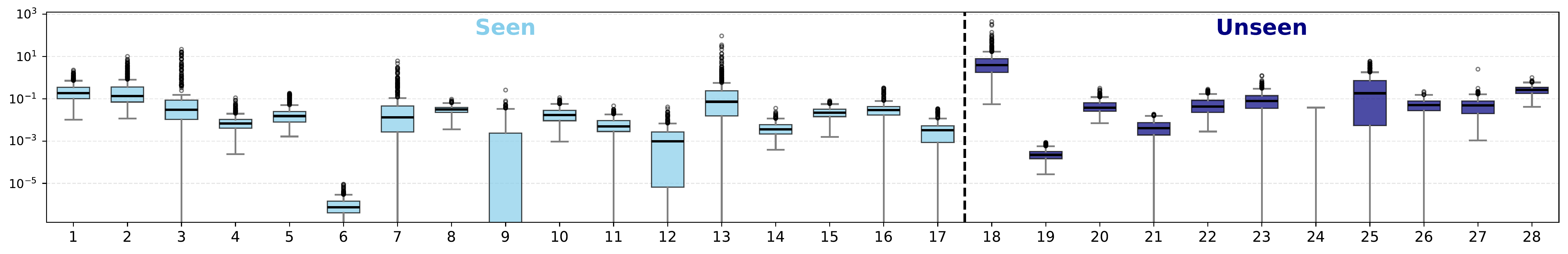
Given a trained controller $\pi_{\phi}$ and system $i$, we report the relative sub-optimality

$$\Delta^{(i)}:=\sum_{j=1}^{J}\frac{\mathcal{J}^{(i)}(x_{0}^{(i,j)};\pi_{\phi})-\mathcal{J}^{(i)}(x_{0}^{(i,j)},\pi^{\star,(i)})}{\mathcal{J}^{(i)}(x_{0}^{(i,j)},\pi^{\star,(i)})},$$ (25)

estimated from rollouts with $J$ random initial conditions. Figure 1 shows the distribution of the relative sub-optimality over the variants across all test systems for the trained transformer controller. The variants are created by perturbing the system matrices $A^{(i)},B^{(i)}$ randomly (entry-wise) around

TABLE II: Seen and unseen LTI systems used in the study.

Seen Systems (17)
1. Inverted Pendulum	2. Simple Pendulum	3. Segway Robot
4. Two Link Arm	5. Mass Spring Damper	6. Suspension System
7. DC Motor	8. Three Link Manipulator	9. Differential Drive Robot
10. SCARA Robot	11. Omnidirectional Robot	12. Cable Driven Robot
13. Flexible Joint Robot	14. Six DOF Manipulator	15. Dual Arm Robot
16. Double Integrator	17. Lotka Volterra
Unseen Systems (11)
18. Asymmetric Oscillator	19. Active Mass Damper	20. Coupled Oscillators
21. Damped Oscillator	22. Triple Mass Spring	23. Electromechanical Actuator
24. Thermal System	25. Fluid Tank	26. Vibrating Beam
27. Motor Generator	28. Mechanical Linkage

$\delta=\pm 30\%$ of their nominal values. For each LTI system, we generate 20 perturbed systems. We report the performance of the transformer across 25 trajectories of each perturbed system. Across the entire family, the transformer remains stabilizing and achieves small sub-optimality. Moreover, the distributions of seen and fine-tuned unseen systems are similar, indicating that the learned mapping generalizes across systems rather than memorizing per-system data. Nevertheless, although able to stabilize it, the transformer achieves relatively less optimal performance when controlling the variants of system 18 (asymmetric oscillator). This is due to poles with very low damping that were not present in the training dataset.

Figure 1: Relative sub-optimality distribution across seen and unseen systems (see Table II for systems’ labels).

Figures 2, 4 and 3 show the performance of the proposed controller across sampled systems. Each figure shows the states on the left and the control input on the right. Figure 2 shows the performance on a seen system. The transformer can closely follow the optimal controller command and settle the system with almost the same transient performance. This shows the capabilities of our method to act as a generalizable optimal controller. Figure 3 illustrates the system’s performance on an unseen system after fine-tuning. The transformer can mimic the optimal controller for this system. This illustrates the performance of our method on unseen systems. Although systems with very low damped poles were not present in the dataset, our method is able to at least stabilize the variants of system 18 as shown in Figure 4.

Lastly, we assess the sensitivity of the proposed framework. Figure 5 (left) shows the validation loss versus the history length $w$. Increasing $w$ improves performance for short windows, followed by a saturation regime. This supports the interpretation that the history window enables implicit system identification. Beyond $w=12$, the gains become marginal. We therefore choose $w=12$ as a practical trade-off between performance and computational cost. Figure 5 (right) shows the validation loss versus the number of training sequences per system. As this number increases, the training data better captures system behavior, leading to lower validation loss.

VI Conclusions

This work presents a supervised framework in which a transformer is trained on optimal trajectories from many linear systems to generalize near-optimal control on these systems. Empirically, the policy achieves small relative sub-optimality over most tested families and remains stabilizing under moderate parameter perturbations, with some degradation on the most challenging family. The framework also supports lightweight few-shot fine-tuning on unseen systems, enabling rapid adaptation when minimal data are available. The main limitation is that generalization is established experimentally rather than certified. Future work will address theoretical stability and robustness guarantees.

Figure 2: Performance on dual arm robot (system #15, seen).

Figure 3: Performance on vibrating beam (system #26, unseen).

Figure 4: Performance on asymmetric oscillator (system #18, unseen).

Figure 5: Ablation study on the effect of (left) the window length and (right) the number of sequences per system

References

- [1] (1990) Optimal control: linear quadratic methods. Prentice Hall. Cited by: §I, §II-A, §III.
- [2] (2023-07) RT-1: robotics transformer for real-world control at scale. In Proceedings of Robotics: Science and Systems, Daegu, Republic of Korea. Cited by: §II-B.
- [3] (2024) A survey on evaluation of large language models. ACM transactions on intelligent systems and technology 15 (3), pp. 1–45. Cited by: §II-C, §IV-C.
- [4] (2021) Decision transformer: reinforcement learning via sequence modeling. Advances in neural information processing systems 34, pp. 15084–15097. Cited by: §II-C.
- [5] (2025) Scaling cross-embodied learning: one policy for manipulation, navigation, locomotion and aviation. In Conference on Robot Learning, pp. 496–512. Cited by: §II-B.
- [6] (2023) Can transformers learn optimal filtering for unknown systems?. IEEE Control Systems Letters 7, pp. 3525–3530. Cited by: §II-C.
- [7] (2025) RAPTOR: a foundation policy for quadrotor control. arXiv preprint arXiv:2509.11481. Cited by: §II-B.
- [8] (2022) Transformers for modeling physical systems. Neural Networks 146, pp. 272–289. Cited by: §II-C.
- [9] (2016) Gaussian Error Linear Units (GELUs). arXiv preprint arXiv:1606.08415. Cited by: §II-C, §IV-C.
- [10] (1999) Neural network control of robot manipulators and nonlinear systems. Taylor & Francis. Cited by: §II-B.
- [11] (2024) Open x-embodiment: robotic learning datasets and rt-x models: open x-embodiment collaboration 0. In IEEE International Conference on Robotics and Automation, pp. 6892–6903. Cited by: §II-B.
- [12] (2024) Octo: an open-source generalist robot policy. CoRR abs/2405.12213. Cited by: §II-B.
- [13] (2018) Sim-to-real transfer of robotic control with dynamics randomization. In International Conference on Robotics and Automation, pp. 3803–3810. Cited by: §II-B.
- [14] (1988) Analysis and design of gain scheduled control systems. Ph.D. Thesis, Massachusetts Institute of Technology. Cited by: §II-A.
- [15] (2017) Attention is all you need. Advances in neural information processing systems 30. Cited by: §II-C, §IV-C.
- [16] (2025) Quattro: transformer-accelerated iterative linear quadratic regulator framework for fast trajectory optimization. In IEEE 64th Conference on Decision and Control, pp. 6629–6636. Cited by: §II-C.
- [17] (2025) Anycar to anywhere: learning universal dynamics model for agile and adaptive mobility. In IEEE International Conference on Robotics and Automation, pp. 8819–8825. Cited by: §II-B.
- [18] (2017) Preparing for the unknown: learning a universal policy with online system identification. In Proceedings of Robotics: Science and Systems, Cited by: §II-B.
- [19] (1996) Robust and optimal control. Prentice Hall. Cited by: §II-A.