Forecast-Aware Cooperative Planning on Temporal Graphs under Stochastic Adversarial Risk

Abstract

Cooperative multi-robot missions often require teams of robots to traverse environments where traversal risk evolves due to adversary patrols or shifting hazards with stochastic dynamics. While support coordination—where robots assist teammates in traversing risky regions—can significantly reduce mission costs, its effectiveness depends on the team’s ability to anticipate future risk. Existing support-based frameworks assume static risk landscapes and therefore fail to account for predictable temporal trends in risk evolution. We propose a forecast-aware cooperative planning framework that integrates stochastic risk forecasting with anticipatory support allocation on temporal graphs. By modeling adversary dynamics as a first-order Markov stay-move process over graph edges, we propagate the resulting edge-occupancy probabilities forward in time to generate time-indexed edge-risk forecasts. These forecasts guide the proactive allocation of support positions to forecasted risky edges for effective support coordination, while also informing joint robot path planning. Experimental results demonstrate that our approach consistently reduces total expected team cost compared to non-anticipatory baselines, approaching the performance of an oracle planner.

I Introduction

Many multi-robot missions, including search-and-rescue and convoy protection, require teams of robots to cooperatively navigate environments where traversal conditions evolve due to adversary patrols or shifting hazards whose motion follows stochastic dynamics. As adversaries or hazards relocate over time, the set of risky regions changes, altering the cost of traversal across the environment. In these settings, support coordination—where robots temporarily delay their own progress to assist or cover teammates traversing risky regions—is a critical mechanism for reducing total team cost. By coordinating support, robots can safely traverse high-risk regions that would otherwise be expensive without teammate assistance [1].

However, the effectiveness of such coordination critically depends on the team’s ability to anticipate when and where these risks will manifest. A myopic planner that only reasons about current risk estimates cannot take advantage of predictable temporal trends. As a result, support actions may be deployed too early, too late, or at locations that cease to be risky, leading to redundant detours and increased total mission cost. Effective support coordination in these dynamic scenarios, therefore, requires reasoning about how risk evolves over time in order to determine when and where assistance will be most beneficial.

Figure 1: From static to stochastic adversaries in multi-robot graph traversal: Static adversaries result in fixed risky edges (left), whereas adversaries with stochastic stay–move dynamics induce dynamic edge risks (right), motivating anticipatory support coordination.

Existing support-based frameworks [1, 2] are primarily designed for static graph environments where adversarial risk remains time-invariant. In these deterministic formulations, support coordination is defined for traversal of fixed risky regions through assistance from predefined support positions [1] as well as formations and teaming [2]. As a result, they do not explicitly model or anticipate temporal risk evolution induced by adversary dynamics, and remain limited to coordinating support between teammates over static risk landscapes.

To address this limitation, we formulate cooperative multi-robot traversal on temporal graphs under stochastic adversarial risk (Fig.1). In our formulation, traversal costs are induced by edge-level adversary dynamics that evolve according to a first-order Markov stay-move process. By propagating these transitions forward in time, we obtain time-indexed edge-risk forecasts over a finite planning horizon. These risk forecasts guide the allocation of support node positions to anticipated risky edges for effective support coordination and induce time-varying edge costs that inform routing decisions during joint path planning. Our main contributions are as follows:

• We formulate cooperative multi-robot traversal on temporal graphs under stochastic adversarial risk, where traversal costs evolve based on adversary dynamics.

• We introduce a forecast-aware support allocation mechanism that leverages adversary stay–move transitions to anticipate edge risk and proactively allocate the most effective support node positions to forecasted risky edges.

• We show that our approach consistently reduces the expected team cost relative to non-anticipatory support allocation baselines and achieves performance close to that of an oracle planner.

II Related Work

We review related work in classical Multi-agent Path Finding (MAPF), temporal graph planning, stochastic shortest paths, game-theoretic graph traversal, and MAPF extensions with risk and support in static settings.

II-A Classical MAPF with Collision Avoidance

Classical MAPF research focuses on collision avoidance in static environments. Optimal solvers such as CBS [3] and Cooperative A* [4], along with learning-based approaches like PRIMAL [5] and prioritized planning [6], aim to minimize makespan or flowtime under fixed edge costs. These formulations do not model evolving traversal risk or cooperative cost mitigation actions, which are central to our work.

II-B Time-Expanded and Time-Varying Graphs

Planning on temporal graphs has been studied in the context of time-dependent shortest path problems [7, 8, 9] and time-expanded graphs for multi-agent settings [10, 11]. While these approaches capture time-varying connectivity or costs, they typically assume deterministic evolution. In contrast, we consider traversal costs driven by stochastic adversarial movement, resulting in non-deterministic, time-varying edge risk.

II-C Stochastic Shortest Paths

The stochastic shortest path framework models uncertainty through probabilistic edge outcomes or costs [12]. Extensions to MAPF incorporate stochastic delays and chance constraints [13, 14, 15, 16, 17]. However, these methods generally assume stationary uncertainty models. Our formulation instead captures non-stationary risk that evolves over time according to known stochastic dynamics.

II-D Game-Theoretic Planning on Graphs

Game-theoretic approaches study adversarial dynamics on graphs, including patrolling games [18, 19], pursuit–evasion problems [20, 21], and adversarial cost manipulation [22]. These work typically assume rational adversaries and two-sided optimization. Our work adopts a one-sided optimization perspective where adversaries follow stochastic movement patterns that induce time-varying risk rather than strategic responses.

II-E MAPF extensions with Risk and Support

The most closely related work extends MAPF with risk and cooperative support. Team Coordination on Graphs with Risky Edges (TCGRE) by Limbu et al. [1] introduces fixed risky edges and predefined support nodes, while Dimmig et al. [2] model team-dependent deterministic costs via overwatch, teaming and formations. These approaches assume static or deterministic risk. We generalize them by introducing stochastic, temporally evolving edge risk and forecast-aware support allocation.

Overall, our work is built on temporal graph reasoning, stochastic risk modeling, and cooperative support coordination within a forecast-driven planning framework, enabling anticipatory coordination under stochastically evolving traversal risk.

III Problem Formulation

We formalize cooperative multi-robot traversal on a graph populated by adversaries that move along edges with stochastic dynamics, inducing time-varying traversal risk.

III-A Robots and Environment

We consider a temporal graph $G=(V,E,\{c_{t}\}_{t=0}^{T})$ with discrete time $t=0,1,\dots,T$, where each $c_{t}:E\to\mathbb{R}_{\geq 0}$ assigns a time-dependent cost $c_{t}(u,v)=c((u,v),t)$ to every edge $(u,v)\in E$. For each node $u\in V$, let $\mathcal{N}(u)=\{w\in V:(u,w)\in E\}$ denote its set of neighbors.

There are $N$ robots indexed by $i=1,\dots,N$, each with a start node $s_{i}\in V$ and a goal node $g_{i}\in V$, which can move between nodes over time. Let $x_{i}(t)\in V$ denote the node occupied by robot $i$ at time $t$. At each time step $t$, robot $i$ selects an action $a_{i}(t)\in\{\mathrm{wait},\mathrm{move},\mathrm{support}\}.$

The robot’s state then evolves as:

$$x_{i}(t{+}1)=\begin{cases}x_{i}(t),&a_{i}(t)=\mathrm{wait}\ \text{or}\ a_{i}(t)=\mathrm{support},\\[4.0pt] v,&a_{i}(t)=\mathrm{move}(u,v),\ x_{i}(t)=u.\end{cases}$$

Although both $\mathrm{wait}$ and $\mathrm{support}$ keep the robot at its current node, the $\mathrm{support}$ action activates edge coverage to reduce traversal risk for teammates (Sec. IV-C), whereas wait provides no such effect.

This discrete-time formulation expands the graph over time, where each node represents a robot’s position at time $t$ and transitions correspond to the robot’s selected action ($\mathrm{wait},\mathrm{move},\mathrm{support}$).

III-B Adversary dynamics

There are $M$ adversaries indexed by $j=1,\dots,M$, each occupying one edge $e=(u,v)\in E$ at any time. For edges $e=(u,v)$ and $e^{\prime}=(u^{\prime},v^{\prime})$, we write $e^{\prime}\sim e$ if they share a common node.

Let $e^{j}_{t}$ denote the random edge occupied by adversary $j$ at time $t$. At each step, an adversary either stays on its current edge or moves to an adjacent edge according to stochastic process $\theta$:

$$\Pr[e^{j}_{t+1}=e\mid e^{j}_{t}=e]\triangleq\theta_{\mathrm{stay}}(e),$$

$$\Pr[e^{j}_{t+1}=e^{\prime}\mid e^{j}_{t}=e]\triangleq\theta_{\mathrm{move}}(e\to e^{\prime}),\qquad e^{\prime}\sim e.$$

These probabilities satisfy the normalization constraint

$$\theta_{\mathrm{stay}}(e)+\sum_{e^{\prime}\sim e}\theta_{\mathrm{move}}(e\to e^{\prime})=1,$$

which defines a first-order Markov chain over the edge set $E$, where transitions occur only between adjacent edges sharing a common node [23].

In this paper, we assume transitions are distributed uniformly across adjacent edges. If $d$ is the number of neighbors of $e$ (excluding $e$ itself), then the probability becomes

$$\theta_{\mathrm{move}}(e\to e^{\prime})=\frac{1-\theta_{\mathrm{stay}}(e)}{d},\qquad\forall e^{\prime}\sim e,\;e^{\prime}\neq e,$$

and zero otherwise.

We define $\gamma^{A}_{uv}(t)\in\{0,1\}$ as the binary indicator that at least one adversary is present on edge $e=(u,v)$ at time $t$. We define the corresponding edge risk probability as its expectation:

$$\rho_{uv}(t)\triangleq\mathbb{E}[\gamma^{A}_{uv}(t)]=\Pr\!\Bigg[\bigcup_{j=1}^{M}\{e^{j}_{t}=(u,v)\}\Bigg]\in[0,1].$$

The exact computation of $\rho_{uv}(t)$ is given in Sec. IV-B

III-C Support model

We define support as a coordinated action among robots, where teammates mitigate the traversal risk induced by adversaries by occupying designated support node positions and taking support action, while other teammates traverse the adversary-occupied edge.

Let $V_{\mathrm{sup}}\subseteq V$ denote the subset of nodes that can serve as support node positions. Each support node $x\in V_{\mathrm{sup}}$ has an associated support set $\mathcal{S}(x)\subseteq E$ (e.g., determined by sensing or communication range constraints) of edges that can be covered from $x$. At time $t$, an edge $(u,v)\in E$ occupied by an adversary is supported if (i) some robot traverses $(u,v)$ at time $t$, and (ii) at least one teammate is positioned at a node $x\in V_{\mathrm{sup}}$ with $(u,v)\in\mathcal{S}(x)$ and takes the $\mathrm{support}$ action at time $t$.

We introduce a binary variable $\gamma^{S}_{uv}(t)\in\{0,1\}$, where $\gamma^{S}_{uv}(t)=1$ indicates that support is active for traversals of $(u,v)$ at time $t$ and $\gamma^{S}_{uv}(t)=0$ otherwise. A robot located at $x$ provides support coverage for all edges $(u,v)\in\mathcal{S}(x)$ simultaneously; hence, $\gamma^{S}_{uv}(t)$ does not track which or how many robots provide support, only whether support is active on the edge $(u,v)$.

The support allocation strategy is described in Sec. IV-C.

III-D Action costs

Let $r_{a}>0$ denote the base traversal cost, and let $r_{p}>0$ represent the additional penalty incurred when traversing an adversary-occupied edge.

The traversal cost for edge $(u,v)$ at time $t$ is:

$$c_{\mathrm{move}}\big((u,v),t;\gamma^{A},\gamma^{S}\big)=r_{a}+r_{p}\,\gamma^{A}_{uv}(t)\,(1-\gamma^{S}_{uv}(t)).$$ (1)

Waiting at a node incurs a constant cost:

$$c_{\mathrm{wait}}(t)=w(t),\qquad w(t)>0,$$ (2)

Supporting at a node incurs a constant cost:

$$c_{\mathrm{support}}(t)=s(t),\qquad s(t)>0.$$ (3)

Upon arrival at $g_{i}$, the robot enters a goal state and incurs no further cost. The per-robot action cost then becomes:

$$c^{(i)}_{\mathrm{act}}(t)=\begin{cases}c_{\mathrm{move}}\big((u,v),t;\gamma^{A},\gamma^{S}\big),&a_{i}(t)=\mathrm{move}(u,v),\\[4.0pt] c_{\mathrm{wait}}(t),&a_{i}(t)=\mathrm{wait},\\[4.0pt] c_{\mathrm{support}}(t),&a_{i}(t)=\mathrm{support},\\[4.0pt] 0,&x_{i}(t)=g_{i}.\end{cases}$$ (4)

Remark. Small positive costs $w(t),s(t)\geq 0$ are used to prevent degenerate strategies (e.g., indefinite waiting or cost-free support behavior), while keeping traversal risk the primary contributor to total cost in our experiments.

III-E Team objective

We define the joint state at time $t$ as:

$$s(t)=(x_{1}(t),\dots,x_{N}(t),\gamma^{A}(t),\gamma^{S}(t)),$$

where $\gamma^{A}(t)=\{\gamma^{A}_{uv}(t):(u,v)\in E\}$ denotes binary adversary presence and $\gamma^{S}(t)=\{\gamma^{S}_{uv}(t):(u,v)\in E\}$ denotes binary support activation. Together, these variables encode the robots’ positions, adversary occupancy on edges, and the activation of support protection on those edges.

A joint policy $\pi$ maps joint states to joint actions as:

$$\pi:\;s(t)\;\mapsto\;(a_{1}(t),\dots,a_{N}(t)),$$

where each $a_{i}(t)\in\{\mathrm{move},\mathrm{wait},\mathrm{support}\}$. The mapping is subject to feasibility constraints: i) a robot may move only to adjacent nodes in $G$, ii) A support action that covers edge $(u,v)$ at time $t$ is valid only if some robot traverses $(u,v)$ at time $t$, and at least one teammate is located at $x\in V_{\text{sup}}$ with $(u,v)\in S(x)$.

The team planning objective is thus:

$$J_{\text{real}}=\min_{\pi}\;\mathbb{E}\!\Bigg[\sum_{t=0}^{T}\sum_{i=1}^{N}c^{(i)}_{\mathrm{act}}(t)\Bigg].$$ (5)

Variants of this objective can also include risk-sensitive criteria (e.g., variance or CVaR of costs), but in the base formulation we minimize expected cumulative cost.

IV Method

Time-varying edge costs induced by stochastic adversary movement make exact planning intractable, as it would require reasoning over all joint robot–adversary realizations. We, therefore, adopt a forecast-based approach that propagates adversary stay-move dynamics forward in time to generate edge-risk forecasts used for both support allocation and joint planning.

IV-A Overview and Pipeline

Figure 2: Forecast-aware cooperative planning pipeline. The graph (left) has adversaries with stochastic dynamics $\theta$. The initial edge risks $\rho_{uv}(0)$ are propagated to forecast time-dependent risks $\rho_{uv}(t)$ (red, middle). These forecasts guide support allocation, producing support-edge mappings $\Gamma_{uv}$ (green, middle). The resulting Forecast-aware temporal graph (right) enables planning with dynamic support activations to minimize expected team cost under stochastic risk.

The proposed framework integrates three stages: adversarial risk forecasting, forecast-informed support allocation, and risk-aware joint planning on a temporal-graph (Fig. 2). First, adversary movement dynamics are propagated forward in time using an edge-to-edge transition model (Sec. IV-B), producing time-indexed edge risk forecasts. Second, these risk forecasts guide the allocation of support nodes to the forecasted risky edges through a scoring-based selection rule (Eqn. (6)) that accounts for spatial proximity, forecasted risk exposure, and robot path relevance (Sec. IV-C). Finally, planning is performed on the resulting temporal graph to minimize expected traversal cost under time-varying edge costs induced by forecasted risks (Sec. IV-D). This pipeline enables anticipatory coordination, allowing robots to plan cooperatively under evolving adversarial risk.

IV-B Adversary-Induced Edge Risk Forecast

Given the adversary stochastic dynamics $\theta$ defined in Sec. III-B, we propagate the initial adversary distributions $\rho_{uv}(0)$ forward in time to obtain edge-risk forecasts $\rho_{uv}(t)$. Each adversary is modeled as a Markov process evolving over edges according to the stay-move transition model $\theta$. This evolution is captured by the edge-to-edge transition matrix $\Theta\in\mathbb{R}^{|E|\times|E|}$, with each entry $\Theta_{e^{\prime},e}$ defined as:

$$\Theta_{e^{\prime},e}\;=\;\theta_{\mathrm{stay}}(e)\,\mathbb{I}[e^{\prime}=e]+\theta_{\mathrm{move}}(e\!\to\!e^{\prime})\,\mathbb{I}[e^{\prime}\sim e],$$

where $\mathbb{I}[\cdot]$ is the indicator function and $e^{\prime}\!\sim\!e$ denotes the two edges share a common node.

For each adversary $j\in\{1,2,..,M\}$, let $q^{(j)}_{uv}(t)\in[0,1]^{|E|}$ denote the marginal probability that adversary $j$ occupies edge $e=(u,v)$ at time $t$. This marginal distribution is propagated over the horizon $T$ as:

$$q^{(j)}_{uv}(t+\tau)=(\Theta)^{\tau}q^{(j)}_{uv}(t),\qquad\tau=0,1,\dots,T.$$

The resulting edge-risk probability is obtained by combining the independent occupancy distributions of all $M$ adversaries:

$$\rho_{uv}(t+\tau)\;=\;1-\prod_{j=1}^{M}\big(1-q^{(j)}_{uv}(t+\tau)\big),$$

which represents the probability that at least one of the $M$ independent adversaries occupies edge $(u,v)$ at time $t+\tau$. This follows directly from the union probability of independent occupancy events [24].

IV-C Forecast-aware Support Allocation

After forecasting edge risks $\rho_{uv}(t)$, we define a mapping of candidate support nodes for edges expected to become risky over time. Unlike static approaches (e.g., TCGRE [1]) that fix support positions based on $\rho_{uv}(0)$, our method identifies potential support-node-to-edge pairings based on the forecasted risk evolution over horizon $T$. While both our method and TCGRE [1] perform the allocation at the initial planning stage ($t=0$), these candidates are not mandated; they are eligible positions the planner evaluates based on a cost-benefit trade-off during search. This allocation process consists of three phases:

IV-C1 Candidate Support Nodes

We restrict allocation to the set of edges expected to manifest risk over horizon $T$. Let $E_{\text{diff}}=\{(u,v)\in E\mid\exists\,t\leq T\text{ s.t. }\rho_{uv}(t)>0\},$ denote the set of edges with nonzero forecasted risk. For each risky edge $(u,v)\in E_{\text{diff}}$, we define a set of candidate support nodes $C_{uv}$:

$$C_{uv}=\{x\in V_{\mathrm{sup}}:(u,v)\in\mathcal{S}(x),\\ \min(d(x,u),d(x,v))\leq k\}.\\$$

Here, $V_{\text{sup}}\subseteq V$ denotes the set of potential support positions, $\mathcal{S}(x)\subseteq E$ specifies which edges node $x$ can support (e.g., due to sensing or communication limits), and $k$-hop enforces spatial locality. This formulation ensures that support is only considered for nodes in the immediate proximity of forecasted threats.

IV-C2 Node Scoring

To prioritize the most effective positions, each candidate node $x\in C_{uv}$ is assigned a score that balances robot traffic with forecasted risk intensity:

$$\text{Score}(x)=\alpha\,\hat{P}(x)\,\big(1+\beta\,\hat{R}(x)\big),$$ (6)

where

• $\hat{P}(x)$ (Normalized Path Overlap): Defined as $\hat{P}(x)=\dfrac{P(x)}{\max_{y\in V}P(y)}$ where $P(x)=\sum_{i=1}^{N}\mathbb{I}[x\in\text{path}_{i}^{T}]$ counts how many robots’ shortest paths $\text{path}_{i}^{T}$ traverse $x$. This ensures support is placed along high-traffic corridors.

• $\hat{R}(x)$ (Normalized Risk Potential): Defined as $\hat{R}(x)=\dfrac{e^{R(x)}}{\sum_{y\in C_{uv}}e^{R(y)}}$ as a softmax-normalized value derived from the raw risk potential $R(x)$ where

  $$R(x)=\frac{R_{uv}^{\text{tot}}}{1+\min(d(x,u),d(x,v))},\quad R_{uv}^{\text{tot}}=\sum_{t=1}^{T}\rho_{uv}(t).$$

  This term prioritizes nodes that are spatially optimal for covering the cumulative risk expected on edge $(u,v)$.

• $\alpha,\beta$ (Weighting parameters): These parameters (default $\alpha=\beta=1$) allow the system to tune the importance of traffic overlap vs. environmental risk.

IV-C3 Allocation Rule

For each risky edge $(u,v)\in E_{\mathrm{diff}}$, we select the top-$s$ candidate nodes by score:

$$\Gamma_{uv}=\operatorname{arg\,top}_{s}\big\{\text{Score}(x):x\in C_{uv}\big\}.$$

This yields a compact support-edge mapping $\Gamma$ utilized by the temporal-graph planner, where each risky edge is assigned up to $s$ nearby support nodes according to the Forecast-aware scoring function (see Algo. 1).

Algorithm 1 Forecast-Aware Support Allocation

Input: Graph $G=(V,E,\{c_{t}\}_{t=0}^{T})$, risk forecasts $\rho_{uv}(t)$, support sets $\mathcal{S}(x)$, robot paths $\{\text{path}_{i}\}_{i=1}^{N}$, horizon $T$, neighborhood size $k$, supports per edge $s$

Output: Support assignments $\Gamma=\{\Gamma_{uv}\}$

$E_{\mathrm{diff}}\leftarrow\{(u,v)\in E:\exists t\leq T,\rho_{uv}(t)>0\}$
for $(u,v)\in E_{\mathrm{diff}}$ do

2       $C_{uv}\leftarrow\{x\in V_{\mathrm{sup}}:(u,v)\in\mathcal{S}(x),\\ \min(d(x,u),d(x,v))\leq k\}$
   for $x\in C_{uv}$ do

3           compute $\text{Score}(x)$ using Eq. (6)

4     $\Gamma_{uv}\leftarrow\operatorname{arg\,top}_{s}\{\,\text{Score}(x):x\in C_{uv}\,\}$

return $\Gamma$

IV-D Forecast-based Team Objective

Directly solving Eqn. (5) is not possible a priori since the $J_{\text{real}}$ depend on adversary realizations $\gamma^{A}_{uv}(t)$, which are unknown at the time of planning. To obtain tractable approximate solution, we replace unknown realizations $\gamma^{A}_{uv}(t)$ with their expected values, the edge-risk forecasts $\rho_{uv}(t)\in[0,1]$.

Under this expectation, the traversal cost for edge $(u,v)$ at $t$ is:

$$\bar{c}_{\mathrm{move}}\big((u,v),t;\gamma^{S}\big)=r_{a}+r_{p}\,\rho_{uv}(t)\,(1-\gamma^{S}_{uv}(t)).$$ (7)

The per-robot expected action cost is then:

$$\bar{c}^{(i)}_{\mathrm{act}}(t)=\begin{cases}\bar{c}_{\mathrm{move}}\big((u,v),t;\gamma^{S}\big),&a_{i}(t)=\mathrm{move}(u,v),\\[4.0pt] c_{\mathrm{wait}}(t),&a_{i}(t)=\mathrm{wait},\\[4.0pt] c_{\mathrm{support}}(t),&a_{i}(t)=\mathrm{support},\\[4.0pt] 0,&x_{i}(t)=g_{i}.\end{cases}$$ (8)

The approximated team planning objective is thus:

$$J_{\text{exp}}\approx\min_{\pi}\;\mathbb{E}\!\Bigg[\sum_{t=0}^{T}\sum_{i=1}^{N}\bar{c}^{(i)}_{\mathrm{act}}(t)\Bigg].$$ (9)

IV-E Planners

Once edge risk forecasts (Sec. III-B) and support node allocations are computed (Sec. IV-C), robots plan over the resulting temporal graph using a Lazily-Expanded A*(Lazy A*). Instead of expanding all edges upfront, Lazy A* defers risk evaluation until an edge is considered during search. The heuristic assumes base traversal costs $r_{a}$ and applies risk penalties $r_{p}$ only upon expansion, reducing computation in sparse-risk settings while preserving A* optimality. Since the heuristic is risk-blind and considers only base edge costs, it remains admissible.

V Experiments

Figure 3: Main Results. Expected team cost ($J_{\exp}$) across adversary stay probabilities $\{0.2,0.5,0.8,1.0\}$, graph sizes ($|V|\in\{5,10,15,20\}$), and robot–adversary configurations $\{2\times 4,3\times 4,4\times 4\}$. Rows show configurations and columns show graph sizes.

V-A Experimental Setup

Graph Environments. We evaluate on randomly generated undirected graphs of $|V|\in\{5,10,15,20\}$ nodes and edge-to-node ratios $r\in\{1.2,1.4,1.6,1.8\}$.

Robots and Adversaries. Each scenario contains 2, 3, or 4 robots with a fixed set of 4 adversaries. Robots move deterministically between nodes toward assigned goals. Adversaries follow a stochastic stay-move Markov process along edges. We evaluate four adversary stay probabilities $\{0.2,0.5,0.8,1.0\}$, spanning from high to zero mobility.

Task Configurations. We consider two start-goal settings: DSDG (Different Start-Different Goal) is used for all experiments, while SSSG (Same Start-Same Goal) is used only for ablations (V-D2). Adversaries are randomly initialized such that no two adversaries occupy the same edge in both settings.

Horizon. The horizon $T$ is set proportional to the graph size ($T\propto|V|$) for both risk forecasting and planning, ensuring sufficient lookahead and planning time, with a 90-second of maximum runtime limit for all methods.

Support Allocation Parameters. Support nodes are allocated from the k-hop neighborhood ($k$=2) with at most one support node per risky edge ($s$=1) within the horizon $T$.

Traversal Cost. Each edge traversal incurs a base cost $r_{a}=1$. An adversarial encounter incurs penalty $r_{p}=10$.

Evaluation Protocol. For each graph size and stay probability, four independent graph instances are evaluated; for each instance, five independent trials (distinct random seeds) are executed. Each (instance, seed) pair constitutes one run, yielding 4×5=20 runs per stay probability. Results are averaged over these runs. All experiments are conducted on a Mac M1 with 8 GB RAM.

V-B Baselines

We compare our Forecast-aware support allocation method against four baselines. No Risk: Adversarial risk and support nodes are disabled, yielding time-invariant edge costs. This serves as an idealized oracle lower bound on team cost. No Support: Forecasted risk is present but no support nodes allocated. Random: Forecasted risk is present and support nodes selected uniformly at random for edges that become risky within the forecast horizon. TCGRE: Forecasted risk is present and support nodes are allocated only for edges that are risky in the initial snapshot.

For all support-allocation methods (Random, TCGRE, and Forecast-aware) support nodes are selected from candidate nodes within the same $k$-hop neighborhood, ensuring differences arise solely from the support allocation strategy.

Monte Carlo Evaluation (Realized Performance). We use Monte Carlo (MC) simulation to sample adversary trajectories under the same stay-move dynamics $\theta$ and initial risk distribution $\rho_{uv}(0)$ to compute realized team cost to calibrate against expected team cost induced by the risk forecast $\rho_{uv}(t)$ (Sec. V-D.1).

V-C Main Results

V-C1 Quantitative Results

Across all graph sizes, robot-adversary configurations, and adversary stay probability settings shown in Fig. 3, the expected team cost decreases monotonically as the stay probability increases. The No Risk baseline forms the oracle lower bound, while No Support forms the upper bound. Our Forecast-aware method consistently achieves the lowest expected team cost among all support-allocation strategies (Forecast-aware, Random, and TCGRE) and remains closest to the No Risk oracle across stay probabilities 0.2, 0.5, and 0.8, with performance converging across all support-allocation methods in the fully static case (stay = 1.0), where temporal risk forecasting provides no additional benefit, collapsing the support-allocation problem to a deterministic setting.

Wherever TCGRE produces feasible solutions, Random and Forecast-aware consistently outperform it because TCGRE allocates support only to initially risky edges, whereas Random and Forecast-aware place support across all edges that become risky over the horizon. On the smallest 5-node graph, Random appears nearly as effective as or slightly better than the Forecast-aware because most nodes in the graph lie within the k-hop neighborhood of risky edges, making even uninformed selection likely to allocate support nodes in impactful locations. As graph size increases ($V>5$), the candidate space expands, causing Random to place support in low-impact regions, while the Forecast-aware method prioritizes support nodes aligned with predicted risky edges and robot traffic, yielding consistently lower expected team cost.

Overall, these quantitative results confirm that combining temporal risk forecasting with robot traffic-aware node scoring is the primary driver of improved performance.

V-C2 Qualitative Results

Figure 4: Illustrative example on a 5-node graph (stay = 0.8) comparing No Support and the Forecast-aware method.

Fig. 4 illustrates 5-node graph example with two robots (blue) and two adversaries (red, stay=0.8) comparing No Support with our Forecast-aware method, under the same risk forecast and planning horizon ($T=5$). Under No Support, robots respond to the high forecasted risk by waiting near risky corridors when near-term traversal is costly. After an initial position exchange, Robot 1 waits repeatedly at node $C$ before committing to $D$ $(A,C,C,C,D,E)$, while Robot 2 delays at $A$ before moving to $B$ $(C,A,A,A,A,B)$, resulting in higher cumulative cost and delayed goal arrival.

In contrast, Forecast-aware allocates support in advance using the same time-indexed risk forecast, enabling earlier traversal of risky edges. After the same initial position exchange, Robot 1 follows $(A,C,D,D,E)$ while Robot 2 follows $(C,A,A,B,B)$, with coordinated support activated at key stages: Robot 2 supports Robot 1 from node $A$ during traversal of $(C,D)$, Robot 1 supports Robot 2 from node $D$ during traversal of $(A,B)$, and Robot 2 again supports Robot 1 from node $B$ during traversal of $(D,E)$. By leveraging forecast-informed support positions, robots avoid prolonged waiting and traverse risky corridors earlier, reducing team cost by approx. 42% (21.20 to 12.30) and shortening completion time by one step (5 to 4).

V-D Ablations

V-D1 Cost Calibration of the Risk Forecast Model

To evaluate risk forecast accuracy, we compare the expected team cost $J_{\text{exp}}$ predicted by Forecast-aware against the realized team cost $J_{\text{real}}$ obtained from 500 MC simulations of adversary trajectories in Table I. Adversary initial locations are randomly initialized once and then fixed for the graph, while robot start-goal pairs are randomized for each robot-adversary configuration. Across all settings, $J_{\text{real}}$ closely matches $J_{\text{exp}}$, with bounded deviations ($|\Delta|\leq 1.0$). In most cases, $\Delta=J_{\text{real}}-J_{\text{exp}}$ is slightly negative. This occurs because $J_{\text{exp}}$ is computed using expected adversary occupancy probabilities, which distribute risk across multiple edges simultaneously. In contrast, $J_{\text{real}}$ is computed from sampled trajectories where adversaries occupy specific edges at each time step. As a result, $J_{\text{exp}}$ can slightly overestimate the total traversal cost along the planned paths relative to a sampled realization. Under stay = 0.2 with increasing adversaries (Adv $\geq 8$) and robots (Ag $\in\{3,4\}$), increased adversary mobility introduces higher variance in realized trajectories, leading to occasional small positive deviations. Furthermore, these deviations remain consistently small and bounded across stay probabilities and robots-adversaries configurations, confirming that downstream support-allocation results rely on a well-calibrated cost model.

TABLE I: Expected vs. realized team cost ($J_{\text{exp}}$ vs $J_{\text{real}}$) across stay probabilities (stay $\in\{0.2,0.5,0.8\}$), robots (Ag $\in\{2,3,4\}$), and adversaries (Adv $\in\{2,4,6,8\}$) on a 10-node graph ($r=1.6$, $k=2$, and $s=1$). Each $J_{\text{real}}$ averaged over 500 Monte Carlo trials.

Ag	Adv	stay = 0.2			stay = 0.5			stay = 0.8
		$J_{\exp}$	$J_{\text{real}}$	$\Delta$	$J_{\exp}$	$J_{\text{real}}$	$\Delta$	$J_{\exp}$	$J_{\text{real}}$	$\Delta$
2	2	6.63	6.52	-0.11	6.41	6.16	-0.25	5.65	5.34	-0.31
2	4	8.18	8.06	-0.12	8.06	7.93	-0.13	7.09	6.62	-0.47
2	6	9.48	9.30	-0.18	9.21	9.03	-0.18	7.88	7.40	-0.48
2	8	10.77	10.71	-0.06	10.69	10.52	-0.17	9.43	8.56	-0.87
3	2	9.61	9.30	-0.31	9.36	9.12	-0.24	8.74	8.52	-0.22
3	4	11.28	11.06	-0.22	11.29	11.09	-0.20	10.73	10.33	-0.40
3	6	12.64	12.55	-0.09	12.55	12.31	-0.24	11.69	11.03	-0.66
3	8	13.61	14.19	+0.58	13.61	13.41	-0.20	12.80	12.16	-0.64
4	2	11.30	11.06	-0.24	11.06	10.91	-0.15	10.49	10.41	-0.78
4	4	12.29	11.99	-0.30	12.10	11.86	-0.24	11.61	11.46	-0.15
4	6	13.10	12.63	-0.47	12.75	12.44	-0.31	12.08	11.82	-0.26
4	8	14.11	14.18	+0.07	13.09	13.52	-0.37	12.97	12.52	-0.45

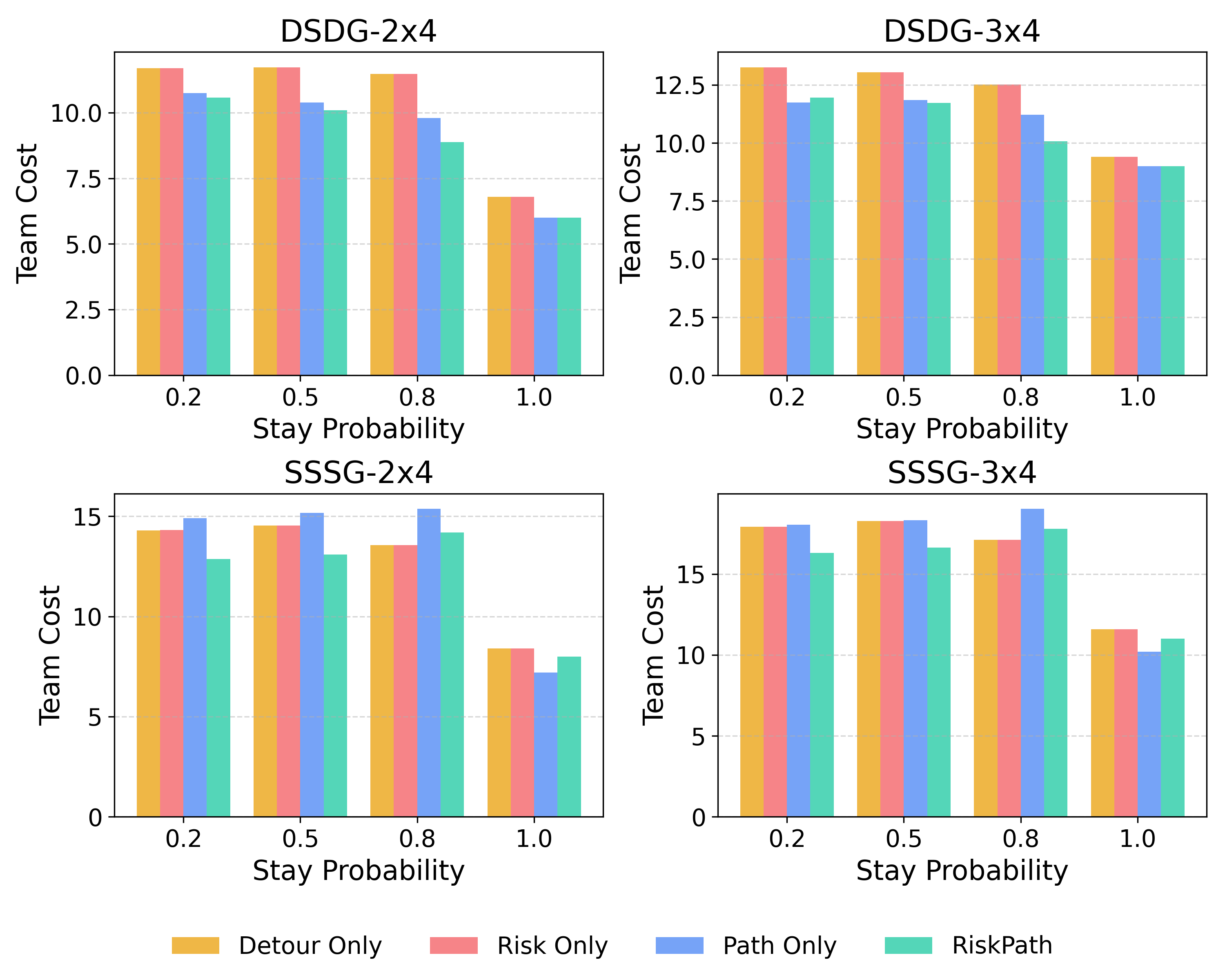
V-D2 Effect of Node Scoring Factors for Support Allocation

Fig. 5 compares four scoring strategies: RiskPath (risk forecast + path overlap), RiskOnly (risk forecast), PathOnly (path overlap), and DetourOnly (proximity). RiskPath (Eq. 6) is used as the default in all main experiments. For this ablation, the same graph setup is used as in Ablation V-D1 across stay probability settings, with both DSDG and SSSG task configurations. Across DSDG scenarios, RiskPath consistently achieves the lowest team cost for stay probabilities 0.2, 0.5, and 0.8, demonstrating the benefit of combining forecasted risk with anticipated robot traffic. At stay = 1.0, PathOnly performs comparably as adversarial risk becomes static and traffic flow dominates support utility. Minor deviations occur under high mobility (e.g., 3×4 at stay = 0.2), where PathOnly occasionally aligns better with realized routes due to high stochasticity of adversarial movement, which reduces the reliability of temporal risk forecasts. In SSSG scenarios, RiskPath performs best at higher mobility (stay $\in\{0.2,0.5\}$), while RiskOnly and DetourOnly become more effective as mobility decreases (stay = 0.8), indicating the increased importance of localized risk and proximity. At stay = 1.0, PathOnly yields the lowest cost, reflecting the dominance of robot traffic in the static case. These results confirm that combining temporal risk forecasts with robot traffic information is most effective in the general DSDG setting (Fig. 3).

Figure 5: Comparison of node-scoring factors across stay probabilities $\{0.2,0.5,0.8,1.0\}$ for DSDG and SSSG scenarios with $2\times 4$ and $3\times 4$ robot-adversary configurations on a 10-node graph ($r=1.6$, $k=2$, $s=1$).

VI Conclusion

We present a forecast-aware support allocation framework for cooperative multi-robot graph traversal under stochastic adversarial risk. By leveraging temporal risk forecasts and anticipated robot path overlap, the proposed method proactively allocates support positions that robots can leverage to reduce expected traversal costs, enabling efficient traversal of high-risk regions without excessive waiting or detouring. Unlike prior static or deterministic formulations, our approach explicitly anticipates risk propagation and places support where it is most effective.

Extensive experiments across multiple graph sizes, robot-adversary configurations, and stochastic regimes show that our method consistently achieves the lowest expected team cost among all non-anticipatory support allocation baselines, while maintaining solution coverage close to the No Risk oracle. Ablation studies further confirm the risk forecast model is well-calibrated and that integrating temporal risk forecasts with robot traffic information is essential for effective support allocation. At 100% stay, the method reduces to TCGRE [1, 25, 26] behavior, confirming correctness in the deterministic setting.

Current limitations include reliance on known adversary dynamics and centralized planning, which restrict application under partial observability or when adversary transition models must be estimated online. Future work will integrate online risk estimation to learn adversary dynamics during execution, and extend the framework to decentralized coordination, investigate scenarios with reactive adversaries, and larger teams over longer planning horizons.

References

- [1] M. Limbu, Z. Hu, S. Oughourli, X. Wang, X. Xiao, and D. Shishika, “Team coordination on graphs with state-dependent edge costs,” in 2023 IEEE/RSJ International Conference on Intelligent Robots and Systems (IROS), pp. 679–684, 2023.
- [2] C. A. Dimmig, K. C. Wolfe, and J. Moore, “Multi-robot planning on dynamic topological graphs using mixed- integer programming,” in 2023 IEEE/RSJ International Conference on Intelligent Robots and Systems (IROS), pp. 5394–5401, 2023.
- [3] G. Sharon, R. Stern, A. Felner, and N. R. Sturtevant, “Conflict-based search for optimal multi-agent pathfinding,” Artificial Intelligence, vol. 219, pp. 1–24, 2015.
- [4] S. Silver, “Cooperative pathfinding,” in Proceedings of the First AAAI Conference on Artificial Intelligence and Interactive Digital Entertainment, AIIDE (A. Nareyek, M. T. J. Spaan, B. Spight, and P. Spronck, eds.), pp. 117–122, AAAI Press, 2005.
- [5] G. Sartoretti, J. Kerr, Y. Shi, G. Wagner, T. K. S. Kumar, S. Koenig, and H. Choset, “Primal: Pathfinding via reinforcement and imitation multi-agent learning,” IEEE Robotics and Automation Letters, vol. 4, no. 3, 2019.
- [6] H. Ma, D. D. Harabor, P. J. Stuckey, J. Li, and S. Koenig, “Searching with consistent prioritization for multi-agent path finding,” in AAAI Conference on Artificial Intelligence, 2018.
- [7] Y. Wang, Y. Yuan, Y. Ma, and G. Wang, “Time-dependent graphs: Definitions, applications, and algorithms,” Data Science and Engineering, vol. 4, pp. 244–259, 2019.
- [8] B. Ding, J. Yang, and X. Qin, “Finding time-dependent shortest paths over large graphs,” in Proceedings of the 11th International Conference on Extending Database Technology, EDBT 2008, Nantes, France, March 25-30, 2008, pp. 273–284, ACM, 2008.
- [9] B. Dean, D. J. Kol, and D. G. Wagner, “Shortest paths in fifo time-dependent networks: Theory and algorithms,” in Proceedings of the 2004 ACM SIGMOD International Conference on Management of Data, (New York, NY, USA), pp. 755–766, ACM, 2004.
- [10] S. Barman and M. Gini, “Multi-agent path finding using time-extended graphs using auctions,” in Proceedings of the International Conference on Robotics and Automation (ICRA), IEEE, 2024.
- [11] Y. Miyamoto, A. Ohya, and T. Ohtani, “A time-dependent risk-aware distributed multi-agent path finder based on a*,” arXiv preprint arXiv:2504.19593, Apr 2025.
- [12] L. Blackmore, M. Ono, A. Bektassov, and B. C. Williams, “A probabilistic particle-control approximation of chance-constrained stochastic predictive control,” IEEE Transactions on Robotics, vol. 26, no. 3, pp. 502–517, 2010.
- [13] M. Ono and B. C. Williams, “An efficient motion planning algorithm for stochastic dynamic systems with constraints on probability of failure,” in AAAI, 2008.
- [14] M. Khonji, R. Alyassi, W. X. Merkt, A. Karapetyan, X. Huang, S. Hong, J. C. Q. Dias, and B. C. Williams, “Multi-agent chance-constrained stochastic shortest path with application to risk-aware intelligent intersection,” ArXiv, vol. abs/2210.01766, 2022.
- [15] D. Atzmon, R. Stern, A. Felner, G. Wagner, R. Barták, and N.-F. Zhou, “Robust multi-agent path finding,” in Proceedings of the 17th International Conference on Autonomous Agents and Multi Agent Systems (AAMAS), pp. 1862–1864, 2018.
- [16] D. Atzmon, R. Stern, A. Felner, G. Wagner, R. Barták, and N.-F. Zhou, “Robust multi-agent path finding and executing,” Journal of Artificial Intelligence Research, vol. 67, pp. 555–591, 2020.
- [17] D. Atzmon, R. Stern, A. Felner, N. R. Sturtevant, and S. Koenig, “Probabilistic robust multi-agent path finding,” in Proceedings of the International Conference on Automated Planning and Scheduling (ICAPS), vol. 30, pp. 29–37, 2020.
- [18] A. Yolmeh and M. Baykal-Gürsoy, “Patrolling games on general graphs with time-dependent node values,” Military Operations Research, vol. 24, no. 2, pp. 17–30, 2019.
- [19] B. Bošanský, V. Lisý, M. Jakob, and M. Pechouček, “Computing time-dependent policies for patrolling games with mobile targets,” in Proceedings of the 10th International Conference on Autonomous Agents and Multiagent Systems (AAMAS), pp. 989–996, IFAAMAS, 2011.
- [20] J.-L. D. Carufel, P. Flocchini, N. Santoro, and F. Simard, “Cops |& robber on periodic temporal graphs,” 2024.
- [21] T. Erlebach, N. Morawietz, J. T. Spooner, and P. Wolf, “A cop and robber game on edge-periodic temporal graphs,” Journal of Computer and System Sciences, vol. 144, p. Article 103534, 2024.
- [22] J. Berneburg, X. Wang, X. Xiao, and D. Shishika, “Multi-robot coordination induced in an adversarial graph-traversal game,” in 2025 IEEE/RSJ International Conference on Intelligent Robots and Systems (IROS), IEEE, 2025.
- [23] J. R. Norris, Markov Chains. Cambridge, UK: Cambridge University Press, 1997.
- [24] S. Thrun, W. Burgard, and D. Fox, Probabilistic robotics. Cambridge, Mass.: MIT Press, 2005.
- [25] M. Limbu, Z. Hu, X. Wang, D. Shishika, and X. Xiao, “Scaling team coordination on graphs with reinforcement learning,” in 2024 IEEE International Conference on Robotics and Automation (ICRA), pp. 16538–16544, IEEE, 2024.
- [26] Y. Zhou, M. Limbu, G. J. Stein, X. Wang, D. Shishika, and X. Xiao, “Team coordination on graphs: Problem, analysis, and algorithms,” in 2024 IEEE/RSJ International Conference on Intelligent Robots and Systems (IROS), pp. 5748–5755, IEEE, 2024.