Make it SING: Analyzing Semantic Invariants in Classifiers

Abstract

All classifiers, including state-of-the-art vision models, possess invariants, partially rooted in the geometry of their linear mappings. These invariants, which reside in the null-space of the classifier, induce equivalent sets of inputs that map to identical outputs. The semantic content of these invariants remains vague, as existing approaches struggle to provide human-interpretable information. To address this gap, we present Semantic Interpretation of the Null-space Geometry (SING), a method that constructs equivalent images, with respect to the network, and assigns semantic interpretations to the available variations. We use a mapping from network features to multi-modal vision language models. This allows us to obtain natural language descriptions and visual examples of the induced semantic shifts. SING can be applied to a single image, uncovering local invariants, or to sets of images, allowing a breadth of statistical analysis at the class and model levels. For example, our method reveals that ResNet50 leaks relevant semantic attributes to the null space, whereas DinoViT, a ViT pretrained with self-supervised DINO, is superior in maintaining class semantics across the invariant space. Code is available at https://tinyurl.com/github-SING.

1 Introduction

State of the art networks, especially vision classifiers, learn internal representations with complex geometry. while this correlates with strong performance on recognition benchmarks, it makes mechanistic interpretability difficult [14, 1]. For example, invariants, derived from the null space of the model’s linear layers, lead to sets of inputs with identical outputs. We refer to these sets as equivalent sets. Whereas nonsemantic invariants such as background or illumination are generally beneficial, invariants that carry semantic information may harm the classifier. However, although users can often introduce image augmentations to increase invariants of certain attributes, they cannot easily determine what the model has actually learned, only via rigorous testing.

This motivates approaches that interpret neural networks while focusing on their geometry. A natural starting point would be the geometry of the classification head, where the last decision is made. A related line of research applies singular value decomposition (SVD) to the latent space based on representative data in the latent feature space [3, 20, 19]; however, these methods are prone to the data covariances rather than network mechanism. Other methods operate directly in the weight-induced null space [11, 47, 32]. For example, the classifier head can be decomposed into two space components:(i) principal directions, associated with dominant singular values that influence the logits; (ii) null directions, the complementary space that keeps the inputs unchanged [43, 2]. While they are able to identify the existence of invariant directions, they fail to explain semantically what they represent, and often rely on task-specific data to demonstrate these directions [32].

Recent advances in mechanistic interpretability [38, 28, 25, 15] leverage the translation of latent features from a given model into a multi-modal vision language space, most notably CLIP [44]. The use of CLIP to compute semantic correlations between text and images facilitates new sets of techniques that focus on producing human-readable concepts and counterfactual examples to aid interpretation. However, to the best of our knowledge, we are the first to map a classifier’s invariant directions into a multi modal network for systematic analysis, providing textual descriptions and visual examples.

We propose a Semantic Interpretation of the Null-space Geometry (SING), a method grounded in SVD of the feature layer to probe the latent feature space of a target classifier and identify the representations of equivalent pairs. The revealed null-space structure is then mapped to CLIP’s vision-language space through linear translators, yielding quantifiable semantic analysis. Our method provides a general framework for measuring human-readable explanations of data invariants, spanning from image and class levels up to entire model assessments. It supports probing, debugging, and comparing these invariants across vulnerable classes and spurious correlations such as background cues, as well as measuring how much a specific concept is ignored by the model. We demonstrate the effectiveness of SING through cross-architecture measurements, per-class analysis, and individual image breakdown. In the last section of our experiments we present a promising direction for null space manipulation, creating features with hidden semantics that the model ignores. Our main contributions are:

• A semantic tool for interpreting invariants. SING links classifier geometry, specifically the null space and the invariants it induces, to meaningful human-readable explanations using equivalent pairs analysis.

• Model comparison. We introduce a protocol to compare different architectures by measuring the leakage of their semantic information into their null space. Our analysis found that DinoViT, among the examined networks, had the least class-relevant leakage into its null space while allowing broad permissible invariants, such as background or color.

• Open vocabulary class analysis. Our framework allows for systematic investigations of the sensitivity of classes to certain concepts. It can discover spurious correlations and assess their contribution. For example, our experiments show that for some spurious attributes in the DinoViT model the classifier head considers them as invariants.

Figure 2: Method Overview. The approach consists of: (a) decomposing the final linear weights to obtain principal and null projectors; (b) training a translator that maps features from the network embedding space to the CLIP image space; (c) creating an equivalent pair to the feature we want to examine. (d) translate the set into CLIP image embedding space, and apply our metrics and visualizations.

2 Related Work

2.1 Explainability through decomposition

Decomposing latent spaces using SVD is a foundational approach for studying their invariances [18]. Aubry and Russell [3] used this technique to probe dominant modes of variation in CNN embeddings, for example illumination and viewpoint, under controlled synthetically rendered scenes. Härkönen et al. [20] applied it to GAN latent spaces for interpretable controls, and more recently Haas et al. [19] used it to present consistent editing directions in diffusion model latent spaces. However, feature-space decomposition is inherently data-dependent: its axes reflect the covariance of the measured dataset rather than the classifier’s decision geometry. Notably, it may miss invariants residing in the classifier’s null space itself.

A complementary study involves decomposing the model weights directly. This line of work includes early low-rank decompositions of convolutional weights for acceleration [27], SVD analyzes of convolutional filters for interpretability [43], and decomposition of the final linear layer to identify the direction relevant to the task and the direction invariant to the task [2]. Null space analysis has been explored across several directions in deep learning. Some works leverage it for information removal: Ravfogel et al. [46] iteratively projected representations onto the null space of a linear attribute classifier to remove protected information while preserving task predictions, while Li and Short [32] exploited null space properties for image steganography, masking images that leave logits unchanged. Others use it as a diagnostic tool: Cook et al. [11] derived OOD detection scores from null space projections, and Idnani et al. [26] explained OOD failures via null-space occupancy, showing that features drifting into the readout’s null space lead to misclassification. Rezaei and Sabokrou [47] further analyzed the last layer null space to quantify overfitting through changes in its structure. Collectively, these methods treat the null space as an operational invariance set for control, detection, and manipulation. However, as far as we know, no current research managed to assign semantic meaning to null directions, as our approach does.

2.2 Projecting features to a vision-language space

Contrastive Language–Image Pretraining (CLIP) [44] learns a rich joint embedding space for images and text, enabling a wide range of vision-language applications. A characteristic property of this space is the presence of a modality gap between image and text embeddings [33]. Beyond its empirical success, the geometry of the CLIP latent space has been studied from multiple perspectives, including geometric analyses [31], probabilistic modeling [7, 6], and asymptotic theoretical analysis [5]. Several methods have leveraged CLIP representations for interpretability, either by mapping classifier features into CLIP’s vision-language space or by using CLIP as supervision to train concept vectors within the target model’s feature space. Text2Concept [38] learns a linear map from any vision encoder to CLIP’s space, turning text prompts directly into concept activation vectors, while CounTEX [28] introduces a bidirectional projection between classifier and CLIP to generate counterfactual explanations. CLIP-Dissect [39] extends this direction to the neuron level, automatically assigning open-vocabulary concept labels to individual neurons by matching their activation patterns to CLIP embeddings. Rather than projecting into CLIP, LG-CAV [25] uses CLIP’s text-image scores on unlabeled probe images as supervision to train concept vectors directly within the target model’s feature space. Taking a broader view, DrML [53], MULTIMON [50], and MDC [10] use language to probe, mine, and correct vision model failures across a range of failure modes. Despite the breadth of these approaches, they all focus on the active feature subspace of the classifier, leaving the null space unexplored.

3 Method

Our method contains several components as can be seen in Figure˜2. We begin by decomposing the target layer into principal and null subspaces and building projection operators that isolate each space. On the second component, we learn a linear mapping that translates the layer’s features into the shared multi-modal space, specifically the image space. We then select a feature and perturb it along a specified semantic direction projected to a chosen subspace, creating the equivalent feature pair. After perturbing, we translate the feature using our translator to observe how its representation changed semantically with visualization and textual measurements. In this section we develop each component in detail, with particular attention to the null space and to the classifier head.

3.1 Setup

In our work, we focus on the last fully connected layer $W\in\mathbb{R}^{c\times m}$, which maps the penultimate features $f\in\mathbb{R}^{m}$ to a logit vector in the dimension of the number of classes $c$. We decompose it with SVD and specifically extract the null space projection matrix $\Pi_{\text{n}}$, which contains all the invariants of the layer. In the translation step we denote $T_{\Theta}(f)$ as the Translator, and we use CLIP as our multi-modal model space. We denote $z^{img}$ and $z^{text}$ as the image and text latent features in CLIP space. We define $\tilde{f}$ as the equivalent pair of $f$ after perturbation in the null space.

3.2 SVD on the classifier head

$W$ can be decomposed into its principal and null spaces via SVD:

$$W=U\,\Sigma\,V^{\top},\qquad V=\bigl[\,V_{\mathrm{p}}\ \ V_{\mathrm{n}}\,\bigr],$$ (1)

where $\Sigma\in\mathbb{R}^{c\times m}$ is a rectangle diagonal matrix containing the singular values in descending order, and $U\in\mathbb{R}^{c\times c}$ and $V\in\mathbb{R}^{m\times m}$ contain the left and right singular vectors, respectively. We take $\operatorname{rank}(W)$, and use it to break the right singular vectors $V$ into the two subspace components, principal space, denoted $V_{\mathrm{p}}$ (associated with non-zero singular values), and the remaining columns $V_{\mathrm{n}}$ that span the null space. Any perturbation $\nu\in\operatorname{span}(V_{\mathrm{n}})$ leaves the logits unchanged:

$$W(f+\nu)=Wf+W\nu=Wf,$$ (2)

since $W\nu=0$ for all $\nu$ in the null space. Consequently, our projector matrices are:

$$\Pi_{\text{p}}=V_{\mathrm{p}}V_{\mathrm{p}}^{\top},\qquad\Pi_{\text{n}}=V_{\mathrm{n}}V_{\mathrm{n}}^{\top}.$$ (3)

3.3 Training a translator

Following Moayeri et al. [38] and justified by Lähner and Moeller [30], we define a linear mapping operator $T:\mathbb{R}^{m}\to\mathbb{R}^{n}$. Recall that $f\in\mathbb{R}^{m}$ is the classifier feature and $z^{img}\in\mathbb{R}^{n}$ the corresponding image feature in CLIP. We fit $T_{\Theta}$ for a certain pretrained model by minimizing a loss combining mean squared error, and weight decay:

$$\mathcal{L}=\|T_{\Theta}(f)-z^{img}\|_{2}^{2}+\lambda\,\|\Theta\|_{2}^{2},$$ (4)

where $\Theta$ is the parameters of the translator and $\lambda$ is a balancing coefficient. Detailed explanations on the training procedure can be found in the supplementary materials. Note that since the translator is linear, it admits $T_{\Theta}(f+v)=T_{\Theta}(f)+T_{\Theta}(v)$ for any $f,v$, hence naturally fits additive feature decompositions, as our framework suggests. The translator is validated to preserve relative classification performance across models, and while we use CLIP as the target space, we demonstrate in the supplementary that other vision-language models can serve this role as well. Although our framework is not limited to linear translators, we empirically verified that this linear map fits well in our setting.

3.4 Metrics

Attribute score.

An angle between two nonzero vectors $x,y$ of the same dimension is defined by:

$$\angle(x,y):=\arccos\bigr(\frac{x\cdot y}{\|x\|\|y\|}\bigl).$$ (5)

CLIP Score, as described in Hessel et al. [23], is the cosine similarity of the angle between a CLIP feature in image space $z^{img}$, and a feature in the text space, $z^{text}$. We write this angle as follows:

$$\angle(z^{img},z^{text})$$ (6)

Recall that $f$ and $\tilde{f}$ are the original and its equivalent pair. We define Attribute Score (AS) for text target $z^{text}$ as the difference between two angles:

$$\text{AS}(f,\tilde{f}|z^{text},T_{\Theta}):=\angle(T_{\Theta}(f),z^{text})-\angle(T_{\Theta}(\tilde{f}),z^{text}).$$ (7)

A positive AS indicates that the equivalent image is semantically closer to the text and vice versa. In our framework, the text prompts are chosen as “an image of a <class>” to analyze how null removal affects classification. However, this metric is general and can be applied with any prompt selection.

Image score.

While AS quantifies how the image deviates from its current semantics, the image may be altered in appearance without affecting AS. Such differences in overall appearance can be measured directly by the angular distance related to the original and its equivalent pair. we define it as Image Score (IS):

$$\text{IS}(f,\tilde{f}|T_{\Theta}):=\angle(T_{\Theta}(f),T_{\Theta}(\tilde{f})).$$ (8)

Intuitively, AS captures the effects of null spaces on the alignment of text-image, whereas IS reflects general semantic changes in the image. When the text is in the correct image class we would like low AS, and hence null-space changes should not affect class distinction. However, a good classifier should allow high IS, and hence large semantic changes that do not affect class distinction, such as background change and other allowed semantic invariants. Details on image synthesis for visualization are provided in the supplementary materials, however it’s highly important to note that those visualizations are used only for qualitative illustration; all quantitative claims rely on logits and CLIP embeddings.

3.5 Applications

Our main focus is on removing the null component from an image feature $f$. This way, the equivalent pair is

$$\tilde{f}=f-\Pi_{\text{n}}f.$$ (9)

Both $f$ and $\tilde{f}$ produce the same logit vector under the examined network, yet the semantic content can be changed as a result of the null-removal process. In the following, we describe how to quantify semantic information leakage at different levels: model, attribute, and image, using the proposed metrics (AS and IS).

Model-level comparison.

A desirable property of well-performing classifiers is to maintain a rich invariant space, while ensuring that this richness does not compromise class preservation. For instance, there exists a wide variety of dogs differing in breed, pose, size, color, background and more, all of which should be classified consistently with high confidence. Hence, the invariant space should support such diversity. However, if perturbations along invariant directions lead to changes in classification confidence or even alter the predicted class, this indicates that class-specific information has leaked into the invariant space - a highly undesirable property that also exposes the model to adversarial vulnerabilities. To evaluate this, we collect a representative set of images (16 ImageNet classes, serving as a proof of concept), compute the AS and IS metrics (with respect to the real class prompt; “an image of a <ground-truth class>”) on all null-removed pairs, and perform a statistical analysis across models. An effective model should exhibit a broad range of IS values, reflecting rich invariance, while maintaining a narrow distribution of AS values, ensuring semantic consistency.

Class and Attribute analysis.

The same methodology can be applied to analyze inter-class behavior by selecting representative sets from different classes. We conducted two complementary variants. First, we collected images from each class independently and computed the absolute Attribute Score (AS) after null-removal, relative to the true label prompt. Higher AS values indicate that the classifier contains more semantic information within the invariant space for that class. This provides a practical diagnostic tool for practitioners when choosing networks suited to specific classes or domains. Second, we expanded the vocabulary to an open set of concepts. We quantified the distance (angles) between the original and the null-removed features, over a broad set of phrases, revealing how semantic correlations emerge between the null space and diverse concepts.

Single image analysis.

Following the same logic, leakage can also be examined at the image level. This provides a fine-grained diagnostic tool for identifying and debugging failure cases.

Null perturbations.

While null removal is useful for fair comparisons across classes, attributes, or images, feature manipulation need not be restricted to a single invariant direction. We propose a more principled selection of perturbation directions. We formalize perturbations that target a specific concept while remaining confined to the model’s invariant (null) subspace. Let $f\in\mathbb{R}^{d}$ be an image feature, $T_{\Theta}:\mathbb{R}^{d}\!\to\!\mathbb{R}^{n}$ the translator into the CLIP image-embedding space, and $z_{\text{text}}\in\mathbb{R}^{n}$ the CLIP text embedding of a prompt (e.g., “an image of a jellyfish”). Define the cosine-similarity score

$$s(f;z_{\text{text}})\;:=\;\frac{\langle z,\,z_{\text{text}}\rangle}{\|z\|\,\|z_{\text{text}}\|}\,,\qquad z:=T_{\Theta}(f).$$ (10)

The semantic direction toward the prompt is the gradient through the translator,

$$g_{\text{text}}(f)\;:=\;\nabla_{f}\,s(f;z_{\text{text}}).$$ (11)

Let $\Pi_{\text{n}}$ denote the orthogonal projector onto the null space ((3)). Projecting this direction onto the null space isolates the component that lives in the invariant subspace:

$$d_{\text{null}}(f)\;:=\;P_{\mathcal{N}}\,g_{\text{text}}(f),\qquad\hat{d}_{\text{null}}(f)\;:=\;\frac{d_{\text{null}}(f)}{\|d_{\text{null}}(f)\|}.$$ (12)

One can control the extent of semantic change via a scalar step size $\varepsilon$ applied to the normalized null direction $\hat{d}_{\text{null}}$:

$$f_{\varepsilon}=f+\varepsilon\,\hat{d}_{\text{null}}(f).$$ (13)

By choosing the prompt to correspond to another class or attribute, this construction probes a class’s sensitivity within the invariant subspace to concepts associated with other classes, thereby revealing “confusing” inter-class relationships.

4 Experiments

(a)

(b)

Figure 3: Model-level comparison (1,000 classes). (a) Attribute Score (AS) quantifies class-dependent semantic leakage into the null space; Image Score (IS) quantifies tolerance to class-independent (non–class-dependent) semantic variation within the invariant subspace. Desirably, AS is low and IS is high (relative to AS). In our results, DinoViT performs best in this regard. (b) We summarize the trade-off with the $\mathrm{IS}/\mathrm{AS}$ ratio (higher is better), DinoViT has the highest ratio and ResNext101 the lowest.

4.1 Dataset and models

We base our analysis on five models pretrained on ImageNet-1k [12] spanning diverse architectures and training paradigms: DinoViT [9], ResNet50 [21], ResNext101 with weakly supervised pretraining [37], EfficientNetB4 trained with Noisy Student [52], and BiTResNetv2 [29]. For statistical analyses, we collect 10k feature vectors per model from all 1,000 ImageNet classes. For each model, we then train a dedicated translator in the same 1,000-class setting. We also empirically confirm that null-space removal leaves logits nearly unchanged, whereas equal-norm perturbations in other directions induce substantial logit and CLIP drift (see supplementary material).

4.2 Model comparison

We compare models globally across all tested classes, measuring AS and IS after null removal. Figure˜3 displays the joint distributions of AS and IS across five models. DinoViT attains the best IS/AS trade-off, consistent with its foundation-scale pretraining on a large, diverse corpus beyond ImageNet prior to fine-tuning. This trade-off is evident both in the IS/AS ratio bar plot (panel (b)) and in the orientation of the confidence ellipses in panel (a). By contrast, ResNext101 shows high AS with substantial variance, which we interpret as class-dependent semantic leakage into its null space. Repeating the comparison with EVA02 [16] as the target multimodal space preserves the same model ordering in the ratio analysis (see supplementary material). To further validate the translator, we train classifier heads on principal features before and after translation to CLIP space, obtaining a high Pearson correlation of 0.972 across models (see supplementary material). We also include an extended 12-model sweep as additional coverage across a broader architectural variety.

4.3 Class analysis

We present per class statistics of AS for two of our models, ResNet50 and DinoViT, and report them class by class; see Figure˜4. For each class, AS is measured after null removal. A complete analysis of the other models can be found in the supplementary materials. DinoViT exhibits stable behavior with very small AS magnitudes (typically $|\mathrm{AS}|<1$), consistent with minimal class-dependent leakage into the null space. By contrast, ResNet50 shows larger and more variable AS across classes. This contrast suggests that DinoViT tends to retain class-relevant semantics within its invariant subspace, whereas ResNet50 appears to possibly rely also on spurious cues, leaving some class-relevant information in the null space. Finally, we observe no significant correlation between the per-class AS rank orderings of the two models, indicating that the effect is model-dependent rather than driven by dataset class structure.

(a) ResNet50

(b) DinoViT

Figure 4: Class Comparison. DinoViT consistently preserves low semantic leakage across classes, whereas ResNet50 exhibits a pronounced imbalance, with certain classes, such as Porcupine and Sports-Car, leaking substantially more semantic information into the null space.

In Fig.˜5, We extend the class analysis to an open vocabulary of concepts. Focusing on DinoViT, we examine two classes, “Arabian Camel” and “Jellyfish”. We measure two quantities: 1) The angle between the translated feature and the CLIP concept embedding; 2) the Attribute Score (AS), quantifies how much content related to a concept resides in the null space; A small AS for loosely related concept can indicate a spurious correlation. Both classes are analyzed through a set contains of 30 concepts, the extreme weakest and strongest are presented. “Arabian Camel” features exhibit little to no AS (short green lines), while Desert attains the smallest CLIP angle among the tested concepts. By contrast, “Jellyfish” features have substantially larger AS, indicating that concepts are tightly coupled to invariances related to this class in the classifier head. The results on the full set of open-vocabulary concepts and intuition for the scale of AS values is provided in the supplementary materials.

(a) ‘Arabian Camel‘ class

(b) ‘Jellyfish‘ class

Figure 5: Open-vocabulary concept analysis. For DinoViT, we sample $\,\sim\!1300$ images per class and compute the CLIP angle (degrees; lower is more similar) to a set of concepts for (a) “Arabian Camel” class and (b) “Jellyfish” class. Blue dots denote original features; red dots denote null-removed (equivalent) features. Green arrows connect each pair and represent the Attribute Score after null removal. Longer arrows indicate larger $|\mathrm{AS}|$ (greater class-dependent semantic leakage); shorter arrows indicate minimal leakage.

Figure 6: Null-space semantic steering (ResNet50). From each original image (left), we add a small perturbation aligned with the indicated prompt (column headers) but constrained to the classifier head’s null space (projected-gradient direction). Although only the invariant component is modified, the feature’s semantics shift toward the target concepts, illustrating how null-space directions can alter meaning without changing the discriminative subspace.

4.4 Gradient direction analysis

In the previous experiments, we restricted our analysis to equivalent pairs obtained by removing the null component. However, our method supports any null-space direction, including text-conditioned perturbations. In Figure˜6, we illustrate concept-directed perturbations confined to the null space of the ResNet50 classifier head. For each original image (left), we follow the CLIP similarity gradient toward a target prompt, project it onto the null space, and take a step in this direction to obtain an equivalent feature. By construction, the perturbed feature leaves the head logits unchanged. The synthesized renderings, generated with UnCLIP [45] for visualization, reveal pronounced semantic shifts toward Arabian Camel, Starfish, Pirate, Jellyfish, and Jeep. This demonstrates the diagnostic value of null-space steering and highlights a security risk: semantics can be manipulated at a single layer while the classifier’s decision remains unaffected.

Table˜1 summarizes null-space steps (calibrated to $\mathrm{IS}=40^{\circ}$) from Sports Car toward the prompt “an image of a jellyfish”. In this setting, DinoViT exhibits low AS, indicating resilience to directed null manipulation. By contrast, EfficientNet and ResNet50 show large AS, suggesting that their null components are easier to steer and that directed invariant perturbations can alter semantics while leaving the logits unchanged.

Table 1: Text-gradient null perturbations. For a fair comparison, each model is perturbed by a fixed null-space step calibrated to $\mathrm{IS}=40^{\circ}$. We report $|\mathrm{AS}|$ toward the target prompt (mean $\pm$ standard deviation; lower is better). DinoViT attains the lowest value (marked in bold), indicating the greatest resistance to directed null-space manipulation, whereas ResNext101 remains comparatively susceptible.

	ResNet50	EfficientNet	BiTresnet	DinoViT	ResNext101
$|\mathrm{AS}|$ towards target	12.04$\pm$0.25	12.38$\pm$0.52	9.19$\pm$0.31	5.0$\pm$0.59	11.15$\pm$0.53

5 Discussion and Conclusion

We introduced SING, a novel approach for analyzing invariances in classification networks. Our method systematically generates equivalent images whose logits are, by construction, identical to those of the original image. We demonstrated a wide range of possible analyses: at the model level, SING facilitates fair sensitivity comparisons across architectures; at the class level, it highlights classes that are less robust to semantic shifts; and at the image level, it aids in debugging failure cases. SING transforms the null space into measurable and human-readable evidence by constructing equivalent pairs, projecting features into a joint vision-language space, and perturbing only the invariant component. In doing so, it reveals how semantics can drift while logits remain fixed, providing a compact diagnostic that complements accuracy at the levels of models, classes, and individual images. Looking ahead, two research directions may help control the null space more directly: (i) Directed augmentation during fine-tuning, encouraging small $\mathrm{AS}$ for essential concepts; (ii) Linear-algebraic control, using projector regularization, rank adjustment, or constrained updates to move useful semantics from the null space to the principal space while preserving logits. SING exposes invariant geometry in a simple, interpretable form, clarifying how semantics can shift while logits remain fixed.

1 Setup and reproducibility

1.1 Translator training

As described in the paper, each translator trained on a specific classifier and its task is to map features from the penultimate layer $f\in\mathbb{R}^{d}$ to a CLIP image feature $e\in\mathbb{R}^{d_{e}}$. Nonlinear translators were trained directly in PyTorch [41], while linear translators were fitted by ridge regression using scikit-learn [42] and then ported to PyTorch for unified inference. The hyperparameters were chosen using sweeps logged in Weights & Biases [8]. We compared three training objectives:

1. Mean squared error (MSE) loss:

   $$\mathcal{L}_{\mathrm{MSE}}(f,e)=\left\lVert T_{\theta}(f)-e\right\rVert_{2}^{2}.$$ (14)

2. Cosine similarity loss:

   $$\mathcal{L}_{\mathrm{cos}}(f,e)=1-\frac{T_{\theta}(f)\cdot e}{\left\lVert T_{\theta}(f)\right\rVert_{2}\left\lVert e\right\rVert_{2}}.$$ (15)

3. MSE + Cosine loss
   

For all three cases, we applied $L_{2}$ regularization. In practice, minimizing $\mathcal{L}_{\mathrm{MSE}}$ alone proved sufficient to achieve high cosine similarity, whereas optimizing $\mathcal{L}_{\mathrm{cos}}$ alone does not reliably reduce MSE, suggesting an asymmetric relationship between the two objectives. This trend is illustrated in Figure˜7.

(a) Cosine-only loss $\mathcal{L}_{\mathrm{cos}}$.

(b) MSE-only loss $\mathcal{L}_{\mathrm{MSE}}$.

(c) Joint loss $\mathcal{L}_{\mathrm{joint}}$.

Figure 7: Training losses for the different translator objectives. Minimizing the MSE loss also improves cosine similarity, whereas cosine-only training leaves the MSE substantially higher.

Our baseline translator is a linear map chosen for stability. To compare linear and non-linear translators, we evaluate three additional. As for Nonlinear architectures, we tried the following combinations:

1. A 3-layer MLP with blocks of the form LayerNorm–GELU–Dropout-FC [4, 22, 49]

2. A 4-layer MLP with the same block.

3. A residual MLP with one residual blocks and one projection layer.
   

All nonlinear translators were optimized with AdamW [36]. with learning rate $1\times 10^{-4}$ and weight decay $\lambda=0.1$.

We report validation results over a 2,000-image subset in Table˜2 and Figure˜8 showing no significant advantage of any non-linear variant over the linear translator.

Table 2: Validation results for different translator architectures on a 2 000-image validation subset from 16 classes. None of the non-linear architectures shows a significant advantage over the linear translator.

Architecture	Mean cosine similarity	Validation MSE
3-layer MLP	0.9049	0.082246
Residual MLP	0.9045	0.082366
4-layer MLP	0.9023	0.084346
Linear	0.8946	0.091355

Figure 8: Cosine similarity distribution of different architectures between the translated and the original CLIP features, over  2k ImageNet features from 16 classes. All the histograms are leaned towards high correlation

2 Null space validation

Let $f$ denote the penultimate classifier feature and $\ell(f)\in\mathbb{R}^{C}$ the corresponding vector of logits for $C$ classes. We define the logit change induced by a perturbation $\delta$ as

$$\Delta_{\ell}(f,\delta)=\left\lVert\ell(f+\delta)-\ell(f)\right\rVert_{2}.$$ (16)

We compare three types of perturbations with matched $\ell_{2}$-norm: (i) a null perturbation $\delta_{\mathrm{null}}$ in the approximate null space of the classifier head, satisfying

$$W\,\delta_{\mathrm{null}}\approx 0,$$ (17)

where $W$ are the head weights; (ii) a random perturbation $\delta_{\mathrm{rand}}$ sampled from an isotropic Gaussian and rescaled to the same norm; and (iii) a principal perturbation $\delta_{\mathrm{principal}}$ chosen along a direction that strongly affects the logits (e.g. a leading sensitive direction for the predicted class) rescaled as well to the null perturbation magnitude. For each type we compute the logit change in L2-norm over a validation set and summarize the distribution in Figure˜9.

As expected, null-space perturbations produce negligible logit changes, while random and principal perturbations have a noticeable shifts. In Figure˜13 we illustrate the corresponding UnCLIP generations for a single feature under these three perturbations and multiple seeds.

(a) Logit change under null vs. random perturbations.

(b) Logit change under principal vs. random perturbations.

Figure 9: Distribution of logit changes $\Delta_{\ell}(f,\delta)$ for null-space, random, and principal perturbations. Null-space perturbations leave logits almost unchanged, whereas principal perturbations induce large logit shifts.

3 Image-level and visualization details

3.1 Angle visual interpretation

For the readers convenience, we provide a visual interpretation of the angles we measured along the paper. For two non-zero vectors $u$ and $v$ we define the angle in degrees

$$\theta(u,v)=\arccos\left(\frac{u\cdot v}{\lVert u\rVert_{2}\,\lVert v\rVert_{2}}\right)\cdot\frac{180}{\pi}.$$ (18)

The attribute score (AS) and image score (IS) used in the main paper are instances of $\theta(\cdot,\cdot)$ applied in CLIP image-embedding space. Figure˜10 provides a concrete mapping between AS/IS values and visual changes for a single example. Angles below roughly $3^{\circ}$ in AS and $10^{\circ}$ in IS correspond to barely perceptible changes, while larger angles produce clear semantic differences such as pose or shape variations.

Image	AS (∘)	IS (∘)
$I_{0}$	0.00	0.0
$I_{1}$	1.58	4.0
$I_{2}$	3.80	10.8
$I_{3}$	4.70	23.0
$I_{4}$	9.48	29.0
$I_{5}$	11.29	36.2

Figure 10: Example images with different attribute scores (AS) and image scores (IS), illustrating the relationship between angular distance and perceived semantic change. Small angles correspond to nearly identical images, while larger angles reflect more significant semantic changes.

3.2 Visualization with UnCLIP

UnCLIP is a two-stage image generator: a prior maps text to a CLIP image embedding, and a diffusion-based decoder with super-resolution modules synthesizes the corresponding image [45]. CLIP encoders normalize image and text embeddings to unit length and compare them using cosine similarity, so semantic information is primarily encoded in the angular component on the unit hypersphere [44].

We use trained translators $T_{\Theta}$ to map classifier features $f$ and their perturbed variants $\tilde{f}$ into the CLIP image-embedding space. Given a feature and its equivalent feature set translated to CLIP, $T_{\Theta}(f)$ and $T_{\Theta}(\tilde{f})$, we rescale the translated equivalent feature to match the norm of the original:

$$\hat{T}_{\Theta}(\tilde{f})=T_{\Theta}(\tilde{f})\,\frac{\left\lVert T_{\Theta}(f)\right\rVert_{2}}{\left\lVert T_{\Theta}(\tilde{f})\right\rVert_{2}}.$$ (19)

This preserves the angular relationships while restoring the radial component, preventing distortions in the visualizations due to radial drift.

To ensure that observed visual differences are solely attributable to changes in the classifier feature $f$, we remove the stochasticity in the diffusion sampling process. We fix the random seed, draw a single Gaussian noise tensor with randn_tensor, scale it by the scheduler’s init_noise_sigma, and reuse this tensor for all images in the batch and for both the decoder and super-resolution stages. For a fixed CLIP image embedding, this procedure yields deterministic outputs.

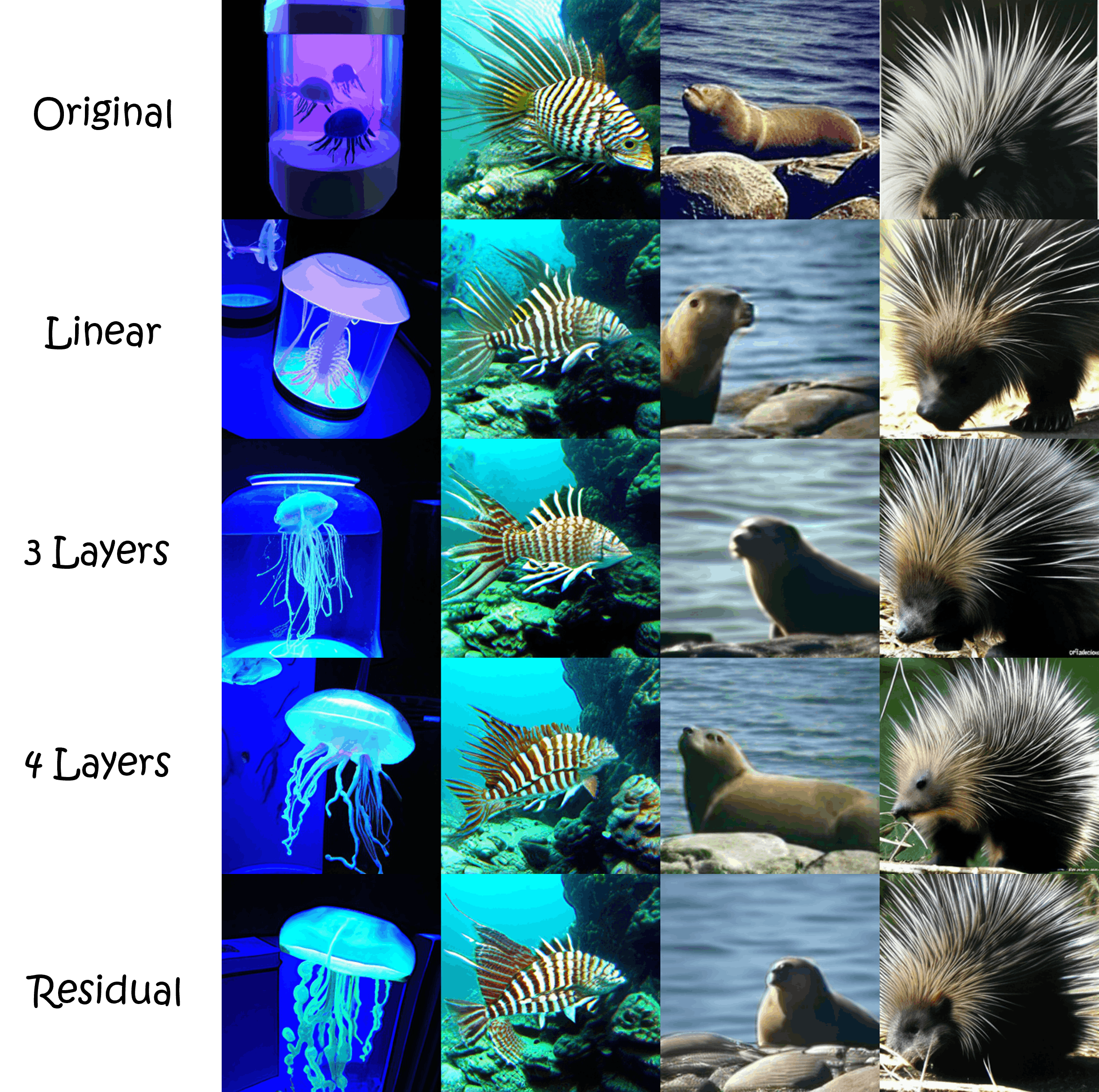
Our implementation uses the Karlo-v1.0.alpha UnCLIP model [13], which follows the original OpenAI framework [45]. The system includes frozen CLIP text and image encoders, a projection layer into the decoder space, a UNet2DConditionModel decoder, two UNet2DModel super-resolution networks, and UnCLIPScheduler instances for both stages. A generation example of the same feature translated by different translators is shown in Figure˜11.

Figure 11: UnCLIP generations from a single classifier feature translated by different translator architectures. Despite small quantitative differences in cosine similarity, the resulting visualizations are qualitatively consistent.

4 Model-level result extensions

We include three additional checks requested during rebuttal integration. First, we repeat the 5-model ratio comparison with EVA02 as the target multimodal space. Second, we expand the ratio comparison from 5 models to 13 models pretrained on ImageNet [12] to increase architectural variety. the list of all models can be found in 3. Third, we evaluate translator robustness by training classifier heads on 500k principal features before and after translation to CLIP space, and computing the model-wise Pearson correlation of classification accuracy. 12. The resulting Pearson score is 0.972, indicating strong consistency between the original-principal and translated-principal feature spaces.

Table 3: List of models from CNNs to ViTs that we used as our test subjects.

Model	ImageNet Top-1 Acc (%)
VGG-16 [48]	71.6
VGG-19 [48]	72.4
DenseNet-121 [24]	74.4
ResNet50 [21]	76.1
DinoViT [9]	84.0
EfficientNet-B0 (NS) [52]	78.7
BiT-ResNet (M-R50x1) [29]	80.4
ResNeXt-101 32x8d (WSL) [37]	82.6
ConvNeXt-Base [35]	85.8
Swin-L [34]	86.3
DINOv2-L [40]	86.5
DeiT-3-L/16 [51]	87.7
EVA-02-L [17]	89.9

(a) 5-model ratio comparison in EVA02 space.

(b) Extended ratio comparison over 12 models.

(c) Translator robustness on principal features (Pearson 0.972).

Figure 12: Additional model-level validations used in the camera-ready update.

Figure 13: UnCLIP generations of a single feature under three perturbation types (null, random, principal) across four random seeds. Null-space perturbations preserve the global class semantics, while random and principal perturbations produce more noticeable semantic changes.

5 Class-level analyses

We provide violin plots for all models that participated in our experiments (Figures˜14(a), 14(b) and 14(c)). Each violin summarizes the distribution of semantic angle changes (in degrees) under null-space perturbations for a given class.

(a) BiT-ResNet [29].

(b) ResNeXt [37].

(c) EfficientNet [52].

Figure 14: Per-class distribution of null-space semantic angle changes across three architectures. Each violin corresponds to a single class; narrow distributions around zero indicate classes largely invariant to null-space perturbations. The consistent pattern across architectures with different inductive biases confirms the generality of our observations.

Figures˜15 and 16 provide extended open-vocabulary concept lists used in the class analyses of the “Arabian Camel” and “Jellyfish” classes in DinoViT. Nodes correspond to text prompts and the target class, and edge strengths reflect CLIP similarity between image and text embeddings. These plots show that the concepts we highlight in the main paper are representative of broader open-vocabulary neighborhoods.

Figure 15: Open-vocabulary analysis for the “Arabian Camel” class in DinoViT. We show a larger set of prompts and their CLIP similarities to the class, illustrating the semantic neighborhood used in our analysis.

Figure 16: Open-vocabulary analysis for the “Jellyfish” class in DinoViT. The graph highlights related concepts and their CLIP similarities, showing that the concepts discussed in the main paper are part of a consistent semantic cluster.

6 DinoViT feature wrapper

We use a wrapper around a pre-trained DinoViT backbone [9] to expose the penultimate feature $f$ and the classifier head weights $W$. We extract the sequence of tokens from the layer immediately before the classifier head (denoted "encoder.ln" in our implementation), take the class token as $f$, and apply the original head to obtain logits $\ell(f)=Wf$.

⬇

class SelectClassToken(nn.Module):

def __init__(self, f):

super().__init__()

self.f, self.B = f, 1

def forward(self, x):

# x: (B * num_tokens, f); reshape and select class token (index 0)

return x.reshape(self.B, -1, self.f)[:, 0, :]

def set_B(self, B=1):

self.B = B

class DinoHookable(nn.Module):

def __init__(self, base: nn.Module, extractor, feature_dim=1024):

super().__init__()

self.extractor = extractor

self.fc = base.heads.head # classifier head; weights are W^T

self.penultimate = SelectClassToken(f=feature_dim)

def forward(self, x: torch.Tensor) -> torch.Tensor:

self.penultimate.set_B(x.size(0))

# token sequence before the classifier head

x = self.extractor.extract(x, "encoder.ln")

# penultimate feature f (class token)

x = self.penultimate(x)

# logits; penultimate feature f is available for analysis

return self.fc(x)

This wrapper allows us to reuse the original DinoViT classifier while directly accessing the feature space in which we construct translators and null-space perturbations.

References

- [1] (2019) Intrinsic dimension of data representations in deep neural networks. External Links: 1905.12784, Link Cited by: §1.
- [2] (2023) Keep moving: identifying task-relevant subspaces to maximise plasticity for newly learned tasks. arXiv preprint arXiv:2310.04741. Cited by: §1, §2.1.
- [3] (2015) Understanding deep features with computer-generated imagery. In Proceedings of the IEEE international conference on computer vision, pp. 2875–2883. Cited by: §1, §2.1.
- [4] (2016) Layer normalization. arXiv preprint arXiv:1607.06450. Cited by: item 1.
- [5] InfoNCE induces gaussian distribution. In The Fourteenth International Conference on Learning Representations, Cited by: §2.2.
- [6] (2026) General and domain-specific zero-shot detection of generated images via conditional likelihood. In Proceedings of the IEEE/CVF Winter Conference on Applications of Computer Vision, pp. 7809–7820. Cited by: §2.2.
- [7] (2025) Whitened clip as a likelihood surrogate of images and captions. In Proceedings of the 42nd International Conference on Machine Learning, Proceedings of Machine Learning Research, Vol. 267, Vancouver, Canada. Cited by: §2.2.
- [8] (2020) Experiment tracking with weights and biases. Note: Software available from https://www.wandb.com/ Cited by: §1.1.
- [9] (2021) Emerging properties in self-supervised vision transformers. In Proceedings of the IEEE/CVF international conference on computer vision, pp. 9650–9660. Cited by: §4.1, Table 3, §6.
- [10] (2025) Model diagnosis and correction via linguistic and implicit attribute editing. In Proceedings of the Computer Vision and Pattern Recognition Conference, pp. 14281–14292. Cited by: §2.2.
- [11] (2020) Outlier detection through null space analysis of neural networks. arXiv preprint arXiv:2007.01263. Cited by: §1, §2.1.
- [12] (2009) Imagenet: a large-scale hierarchical image database. In 2009 IEEE conference on computer vision and pattern recognition, pp. 248–255. Cited by: §4.1, §4.
- [13] (2022) Karlo-v1.0.alpha on coyo-100m and cc15m. Note: https://github.com/kakaobrain/karlo Cited by: §3.2.
- [14] (2017) Towards a rigorous science of interpretable machine learning. External Links: 1702.08608, Link Cited by: §1.
- [15] (2025) Mechanistic understanding and validation of large ai models with semanticlens. Nature Machine Intelligence, pp. 1–14. Cited by: §1.
- [16] (2024) Eva-02: a visual representation for neon genesis. Image and Vision Computing 149, pp. 105171. Cited by: §4.2.
- [17] (2023) EVA-02: a visual representation for neon genesis. arXiv preprint arXiv:2303.11331. Cited by: Table 3.
- [18] (1970) Singular value decomposition and least squares solutions. Numerische Mathematik 14, pp. 403–420. Cited by: §2.1.
- [19] (2024) Discovering interpretable directions in the semantic latent space of diffusion models. In 2024 IEEE 18th International Conference on Automatic Face and Gesture Recognition (FG), pp. 1–9. Cited by: §1, §2.1.
- [20] (2020) GANSpace: discovering interpretable gan controls. In Advances in Neural Information Processing Systems, Cited by: §1, §2.1.
- [21] (2016) Deep residual learning for image recognition. In Proceedings of the IEEE conference on computer vision and pattern recognition, pp. 770–778. Cited by: §4.1, Table 3.
- [22] (2016) Gaussian error linear units (gelus). arXiv preprint arXiv:1606.08415. Cited by: item 1.
- [23] (2021) Clipscore: a reference-free evaluation metric for image captioning. arXiv preprint arXiv:2104.08718. Cited by: §3.4.
- [24] (2017) Densely connected convolutional networks. In Proceedings of the IEEE conference on computer vision and pattern recognition, pp. 4700–4708. Cited by: Table 3.
- [25] (2024) Lg-cav: train any concept activation vector with language guidance. Advances in Neural Information Processing Systems 37, pp. 39522–39551. Cited by: §1, §2.2.
- [26] (2023) Don’t forget the nullspace! nullspace occupancy as a mechanism for out of distribution failure. In The Eleventh International Conference on Learning Representations, Cited by: §2.1.
- [27] (2014) Speeding up convolutional neural networks with low rank expansions. In British Machine Vision Conference (BMVC), pp. 3.1–3.12. External Links: Link Cited by: §2.1.
- [28] (2023) Grounding counterfactual explanation of image classifiers to textual concept space. In Proceedings of the IEEE/CVF Conference on Computer Vision and Pattern Recognition, pp. 10942–10950. Cited by: §1, §2.2.
- [29] (2020) Big transfer (bit): general visual representation learning. In European conference on computer vision, pp. 491–507. Cited by: §4.1, Table 3, 14(a), 14(a).
- [30] (2024) On the direct alignment of latent spaces. In Proceedings of UniReps: the First Workshop on Unifying Representations in Neural Models, pp. 158–169. Cited by: §3.3.
- [31] (2025) The double ellipsoid geometry of clip. In Proceedings of the 42nd International Conference on Machine Learning, Proceedings of Machine Learning Research, Vol. 267, Vancouver, Canada. Cited by: §2.2.
- [32] (2024) Null space properties of neural networks with applications to image steganography. arXiv preprint arXiv:2401.12345. External Links: Link Cited by: §1, §2.1.
- [33] (2022) Mind the gap: understanding the modality gap in multi-modal contrastive representation learning. Advances in Neural Information Processing Systems 35, pp. 17612–17625. Cited by: §2.2.
- [34] (2021) Swin transformer: hierarchical vision transformer using shifted windows. In Proceedings of the IEEE/CVF International Conference on Computer Vision (ICCV), pp. 9992–10002. Cited by: Table 3.
- [35] (2022) A ConvNet for the 2020s. In Proceedings of the IEEE/CVF Conference on Computer Vision and Pattern Recognition (CVPR), Cited by: Table 3.
- [36] (2019) Decoupled weight decay regularization. In International Conference on Learning Representations, Cited by: §1.1.
- [37] (2018) Exploring the limits of weakly supervised pretraining. In Proceedings of the European conference on computer vision (ECCV), pp. 181–196. Cited by: §4.1, Table 3, 14(b), 14(b).
- [38] (2023) Text2concept: concept activation vectors directly from text. In Proceedings of the IEEE/CVF Conference on Computer Vision and Pattern Recognition, pp. 3744–3749. Cited by: §1, §2.2, §3.3.
- [39] (2022) Clip-dissect: automatic description of neuron representations in deep vision networks. arXiv preprint arXiv:2204.10965. Cited by: §2.2.
- [40] (2024) DINOv2: learning robust visual features without supervision. Transactions on Machine Learning Research (TMLR). Cited by: Table 3.
- [41] (2019) PyTorch: an imperative style, high-performance deep learning library. Advances in Neural Information Processing Systems 32, pp. 8024–8035. Cited by: §1.1.
- [42] (2011) Scikit-learn: machine learning in Python. Journal of Machine Learning Research 12, pp. 2825–2830. Cited by: §1.1.
- [43] (2022) The svd of convolutional weights: a cnn interpretability framework. Note: Tech. Report, ResearchGate External Links: Link Cited by: §1, §2.1.
- [44] (2021) Learning transferable visual models from natural language supervision. arXiv preprint arXiv:2103.00020. External Links: Link Cited by: §1, §2.2, §3.2.
- [45] (2022) Hierarchical text-conditional image generation with clip latents. arXiv preprint arXiv:2204.06125 1 (2), pp. 3. Cited by: §3.2, §3.2, §4.4.
- [46] (2020) Null it out: guarding protected attributes by iterative nullspace projection. In Proceedings of the 58th Annual Meeting of the Association for Computational Linguistics, pp. 1688–1703. External Links: Link Cited by: §2.1.
- [47] (2023) Quantifying overfitting: evaluating neural network performance through analysis of null space. arXiv preprint arXiv:2305.19424. External Links: Link Cited by: §1, §2.1.
- [48] (2015) Very deep convolutional networks for large-scale image recognition. In International Conference on Learning Representations (ICLR), Cited by: Table 3, Table 3.
- [49] (2014) Dropout: a simple way to prevent neural networks from overfitting. Journal of Machine Learning Research 15 (1), pp. 1929–1958. Cited by: item 1.
- [50] (2023) Mass-producing failures of multimodal systems with language models. Advances in neural information processing systems 36, pp. 29292–29322. Cited by: §2.2.
- [51] (2022) DeiT III: revenge of the ViT. In Computer Vision – ECCV 2022, Lecture Notes in Computer Science, Vol. 13684, pp. 516–533. Cited by: Table 3.
- [52] (2020) Self-training with noisy student improves imagenet classification. In Proceedings of the IEEE/CVF conference on computer vision and pattern recognition, pp. 10687–10698. Cited by: §4.1, Table 3, 14(c), 14(c).
- [53] (2023) Diagnosing and rectifying vision models using language. arXiv preprint arXiv:2302.04269. Cited by: §2.2.
Supplementary Material