Constraining Small Planet Compositions for Future Missions

Abstract

Accurate mass and radius measurements of small transiting exoplanets are essential for probing their compositions, formation histories, and potential habitability. We present a uniform analysis of six planetary systems (each hosting at least one small transiting planet): K2-79, K2-106, K2-111, K2-222, K2-263, and TOI-1634. Our study combines new CHEOPS transit observations with archival photometry from K2, TESS, and ground-based facilities, alongside new and archival radial velocity data from HARPS-N, HIRES, ESPRESSO, and others. For each system, we perform joint transit and RV modelling, achieving typical precisions better than 15% and 5% for mass and radius, respectively, and thus enabling precise bulk density determinations. These reveal a range of compositions, including rocky planets near the radius valley (e.g. K2-106 b, TOI-1634 b), intermediate-density planets requiring steam-rich or mixed volatile envelopes (e.g. K2-111 b, K2-263 b), and low-density regimes, consistent with gas dwarfs or water-worlds (e.g. K2-79 b, K2-222 b). Several systems show evidence of additional companions detectable via RVs but not seen in transit. The results highlight the value of coordinated CHEOPS and HARPS-N observations in delivering some of the most precise bulk densities for small planets to date and support the preparation for future atmospheric characterisation missions.

1 Introduction

The detailed characterisation of small exoplanets is critical to understanding their formation, evolution, and potential habitability. While transit and RV surveys have revealed thousands of planets across a wide range of masses, radii, and orbital separations, the number of well-characterised small exoplanets ($1<R_{p}<4\,R_{\oplus}$) — those with both masses and radii measured to better than 20% and 5%, respectively — remains limited to fewer than 350 systems (Otegi et al., 2020; Christiansen et al., 2025). These planets exhibit remarkable diversity in composition and atmospheric properties (Madhusudhan, 2019), and their internal structures contain key information about formation pathways, accretion histories, and atmospheric evolution (Mordasini et al., 2012; Dorn et al., 2015; Bean et al., 2021); thus, characterising their internal structures and evolutionary histories remains a central goal for the exoplanet field.

A key step towards this goal lies in accurately determining these planets’ bulk densities. This precision is particularly important in the context of upcoming and future missions. The European Space Agency’s (ESA) PLAnetary Transits and Oscillations of stars (PLATO; Mas-Hesse, 2023) mission, scheduled for launch in 2027, is specifically designed to improve the accuracy of planetary radii, masses, and ages through long-baseline photometry combined with asteroseismology, Gaia astrometry, and high-resolution spectroscopy, targeting precisions of $\sim 5\%$ in radius and $\sim 10\%$ in mass and age. Similarly the Earth2.0 space mission (ET; Ge and The ET team, 2024) aims to detect and characterise Earth-sized planets around Sun-like stars, further expanding the sample of well-characterised small exoplanets by the end of the 2030s. Looking further ahead the Habitable Worlds Observatory (HWO; National Academies of Sciences, Engineering, and Medicine, 2021), currently in the concept phase with a potential launch in the 2040s, will rely heavily on prior knowledge of planetary parameters. HWO aims to characterise planets around nearby Sun-like stars through both direct imaging and spectroscopic observations, including reflected-light spectroscopy of directly imaged planets and, for transiting systems, transmission spectroscopy. Accurate knowledge of a planet’s bulk density, derived from precise measurements of its mass and radius, will be critical for HWO. Such measurements allow scientists to distinguish between rocky, water-rich, and volatile-dominated worlds before direct observation and are essential for interpreting atmospheric spectra in the context of interior composition (Batalha et al., 2019; Salvador et al., 2024; Damiano et al., 2025). This information also improves target selection and assessment of planetary habitability, when considered alongside additional factors such as orbital separation, stellar age, magnetic protection, and the irradiation environment of the host star (Valente et al., 2024; Atkinson et al., 2024; Zhu and Preibisch, 2025; See et al., 2025). In addition, accurate ephemerides, such as the transit centre time, are crucial to ensure that transits are successfully observed and valuable telescope time is not wasted. The exoplanet community’s push towards detecting and characterising potentially habitable worlds thus hinges on refining the planetary parameters of validated small exoplanets.

The HARPS-N Collaboration has played a leading role in the characterisation of small transiting exoplanets, contributing more than a third of the current sample with well constrained masses and radii (Pepe et al., 2013; Mortier et al., 2018; Mayo et al., 2019; Rice et al., 2019; Lacedelli et al., 2021; Rajpaul et al., 2021; Bonomo et al., 2023). To expand this effort, we secured CHaracterising ExOPlanet Satellite (CHEOPS; Benz et al., 2021) observations targeting six such systems, each originally identified by the K2 (Howell et al., 2014) or the Transiting Exoplanet Survey Satellite (TESS; Ricker et al., 2014) missions and actively monitored with HARPS-N under its GTO program. For each target, we obtained two transits with CHEOPS to achieve two complementary goals: (1) refining planetary radius measurements, and (2) improving orbital ephemerides to tighten priors on RV modelling. This strategy enhances the precision of mass determinations by reducing phase uncertainties and improving transit timing predictions. By combining CHEOPS and HARPS-N data with a range of archival photometry and spectroscopy, we present some of the most accurately constrained bulk densities currently available for small exoplanets, providing key insights into their interior structure and atmospheric evolution.

In this work, we present a comprehensive re-analysis of six planetary systems: K2-79, K2-106, K2-111, K2-222, K2-263, and TOI-1634. Each system hosts at least one small transiting planet with existing photometric and spectroscopic observations, and may exhibit compelling features such as planet multiplicity, low densities, and proximity to the radius valley (Owen and Wu, 2013; Lopez and Fortney, 2013; Fulton et al., 2017). Table 1 summarises the stellar and planetary parameters for these targets with the values drawn from previous literature. We compile and uniformly model transit photometry from K2, TESS, CHEOPS, and a range of ground-based instruments, alongside RV datasets from HARPS-N, HIRES, ESPRESSO, HARPS, FIES, PFS, IRD, and HDS, incorporating these literature stellar parameter values as priors in our analysis. The typical precision of these stellar parameters (2–5% in mass; 1–4% in radius) sets the baseline accuracy for the derived planetary masses, radii, and bulk densities, as these quantities scale directly with the host-star properties. Recent studies have demonstrated that modelling stellar spectral energy distributions can further improve stellar radii and masses, enabling planetary radii to be determined to $\sim 2\%$ and masses to $\sim 10\%$ precision (Morrell et al., 2026). While we adopt literature stellar parameters in this work, continued improvements in stellar characteriation will directly translate into tighter constraints on planetary compositions. Our modelling approach incorporates both single- and multi-planet Keplerian fits, Gaussian Process (GP) noise modelling where appropriate, and a consistent treatment of systematics and uncertainties across instruments. This enables a robust derivation of planetary parameters and direct comparisons between systems.

The six systems studied here span a wide range of planetary properties and evolutionary pathways. Several planets, such as K2-106 b and TOI-1634 b, lie near the boundary between rocky super-Earths and volatile-rich sub-Neptunes, probing the effects of extreme irradiation and atmospheric loss (Ginzburg et al., 2018; Gupta and Schlichting, 2020). Others, like K2-79 b and K2-222 b, fall into the low-density regime where compositions are degenerate, highlighting the H/He vs water-rich envelopes (Rogers and Seager, 2010; Zeng et al., 2021). K2-263 b, by contrast, likely formed beyond the snow line and now orbits at a cool enough distance to offer insights into the formation and inward migration of cold sub-Neptunes (Bitsch et al., 2021). Meanwhile, K2-111 b orbits an $\alpha$-enhanced, iron-poor star, raising questions about the link between stellar composition and planet interiors (Santos et al., 2017). Together, these systems provide a valuable testbed for planet formation and atmospheric evolution models, and offer a diverse set of targets for future atmospheric characterisation with upcoming facilities such as HWO.

The paper is structured as follows: Section 2 describes the photometric and spectroscopic datasets used in our analysis. Section 3 outlines our modelling approach for each system, including transit and RV fitting methods. Section 4.1 presents our results for each system, with updated interior structure modelling. In Section 4.2 we discuss implications for future study with upcoming missions. We conclude in Section 5 with a summary and outlook for future work.

Table 1: Stellar and planetary parameters from previous literature. Sources are listed at the bottom of the table. For TOI-1634 b, planetary parameters from two sources are given due to significant differences in reported masses. In this case, *  indicates Cloutier et al. (2021) whilst †  indicates Hirano et al. (2021). $\ddagger$ indicates parameters not reported in the literature. No planet c is known for K2-79 or K2-263. For K2-222 c, the orbital period is reported, but no mass estimate or RV amplitude has been published. For TOI-1634, no confirmed planet c has been detected: Cloutier et al. (2021) and Hirano et al. (2021) both note possible longer-period RV trends, but neither reports a statistically significant or characterised second planet. ‘NT’ indicates a non-transiting planet.

Parameter	K2-79	K2-106	K2-111	K2-222	K2-263	TOI-1634
Astrometry
R.A.	03h41m01.42s	00h52m19.21s	03h59m33.67s	01h05m51.00s	08h38m43.71s	03h45m33.75s
Decl.	+13d31m09.07s	+10d47m40.94s	+21d17m54.69s	+11d45m13.38s	+15d40m50.17s	+37d06m44.21s
$\pi$ [mas]	$3.841\pm 0.015$	$4.0603\pm 0.0499$	$4.9626\pm 0.0674$	$10.0090\pm 0.0608$	$6.1262\pm 0.0514$	$28.512\pm 0.018$
d [pc]	$256.011^{+2.349}_{-2.307}$	$244.590^{+3.044}_{-2.972}$	$200.394^{+2.763}_{-2.690}$	$101.321^{+0.632}_{-0.625}$	$162.481^{+1.380}_{-1.357}$	$35.2736^{+0.0527}_{-0.0526}$
Spectral Type	G1	G5 V	G2	G0	G9 V	M2 V
Photometry
$B$ [mag]	$12.89\pm 0.02$	$12.576\pm 0.443$	$11.80\pm 0.03$	$10.04\pm 0.03$	$12.35\pm 0.03$	$14.755\pm 0.060$
$V$ [mag]	$12.07\pm 0.06$	$12.101\pm 0.031$	$11.14\pm 0.04$	$9.54\pm 0.03$	$11.61\pm 0.04$	$13.24\pm 0.04$
$J$ [mag]	$10.36\pm 0.02$	$10.770\pm 0.023$	$9.77\pm 0.02$	$8.42\pm 0.02$	$10.22\pm 0.02$	$9.564\pm 0.021$
$H$ [mag]	$10.00\pm 0.02$	$10.454\pm 0.026$	$9.48\pm 0.03$	$8.17\pm 0.03$	$9.81\pm 0.02$	$8.940\pm 0.021$
$K$ [mag]	$9.91\pm 0.02$	$10.344\pm 0.021$	$9.38\pm 0.02$	$8.11\pm 0.02$	$9.75\pm 0.02$	$8.699\pm 0.014$
Atmospheric parameters
$T_{\rm eff}$	$5897\pm 118$	$5532\pm 74$	$5775\pm 60$	$5492\pm 119$	$5368\pm 44$	$3472\pm 70$
[Fe/H]	$0.035\pm 0.06$	$0.10\pm 0.05$	$-0.46\pm 0.05$	$-0.315\pm 0.06$	$-0.08\pm 0.03$	$0.19\pm 0.12$
[Mg/H]	$0.10\pm 0.03$	$0.17\pm 0.05$	$-0.14\pm 0.06$	$-0.20\pm 0.05$	$-0.03\pm 0.02$	$0.38\pm 0.18$
[Si/H]	$0.05\pm 0.02$	$0.12\pm 0.10$	$-0.27\pm 0.04$	$-0.21\pm 0.02$	$-0.04\pm 0.02$	$0.77\pm 0.31$
Stellar parameters
$t_{*}$ [Gyr]	$6.5\pm 1.3$	$7\pm 2$	$13.5_{-0.9}^{+0.4}$	$7.1_{-1.7}^{+1.5}$	$7\pm 4$	$7.50^{+3.80}_{-4.00}$
$M_{*}$ [$M_{\odot}$]	$1.06\pm 0.05$	$0.94\pm 0.03$	$0.84\pm 0.02$	$0.94\pm 0.05$	$0.88\pm 0.03$	$0.502\pm 0.014$
$R_{*}$ [$R_{\odot}$]	$1.269\pm 0.051$	$0.993\pm 0.008$	$1.25\pm 0.02$	$1.072\pm 0.043$	$0.85\pm 0.02$	$0.450\pm 0.013$
$\rho_{*}$ [$\rho_{\odot}$]	$0.52\pm 0.10$	$1.03\pm 0.05$	$0.43\pm 0.03$	$0.76\pm 0.13$	$1.43\pm 0.06$	$5.50\pm 0.63$
$P_{\rm rot,max}$ [days]	$23.8\pm 4.4$	$18.6\pm 2.8$	$27.4_{-1.2}^{+1.4}$	$17.5\pm 2.8$	$>21.5\pm 0.5$	$77_{-20}^{+26}$
Planetary parameters
$T_{0,\rm b}$ [BJD 2450000]	$7103.228\pm 0.002$	$7394.0091\pm 0.0007$	$7100.076\pm 0.002$	$7399.059\pm 0.003$	$8111.127\pm 0.001$	$8791.5147\pm 0.0006$*
						$8791.5150\pm 0.0005$†
$P_{\rm b}$ [days]	$10.9947_{-0.0005}^{+0.0003}$	$0.571313\pm 0.000006$	$5.3518\pm 0.0004$	$15.3886\pm 0.0009$	$50.81895\pm 0.00009$	$0.98934\pm 0.00002$*
						$0.989344\pm 0.000002$†
$M_{\rm b}$ [$M_{\oplus}$]	$11.8\pm 3.6$	$7.80_{-0.70}^{+0.71}$	$5.29_{-0.77}^{+0.76}$	$6.0\pm 1.9$	$14.8\pm 3.1$	$4.91_{-0.70}^{+0.68}$*
						$10.14\pm 0.95$†
$R_{\rm b}$ [$R_{\oplus}$]	$4.09_{-0.12}^{+0.17}$	$1.676\pm 0.037$	$1.82_{-0.09}^{+0.11}$	$2.35_{-0.07}^{0.08}$	$2.41\pm 0.12$	$1.790_{-0.081}^{+0.080}$*
						$1.749\pm 0.079$†
$\rho_{\rm b}$ [$\rho_{\oplus}$]	$0.17_{-0.05}^{+0.06}$	$1.66_{-0.18}^{+0.19}$	$0.87_{-0.17}^{+0.21}$	$0.46_{-0.15}^{+0.16}$	$1.05_{-0.25}^{+0.29}$	$0.85_{-0.16}^{+0.18}$*
						$1.90\pm 0.31$†
$T_{\rm eq,b}$ [K] (AB=0)	$1021_{-20}^{+21}$	$2299_{-36}^{+35}$	$1309\pm 19$	$878_{-15}^{+17}$	$470\pm 7$	$924\pm 22$*
						$920\pm 24$†
$T_{0,\rm c}$ [BJD 2450000]	-	$7405.732\pm 0.002$	NT	NT	-	NT
$P_{\rm c}$ [days]	-	$13.3399\pm 0.0007$	$15.679\pm 0.006$	$147.5\pm 3.3$	-	$\ddagger$
$M_{\rm c}\,{\rm or}\,M_{\rm c}\sin i$ [$M_{\oplus}$]	-	$7.32_{-2.38}^{+2.49}$	$11.3\pm 1.1$	$\ddagger$	-	$\ddagger$
$R_{\rm c}$ [$R_{\oplus}$]	-	$2.80_{-0.08}^{+0.10}$	NT	NT	-	NT
$\rho_{\rm c}$ [$\rho_{\oplus}$]	-	$0.33_{-0.11}^{+0.12}$	NT	NT	-	NT
$T_{\rm eq,c}$ [K] (AB=0)	-	$804_{-12}^{+13}$	$915\pm 13$	$446\pm 14$	-	$\ddagger$
Source	Nava et al. (2022)	Guenther et al. (2024)	Mortier et al. (2020)	Nava et al. (2022)	Mortier et al. (2018)	Cloutier et al. (2021)*
						Hirano et al. (2021)†

2 Observations

2.1 Photometry

2.1.1 K2

The K2 mission (Howell et al., 2014) succeeded the original Kepler mission (Borucki et al., 2010), utilising the same spacecraft, telescope, and photometer. From 2014 to 2018, K2 conducted a series of observations across twenty different fields positioned along the ecliptic plane. Each observational period, or ‘Campaign’, lasted approximately 80 days and yielded time-series photometry for bright stars within fields of $\sim$ 100 square degrees.

K2-79 and K2-111 were observed during Campaign 4 (2015 February 10 – April 20, BJD 2457228.82–2457299.68) of NASA’s K2 mission in long cadence mode, with integration times of 29.4 minutes. K2-106 and K2-222 were similarly observed in long cadence mode during Campaign 8 (2016 January 04 – March 23, BJD 2457393.74–2457470.75). K2-263 was observed on three occasions: during Campaign 5 (2015 April 27 – July 10, BJD 2457139.63–2457214.43) in long cadence mode only, and during Campaigns 16 (from 2017 December 07 – 2018 February 25, BJD 2458095.49–2458175.02) and 18 (from 2018 May 12 – July 02, BJD 2458251.57–248302.38) in both long and short cadence modes, with the short cadence data having integration times of 1 minute.

We obtained the data from the Mikulski Archive for Space Telescopes (MAST). The K2 spacecraft operated with only two of the four original reaction wheels, causing the spacecraft to drift over time, with intermittent thruster firings to keep desired targets in the telescope’s field of view. This led to a degradation of the light curves, as stars drifted across regions of the detector with non-uniform pixel response, combined with additional instrumental effects such as pointing jitter and temporal variations in the telescopes point-spread function. The light curves were extracted according to procedures developed by Vanderburg and Johnson (2014), and the effects of the short timescale spacecraft drift were corrected in a simultaneous fit of the transit shape, systematics, and low-frequency variations following Vanderburg et al. (2016). The errors of each data point were set equal to the standard deviation of the out-of-transit points in the flattened light curve. In the remaining analyses, we use only the flattened light curves.

A summary of the K2 observational campaigns for each target is provided in Table 2, and the associated Guest Observer (GO) programs are listed in Table 7.

Table 2: Summary of K2 and TESS observations.

Target	Mission(s)	Campaigns / Sectors	Cadence(s)
K2-79	K2 / TESS	C4 / S42–44, S70–71	29.4 min / 120 s
K2-106	K2 / TESS	C8 / S42, S70	29.4 min / 20 s, 120 s
K2-111	K2 / TESS	C4 / S70, S71	29.4 min / 120 s
K2-222	K2 / TESS	C8 / S42, S43, S70	29.4 min / 20 s, 120 s
K2-263	K2 / TESS	C5, C16, C18 /	29.4 min, 1 min /
		S44–46, S72	120 s
TOI-1634	TESS only	Sectors 18, 86	120 s, 20 s

2.1.2 TESS

The Transiting Exoplanet Survey Satellite (TESS; Ricker et al., 2014) is a NASA mission launched in 2018 to perform an all-sky survey for transiting exoplanets. Equipped with four wide-field cameras, TESS observes large swaths of the sky in $24\degree\times 96\degree$ sectors, each monitored continuously for approximately 27 days. Over its nominal and extended missions, TESS has produced high-cadence (2-minute and 20-second) light curves for selected targets, as well as 30-minute, 10-minute, and 200-second full-frame images for broader stellar populations.

TOI-1634 (TIC 201186294) was observed in Sector 18 (2019 November 03 – 27, BJD 2458790.66–2458813.75) during year 2 of the TESS primary mission. The observations were taken with 120 s cadence with CCD 4 on camera 1. It was re-observed in Sector 86 (2021 November 21 – December 18, BJD 2460636.27–2460662.83) during year 7 of the second ecliptic plane survey with 20 s and 120 s cadence with CCD 3 camera 1. A total of 20 transits were observed in Sector 18 and 17 transits in Sector 86 with several transits missed during the data transfer events near perigee passage in both sectors.

K2-79 (TIC 435339558) was observed in Sectors 42 (2021 August 20 – September 16, BJD 2459447.69–2459470.08) (CCD 3 camera 4), 43 (2021 September 16 – October 12, BJD 2459474.17–25459498.56) (CCD 2 camera 3), and 44 (2021 October 12 – November 06, BJD 2459500.24–2459524.45) (CCD 1 camera 1), during year 4 of the TESS first extended mission (Ricker, 2021). It was then re-observed in year 6 during its second ecliptic plane survey in Sectors 70 (2023 September 20 – October 16, BJD 2460209.00–2460233.03) (CCD 2 camera 4) and 71 (2023 October 16 – November 11, BJD 2460235.56–2460259.41) (CCD 4 camera 2). Observations in all sectors were taken with 120 s cadence, with a total of 8 transits observed.

K2-106 (TIC 266015990) was observed with both 20 s and 120 s cadence in Sector 42 during year 4 of the first extended mission with CCD 1 on camera 3. It was then re-observed in Sector 70 during year 6 of the second ecliptic plane survey with 120 s cadence with CCD 2 on camera 2. A total of 66 transits of K2-106 b were observed; however all transits of K2-106 c fall in the gaps caused by data transfer events.

K2-111 (TIC 14227229) was observed in Sectors 70 (CCD 4 camera 4) and 71 (CCD 3 camera 2) (as part of the TESS mission-selected target list) during year 6 of the second ecliptic plane survey with 120 s cadence. A total of 8 transits were observed, with a further 2 narrowly missed due to data transfer events.

K2-222 (TIC 257774438) was observed in Sectors 42 (CCD 1 camera 3) and 43 (CCD 2 camera 1) with 120 s cadence during year 4 of the second TESS extended mission, and in Sector 70 (CCD 2 camera 2) with both 20 s and 120 s cadence, during year 6 of the second ecliptic plane survey. A total of 4 transits were observed, with two of them observed in the shorter cadence.

K2-263 (TIC 21276520) was observed in Sectors 44 (CCD 3 camera 4), 45 (2021 November 06 – December 02, BJD 2459526.47–2459550.63) (CCD 2 camera 3), 46 (2021 December 02– 30, BJD 2459553.02–2459578.71) (CCD 1 camera 1), during year 4 of the second TESS extended mission. It was then re-observed during Sector 72 (2023 November 11 – December 07, BJD 2460262.21–2460285.59) (CCD 1 camera 2) during year 6 of the second ecliptic plane survey. All observations were taken with 120 s cadence, however due to the long period nature of the orbit ($P\sim$ 50 d), only one transit of the planet (during Sector 45) was observed across all sectors.

The data were processed in the TESS Science Processing Operations Center (SPOC; Jenkins et al. 2016) pipeline at NASA Ames Research Center.

For the photometric analysis, we downloaded the TESS photometry from MAST and used the Pre-search Data Conditioning Simple Aperture Photometry (PDCSAP; Stumpe et al. 2012, 2014; Smith et al. 2012) light curve reduced by the SPOC. We use the quality flags provided by the SPOC pipeline to filter out poor quality data.

An overview of the TESS observational sectors and cadences for each system is also included in Table 2, with the relevant General Investigator (GI) program IDs provided in Table 7.

2.1.3 CHEOPS

The CHEOPS spacecraft (Benz et al., 2021), launched in 2019, is designed to deliver ultra-high precision photometry to support both the discovery of new exoplanets (Osborn et al., 2022; Wilson et al., 2022; Luque et al., 2023; Dholakia et al., 2024) and the refinement of their properties (Bonfanti et al., 2021; Lacedelli et al., 2022; Palethorpe et al., 2024). As part of this study, we obtained two transit visits each for K2-79 b, K2-106 b, K2-106 c, K2-111 b, K2-222 b, K2-263 b, and TOI-1634 b through the CHEOPS AO-2 Guest Observers program ID:07 (PI: Mortier). In addition, TOI-1634 was observed using Director’s Discretionary Time (DDT) (ID:15, PI: Mortier), with the aim of capturing a possible transit of TOI-1634 c, as suggested by previous RV analyses. This DDT observation spanned $\sim 106$ hours, with a $\sim 25$ hour gap after the first 65 hours due to a scheduling conflict with a higher-priority target. A summary of these observations is provided in Table 8.

The data were processed using the CHEOPS Data Reduction Pipeline (DRP v14.1.2; Hoyer et al. 2020) that conducts frame calibration, instrumental and environmental correction, and aperture photometry using pre-defined radii ($R$ = 22.5″[RINF], 25.0″[DEFAULT], 30.0″[RSUP], and OPTIMAL radius) as well as a noise-optimised radius [ROPT]. The size of the OPTIMAL radius is determined on a per-visit basis to account for the differing brightnesses of different targets and is determined by minimising the noise-to-signal ratio (Hoyer et al., 2020). The DRP produced flux contamination (see Hoyer et al. (2020) and Wilson et al. (2022) for computation and usage) that was subtracted from the light curves. We retrieved the data and corresponding instrumental basis vectors and assessed the quality using the pycheops Python package (Maxted et al., 2022). For each visit, we follow the recommendation of the DRP and decorrelate with the parameters suggested by this package, which can be found in Table 8. The detrending vectors are then passed as free parameters when fitting the transits with a normal distribution centred on 0 ($\mathcal{N}(0,1)$) using the lm_fit function. To detrend from stray light due to nearby objects reflecting in the telescope (or ‘glint’) we fit a spline against the roll angle of the telescope. This is done with pycheops using the add_glint function, which is fitted using uniform distribution between 0 and 2 ($\mathcal{U}(0,2)$). Outliers were also trimmed from the light curves, with points that were 4$\sigma$ away or further from the median value removed. We concluded that using the OPTIMAL radius was the best option as it gave the highest signal-to-noise.

In addition to the DRP + pycheops workflow described above, we also processed all CHEOPS visits using the independent PIPE reduction software (Brandeker et al., 2024), which performs PSF-based photometry, dark-frame modelling, background-star subtraction, and PCA-based decorrelation of instrumental systematics. This alternative reduction produced light curves that were fully consistent with the DRP outputs, with no statistically significant improvement in precision or transit depth recovery for any of the targets. Given the small amplitudes of the transits studied here and the relatively modest brightness of our targets, both pipelines gave comparable results. For consistency across the dataset we therefore adopt the DRP + pycheops light curves for all subsequent modelling.

2.1.4 MuSCAT2

We acquired five transits of TOI-1634.01 from Hirano et al. (2021), taken on 2020 February 07 (BJD 2458887.35), 2020 February 10 (BJD 2458890.34), 2020 February 11 (BJD 2458891.35), 2021 February 14 (BJD 2459259.34), and 2021 February 16 (BJD 2459261.34) using the multiband imager MuSCAT2 (Narita et al., 2019) mounted on the 1.52 m Telescopio Carlos Sánchez (TCS) telescope at Teide Observatory in Tenerife, Spain. MuSCAT2 is a sibling of MuSCAT but has four channels for the $g,r,i$ and $z_{s}$ bands. The field of view of MuSCAT2 is 7.4^′ $\times$ 7.4^′ with a pixel scale of 0.44$\arcsec$ per pixel. The observations were conducted with an exposure time of 3–60 s depending on the band and sky condition. Aperture radii of 8–12 pixels were adopted depending on the band and night, which means that the companion star at 2.5$\arcsec$ away is included in the photometric apertures in all bands.

The obtained data were reduced using the same methodology described in Wilson et al. (2025). This approach models systematics arising from changes in the PSF shape using a principal component analysis (PCA)-based framework. For each MuSCAT2 transit, PCA on the relevant instrumental parameters was performed, and the optimal number of principal components, $\theta$, was determined using leave-one-out cross-validation (LOOCV) to minimise overfitting. The fluxes were then linearly regressed against the principal components, masking the in-transit data to avoid biasing the detrending process. The resulting linear models were used to decorrelate the MuSCAT2 light curves. To propagate uncertainties from the detrending, samples were drawn from the posterior distributions of the regression coefficients and the resulting model uncertainties were added in quadrature to the photometric errors.

2.1.5 OAA, LCOGT, RCO

Several of the ground-based light curves of TOI-1634.01 analysed here were obtained as part of the TESS Follow-up Observing Program Sub Group 1 (TFOP SG1; Collins 2019) by Cloutier et al. (2021) and Hirano et al. (2021), which coordinates ground-based photometric monitoring of TESS planet candidates to confirm on-target transits. In this work, we re-analysed the raw versions of these light curves, which were provided directly by Cloutier et al. (2021) and Hirano et al. (2021), in order to ensure consistent detrending and modelling across all ground-based datasets.

We acquired two full transits of TOI-1634.01 from Cloutier et al. (2021), taken on 2020 February 13 (BJD 2458893.31) and 21 (BJD 2458901.27) using the main 0.4 m instrument ensemble at Observatori Astronònomic Albanyaà (OAA) with stable observation conditions in the valley. Differential photometry was performed in a 36^′ $\times$ 36^′ star field centred on TOI-1634 using the Sloan-i’ filter with 10.0$\arcsec$ photometric aperture (in 7.4$\arcsec$ FWHM conditions) using the AstroImageJ pipeline. The sequences consisted of 88 and 148 frames of 120 s and 100 s exposure times, respectively. A small number of outlying points during transit due to instrumental anomalies ($>10\sigma$) were removed before the transit fit.

We acquired a full transit of TOI-1634.01 from Cloutier et al. (2021) taken on 2020 September 30 (BJD 2459122.84) in the Pan-STARRS $z_{s}$ band from the Las Cumbres Observatory Global Telescope (LCOGT; Brown et al., 2013) 1 m network node at McDonald Observatory. The 4096 $\times$ 4096 LCOGT SINISTRO cameras have an image scale of 0.39$\arcsec$ per pixel, resulting in a 26^′ $\times$ 26^′ field of view. The images were calibrated by the standard LCOGT BANZAI pipeline (McCully et al., 2018), and photometric data were extracted with AstroImageJ (Collins et al., 2017). The TOI-1634.01 observation used 40-second exposures and a photometric aperture radius of 2.5$\arcsec$ to extract the differential photometry.

A full transit observation on 2020 February 20 (BJD 2458900.27) of TOI-1634.01 was obtained using the RCO 40 cm telescope located at the Grand-Pra Observatory, Switzerland, from Cloutier et al. (2021). The full transit was observed in the Sloan-i’ passband with an exposure time of 90 s. The light curve of TOI-1634.01 was produced using the AstroImageJ pipeline with 8.0$\arcsec$ aperture and by detrending against airmass and FWHM.

As with the MuSCAT2 data, the raw light curves were reprocessed using the same PCA-based detrending approach described in Section 2.1.4, ensuring consistent treatment of systematics across all ground-based light curves.

2.2 Spectroscopy

In order to characterise the planetary systems identified in our sample, we obtained a series of spectroscopic observations using several high-resolution spectrographs. These data were used to derive precise RVs and to assess stellar activity. Table 3 summarises the spectroscopic observations, listing for each target the instruments employed, the number of spectra acquired, and the observing periods. Further details on the data obtained with each telescope are provided in the following subsections.

Table 3: Summary of spectroscopic observations. Dates are given in DD–MM–YY format.

Target	Telescope	$\rm N_{\rm obs}$	Observing span
K2-79	HARPS-N	80	04/11/15 – 02/11/24
	HIRES	63	31/10/15 – 09/11/19
K2-106	HARPS-N	45	14/08/14 – 26/12/19
	HIRES	74	12/08/16 – 18/08/17
	ESPRESSO	23	08/08/19 – 16/11/19
	HARPS	20	25/10/16 – 27/11/16
	PFS	13	14/08/16 – 14/01/17
	FIES	6	05/10/16 – 25/11/16
	HDS	3	12/10/16 – 14/11/16
K2-111	HARPS-N	116	26/10/15 – 24/02/19
	HIRES	55	26/07/16 – 09/11/19
	ESPRESSO	41	20/10/18 – 03/03/20
	FIES	6	16/11/15 – 20/11/15
K2-222	HARPS-N	75	24/07/16 – 19/01/25
	HIRES	55	04/02/17 – 05/02/18
K2-263	HARPS-N	96	23/12/15 – 16/03/20
TOI-1634	HARPS-N	32	07/07/20 – 04/03/21
	IRD	48	27/09/20 – 02/03/21

2.2.1 HARPS-N

HARPS-N is a high-precision spectrograph mounted on the Telescopio Nazionale Galileo at the Observatorio del Roque de los Muchachos in La Palma, Spain (Cosentino et al., 2012). The spectrograph covers wavelengths in the range 383–690 nm, with average resolving power R = 115,000.

As part of the HARPS-N GTO program, we analysed a total of 443 spectra across six targets, combining new and archival observations. Unless otherwise noted, all spectra were reduced using the HARPS-N Data Reduction Software (DRS version 3.0.1), with RVs and activity indicators extracted accordingly.

For K2-79, we analysed 80 spectra between 2015 November 04 – 2024 November 02 (BJD 2457730.53–2460616.64). Of these, 79 were taken over 4 seasons and published by Nava et al. (2022), with one additional observation acquired in 2024. All exposures were 30 minutes, yielding a mean signal-to-noise ratio (S/N) of $\sim$30 in order 50.

For K2-106, we analysed 45 spectra between 2014 August 14 – 2019 December 26 (BJD 2457614.68–2458844.36). Twelve spectra, acquired between 2016 October 30 – 2017 January 28 (BJD 2457699.49–2457770.37), taken by Guenther et al. (2017), were reduced with DRS version 3.7, and had a mean S/N of 21.79 in order 50. The remaining spectra, all with 30-minute exposures, achieved a higher mean S/N of $\sim$27 in the same order.

For K2-111, we analysed 116 spectra between 2015 October 26 – 2019 February 24 (BJD 2457321.72–2458539.44). This includes 104 from Mortier et al. (2020), while 12 additional public observations from Fridlund et al. (2017) were reduced using DRS version 3.7 and had a mean S/N of 39.6 in order 50. All observations used 30-minute exposure times, with the remaining spectra achieving a mean S/N of $\sim$47 in order 50.

For K2-222, we analysed 74 spectra between 2016 August 14 – 2025 January 19 (BJD 2457614.70–2460695.36). One observation taken on 2017 September 03 (BJD 2457999.74) was identified as anomalous and excluded. A total of 63 spectra were previously reported by Nava et al. (2022), spanning three seasons from 2016 August 14 to 2019 December 23 (BJD 2457614.70–2458841.37). Exposure times ranged between 15–30 minutes, yielding a mean S/N of $\sim$74 in order 50. All observations were acquired as part of the HARPS-N GTO program.

For K2-263, we analysed 96 spectra between 2015 December 23 – 2020 March 16 (BJD 2457379.63–2458924.55). Of these, 67 were published in Mortier et al. (2018) between 2015 December 23 – 2018 January 31 (BJD 2457379.63–2458120.66). All observations used 30-minute exposures and achieved a mean S/N of $\sim$35 in order 50.

For TOI-1634, we analysed 32 spectra from Cloutier et al. (2021), taken between 2020 August 07 – 2021 March 04 (BJD 2459068.72–2459278.39), also as part of the HARPS-N GTO program. All observations had 30-minute exposures and a mean S/N of $\sim$107. The RVs were extracted via template-matching using the TERRA pipeline (Anglada-Escudé and Butler, 2012), which is optimised for M-dwarf spectra and provides improved RV precision over traditional cross-correlation techniques.

Additionally, we quantify the chromospheric activity level of each host star using the Ca II H&K S-index from the HARPS-N spectra. The S-index values were converted to log R${}^{\prime}_{\rm HK}$ following the procedure of Noyes et al. (1984) for all targets, bar TOI-1634 for which Astudillo-Defru et al. (2017) was used, adopting the stellar $B-V$ colours listed in Table 1. The resulting mean log R${}^{\prime}_{\rm HK}$ and their dispersions are reported in Table 4. Stellar magnetic activity contributes to RV variability and can therefore affect the precision with which planetary masses are determined. The measured activity levels for our targets indicate low/moderate activity consistent with the observed RV scatter, and are taken into account in our GP modelling where appropriate (see Section 3 for individual target discussions).

All RVs with their errors are available in the supplementary material.

Table 4: Chromospheric activity indicators for the host stars derived from the HARPS-N spectra. The table lists the mean Ca II H&K activity index, expressed as $\langle\log\rm R^{\prime}_{\rm HK}\rangle$, the standard deviation of the activity time series $\sigma_{\log\rm R^{\prime}_{\rm HK}}$, and the average error $\langle\sigma_{\log\rm R^{\prime}_{\rm HK}}\rangle_{\rm meas}$.

Target	$\langle\log\rm R^{\prime}_{\rm HK}\rangle$	$\sigma_{\log\rm R^{\prime}_{\rm HK}}$	$\langle\sigma_{\log\rm R^{\prime}_{\rm HK}}\rangle_{\rm meas}$
K2-79	-5.08	0.07	0.02
K2-111	-4.96	0.46	0.008
K2-222	-4.81	0.56	0.003
K2-263	-5.01	0.09	0.02
TOI-1634	-5.25	0.11	0.02

2.2.2 ESPRESSO

The fibre-fed Echelle Spectrograph for Rocky Exoplanets and Stable Spectroscopic Observations (ESPRESSO; Pepe et al., 2014, 2021) is installed in the combined Coudé facility of the Very Large Telescope (VLT) at the Paranal Observatory, Chile. It delivers high-precision RVs with a resolving power of R $\sim 140000$ in its high-resolution mode, covering a wavelength range of 378–789 nm.

We obtained 23 ESPRESSO spectra of K2-106, previously published by Guenther et al. (2024), taken between 2019 August 08 – 2019 November 16 (BJD 2458703.75–2458788.76). All calibration frames were taken using the standard procedures of this instrument. There were typical exposure times of 900 s, with a mean S/N of $\sim$20 in order 50.

For K2-111, we obtained 41 spectra from Mortier et al. (2020), taken between 2018 October 30 – 2020 March 03 (BJD 2458421.74–2458911.50). Typical exposure times were 900 s per observation, resulting in S/N values of 45–80 at 550 nm, with a few lower S/N values. A technical intervention on the instrument in June 2019 introduced an RV zero-point shift. As such, we treated the 16 pre-intervention and 25 post-intervention spectra as independent data sets with a fitted offset.

All spectra were reduced and extracted using the dedicated ESPRESSO pipeline.

2.2.3 FIES

The FIbre-fed Echelle Spectrograph (FIES; Frandsen and Lindberg, 1999; Telting et al., 2014) is mounted on the 2.56 m Nordic Optical Telescope (NOT) at the Roque de los Muchachos Observatory, La Palma, Spain.

We obtained six FIES spectra of K2-106 from Guenther et al. (2017), acquired between 2016 October 05 – 2016 November 25 (BJD 2457666.65–2457717.51). Each observation used an exposure time of 2700 s, yielding a S/N of the extracted spectra of about 35 per pixel at 550 nm.

For K2-111, six FIES spectra were obtained from Fridlund et al. (2017), taken in 2015 November (BJD 2457342.50–2457347.47). Exposure times ranged from 2400–3600 s, with resulting S/N values of 40–60 per pixel at 550 nm.

The data for both targets were originally reduced by Guenther et al. (2017) and Fridlund et al. (2017) using standard IRAF and IDL routines. RVs were extracted via S/N-weighted, multi-order cross-correlations, using the highest S/N stellar spectrum as the template.

2.2.4 HARPS

We retrieved 20 spectra of K2-106 publicly available from Guenther et al. (2017), taken between 2016 October 25 – 2016 November 27 (BJD 2457686.68–2457719.60) with typical exposure times of 1800 s, with the High Accuracy Radial velocity Planet Searcher Spectrograph (HARPS; Mayor et al., 2003) on the 3.6 m ESO telescope at La Silla. The spectra were reduced and extracted using the dedicated HARPS pipeline, with RVs determined using a cross-correlation method with a numerical mask that corresponds to a G2 star, and the RV measurements obtained by fitting a Gaussian function to the average cross-correlation function (CCF).

2.2.5 HDS

We obtained three spectra of K2-106 with the High Dispersion Spectrograph (HDS; Noguchi et al., 2002), publicly available from Guenther et al. (2017). The spectra were obtained from 2016 October 12 – 2016 October 14 (BJD 2457673.98–2457676.02), with a spectral resolution of R $\sim$ 85,000 and a typical S/N of 70–80 per pixel close to the sodium D lines. This instrument uses an I₂ absorption cell for precise wavelength calibration, with RVs extracted using a high S/N template taken by the same instrument without the I₂-cell.

2.2.6 HIRES

The High Resolution Echelle Spectrometer (HIRES; Vogt et al., 1994), mounted on the Keck I telescope at the W. M. Keck Observatory, provides spectra spanning 264–799 nm with a typical resolution for the following targets of R=60,000.

For K2-79, we obtained 63 HIRES spectra from Howard et al. (2025), from 2015 October 31 to 2019 November 09 (BJD 2457326.90–2458796.94) using an exposure meter setting of 50,000 counts.

For K2-106, we obtained 74 spectra between 2016 August 12 – 2017 August 18 (BJD 2457612.93–2457984.08), including 35 public observations from Sinukoff et al. (2017) and four additional spectra from Howard et al. (2025). Exposures continued until S/N $\approx$ 125 were reached, with typical exposure times of $\sim$ 25 minutes, and an exposure meter setting of 80,000 counts.

For K2-111, we obtained 55 spectra between 2016 July 26 – 2019 November 09 (BJD 2457596.10–2458796.95), all from Howard et al. (2025), with an exposure meter setting of 125,000.

For K2-222, we obtained 55 spectra between 2017 February 04 – 2018 February 05 (BJD 2457788.73–2458154.72), also from Howard et al. (2025), with an exposure meter setting of 250,000.

The standard California Planet Search (CPS; Howard et al., 2010) Doppler pipeline was used for data reduction and RV measurements.

2.2.7 IRD

We obtained 48 near-infrared spectra observations of TOI-1634 from Hirano et al. (2021), acquired using the InfraRed Doppler spectrograph (IRD; Tamura et al., 2012; Kotani et al., 2018) on the 8.2 m Subaru Telescope, conducted between 2020 September 27 – 2021 March 02 (BJD 2459120.04–2459275.74). Exposure times ranged from 720–1200 s depending on observing conditions. Raw data were reduced using IRAF (Tody, 1993) and custom routines (Kuzuhara et al., 2018; Hirano et al., 2020), with resulting RVs having typical S/N of 60–95 per pixel at 1000 nm.

2.2.8 PFS

We obtained 13 spectra of K2-106 with the Carnegie Planet Finder Spectrograph (PFS; Crane et al., 2006, 2008, 2010) publicly available from Guenther et al. (2017). PFS is an échelle spectrograph on the 6.5 m Magellan/Clay Telescope at Las Campanas Observatory in Chile. Observations were carried out between 2016 August 14 – 2017 January 14 (BJD 2457614.82–2457767.55). Exposure times ranged from 20–40 minutes, yielding a S/N of 50–140 per pixel. The spectra were acquired at a resolving power of R $\sim$ 76,000 over the wavelength range that includes the iodine absorption lines. The relative RVs were extracted from the spectrum using the techniques described by Butler et al. (1996).

3 Transit & RV modelling

To calculate the best-fit planetary parameters, we performed joint fits to the transit and RV datasets described in Section 2, using the PyORBIT code (Malavolta et al., 2016, 2018) modelling framework. PyORBIT employs the BATMAN package (Kreidberg, 2015) to model transit light curves and supports multiple algorithms for parameter estimation, including nested sampling and Markov Chain Monte Carlo (MCMC) methods. In this study, we adopted the emcee (Foreman-Mackey et al., 2013) MCMC sampler. For the transit modelling, we assumed a quadratic limb-darkening law and specified instrument-specific exposure times and supersampling factors: 1800.0 s for K2 long cadence, 60.0 s for K2 short cadence, 120.0 s for the TESS long cadence observations, 20.0 s for the TESS short cadence observations, 60.0 s for the CHEOPS observations, 90.0 s for the RCO observations, 40.0 s for the LCOGT observations, 120.0 s for the OAA long observations, 100.0 s for the OAA short observations, 46.0 s for the MuSCAT2 $g$-band observations, 21.0 s for the MuSCAT2 $i$- and $r$-band observations, and 11.0 s for the MuSCAT2 $z_{s}$-band observations as inputs to the light curve model.

Quadratic limb-darkening coefficients were assigned Gaussian priors based on interpolated values from published model grids, using Table 9 from Claret (2018) for the K2 light curves, Table 25 from Claret (2017) for the TESS light curves, and Table 8 from Claret (2021) for the CHEOPS light curves. For the ground-based observations, the ExoCTK Limb-Darkening Calculator (Bourque et al., 2021) was used, adopting the Phoenix ACES model grid and a 1 grism setting, based on the stellar parameters listed in Table 1. Gaussian priors were also placed on the stellar mass, radius, and density using the literature values listed in Table 1. Although these parameters are not independent, only the stellar density directly enters the transit model, as it is the quantity constrained by the transit geometry. The stellar mass and radius priors were included solely to propagate uncertainties consistently into the derived planetary properties, and were not used to impose additional constraints on the transit fit itself.

While the orbital and transit analyses in this work are performed using a uniform modelling framework, the adopted stellar parameters are taken from the relevant discovery or characterisation studies for each system (see Table 1). For the majority of targets, these stellar properties were determined in analyses led by the HARPS-N collaboration and are therefore largely homogenous in terms of methodology and underlying data. An exception is K2-106, whose stellar parameters were derived in earlier studies using different approaches and, in some cases, different Gaia data releases. We acknowledge that this introduces a limited degree of heterogeneity in the stellar parameters across the sample. However, the stellar properties are generally well constrained, and their uncertainties are propagated into the derived planetary parameters through the joint modelling. We therefore do not expect this residual heterogeneity to have a significant impact on the results presented here.

Planetary orbits were assumed to be Keplerian, with eccentricity parametrised using the $\sqrt{e}\cos\omega$ and $\sqrt{e}\sin\omega$ formalism from Eastman et al. (2013) to minimise bias in the low-eccentricity regime. Uniform priors were adopted on inclination, eccentricity, and RV semi-amplitude, with physically motivated bounds of $K\in[0.1,100]\,\mathrm{m\,s^{-1}}$, $i\in[80^{\circ},90^{\circ}]$, and $e\in[0,0.9]$, where the eccentricity prior is placed directly on $e$ rather than on the transformed parameters $\sqrt{e}\cos\omega$ or $\sqrt{e}\sin\omega$. For the orbital period ($P$) and transit centre time ($T_{0}$), we adopted informed Uniform priors based on values reported in the literature (see Table 1) and extrapolated forward to the epochs of the more recent CHEOPS observations. For example, for K2-79 b, we used the period of $P=10.99475\pm 0.00047$ days and transit centre time $T_{0}=7103.2276\pm 0.0017$ (BJD-2450000) previously reported by Nava et al. (2022) to define uniform priors of $P\in[10.994,10.996]$ and $T_{0}\in[9917.0,9918.0]$. This approach ensured that the fits remained anchored in prior knowledge while being flexible enough to accommodate updated constraints from newer datasets.

All available photometric and RV datasets were combined in a single joint fit using PyORBIT. Each photometric dataset (defined by instrument and cadence) was assigned an independent normalisation factor with broad uniform priors ($0.8$–$1.2$) to account for relative flux offsets. For multi-planet systems, the transit model included all relevant planets simultaneously, ensuring proper treatment of overlapping transits, while RV-only planets were included without a corresponding transit component. Per-instrument RV offsets and jitter terms were fitted where required, allowing each dataset to contribute coherently to the global solution while accounting for instrumental and baseline differences.

The parameter space was explored using the MCMC sampler, with a population size set to four times the number of free parameters. Each walker was run for 50,000 steps, with the first 1,000 steps discarded as burn-in. The resulting chains were thinned by a factor of 100 to reduce autocorrelation and saved at every 1,000 steps. Final parameter values were taken as the medians of the marginalised posterior distributions, with 1$\sigma$ uncertainties corresponding to the 16th and 84th percentiles, and are shown in Table 5.

Table 5: Planetary properties calculated from the combined transit and RV fits. ‘NT’ indicates a non-transiting planet.

Parameter	Description	K2-79	K2-106	K2-111	K2-222	K2-263	TOI-1634
Orbital parameters
$T_{\rm 0,b}$ [BJD 2450000]	Transit centre	$9917.9583_{-0.0040}^{+0.0033}$	$9473.5712_{-0.0019}^{+0.0020}$	$9519.1348_{-0.0054}^{+0.0038}$	$9491.95470_{-0.00091}^{+0.00083}$	$9534.0662_{-0.0021}^{+0.0020}$	$9584.97039\pm 0.00022$
$P_{\rm b}$ [days]	Orbital period	$10.995039_{-0.000016}^{+0.000013}$	$0.57130782_{-0.00000057}^{+0.00000056}$	$5.3518963_{-0.000012}^{+0.0000089}$	$15.3889274_{-0.000011}^{+0.0000099}$	$50.819172_{-0.000068}^{+0.000066}$	$0.98934551_{-0.00000037}^{+0.00000036}$
$T_{14,b}$ [hrs]	Transit duration	$4.5655_{-0.5082}^{+0.4295}$	$1.5990_{-0.0261}^{+0.0241}$	$3.2362_{-0.2494}^{+0.2379}$	$4.382_{-0.4838}^{+0.4061}$	$3.7496_{-0.5247}^{+0.4305}$	$0.9747_{-0.0472}^{+0.0401}$
$e_{\rm b}$	Eccentricity	$0.032_{-0.025}^{+0.057}$	$0$	$0.134_{-0.071}^{+0.093}$	$0.021_{-0.017}^{+0.051}$	$0.080_{-0.057}^{+0.089}$	0
$i_{\rm b}$ [deg]	Inclination	$88.42_{-0.48}^{+0.58}$	$88.5_{-1.6}^{+1.1}$	$86.34_{-0.22}^{+0.24}$	$88.91_{-0.32}^{+0.36}$	$89.271_{-0.035}^{+0.045}$	$86.66_{-0.47}^{+0.29}$
$b_{\rm b}$	Impact parameter	$0.4589_{-0.1760}^{+0.1414}$	$0.0766_{-0.555}^{+0.014}$	$0.6022_{-0.0795}^{+0.0933}$	$0.4512_{-0.1573}^{+0.1359}$	$0.8315_{-0.0945}^{+0.0587}$	$0.4307_{-0.0413}^{+0.0614}$
$a_{\rm b}$ [AU]	Semi-major axis	$0.0987_{-0.0016}^{+0.0015}$	$0.01320\pm 0.00014$	$0.05650_{-0.00045}^{+0.00044}$	$0.1186_{-0.0021}^{+0.0021}$	$0.2573_{-0.0030}^{+0.0029}$	$0.01544_{-0.00015}^{+0.00014}$
$a_{\rm b}/R_{*}$	Semi-major axis ratio	$16.9_{-1.1}^{+1.0}$	$2.858_{-0.050}^{+0.047}$	$9.73_{-0.23}^{+0.22}$	$24.0_{-1.5}^{+1.3}$	$65.06_{-0.93}^{+0.90}$	$7.054_{-0.17}^{+0.072}$
$R_{\rm b}/R_{*}$	Radius ratio	$0.0300_{-0.0018}^{+0.0019}$	$0.0148\pm 0.0003$	$0.0135\pm 0.0006$	$0.0195\pm 0.0012$	$0.0271_{-0.0013}^{+0.0013}$	$0.0358\pm 0.0016$
$K_{\rm b}$ [$\mathrm{m\,s^{-1}}$]	RV semi-amplitude	$1.62_{-0.73}^{+0.73}$	$6.05\pm 0.50$	$2.23\pm 0.28$	$2.01_{-0.40}^{+0.39}$	$2.91_{-0.46}^{+0.45}$	$5.0_{-1.1}^{+1.0}$
$T_{\rm 0,c}$ [BJD 2450000]		-	$9473.5249_{-0.0030}^{+0.0028}$	NT	NT	-	-
$P_{\rm c}$ [days]		-	$13.340603_{-0.000021}^{+0.000021}$	$15.6748_{-0.0061}^{+0.0062}$	$141.22_{-0.96}^{+2.9}$	-	-
$T_{14,c}$ [hrs]		-	$3.7822_{-0.4607}^{+0.7720}$	NT	NT	-	-
$R_{\rm c}/R_{*}$		-	$0.0250\pm 0.0007$	NT	NT	-	-
$b_{\rm c}$		-	$0.2603_{-0.1797}^{+0.1671}$	NT	NT	-	-
$e_{\rm c}$		-	$0.180_{-0.048}^{+0.038}$	$0.069_{-0.049}^{+0.072}$	$0$	-	-
$i_{\rm c}$ [deg]		-	$89.34_{-0.40}^{+0.44}$	NT	NT	-	-
$a_{\rm c}$ [AU]		-	$0.1078_{-0.0012}^{+0.0011}$	$0.11565_{-0.00092}^{+0.00092}$	$0.521_{-0.010}^{+0.010}$	-	-
$a_{\rm c}/R_{*}$		-	$23.35_{-0.41}^{+0.38}$	$19.91_{-0.48}^{+0.44}$	$105.3_{-6.6}^{+5.9}$	-	-
$K_{\rm c}$ [$\,\mathrm{m\,s^{-1}}$]		-	$2.27_{-0.62}^{+0.60}$	$3.19\pm 0.30$	$1.57_{-0.46}^{+0.42}$	-	-
Planetary parameters
$M_{\rm b}$ [$M_{\oplus}$]	Planet mass	$5.9\pm 2.6$	$7.54_{-0.64}^{+0.65}$	$5.35_{-0.69}^{+0.68}$	$7.5\pm 1.5$	$15.4_{-2.5}^{+2.4}$	$4.9_{-1.0}^{+1.0}$
$R_{\rm b}$ [$R_{\oplus}$]	Planet radius	$4.15_{-0.18}^{+0.19}$	$1.606_{-0.033}^{+0.034}$	$1.837_{-0.071}^{+0.076}$	$2.275\pm 0.10$	$2.513_{-0.095}^{+0.11}$	$1.759_{-0.057}^{+0.058}$
$\rho_{\rm b}$ [$\rho_{\oplus}$]	Planet density	$0.0865_{-0.0402}^{+0.0423}$	$1.9379_{-0.2087}^{+0.2149}$	$0.9187_{-0.1620}^{+0.1700}$	$0.6749_{-0.1564}^{+0.1733}$	$1.0248_{-0.1990}^{+0.2055}$	$0.9580_{-0.2290}^{+0.2298}$
$T_{\rm eq,b}$ [K] (AB=0)	Equilibrium temperature	$1033_{-31}^{+30}$	$2324\pm 35$	$1293\pm 18$	$803_{-25}^{+24}$	$482_{-8}^{+7}$	$900\pm 6$
$M_{\rm c}$ or $M_{\rm c}\sin i$ [$M_{\oplus}$]	Planet mass or minimum mass	-	$7.9\pm 2.1$	$11.1_{-1.0}^{+1.1}$	$12.3_{-3.6}^{+3.3}$	-	-
$R_{\rm c}$ [$R_{\oplus}$]		-	$2.712\pm 0.071$	NT	NT	-	-
$\rho_{\rm c}$ [$\rho_{\oplus}$]		-	$0.4237_{-0.1223}^{+0.1210}$	NT	NT	-	-
$T_{\rm eq,c}$ [K] (AB=0)		-	$838_{-13}^{+12}$	$923\pm 13$	$396\pm 12$	-	-

3.1 K2-79

K2-79 b was previously characterised by Nava et al. (2022) and more recently by Bonomo et al. (2023) and Howard et al. (2025), with varying conclusions about its mass and orbital properties. This analysis incorporates a broader dataset, including both HARPS-N and HIRES RVs, along with photometry from K2, TESS, and CHEOPS, as seen in Figure 1.

Figure 1: Timeline of photometric and spectroscopic observations of K2-79.

We performed GP regression tests on the RV data within the PyORBIT framework, using a quasi-periodic kernel to account for potential stellar activity-induced variability (Rajpaul et al., 2015). The GP hyperparameters included an amplitude term, a periodic timescale linked to stellar rotation, and a decay timescale representing the finite lifetime of active regions. Broad, physically motivated priors were adopted, centred on the stellar rotation period estimated by Nava et al. (2022). The MCMC chains converged well, but the GP amplitude was found to be low, and the marginal likelihood comparison (as measured by the Bayesian Information Criterion, BIC; (Schwarz, 1978), where lower values indicate a preferred model) ($\Delta\mathrm{BIC}\approx 8$) indicated no significant improvement over the white-noise model with per-instrument jitter terms. The quasi-periodic timescale remained poorly constrained due to the sparse temporal sampling and the lack of nightly cadence in the HARPS-N and HIRES datasets. These results mirror those of Nava et al. (2022), who reported that GP fits for K2-79 tended to overfit the noise and were not well supported by the data. Additionally the combined HARPS-N + HIRES RV time series shows no detectable long-term trend or cycle-like variability over the $\approx 9$ yr span (see Figure 9 third row). Thus, no additional GP component is required to model magnetic-cycle variations, and the white noise + jitter model remains preferred. We therefore adopted the simpler model without a GP component for the final joint fit, as it provides equivalent or better performance with fewer free parameters.

We derive an orbital period of $P_{\rm b}=10.995039_{-0.000016}^{+0.000013}$ days and a transit centre time of $T_{\rm 0,b}=9917.9583_{-0.0040}^{+0.0033}$ (BJD 2450000), significantly improving upon the formal ephemeris precision reported in the earlier studies. Our mass estimate of $M_{\rm b}=5.9\pm 2.6\,M_{\oplus}$ lies between the higher values reported by Nava et al. (2022) ($11.8\pm 3.6\,M_{\oplus}$) and Bonomo et al. (2023) ($9.2\pm 2.4\,M_{\oplus}$), and the much lower less constrained estimate from Howard et al. (2025) ($3.8_{-4.2}^{+4.3}\,M_{\oplus}$). While formally consistent within $1.3\sigma$ with Nava et al. (2022) and $1\sigma$ of Bonomo et al. (2023), our result favours a moderately lower mass. To assess whether the difference relative to Nava et al. (2022) and Bonomo et al. (2023) might be driven by our inclusion of the HIRES RVs, we repeated the analysis using only the HARPS-N RVs. The HARPS-N only fit results in $M_{\rm b}=8.0_{-3.0}^{+2.8}\,M_{\oplus}$, fully consistent with both our full dataset solution and the results of Nava et al. (2022) and Bonomo et al. (2023) within the uncertainties. Thus, this discrepancy likely reflects the inclusion of a more extensive RV dataset, joint photometry from multiple space missions, and a more flexible treatment of instrument specific jitter and stellar variability, particularly across observing seasons — effects that may not have been fully captured in the global models of earlier analyses. We recover a low-eccentricity orbit whose eccentricity posterior is peaked at zero ($e\approx 0.03$), consistent with a circular solution and broadly in agreement with Nava et al. (2022) and Howard et al. (2025). The planetary radius is well constrained at $R_{\rm b}=4.15_{-0.18}^{+0.19}\,R_{\oplus}$, which is consistent with both previous works.

Although our HARPS-N only test confirms that the HIRES data are not biasing the semi-amplitude for K2-79 b, the system nonetheless illustrates the challenges posed by low-amplitude RV signals analysed with heterogeneous extraction pipelines. In principle, modern template-matching pipelines, such as S-BART (Silva et al., 2022), or more advanced spectrum-level corrections like those applied in the recent analysis of Kepler-10 (Bonomo et al., 2025), may help to improve internal consistency across instruments and mitigate subtle systematics that classical CCF pipelines do not fully capture. However, a meaningful application of these techniques would require a homogenous reprocessing of all available spectra which lies beyond the scope of this present study. As in the Kepler-10 case, future work combining additional high-precision RVs with uniform, state-of-the-art extraction may ultimately be necessary to fully resolve the remaining uncertainties in the mass of K2-79 b.

Figure 9 shows the phase-folded light curves for the K2 long cadence, TESS long cadence, and CHEOPS data along with the best fitting transit model, as well as the orbital solution and RV residuals phased on the period of K2-79 b for the combined fit with the HARPS-N and HIRES RVs. The final joint transit-RV solution reproduces all available datasets well, with residuals consistent with white noise and no evident structure (Figure 9). The root-mean-square (RMS) scatter of the RV residuals ($\sim 4.8\,\mathrm{m\,s^{-1}}$) matches the typical measurement uncertainties, and the residuals from the K2 and TESS transit fits are consistent with their expected photon noise limits. The CHEOPS light curve fit is visibly noisier, reflecting both the small transit depth of the planet and the fact that the CHEOPS precision for this relatively faint target does not reach the level achieved by the original K2 data. Despite the increased scatter, the CHEOPS transits occur at the predicted epochs and their depths are consistent with those measured from K2 and TESS, supporting the robustness of the global solution. The TESS transit displays a slightly asymmetric ingress and egress that could superficially resemble a small timing offset, but this feature is more plausibly explained by residual systematics or local instrument trends. Importantly, the CHEOPS observations occurred between the two TESS observing sectors (see Figure 9), $\sim$ 6.5 years after the initial K2 campaign, and captured the transits at the epochs predicted by the original global ephemeris. This temporal ordering confirms that the period and transit timing derived from the joint fit are accurate, and that no measurable timing offset is present across the different instruments.

3.2 K2-106

K2-106 has been the subject of several prior characterisation efforts, including photometric analysis of the original K2 light curve (Vanderburg and Johnson, 2014), validation of the planetary system (Adams et al., 2017), and detailed RV and transit modelling in multiple follow-up studies (Sinukoff et al., 2017; Guenther et al., 2017; Bonomo et al., 2023; Guenther et al., 2024; Howard et al., 2025). For K2-106, we performed a joint fit incorporating data from ESPRESSO, HARPS, HARPS-N, HIRES, PFS, HDS, and FIES, as well as light curves from K2, TESS (both long and short cadence), and four CHEOPS transits (two per planet) (see Figure 2).

Figure 2: Timeline of photometric and spectroscopic observations of K2-106.

As for K2-79, we also tested the inclusion of a GP component to model possible correlated stellar activity in the RVs. Given the star’s low chromospheric activity index ($\log R^{\prime}_{\mathrm{HK}}=-5.04\pm 0.19$; Guenther et al., 2017) and slow projected rotation ($v\sin i=2.8\pm 0.35\,\mathrm{km\,s^{-1}}$; Guenther et al., 2017), the GP amplitude was expected to be small. The fitted amplitude was negligible, and the marginal likelihood comparison ($\Delta$BIC $\approx$ 8) indicated no significant improvement relative to the simpler white-noise model with per-instrument jitter terms. This outcome agrees with the conclusions of Guenther et al. (2017, 2024), who found that K2-106 is magnetically quiet and that activity-induced RV variations are below the measurement precision. Additionally inspection of the multi-instrument RV time series (Figure 10 third row) shows no evidence for a long-term RV trend. We therefore adopted the non-GP solution for the final two planet joint fit.

Our fit confirms a circular orbit for K2-106 b and a modestly eccentric orbit for K2-106 c ($e_{\rm c}=0.180_{-0.048}^{+0.038}$), consistent with previous findings by Guenther et al. (2024). We derive updated masses and radii of $M_{\rm b}=7.54_{-0.64}^{+0.65}\,M_{\oplus}$, $R_{\rm b}=1.606_{-0.033}^{+0.034}\,R_{\oplus}$, and $M_{\rm c}=7.9\pm 2.1\,M_{\oplus}$, $R_{\rm c}=2.712\pm 0.071\,R_{\oplus}$, all consistent with parameters reported in Guenther et al. (2024). The derived RV semi-amplitudes and inclinations agree well with previous results within uncertainties, and the fit provides significantly improved transit ephemerides.

Figure 10 shows the phase-folded light curves for the K2 long cadence, TESS long cadence, TESS short cadence, and CHEOPS data along with the best fitting transit model, as well as the orbital solution and RV residuals phased on the period of K2-106 b for the combined fit with the HARPS-N, HIRES, ESPRESSO, HDS, HARPS, and PFS datasets. Figure 11 shows the phase-folded light curves for the K2 long cadence and CHEOPS data along with the best fitting transit model, orbital solution, and RV residuals phased on the period of K2-106 c using the same combined RV dataset. The final two-planet joint model provides a good overall description of both the transit and RV datasets, with residuals consistent with white noise and no evidence for correlated structure (Figures 10, 11). The RMS scatter of the combined RV residuals ($\simeq 5\,\mathrm{m\,s^{-1}}$) is comparable to the median internal uncertainties, confirming that the per-instrument jitter terms adequately capture the remaining noise. The K2 and TESS transit fits for planet b are precise and mutually consistent, while the CHEOPS light curves for both planets exhibit noticeably higher scatter. This is expected given the small transit depths ($\approx$ 500–700 ppm) and the fact that the host star’s apparent magnitude places it near the limit where CHEOPS achieves photon-noise-dominated precision. Despite the increased scatter, the CHEOPS light curves clearly capture the predicted transits, and their measured depths are consistent with those observed by K2 and TESS, supporting the robustness of the joint fit.

3.3 K2-111

K2-111 is a compact multi-planet system previously validated by Fridlund et al. (2017) and further characterised by Mortier et al. (2020), Bonomo et al. (2023), and Howard et al. (2025). Our analysis expands substantially on these earlier works by combining HARPS-N, HIRES, ESPRESSO, and FIES RV measurements with photometry from K2, TESS, and two CHEOPS visits, as shown by Figure 3.

Figure 3: Timeline of photometric and spectroscopic observations of K2-111.

We determine an updated orbital period of $P_{\rm b}=5.3518963_{-0.000012}^{+0.0000089}$ days and a transit centre time of $T_{\rm 0,b}=9519.1348_{-0.0054}^{+0.0038}$ (BJD 2450000), improving significantly over the K2-only ephemerides of the previous studies. The planet’s radius, $R_{\rm b}=1.837_{-0.071}^{+0.076}\,R_{\oplus}$ is consistent with earlier estimates from Mortier et al. (2020). We recover a mass of $M_{\rm b}=5.35_{-0.69}^{+0.68}\,M_{\oplus}$, consistent with both previous estimates, and find a moderate eccentricity of $e_{\rm{}_{b}}=0.134_{-0.071}^{+0.093}$, in agreement with the non-zero solution of Mortier et al. (2020). Our joint RV model also includes the outer, non-transiting companion K2-111 c, for which we measure a period of $P_{\rm c}=15.6748_{-0.0061}^{+0.0062}$ days, a minimum mass of $M_{\rm c}\sin i=11.1_{-1.0}^{+1.1}\,M_{\oplus}$, and a low eccentricity of $e_{\rm c}=0.069_{0.049}^{+0.072}$.

Figure 12 shows the phase-folded light curves for the K2 long cadence, TESS long cadence, and CHEOPS data along with the best fitting transit model. The orbital solutions and RV residuals are also shown phased on the periods of K2-111 b and K2-111 c from the two-planet combined fit using the HARPS-N, HIRES, ESPRESSO, and FIES RV datasets. The final two-planet solution provides an excellent fit to both the transit and RV data (Figure 12). The RMS scatter of the combined RV residuals ($\approx\,4.5\,\mathrm{m\,s^{-1}}$) is comparable to the median measurement uncertainties, indicating that the per-instrument jitter terms adequately capture the remaining noise. For the inner transiting planet, K2-111 b, the K2 and TESS light curves give consistent transit depths and durations, while the CHEOPS transits appear noisier owing to the planet’s shallow depth and the host star’s relative faintness. The RVs for the outer, non-transiting planet K2-111 c are well modelled by a low-eccentricity Keplerian curve, with no residual structure suggesting additional companions or activity-related variability. Inspection of the multi-instrument RV time series (Figure 12 third row) likewise shows no evidence for a long-term trend or magnetic-cycle driven variations across the $\sim 4$ yr baseline. Overall, the joint two-planet white-noise model captures the available data well without requiring a correlated-noise component.

3.4 K2-222

K2-222 b was originally discovered and validated using K2 photometry and HARPS-N RVs by Nava et al. (2022). A second, longer-period RV signal was tentatively identified in their dataset, interpreted as a non-transiting outer companion, although they did not adopt the two-planet fit as their final solution due to the significant phase gaps in the coverage of the period of planet c. Bonomo et al. (2023) re-analysed the system using a HARPS-N and K2 dataset and similarly adopted a single-planet solution, finding no statistically significant evidence for the outer companion. A subsequent one-planet analysis by Howard et al. (2025), using K2 photometry and an independent RV dataset from HIRES and APF, did not recover the outer companion and adopted a single-planet model. In this study, we use an updated and expanded set of data, including two CHEOPS visits, TESS long and short cadence observations, and additional HARPS-N and HIRES RVs (see Figure 4).

Figure 4: Timeline of photometric and spectroscopic observations of K2-222.

We tested both single- and two-planet models. Our preferred solution adopts a two-planet model: K2-222 b on a low-eccentricity orbit who eccentricity posterior is peaked at zero ($e_{\rm b}=0.021_{-0.017}^{+0.051}$), consistent with being circular, and K2-222 c as a non-transiting outer planet on a circular orbit. For K2-222 b, we derive $P_{\rm b}=15.3889274_{-0.000011}^{+0.0000099}$ days, $M_{\rm b}=7.5\pm 1.5\,M_{\oplus}$, and $R_{\rm b}=2.275\pm 0.10\,R_{\oplus}$. The outer companion is detected at $P_{\rm c}=141.22_{-0.96}^{+2.9}$ days with a mass of $M_{\rm c}\sin i=12.3_{-3.6}^{+3.3}\,M_{\oplus}$. The single planet fit, following a similar approach to Howard et al. (2025), produced slightly higher estimates for $M_{\rm b}=8.1\pm 1.5\,M_{\oplus}$ and $K_{\rm b}=2.18_{-0.41}^{+0.40}\,\mathrm{m\,s^{-1}}$, though these values are consistent with the two-Keplerian solution within 1$\sigma$. The elevated mass may reflect partial absorption of the longer-period RV signal into the single-Keplerian model. Comparing the BIC, the single-Keplerian model had a log-median BIC1_pl of $-268\,384$ whilst the two-Keplerian had a log-median BIC2_pl of $-268\,380$. From this the single-Keplerian model is preferred by $\Delta$BIC = BIC2_pl $-$ BIC1${}_{\rm pl}=4$, which corresponds to an approximate (natural-log) Bayes factor of $\Delta\ln\mathcal{B}\approx-\frac{1}{2}\Delta\mathrm{BIC}\approx-2$ in favour of the one-planet model. This constitutes only positive/weak evidence (not decisive; Kass and Raftery, 1995; Trotta, 2008). Despite the marginal BIC preference, the two-planet solution provides a more physically interpretable description of the RVs: it removes the long-period structure from the residuals and avoids eccentricity inflation in the inner planet, whose eccentricity posterior is peaked at zero ($e_{\rm b}=0.021_{-0.017}^{+0.051}$, consistent with circular), while returning parameters for b that are consistent with the one-planet fit within 1$\sigma$. We therefore adopt the two-planet non-GP model as the preferred solution, and report both fits for completeness. It remains consistent with the transit data and more fully captures the RV structure. Finally, to verify that the long-period signal attributed to K2-222 c could not instead arise from an instrumental or astrophysical trend, we fitted an alternative model consisting of a single Keplerian for K2-222 b plus a third-order polynomial term to the RVs. This polynomial captures any low-frequency curvature without invoking a second planet. The resulting maximum a posteriori (MAP) BIC of $-268\,369$ was significantly less favourable than the two-Keplerian value ($-268\,383$), corresponding to $\Delta$BIC $\approx$ 14 in favour of the planetary model. The clear preference for the Keplerian description confirms that the 141-day modulation is best explained by a coherent, periodic signal rather than a smooth instrumental or stellar trend. This conclusion is further supported by the multi-year RV time series (Figure 13 third row), which shows no evidence for a long-term instrumental or stellar activity trend over the $\sim 7$ yr baseline. Our results for planet b are in good agreement with Nava et al. (2022) ($M_{\rm b}=6.0\pm 1.9\,M_{\oplus}$), though we find a smaller eccentricity in comparison to theirs ($e_{\rm b}=0.23_{-0.12}^{+0.11}$). This discrepancy may reflect the tendency for RV fits to favour non-zero eccentricities in the presence of unmodelled noise or long-period signals, which are more fully accounted for in the two-planet fit. The derived mass and radius are also consistent within $1\sigma$ with the single-planet solution of Bonomo et al. (2023).

Figure 13 shows the phase-folded light curves from the K2 long cadence, TESS long and short cadence, and CHEOPS observations along with the best fitting transit model. The corresponding orbital solutions and RV residuals, phased on the periods of K2-222 b and K2-222 c, are shown for the two-planet combined fit using the HARPS-N and HIRES RVs. The adopted two-planet non-GP model reproduces both the transit and RV datasets well. The RMS of the RV residuals ($\approx 3.5\,\mathrm{m\,s^{-1}}$) is consistent with the median instrumental uncertainties for both HARPS-N and HIRES, and no correlated structure remains once the second planet is included. The K2 and TESS transits of K2-222 b show consistent depths and durations, and the CHEOPS light curves exhibit similar features, albeit with higher noise. The outer, non-transiting companion of K2-222 c is well modelled by a low-amplitude, near-circular Keplerian signal with no indication of additional long-term trends.

3.5 K2-263

K2-263 b was first identified as a planet candidate by Mayo et al. (2018) and subsequently characterised by Mortier et al. (2018) and Bonomo et al. (2023), based on K2 photometry and HARPS-N RVs. They reported a mass of $14.8\pm 3.1\,M_{\oplus}$ and found no significant improvement when including a GP noise model in their analysis to mitigate stellar activity. In this study, we incorporate a significantly expanded dataset — 29 further HARPS-N RVs, long- and short-cadence K2 photometry, four TESS sectors, and two CHEOPS transits, as shown in Figure 5.

Figure 5: Timeline of photometric and spectroscopic observations of K2-263.

We explored a suite of circular and eccentric models, both with and without a GP regression. In line with Mortier et al. (2018), the inclusion of a GP did not materially change the inferred planetary parameters or improve the fit, and its higher BIC disfavours its additional complexity. Inspection of the HARPS-N RV time series (Figure 14 third row) likewise shows no evidence for a long-term instrumental or stellar trend across the $\sim 4$ yr baseline, supporting the adequacy of of the white-noise model without a GP component. Among the non-GP models, the eccentric solution is preferred over the circular one with a $\Delta$BIC corresponding to $\Delta\ln\mathcal{B}\approx 9$ (Kass and Raftery, 1995; Trotta, 2008). Although the preference is modest, the eccentric model gives an eccentricity posterior that is peaked at a non-zero value and shows no significant differences in any other fitted parameters. We therefore adopt the eccentric, non-GP model as the final solution, deriving $P_{\rm b}=50.819172_{-0.000068}^{+0.000066}$ days, $T_{\rm 0,b}=9534.0662_{-0.0021}^{+0.0020}$ (BJD 2450000), $M_{\rm b}=15.4_{-2.5}^{+2.4}\,M_{\oplus}$, and $R_{\rm b}=2.513_{-0.095}^{+0.11}\,R_{\oplus}$, all consistent with but more precise than the values of Mortier et al. (2018). The orbit is therefore mildly eccentric ($e_{\rm b}=0.080_{-0.057}^{+0.089}$) and the inclination remains tightly constrained at $i_{\rm b}=89.271_{-0.035}^{+0.045}$ degrees.

3.6 TOI-1634

TOI-1634 is a nearby M dwarf hosting at least one transiting planet (TOI-1634 b), with a possible second, longer period planet (TOI-1634 c) detected in RVs. The system has been previously characterised by multiple teams with notably different derived masses for TOI-1634 b: Cloutier et al. (2021) reported $M_{\rm b}=4.91_{-0.70}^{+0.68}\,M_{\oplus}$ based on HARPS-N data, while Hirano et al. (2021) found $M_{\rm b}=10.14\pm 0.95\,M_{\oplus}$ using IRD. A subsequent reanalysis by Luque and Pallé (2022) combining both datasets yielded an intermediate mass of $M_{\rm b}=7.57\pm 0.71\,M_{\oplus}$. Given these discrepancies, we conducted an extensive suite of model fits to explore the effects of dataset choice and planet multiplicity. Specifically, we tested both single- and two-Keplerian circular models using HARPS-N data alone, IRD data alone, and a combined HARPS-N + IRD dataset. In each two-Keplerian case, we incorporated the tentative long-period signal attributed to TOI-1634 c. In total, we evaluated six fits: circular one- and two-Keplerian models for each of the three RV dataset combinations. Across these fits, we observed clear disagreement between the HARPS-N and IRD datasets. This is evident in the HARPS-N + IRD RV time series (Figure 15 second row), where the IRD measurements exhibit both larger scatter and epoch-dependent offsets. The short $\sim 7$ month baseline also provides no meaningful leverage on multi-year stellar or instrumental trends, limiting our ability to distinguish a smooth drift from a long-period Keplerian signal. The HARPS-N only single-Keplerian model yields a mass of $M_{\rm b}=4.98_{-0.80}^{+0.79}\,M_{\oplus}$, closely matching Cloutier et al. (2021), whereas the IRD only fit returns $M_{\rm b}=11.3\pm 1.0\,M_{\oplus}$, in line with Hirano et al. (2021), whilst joint HARPS-N + IRD models produced intermediate masses ($\sim 7.4\,M_{\oplus}$), in agreement with Luque and Pallé (2022). However, the IRD dataset exhibits large scatter and unexplained systematic offsets that likely impacted the fits it was included in.

We compiled a comprehensive photometric dataset for TOI-1634 b, combining observations from a range of instruments. These include TESS long and short cadence light curves, two transits observed with CHEOPS, as well as ground-based photometry from MuSCAT2 in the $g$-, $r$-, $i$-, and $z_{s}$-bands, LCOGT, RCO, and OAA (at both 100 s and 120 s cadences) (see Figure 6). Although the long-baseline CHEOPS DDT observations did not attain its aim of detecting transits of TOI-1634 c, likely due to the large ephemeris uncertainty and an unfortunate timing gap in the observations, numerous transits of TOI-1634 b (due to its ultra-short-period (USP)) were captured, which helped to refine its ephemeris.

Figure 6: Timeline of photometric and spectroscopic observations of TOI-1634.

We also tested a GP regression model using the HARPS-N, TESS, and CHEOPS datasets to assess the potential impact of stellar activity on the RVs. The MCMC chains converged well, but the GP amplitude was found to be low and the hyperparameters remained unconstrained, consistent with the findings of Cloutier et al. (2021), who reported that a GP fit tended to absorb the planetary signal rather than model correlated stellar noise. The marginal likelihood comparison, quantified using the BIC, gave a difference of $\Delta\mathrm{BIC}\approx 3800$ in favour of the simpler, non-GP two-Keplerian model (log-median $\mathrm{BIC}_{\rm GP}=-274\,004$). This substantial difference, combined with the low stellar activity inferred from the absence of Ca II H&K or photometric variability by Cloutier et al. (2021), and the slow rotation and lack of flares in the TESS data reported by Hirano et al. (2021), supports the conclusion that a GP component is unnecessary.

We find that the HARPS-N RVs require an additional low-frequency component beyond the signal of TOI-1634 b. When parametrised as a second Keplerian, this component corresponds to a period of order $\sim 100$ d, but with a low semi-amplitude that is not significantly different from zero. To test whether the long-period RV signal attributed to a possible TOI-1634 c could instead arise from a smooth instrumental or astrophysical trend, we fitted an additional model consisting of a single Keplerian for TOI-1634 b plus a third-order polynomial term in time. The resulting MAP BIC of $-970\,216.4$ was statistically indistinguishable from the two-Keplerian value ($-970\,215.8$), corresponding to $\Delta$BIC $\approx$ $0.6$. The negligible difference indicates that both models fit the data equally well, providing no significant evidence for a second Keplerian signal. This suggests that the apparent long-period modulation can be explained by a smooth trend, and that the inclusion of TOI-1634 c should be regarded as tentative pending further RV monitoring. A Bayesian general Lomb-Scargle (BGLS; Boisse et al. 2011; Mortier et al. 2015) periodogram of the HARPS-N RVs of TOI-1634 after subtraction of the signal of TOI-1634 b shows a broad low-amplitude excess of power around $\sim 100$ d, but no sharply defined or statistically significant peak. This behaviour is consistent with a smooth low-frequency trend rather than a cohere periodic signal. We note that the mildly elevated Gaia EDR3 RUWE ($\sim 1.23$; Lindegren et al. 2021) for TOI-1634 does not provide independent evidence for an additional companion as nearby M dwarfs frequently exhibit higher RUWE values for reasons unrelated to orbiting planets (Sozzetti et al., 2023). In the final single-planet model, TOI-1634 b has $P_{\rm b}=0.98934551_{-0.00000037}^{+0.00000036}$ days, $M_{\rm b}=4.9\pm 1.0\,M_{\oplus}$, and $R_{\rm b}=1.759_{-0.057}^{+0.058}\,R_{\oplus}$. A Keplerian parametrisation of this low-frequency variability results in a characteristic period of $P\approx 102$ d and semi-amplitude $K\approx 0.4\,\mathrm{m\,s^{-1}}$, but this should not be interpreted as a confirmed planetary detection. Independent transit-timing analyses of TOI-1634 b (Naponiello, 2025) similarly find no significant TTVs, consistent with the expectation that a companion on a wide, non-resonant orbit such as TOI-1634 c would no induce detectable short-term timing variations.

Figure 15 shows the orbital solutions and RV residuals of TOI-1634 b and TOI-1634 c, phased on their respective periods, from the combined two-planet fit using only the HARPS-N RVs. Figure 16 shows the phase-folded light curves for the TESS long and short cadence, CHEOPS, both long and short cadence OAA observations, LCOGT, RCO, and multi-band MuSCAT2 ($g$-, $r$-, $i$-, and $z_{s}$-bands) data along with the best fitting transit model. The transit fits across all instruments show excellent consistency in both depth and shape, with residuals consistent with photon noise, demonstrating systematics are well controlled. The HARPS-N RVs are well described by the adopted single-planet model, with a smooth low-frequency term, with low-amplitude residuals and no evidence for additional short-period structure. Overall, the combined photometric and spectroscopic fits provide a consistent and physically plausible description of the system.

4 Discussion

4.1 Interior structure and M–R relations

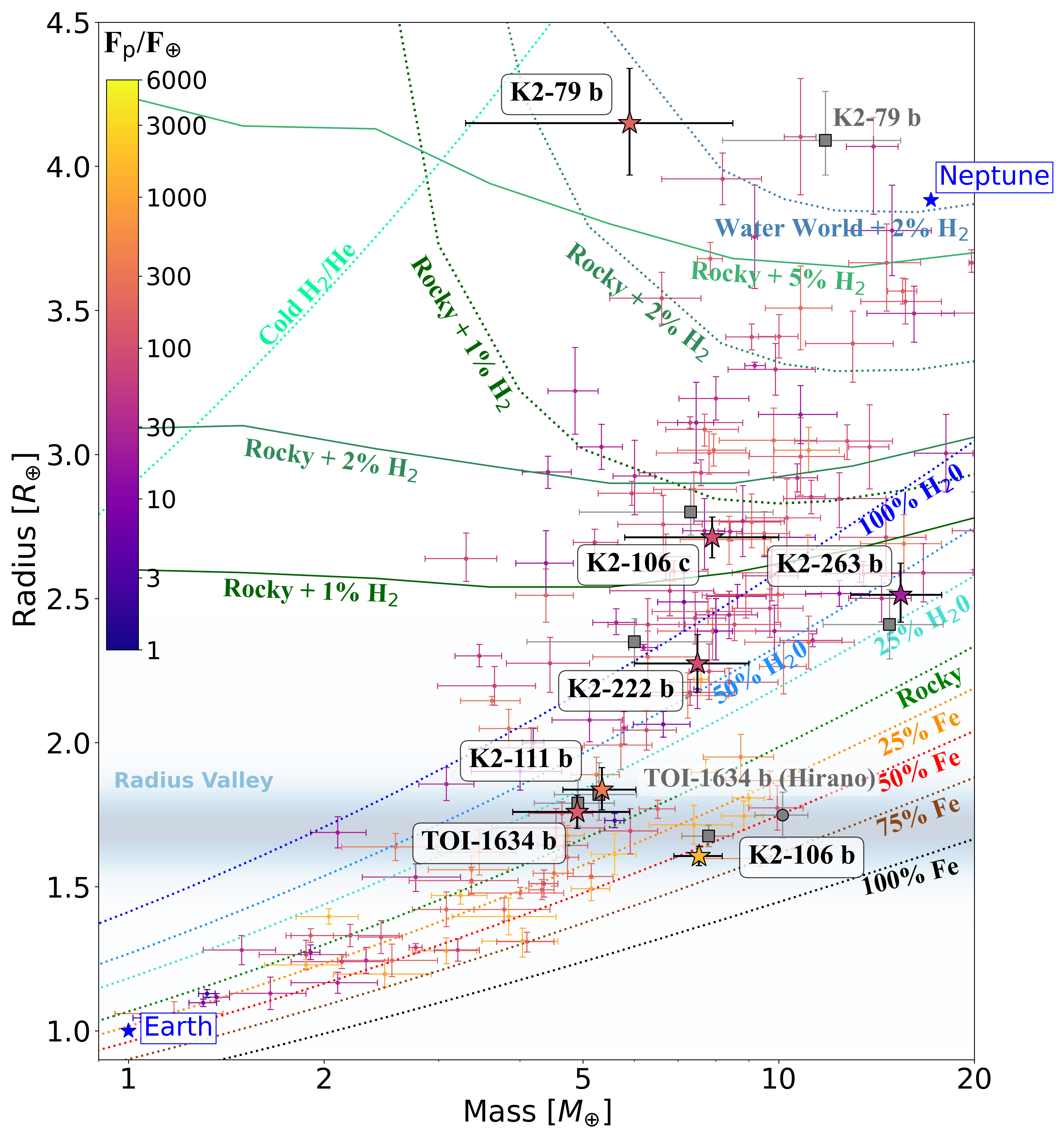
We place the mass and radius measurements of the transiting planets into context and compare them to composition models in Figure 7, which shows a mass-radius (M-R) plot for small planets ($R<4.5$ $R_{\oplus}$ and $M<$ 20 $M_{\oplus}$). Confirmed planets, with a mass and radius estimated to a precision better than 20% and 5%, respectively, taken from TepCat (Southworth, 2011) are also shown. Furthermore, the coloured lines in the M-R plot show different compositions, taken from Zeng et al. (2019) (dashed lines) and Lopez and Fortney (2014) (solid lines). We include both models for completeness, but note that the H/He relations from Zeng et al. (2019) are not appropriate for planets actively losing their atmospheres, as shown by Rogers et al. (2023). While the 1000 K Zeng et al. (2019) curves remain useful for illustrating the broader sample, for K2-106 c we adopt the Lopez and Fortney (2014) models as the default, since they assume a fixed system age and therefore better capture planets undergoing mass loss.

Figure 7: M–R diagram. Planet results from this study are shown as coloured stars, while archival literature values for the same planets (Table 1) appear as grey symbols with error bars; squares for most planets and a circle for the alternative TOI-1634 b value from Hirano et al. (2021). Other confirmed planets with mass and radius precisions better than 20% and 5%, taken from TepCat (Southworth, 2011), are also plotted. Dotted lines show compositions from Zeng et al. (2019) (1000 K), and solid lines from Lopez and Fortney (2014) (1 Gyr, solar metallicity, 1000 $F_{\oplus}$). Points are colour-coded by incident flux. Earth, Neptune, and the approximate radius valley (Fulton et al., 2017) are indicated. Archival points are not individually labelled; exceptions are K2-79 b and one of the TOI-1634 b measurement, where the closest grey point corresponds to the Cloutier et al. (2021) solution.

As a next step, we used the planetary properties derived from the combined transit and RV fits to model the internal structure of the transiting planets. This was done using the plaNETic framework (Egger et al., 2024), which uses a neural network trained on the BICEPS forward model (Haldemann et al., 2024) as a fast surrogate model in combination with a full grid accept-reject sampling scheme. Each planet is assumed to consist of a volatile layer (H, He, H₂O), a mantle layer (SiO₂, MgO, FeO) and an inner core (Fe, FeS).

There is a high degeneracy when inferring the internal structure of exoplanets based on their mean density alone. The resulting posterior distributions will therefore to some extent depend on the chosen priors. We run here six different models for each planet, combining different prior options for the planetary Si/Mg/Fe ratios with prior options for the envelope compositions. More specifically, explore three assumptions for the planetary Si/Mg/Fe ratios: (1) that they match those of the host star exactly (following e.g. Thiabaud et al., 2015); (2) that the planets are iron-enriched relative to their host star, using the empirical relation of Adibekyan et al. (2021); and (3) that the planetary Si/Mg/Fe ratios are allowed to vary freely, independent of the stellar abundances. In addition, we consider two possibilities for the volatile envelope: (A) a water-enriched composition, consistent with formation beyond the ice line, and (B) a primarily H/He-dominated envelope, consistent with formation inside the ice line. Further details on these priors can be found in Egger et al. (2024). The resulting constraints for the transiting planets studied here are summarised in the following.

4.1.1 K2-79 b

K2-79 b, with a measured mass of $M_{\rm b}=5.9\pm 2.6\,M_{\oplus}$ and radius of $R_{\rm b}=4.15_{-0.18}^{+0.19}\,R_{\oplus}$, lies well above the bulk of the small-planet population in Figure 7, occupying the low-density sub-Saturn regime. Its resulting bulk density of $\rho_{\rm b}\approx 0.45\mathrm{g\,cm^{-3}}$ indicates the presence of a substantial volatile-rich envelope. While Nava et al. (2022) reported a somewhat higher mass and slightly smaller radius, the updated parameters presented here place K2-79 b even father from rocky or water-world compositions, reinforcing its classification as a highly inflated low-mass planet.

Our interior modelling confirms that a wide range of compositions remain viable. Under water-rich priors (prior A), we infer envelope mass fractions spanning from a few per cent up to $\sim$ 60%, consistent with envelopes containing a broad range of water mass fractions. For the water-poor prior, the models favour H/He-dominated atmospheres with envelope mass fraction of $6^{+2}_{-3}$%, in agreement with expectations from formation and evolution scenarios for low-density sub-Saturns. Given the planet’s high irradiation ($F_{\rm b}\approx 180\,F_{\oplus}$) and low surface gravity ($g_{\rm b}\approx 0.34\,g_{\oplus}$), such an H/He envelope would be susceptible to long-term escape unless supported by heavier volatiles, whereas a water-rich composition naturally gives a more resilient atmosphere of Gyr timescales.

Transmission spectroscopy with the James Webb Space Telescope (JWST; Gardner et al., 2006) or the Atmospheric Remote-sensing Infrared Exoplanet Large-survey (Ariel; Tinetti et al., 2018) could help discriminate between these possibilities. A hydrogen-rich atmosphere is expected to produce spectral modulations of $\Delta d\sim$230–240 ppm over five scale heights, while a more water-enriched enveople would reduce the signal to $\sim$ 130 ppm, as also noted by Nava et al. (2022).

4.1.2 K2-106 b & c

K2-106 b, with a mass of $M_{\rm b}=7.54_{-0.64}^{+0.65}\,M_{\oplus}$ and radius $R_{\rm b}=1.606_{-0.033}^{+0.034}\,R_{\oplus}$, lies well inside the rocky region of the M–R diagram (Figure 7). Its bulk density of $\rho_{\rm b}\approx 9.3\,\mathrm{g\,cm^{-3}}$ places it among the densest known USP planets, overlapping with the compositional curves for rocky or iron-rich interiors. Although its position on the M–R diagram overlaps the rocky and iron-rich composition curves, this does not uniquely imply an Earth-like core-mantle fraction: such a structure is only permitted in our interior modelling if the mantle is enriched in iron relative to solar-composition silicates. Degeneracies in interior structure models (Hakim et al., 2018; Suissa et al., 2018) mean that a range of refractory compositions are possible, particularly given the extreme surface conditions expected for such a highly irradiated ($F_{\rm b}\approx 4620\,F_{\oplus}$ and short-period ($P_{\rm b}=0.57130782_{-0.00000057}^{+0.00000056}$ days) planet.

Our interior modelling further supports the interpretation of K2-106 b as a largely atmosphere-free core. In the water-poor case, reproducing the observed density requires envelope mass fractions below $10^{-6}$, far too small for a low-mean-molecular-weight (MMW) atmosphere to survive long-term photoevaporation. This strongly indicates that the planet is effectively a bare core. In the water-rich case, fixing the planetary Si/Mg/Fe ratios to stellar abundances fails to reproduce the observed density, consistent with Rodríguez Martínez et al. (2023), who argue that K2-106 b cannot simultaneously host a steam atmosphere and reflect the refractory abundances of its host star. Allowing the interior elemental ratios to vary does permit thin steam envelopes with mass fractions of $0.3^{+0.7}_{-0.2}$% and $0.4^{+0.8}_{-0.3}$% for priors A2 and A3, respectively. However, even these very small volatile layers may struggle to remain stable against hydrodynamic escape over Gyr timescales given the planet’s extreme irradiation. A more detailed atmospheric-loss calculation is beyond the scope of this work, but the plausibility of such long-lived steam envelopes should be approached with caution.

Despite its high density, K2-106 b could still host a transient or hybrid atmosphere generated by surface outgassing or a magma ocean (Ito et al., 2015; Bower et al., 2022). Such atmospheres would be dominated by heavy species (e.g. CO, SiO) and may be detectable through infrared spectroscopy or thermal phase-curve measurements with JWST or future high-resolution instruments such as the CRyogenic InfraRed Echelle Spectrograph Upgrade project (CRIRES+; Dorn et al., 2023).

K2-106 c has a similar mass to K2-106 b but a substantially larger radius ($R_{\rm b}=2.712\pm 0.071\,R_{\oplus}$), placing it above the radius valley and implying the presence of a significant volatile envelope. In the water-poor case, we infer tightly constrained H/He-dominated envelope mass fractions of $1.5\pm 0.3$%, $1.9\pm 0.5$%, and $1.8^{+0.7}_{-0.6}$% for priors B1, B2, and B3, respectively. In the water-rich scenario, a broad range of compositions remains possible. Its location on M–R diagram is compatible with either a sub-Neptune-like H/He envelope of $\sim$1-2% by mass (consistent with Lopez and Fortney (2014)) or a water-rich composition (Zeng et al., 2019).

K2-106 c receives a moderate flux ($F_{\rm b}\approx 70\,F_{\oplus}$), close to the empirical threshold where atmospheric escape becomes efficient over Gyr timescales (Lopez and Fortney, 2013; Owen and Wu, 2017; Fulton and Petigura, 2018). The contrasting atmospheric outcomes of planets b and c — nearly identical in mass yet markedly different in radius — are naturally explained by atmospheric loss mechanisms such as XUV-driven escape or core-powered mass loss (Lopez and Fortney, 2014; Ginzburg et al., 2018), similar to the interpretation proposed for other compact multi-planet systems spanning the radius valley, such as GJ 9827 (Rice et al., 2019).

Together, the K2-106 planets provide a valuable test case for models of atmospheric evolution: K2-106 b likely represents an exposed rocky core, while K2-106 c has retained a volatile envelope. Future observations with JWST or high-resolution spectroscopy will be crucial for distinguishing between H/He- and H₂O-rich scenarios for K2-106 c and for probing any residual atmosphere or surface vapour on K2-106 b.

4.1.3 K2-111 b

K2-111 b resides just above the radius valley and falls between the 50% H₂O and rocky composition curves in Figure 7. Its bulk density of $\rho_{\rm b}\approx 4.7\,\mathrm{g\,cm^{-3}}$ is lower than that of a iron-free rocky composition, indicating that K2-111 b cannot be explained as a bare silicate core and must retain at least modest volatile envelope. At the same time, its high incident flux ($F_{\rm b}\approx 490\,F_{\oplus}$) and likely old age imply that any long-lived atmosphere cannot be dominated by low-MMW species, which would be efficiently removed by photoevaporation. This places the planet in a particularly informative region of the M–R diagram: too dense to be a stripped rocky core, yet too irradiated to host a primordial H/He envelope.

Our interior modelling reflects this tension. For water-poor priors, we obtain extremely small envelope mass fractions of $10^{-6}-10^{-5}$, which would be rapidly lost to hydrodynamic escape and are therefore not viable long-term solutions. In contrast, the water-rich priors allow steam-dominated atmospheres with mass fractions of $10^{+8}_{-6}$%, $13^{+9}_{-7}$%, and $16^{+10}_{-9}$% for priors A1, A2, and A3. These heavier, higher-MMW envelopes are far more resistant to atmospheric escape, and their presence would naturally explain the observed density.

This interpretation is further supported by the chemical properties of the host star. K2-111 is iron-poor but $\alpha$-enhanced ([$\alpha$/Fe] = 0.27; Mortier et al., 2020), which can favour lower planetary core densities for a given mass (Santos et al., 2017). A steam-dominated envelope atop a composition influenced by the star’s non-solar refractory ratios therefore provides a consistent explanation for the planet’s bulk properties. The requirement for heavier volatiles closely parallels the case of TOI-238 b, where an evaporation analysis showed that a steam atmosphere can indeed remain stable over Gyr timescales despite high irradiation (Egger et al., 2025). A similar analysis for K2-111 b would likely confirm that a water-rich or mixed volatile envelope is able to survive long-term atmospheric escape, whereas a H/He-dominated envelope would not.

Taken together, these results suggest that K2-111 b is best described as a rocky planet that retains a significant steam-rich envelope shaped both by its host star’s chemistry and by strong atmospheric escape over its lifetime.

4.1.4 K2-222 b

K2-222 b lies above the radius valley in Figure 7, with a bulk density of $\rho_{\rm b}\approx 3.5\,\mathrm{g\,cm^{-3}}$, which is significantly lower than that of a purely rocky composition, indicating the presence of a volatile-rich envelope. Using the revised orbital parameters, we derive an incident flux of $F_{\rm b}\approx 67\,F_{\oplus}$, lower than the $\sim 95\,F_{\oplus}$ estimated by Nava et al. (2022). The discrepancy stems from differing luminosities: their value is model-derived, whereas ours is scaled from the measured stellar radius and effective temperature. The updated flux places K2-222 b closer to the regime where long-term atmospheric retention is plausible, though not guaranteed.

Our interior modelling allows both water-rich and water-poor solutions. Under the water-rich priors (prior A), we infer high-MMW envelopes with mass fractions $35^{+11}_{-15}$% and water mass fractions between 94–100%. These solutions correspond to planets with substantial steam-rich or mixed volatile atmospheres. In contrast, the water-poor priors result in very low-mass H/He-dominated envelopes with mass fractions of $0.2^{+0.2}_{-0.1}$%, $0.3^{+0.3}_{-0.2}$%, $0.3^{+0.4}_{-0.2}$% for priors B1–B3. Given K2-222 b’s high flux and moderate surface gravity ($g_{\rm b}\sim 1.44\,g_{\oplus}$), such extremely small H/He layers lie near the threshold of long-term stability and may be vulnerable to photoevaporation.

This places K2-222 b in a boundary region similar to K2-111 b: too large to be a bare rocky core, but potentially unable to retain a low-MMW atmosphere over Gyr timescales. If the tenuous H/He envelopes allowed by the water-poor priors are unstable, the planet would require a higher-MMW (e.g. steam-rich) envelope to survive to the present day. Such water-rich compositions also remain fully consistent with its mass and radius, as show by the Zeng et al. (2019) models.

4.1.5 K2-263 b

K2-263 b is a temperate, intermediate-mass planet whose updated properties reinforce its classification as a cold sub-Neptune with a mixed ice-rock interior with a bulk density of $\rho_{\rm b}\approx 3.5\,\mathrm{g\,cm^{-3}}$. On the M–R diagram, the planet lies between 25% and 50% H₂O composition curves, consistent with a substantial volatile or ice-rich interior. This is in line with the interpretation of Mortier et al. (2018), who suggested that K2-263 b likely contains comparable fractions of rocky and icy material, pointing to formation beyond the snow line followed by inward migration.

Our interior modelling supports this picture and allows both water-rich and water-poor envelope compositions. Under the water-rich priors (A1–A3), K2-263 b is compatible with steam-dominated envelopes with mass fractions of $25^{+12}_{-11}$%, $31^{+11}_{-14}$%, and $26^{+13}_{-12}$%. Such solutions correspond to high-MMW atmospheres overlaying a substantial ice-rock interior. Meanwhile, the water-poor priors (B1–B3) permit H/He-dominated envelopes with mass fractions of $0.6^{+0.5}_{-0.3}$%, $0.7^{+0.6}_{-0.5}$%, and $0.8^{+0.8}_{-0.6}$%. These thin, hydrogen-rich envelopes also reproduce the observed density due to the planet’s comparatively large solid interior.

With a long orbital period, low incident flux ($F_{\rm b}\sim 8.1\,F_{\oplus}$), and an equilibrium temperature of $T_{\rm eq,b}\approx 480$ K, K2-263 b occupies the cool end of the sub-Neptune population. It is comparable in mass and radius to Kepler-131 b (Marcy et al., 2014) and HD 106315 b (Barros et al., 2017; Crossfield et al., 2017), but stands out for its significantly lower irradiation and higher mean density. These characteristics make K2-263 b a valuable analogue for the predicted population of cold, water-rich super-Earths and an important benchmark for models of planet formation, migration, and volatile retention in the low irradiation regime above the radius valley. K2-263 b therefore joins the emerging population of sub-Neptunes with $T_{\rm eq}<600$ K that are likely to possess water-rich compositions around FGK dwarfs (e.g. the cold sub-Neptune candidates discussed in Bonomo et al. (2025)). This group remains sparsely sampled, and K2-263 b provides a valuable addition that helps anchor the low-irradiation end of the M-R distribution.

4.1.6 TOI-1634 b

TOI-1634 b occupies a compositionally intriguing region of the M–R diagram, lying just above the 100% silicate (iron-free) bare-core line and near the upper edge of the radius valley. With updated parameters, the planet has a bulk density of $\rho_{\rm b}\approx 4.9\,\mathrm{g\,cm}^{-3}$. This value is lower than that of a pure silicate composition, indicating that TOI-1634 b cannot be explained as a bare rocky core and must retain at least a small volatile component or a non-Earth-like refractory mixture. Given its intense isolation ($F_{\rm b}\approx 121\,F_{\oplus}$) and USP-like characteristics, TOI-1634 b occupies a transitional regime where atmospheric loss is expected to be strong, making it a key system for understanding the mechanisms that shape the radius valley.

Our interior modelling reflects this balance between density and evaporation. For the water-poor priors, we obtain extremely small H/He envelope mass fractions, which would be rapidly removed by photoevaporation and are therefore not viable long-term solutions. In contrast, the water-rich priors result in steam-dominated envelopes with mass fractions of $17^{+11}_{-9}$%, $12^{+10}_{-7}$%, and $22^{+11}_{-11}$% for priors A1–A3. These higher-MMW envelopes are far more stable against hydrodynamic escape and naturally account for the planet’s position above the pure-silicate line. As with K2-111 b, TOI-1634 b appears to lie in a regime where only heavier volatile envelopes — no primordial hydrogen — can survive over Gyr timescales.

These findings help place the planet within the broader context of previous work. Cloutier et al. (2021) suggested that an extended H/He envelope could explain the radius, but argued that such an atmosphere would be highly vulnerable to photoevaporation. Hirano et al. (2021), using IRD RVs, instead found a density consistent with a purely rocky interior. Overall, TOI-1634 b represents an important benchmark for understanding USP planets near the radius valley, highlighting the interplay between the composition, irradiation-driven atmospheric escape, and the requirement for higher-MMW volatiles to maintain even a thin envelope over the system’s lifetime.

4.2 Prospects for mission planning

An accurate knowledge of an exoplanet’s transit ephemeris is essential for planning future time-critical observations, for example Dragomir et al. (2020) showed that 81% of TESS planet ephemerides will have mid-transit uncertainties exceeding 30 min after just one year. For high-demand facilities, such as JWST and the upcoming Ariel and HWO, maintaining precise ephemerides is critical to avoid wasted observing time and ensure full transit coverage. For many transiting systems discovered by missions like Kepler and K2, formal uncertainties in orbital period and transit epoch propagate into substantial timing uncertainties when extrapolated into the mid-2040s, when HWO is due to launch (Ikwut-Ukwa et al., 2020). Without ephemeris updates, many promising targets will have transit windows too uncertain to schedule efficiently, without significant and time-critical re-analysis, which is often infeasible close to observation deadlines. In this study, we demonstrate that combining all published transit observations, especially with the addition of just two recent CHEOPS transits, for a given planet can significantly reduce these uncertainties, in many cases restoring sub-hour precision at the expected launch of HWO (assumed here as $\sim$ BJD 2467981.50, i.e. $\sim$2045).

Table 6: Summary of improvements in transit ephemerides for all transiting planets in this sample. Columns show the original, TESS-updated, and TESS+CHEOPS-updated period uncertainties ($P_{\rm err}$) and corresponding transit time uncertainties ($T_{0,{\rm err}}$) propagated to 2045 January 01 (BJD 2467981.50). The factors $\sigma P$ and $\sigma T$ quantify the improvement relative to the preceding fit stage, and the final three columns list the ROP (return on precision), defined as seconds of uncertainty reduced per hour of new observing time for TESS, CHEOPS, and the combined dataset, respectively.

Planet	$P_{\rm err}$ [s]	$P_{\rm err}$ [s]	$P_{\rm err}$ [s]	$\sigma P_{TESS}$	$\sigma P_{CHEOPS}$	$T_{0_{\rm err}}$ [hr]	$T_{0_{\rm err}}$ [hr]	$T_{0_{\rm err}}$ [hr]	$\sigma T_{TESS}$	$\sigma T_{CHEOPS}$	ROPTESS	ROPCHEOPS	ROPtotal
	(Literature)	(+TESS)	(+CHEOPS)			(Literature)	(+TESS)	(+CHEOPS)			[$\mathrm{s\,hr}^{-1}$]	[$\mathrm{s\,hr}^{-1}$]	[$\mathrm{s\,hr}^{-1}$]
K2-79 b	33.70	2.89	1.25	11.64	2.31	9.26	0.62	0.27	14.87	2.31	12.00	66.42	12.40
K2-106 b	0.48	0.05	0.05	9.65	1.07	2.45	0.21	0.20	11.69	1.07	6.21	2.06	6.14
K2-106 c	59.62	59.62	1.81	1.00	40.00	13.13	13.13	0.33	1.00	40.03	0.0	1470.89	34.71
K2-111 b	34.56	0.90	0.90	38.28	1.00	19.52	0.41	0.41	47.45	1.00	53.08	0.00	51.74
K2-222 b	76.03	1.08	0.90	70.40	1.20	14.52	0.17	0.14	86.12	1.21	26.58	5.72	26.39
K2-263 b	8.12	9.50	5.79	0.85	1.64	0.44	0.45	0.27	0.98	1.64	-0.01	24.51	0.23
TOI-1634 b†	1.30	0.04	0.03	37.50	1.10	3.34	0.08	0.07	40.94	1.10	9.06	0.20	8.27
Note: † TOI-1634 b was initially validated with TESS and ground-based photometry rather than K2; the second column corresponds to the improvement from an additional TESS sector, and the third column includes the final CHEOPS observations.

Figure 8: Projected absolute transit time uncertainties ($T_{\mathit{0},\,err}$) at the 2045 epoch for the seven transiting planets analysed in this study. Each bar represents the 1$\sigma$ timing window centred on the nominal transit mid-time. Light red bars correspond to the original transit ephemerides published in the literature (source papers referenced in Table 1), yellow bars show the improvement obtained after adding the TESS transits, and the dark red bars indicate the final precision after including CHEOPS observations.

We analysed seven transiting planets with archival and new photometry spanning K2, TESS, CHEOPS, and other ground-based sources, producing updated ephemerides via a global fit of all available transit times. For each planet, three sequential fits were performed: (1) using the original discovery data only, (2) adding TESS transits, and (3) subsequently adding CHEOPS transits. This stepwise approach isolates the specific contribution of each mission to the final precision achieved. The resulting improvements are shown in Figure 8, which presents the absolute transit time uncertainties in hours for each planet in $\sim$ 2045, comparing the original predictions (source papers referenced in Table 1) with the ones from this study.

To estimate the projected transit time uncertainty at that epoch, we use:

$$\sigma_{T}=\sqrt{\sigma_{T_{0}}^{2}+(N\cdot\sigma_{P})^{2}}$$ (1)

where $\sigma_{T_{0}}$ corresponds to the error on the transit centre time, $\sigma_{P}$ corresponds to the error on the orbital period, and $N$ is the number of orbits between the reported transit centre time and the 2045 epoch (calculated as $N=(T_{2045}-T_{0})/P$).

To quantify the efficiency of these ephemeris refinements, we also introduce a metric for return on precision (ROP), defined as the number of seconds of future timing uncertainty reduced per hour of new observing time:

$$\text{ROP}\,[\mathrm{s\,hr}^{-1}]=3600\times\frac{T_{0_{\rm err,\,1}}-T_{0_{\rm err,\,2}}}{t_{\rm obs}}$$ (2)

where $T_{0_{\rm err,\,1}}$ and $T_{0_{\rm err,\,2}}$ are the predicted transit time uncertainties before and after the addition of new observations, respectively, and $t_{\rm obs}$ is the total duration in hours of the new observing data included in that stage. We computed three related quantities: (1) ROP_TESS — the improvement achieved by adding TESS data relative to the original literature ephemeris, (2) ROP_CHEOPS — the improvement achieved by subsequently adding CHEOPS data relative to the TESS-only fit, and (3) ROP_total — the cumulative improvement from both missions combined. This formulation allows the relative contributions of each mission to be separated, while still expressing their combined impact on long-term predictability. Both missions extend the temporal baseline and provide additional transits that constrain $P$ and $T_{0}$. More recent observations from CHEOPS are particularly valuable for this reason, while TESS often provides the dominant improvement for systems where multiple transits were observed per sector. A full numerical summary of the results is provided in Table 6.

Planets with relatively long orbital periods or limited early baselines benefited the most from these multi-mission ephemeris refinements, as their timing uncertainties grow fastest when extrapolated into the future. For example, K2-222 b originally had a predicted uncertainty of $\sim$ 14.5 hours in 2045, which improved by a factor of $\sim$ 70$\times$ after including TESS data alone, and by a further $\sim$ 1.2$\times$ once the new CHEOPS transits were added. This corresponds to an overall ROP of 26.39 $\mathrm{s\,hr}^{-1}$, meaning that for every hour of new observing time from TESS and CHEOPS combined, $\sim$ 26 seconds of future scheduling are recovered — amounting to just over 14 hours saved in total. K2-79 b showed a similar trend, improving by $\sim$ 12$\times$ after adding TESS and then an additional $\sim$ 2.3$\times$ after incorporating the CHEOPS transits, highlighting the cumulative impact of combining wide-field survey data with targeted follow-up. For K2-263 b, only a single TESS transit was detected across four sectors due to its 50.8-day period. The limited coverage and lower timing precision led to a slight degradation in the ephemeris relative to the K2-only solution. The addition of two high-quality CHEOPS transits, however, recovered and modestly improved the overall precision, yielding a new $\sim$ 1.6$\times$ gain. Given the planet’s extensive prior K2 coverage (one long-cadence and two short-cadence campaigns) the projected timing uncertainty by 2045 was already small, so the absolute improvement time remains marginal. This case illustrates how, for well-constrained long-period systems, CHEOPS can refine ephemerides where TESS contributes little due to sparse transit sampling. K2-106 b was already published with one TESS sector (Guenther et al., 2024), so the addition of a single new TESS sector only modestly improved the precision (period uncertainty improved by $\sim$ 9.7$\times$, and the projected 2045 timing uncertainty decreased from $\sim$ 2.45 hours to $\sim$ 0.21 hours). In contrast, K2-106 c saw no improvement from the TESS data, as all transits fell within sector data gaps; the full $\sim$ 40$\times$ enhancement in period precision arises directly from the dedicated CHEOPS visits. This clearly demonstrates the importance of dedicated follow-up even for targets nominally covered by wide-field surveys. This stepwise comparison illustrates that while TESS generally provides the largest single boost to ephemeris precision, CHEOPS plays a critical role in maintaining and restoring sub-hour predictability for targets otherwise missed or poorly sampled by TESS.

Without updated ephemerides, these targets would have been unsuitable for transmission spectroscopy, high-contrast imaging, or precision scheduling in the extrapolated future — such as when HWO is expected to be operational. K2-111 b, whose projected timing uncertainty at the launch of the HWO era was $\sim$ 20 hours based on its original K2-only ephemeris, would have posed a significant challenge for precise scheduling. By incorporating all available data, this was reduced to just $\sim$ 0.41 hours (a $\sim$ 47$\sigma$ improvement). This corresponds to an ROP_total of 52 $\mathrm{s\,hr}^{-1}$, meaning that each hour of follow-up observation recovered roughly 52 seconds of future scheduling uncertainty. Although the gain per hour is modest due to the large cumulative observing due to TESS, the overall 19-hour reduction in projected uncertainty makes the planet far more viable for time-critical follow-up during the HWO era. For TOI-1634 b, which was initially validated using TESS and ground-based photometry, adding one additional TESS sector modestly reduced the projected 2045 timing uncertainty, and the CHEOPS observations further improved it by $\sim$ 12%. This demonstrates that even recently discovered systems benefit from regular ephemeris maintenance to maintain sub-hour predictability over multi-decade baselines, particularly as TESS is expected to cease Northern Hemisphere observations in the near future. As shown in Figure 8, the improvements in orbital period uncertainty ($\sigma_{P}$) directly translate into long-term gains, since timing error increases linearly with time due to $N\sigma_{P}$ accumulation across orbits. Overall, the updated period uncertainties in this study are typically reduced by roughly an order of magnitude or more compared to previously published values, with the largest gains occurring for systems with sparse initial coverage or long orbital periods, and smaller but still measurable improvements for planets with long baselines or previously precise ephemerides.

In addition to this, several of the systems we examined also host non-transiting outer planets identified via RV measurements: K2-111 c and K2-222 c. These companions orbit at periods approximately 3–10$\times$ longer than their transiting counterparts and may induce subtle dynamical perturbations, such as TTVs or long-term precession. In this analysis, no significant TTVs were detected, and the observed CHEOPS transits occur at the epochs predicted by the extrapolated ephemerides. This indicates that any dynamical effects are either negligible or not detectable with the current data. More broadly, systems with known but non-transiting companions present an additional motivation for maintaining accurate ephemerides. In such cases, the transiting planet may be the only directly observable tracer of the system’s architecture. Ensuring that its future transits are precisely predictable not only enables atmospheric characterisation but also preserves the possibility of detecting long-term dynamical perturbations, which may be caused by additional, non-transiting planets in the system. These effects, often undetectable in sparse datasets, can accumulate over time and introduce deviations from linear ephemerides. Thus, ephemeris precision plays a foundational role in enabling follow-up science in multi-planet systems, whether or not all planets are seen in transit.

5 Conclusions

These results underscore the importance of routine ephemeris updates, especially for high-priority targets with long orbital periods or sparse follow-up coverage. As the exoplanet community prepares for missions with increasingly demanding scheduling constraints, such as HWO and Ariel, the timely maintenance of accurate ephemerides will be essential to ensure that observing opportunities are not lost. This work demonstrates a straightforward and scalable approach to doing so, using publicly available photometry and accessible fitting tools to combine archival and recent transit timings.

When considering the relative contributions of TESS and CHEOPS, both missions play distinct but complementary roles in maintaining precise transit ephemerides. For most systems, TESS delivered the largest improvement by extending the temporal baseline and adding multiple new transits, typically reducing the projected 2045 timing uncertainties by an order of magnitude or more relative to the original K2 fits. The subsequent CHEOPS observations — 151 hours across six of the AO-2 targets (excluding TOI-1634 b as the DDT skews the sample) — provided a further cumulative reduction of about 61 hours in predicted timing uncertainty. These AO-2 systems exhibit a mean ROP of $\sim$ 21 $\mathrm{s\,hr^{-1}}$, corresponding to roughly 21 seconds of future scheduling precision recovered per hour. While this per-hour figure may appear modest, these small gains compound significantly over multi-decade baselines, translating into many hours of improved transit predictability by the 2040s. Together, TESS and CHEOPS demonstrate how combining broad-survey coverage with targeted, high-cadence follow-up can restore sub-hour predictability for established systems, safeguarding them for future atmospheric and dynamical studies with future facilities.

Beyond refined ephemerides, this analysis provides significantly improved planetary parameters for seven small transiting planets, resulting in more precise masses, radii, and bulk densities. These worlds span a wide compositional range: from the dense, rocky or iron-rich interior of K2-106 b to the moderately dense, steam-rich or higher-MMW envelopes inferred for TOI-1634 b and K2-111 b, and the volatile-rich or mixed rock-ice compositions of K2-263 b and K2-79 b. Their diversity emphasises the complexity of small planet formation and the importance of well-constrained M–R relationships for testing models of atmospheric loss and interior structure. Several of these systems also host non-transiting companions inferred from long-term RV trends — such as K2-111 c and K2-222 c — which may play an important role in shaping the dynamical evolution and composition of their inner planets. Continued RV monitoring will be crucial for fully resolving these outer companions and characterising their impact on system architecture.

Overall, this work illustrated the lasting value of coordinated photometric and spectroscopic follow-up. The combination of CHEOPS transits, HARPS-N RVs, and archival K2, TESS, and ground-based data has produced ephemerides precise enough to enable atmospheric and interior studies well into the 2040s. As future characterisation missions target cooler and smaller exoplanets, reliable ephemerides and accurate physical parameters will be essential foundations. Sustained investment in precision follow-up — particularly for legacy systems discovered a decade or more ago — remains essential to building a statistically robust population of small exoplanets and maximising the scientific return of upcoming missions.

Data Availability

This paper includes raw data collected by the K2 mission, which are publicly available from MAST (https://archive.stsci.edu/missions-and-data/k2). Raw data collected by the TESS mission are also publicly available from MAST (https://archive.stsci.edu/tess). Raw data collected by CHEOPS can be found using the file keys in Table 8 at https://cheops-archive.astro.unige.ch/archive_browser/. Observations made with HARPS-N on the Telescopio Nazionale Galileo 3.6 m telescope are available at the CDS (https://cds.unistra.fr).

Appendix A Photometric Observations Summary

Table 7: Summary of K2 and TESS Observations.

Target	Campaign / Sector	Program IDs
K2-79	C4	GO4060 LC, GO4029 LC, GO4033 LC, GO4007 LC
K2-79	Sectors 42–44	G04205, G04242, G04223
K2-79	Sectors 70–71	G06165, G06058
K2-106	C8	GO8068 LC, GO8032 LC, GO8077 LC
K2-106	Sector 42	G04205, G04242, G04223
K2-106	Sector 70	G06165, G06058
K2-111	C4	GO4060 LC, GO4033 LC, GO4007 LC
K2-111	Sectors 70-71	Mission-selected target (no GI ID)
K2-222	C8	GO8068 LC, GO8051 LC, GO8032 LC, GO8077 LC
K2-222	Sectors 42-43	G04205, G04059, G04242, G04191, G04223
K2-222	Sector 70	G06165, G06200, G06058
K2-263	C5	GO5007 LC, GO5029 LC, GO5033 LC, GO5104 LC, GO5106 LC, and GO5060 LC
K2-263	C16	GO16009 LC & SC, GO16011 LC, GO16015 LC & SC, GO16020 LC, GO16021 LC, GO16101 LC & SC
K2-263	C18	GO18027 LC & SC, GO18048 LC, GO18049 LC, GO18065 LC & SC, GO18901 LC
K2-263	Sector 44	G04231, G04205, G04242
K2-263	Sectors 45-46, 72	G06058
TOI-1634	Sector 18	G022198
TOI-1634	Sector 86	G07157, G07066

Table 8: Log of CHEOPS observations. The column T_exp gives the exposure time in terms of the integration time per image multiplied by the number of images stacked on-board prior to download. N_obs is the number of frames. Effic. is the proportion of the time in which unobstructed observations of the target occurred. R_ap is the aperture radius used for the photometric extraction. RMS is the standard deviation of the residuals from the best fit. The variables in the final column are as follows: time, t; spacecraft roll angle, $\phi$, PSF centroid position, (x, y); smear correction, smear; aperture contamination, contam; image background level, bg.

Target	Start date	Duration	Texp	Nobs	Effic.	File key	APER	Rap	RMS	Decorrelation
	(UTC)	(h)	(s)		(%)			(pixels)	(ppm)
K2-106 b	2021-09-17T00:49:50	11.61	1 x 60.0	560	80.3	CH_PR220007_TG000101_V0300	DEFAULT	25	18297	sin($\phi$), cos($\phi$), bg, contam, smear
K2-106 b	2021-09-20T10:47:56	11.61	1 x 60.0	560	80.3	CH_PR220007_TG000102_V0300	DEFAULT	25	17837	sin($\phi$), cos($\phi$), bg, contam, smear
K2-106 c	2021-09-15T19:31:53	15.72	1 x 60.0	755	79.9	CH_PR220007_TG000201_V0300	DEFAULT	25	10514	sin($\phi$), cos($\phi$), bg, contam, smear
K2-106 c	2021-09-29T04:02:52	15.72	1 x 60.0	638	67.6	CH_PR220007_TG000202_V0300	DEFAULT	25	7758	sin($\phi$), cos($\phi$), bg, contam, smear
K2-222 b	2021-10-04T05:02:00	8.84	1 x 60.0	366	68.9	CH_PR220007_TG000301_V0300	DEFAULT	25	567	No decorrelation needed.
K2-222 b	2021-11-03T23:42:00	9.22	1 x 60.0	375	67.7	CH_PR220007_TG000302_V0300	DEFAULT	25	1094	sin($2\phi$), cos($2\phi$)
K2-79 b	2021-12-06T08:12:52	8.39	1 x 60.0	312	61.9	CH_PR220007_TG000401_V0300	DEFAULT	25	34339	sin($\phi$), cos($\phi$), bg, contam, smear, t2, x2, y2,
										sin(2$\phi$), cos(2$\phi$)
TOI-1634 b	2021-11-07T21:20:51	10.69	1 x 60.0	391	60.9	CH_PR220007_TG000501_V0300	DEFAULT	25	1928	sin($\phi$), cos($\phi$), bg, contam, smear
TOI-1634 b	2021-12-18T11:04:54	11.36	1 x 60.0	363	53.2	CH_PR220007_TG000502_V0300	DEFAULT	25	18585	t, x, y, sin($\phi$), cos($\phi$), bg
K2-111 b	2021-10-15T05:39:50	16.66	1 x 60.0	547	54.7	CH_PR220007_TG000601_V0300	DEFAULT	25	2979	sin($\phi$), cos($\phi$), bg, contam, smear, t2, x2, y2,
										sin(2$\phi$), cos(2$\phi$)
K2-111 b	2021-10-31T07:04:52	16.84	1 x 60.0	602	59.5	CH_PR220007_TG000602_V0300	DEFAULT	25	13916	y, sin($\phi$), cos($\phi$), bg, contam, smear
K2-263 b	2022-01-05T04:36:52	12.41	1 x 60.0	432	58	CH_PR220007_TG000901_V0300	DEFAULT	25	10306	No decorrelation needed.
K2-263 b	2022-12-26T19:47:00	13.26	1 x 60.0	431	54.1	CH_PR220007_TG001501_V0300	DEFAULT	25	1246	t, x, y, sin($\phi$), cos($\phi$), bg
K2-79 b	2022-12-04T03:56:00	10.74	1 x 60.0	411	63.7	CH_PR220007_TG001601_V0300	DEFAULT	25	13256	t, x, y, sin($\phi$), cos($\phi$), bg
TOI-1634	2022-12-15T01:18:54	65.08	1 x 60.0	2202	56.4	CH_PR430015_TG000101_V0300	DEFAULT	25	2223	t, x, y, sin($\phi$), cos($\phi$), bg, contam, smear, t2,
(DDT)										x2, y2, sin(2$\phi$), cos(2$\phi$)
TOI-1634	2022-12-18T19:13:54	40.87	1 x 60.0	1331	54.3	CH_PR430015_TG000301_V0300	DEFAULT	25	2210	sin($\phi$), cos($\phi$), contam, smear, t2, x2, y2,
(DDT)										sin(2$\phi$), cos(2$\phi$)

Appendix B Joint Fits Figures

Figure 9: Combined fit results for K2-79 b. Transit fit to the light curve data from K2 long cadence (first row left), TESS long cadence (first row centre), and CHEOPS (first row right). The cadence (29.4 min for K2 long cadence, 120 s for TESS long cadence, and 60 s for CHEOPS) fluxes are plotted in grey, the fluxes binned every 30 min are over-plotted in black, and the fitted transit is shown by the red solid line. The RV fit to the HARPS-N & HIRES RVs is shown in the second row for K2-79 b. Coloured circular points show the phase folded RVs, grey points show these same values in subsequent phases, and the black line shows the best fit Keplerian model. The third row shows the RVs over the full $\sim 9$ yr baseline, illustrating the absence of any significant long term trend.

Figure 10: Combined fit results for K2-106 b. Transit fit to the light curve data from K2 long cadence (first row left), TESS long cadence (first row centre), TESS short cadence (first row right), and CHEOPS (second row left). The cadence (29.4 min for K2 long cadence, 120 s for TESS long cadence, 20 s for TESS short cadence, and 60 s for CHEOPS) fluxes are plotted in grey, the fluxes binned every 30 min are over-plotted in black, and the fitted transit is shown by the red solid line. The RV fit to the HARPS-N, HIRES, ESPRESSO, FIES, HARPS, HDS, and PFS RVs are shown in the second row right for K2-106 b. Coloured circular points show the phase folded RVs, grey points show these same values in subsequent phases, and the black line shows the best fit Keplerian model. The third row shows the RVs over the full $\sim 4$ yr baseline.

Figure 11: Combined fit results for K2-106 c. Transit fit to the light curve data from K2 long cadence (left) and CHEOPS (centre). The cadence (29.4 min for K2 long cadence and 60 s for CHEOPS) fluxes are plotted in grey, the fluxes binned every 30 min are over-plotted in black, and the fitted transit is shown by the red solid line. The RV fit to the HARPS-N, HIRES, ESPRESSO, FIES, HARPS, HDS, and PFS RVs are shown in the right for K2-106 c. Coloured circular points show the phase folded RVs, grey points show these same values in subsequent phases, and the black line shows the best fit Keplerian model.

Figure 12: Combined fit results for K2-111 b and RV fit results of K2-111 c. Transit fit to the light curve data from K2 long cadence (first row left), TESS long cadence (first row centre), and CHEOPS (first row right). The cadence (29.4 min for K2, 120 s for TESS, and 60 s for CHEOPS) fluxes are plotted in grey, the fluxes binned every 30 min are over-plotted in black, and the fitted transit is shown by the red solid line. The RV fit to the HARPS-N, HIRES, ESPRESSO, & FIES RVS are shown in the second row left for K2-111 b and second row right for K2-111 c. Coloured circular points show the phase folded RVs, grey points show these same values in subsequent phases, and the black line shows the best fit Keplerian model. The third row shows the RVs over the full $\sim 4$ yr baseline.

Figure 13: Combined fit results for K2-222 b and RV fit results of K2-222 c. Transit fit to the light curve data from K2 long cadence (first row left), TESS long cadence (first row centre), TESS short cadence (first row right), and CHEOPS (second row left). The cadence (29.4 min for K2 long cadence, 120 s for TESS long cadence, 20 s for TESS short cadence, and 60 s for CHEOPS) fluxes are plotted in grey, the fluxes binned every 30 min are over-plotted in black, and the fitted transit is shown by the red solid line. The RV fit to the HARPS-N & HIRES RVs are shown in the second row centre for K2-222 b and second row right for K2-222 c. Coloured circular points show the phase folded RVs, grey points show the values in subsequent phases, black line shows the best fit Keplerian model. The third row shows the RVs over the full $\sim 7$ yr baseline.

Figure 14: Combined fit results for K2-263 b. Transit fit to the light curve data from K2 long cadence (first row left), K2 short cadence (first row centre), TESS long cadence (first row right), and CHEOPS (second row left). The short cadence (29.4 min for K2 long cadence, 60 s for K2 short cadence, 120 s for TESS long cadence, and 60 s for CHEOPS) fluxes are plotted in grey, the fluxes binned every 30 min are over-plotted in black, and the fitted transit is shown by the red solid line. The RV fit to the HARPS-N RVs is shown in the second row right for K2-263 b. Coloured circular points show the phase folded RVs, grey points show these same values in subsequent phases, and the black line shows the best fit Keplerian model. The third row show the HARPS-N RVs over the full $\sim 4$ yr baseline.

Figure 15: RV results for TOI-1634. The top left panel shows the phase-folded HARPS-N RVs of the confirmed planet TOI-1634 b, with the best-fitting Keplerian model overplotted. The top right panel shows the HARPS-N RVs after subtraction of the signal of TOI-1634 b, folded at the characteristic period ($P\sim 100$ d) of a low-frequency modulation. The overplotted Keplerian curve in this panel is shown for illustrative purposes only and does not represent a confirmed planetary detection. Blue circular points show the phase-folded RVs, grey points show the same measurements repeated over multiple phases, and the black line indicates the corresponding model. The bottom panel shows the HARPS-N and IRD RVs as a function of time over the full $\sim$7 month baseline, highlighting the presence of additional low-frequency variability beyond the signal of TOI-1634 b.

Figure 16: Transit fit results for TOI-1634 b. Transit fit to the light curve data from TESS long cadence (first row left), TESS short cadence (first row centre), CHEOPS DDT (first row left), CHEOPS (second row left), OAA long cadence (second row centre), OAA short cadence (second row right), MuSCAT2 $g$-band (third row left), MuSCAT2 $r$-band (third row centre), MuSCAT2 $i$-band (third row right), MuSCAT2 $z_{s}$-band (fourth row left), LCOGT (fourth row centre), and RCO (fourth row right). The short/long cadence (120 s for TESS long cadence, 20 s for TESS short cadence, 60 s for CHEOPS, 120 s for OAA long cadence, 100 s for OAA short cadence, 40 s for LCOGT, 90 s for RCO, 46 s for MuSCAT2 $g$-band, 21 s for MuSCAT2 $i$- and $r$-bands, and 11 s for MuSCAT2 $z_{s}$-band) fluxes are plotted in grey, the fluxes binned every 30 min are over-plotted in black, and the fitted transit is shown by the red solid line.

References

- Ultra-short-period Planets in K2 with Companions: A Double Transiting System for EPIC 220674823. AJ 153 (2), pp. 82. External Links: Document, 1611.00397 Cited by: §3.2.
- A compositional link between rocky exoplanets and their host stars. Science 374 (6565), pp. 330–332. External Links: Document, 2102.12444 Cited by: §4.1.
- The HARPS-TERRA Project. I. Description of the Algorithms, Performance, and New Measurements on a Few Remarkable Stars Observed by HARPS. ApJS 200 (2), pp. 15. External Links: Document, 1202.2570 Cited by: §2.2.1.
- Magnetic activity in the HARPS M dwarf sample. The rotation-activity relationship for very low-mass stars through R’HK. A&A 600, pp. A13. External Links: Document, 1610.09007 Cited by: §2.2.1.
- Exploring the Effects of Stellar Magnetism on the Potential Habitability of Exoplanets. ApJ 969 (2), pp. 147. External Links: Document Cited by: §1.
- Precise masses for the transiting planetary system HD 106315 with HARPS. A&A 608, pp. A25. External Links: Document, 1709.00865 Cited by: §4.1.5.
- The Precision of Mass Measurements Required for Robust Atmospheric Characterization of Transiting Exoplanets. ApJ 885 (1), pp. L25. External Links: Document, 1910.00076 Cited by: §1.
- The Nature and Origins of Sub-Neptune Size Planets. Journal of Geophysical Research (Planets) 126 (1), pp. e06639. External Links: Document, 2010.11867 Cited by: §1.
- The CHEOPS mission. Experimental Astronomy 51 (1), pp. 109–151. External Links: Document, 2009.11633 Cited by: §1, §2.1.3.
- Dry or water world? How the water contents of inner sub-Neptunes constrain giant planet formation and the location of the water ice line. A&A 649, pp. L5. External Links: Document, 2104.11631 Cited by: §1.
- Disentangling between stellar activity and planetary signals. A&A 528, pp. A4. External Links: Document Cited by: §3.6.
- CHEOPS observations of the HD 108236 planetary system: a fifth planet, improved ephemerides, and planetary radii. A&A 646, pp. A157. External Links: Document, 2101.00663 Cited by: §2.1.3.
- In-depth characterization of the Kepler-10 three-planet system with HARPS-N radial velocities and Kepler transit timing variations. A&A 696, pp. A233. External Links: Document, 2502.07996 Cited by: §3.1, §4.1.5.
- Cold Jupiters and improved masses in 38 Kepler and K2 small planet systems from 3661 HARPS-N radial velocities. No excess of cold Jupiters in small planet systems. A&A 677, pp. A33. External Links: Document, 2304.05773 Cited by: §1, §3.1, §3.1, §3.2, §3.3, §3.4, §3.4, §3.5.
- Kepler Planet-Detection Mission: Introduction and First Results. Science 327 (5968), pp. 977. External Links: Document Cited by: §2.1.1.
- The exoplanet characterization toolkit (exoctk). Zenodo. External Links: Document, Link Cited by: §3.
- Retention of Water in Terrestrial Magma Oceans and Carbon-rich Early Atmospheres. \psj 3 (4), pp. 93. External Links: Document, 2110.08029 Cited by: §4.1.2.
- PIPE: Extracting PSF photometry from CHEOPS data. Note: Astrophysics Source Code Library, record ascl:2404.002 External Links: 2404.002 Cited by: §2.1.3.
- Las Cumbres Observatory Global Telescope Network. PASP 125 (931), pp. 1031. External Links: Document, 1305.2437 Cited by: §2.1.5.
- Attaining Doppler Precision of 3 M s-1. PASP 108, pp. 500. External Links: Document Cited by: §2.2.8.
- The NASA Exoplanet Archive and Exoplanet Follow-up Observing Program: Data, Tools, and Usage. \psj 6 (8), pp. 186. External Links: Document, 2506.03299 Cited by: §1.
- Limb and gravity-darkening coefficients for the TESS satellite at several metallicities, surface gravities, and microturbulent velocities. A&A 600, pp. A30. External Links: Document, 1804.10295 Cited by: §3.
- Limb and Gravity-darkening Coefficients for the Space Mission CHEOPS. Research Notes of the American Astronomical Society 5 (1), pp. 13. External Links: Document Cited by: §3.
- A new method to compute limb-darkening coefficients for stellar atmosphere models with spherical symmetry: the space missions TESS, Kepler, CoRoT, and MOST. A&A 618, pp. A20. External Links: Document, 1804.10135 Cited by: §3.
- TOI-1634 b: An Ultra-short-period Keystone Planet Sitting inside the M-dwarf Radius Valley. AJ 162 (2), pp. 79. External Links: Document, 2103.12790 Cited by: Table 1, Table 1, §2.1.5, §2.1.5, §2.1.5, §2.1.5, §2.2.1, §3.6, §3.6, Figure 7, §4.1.6.
- AstroImageJ: Image Processing and Photometric Extraction for Ultra-precise Astronomical Light Curves. AJ 153 (2), pp. 77. External Links: Document, 1701.04817 Cited by: §2.1.5.
- TESS Follow-up Observing Program Working Group (TFOP WG) Sub Group 1 (SG1): Ground-based Time-series Photometry. In AAS Meeting Abstracts #233, pp. 140.05. Cited by: §2.1.5.
- Harps-N: the new planet hunter at TNG. In Ground-based and Airborne Instrumentation for Astronomy IV, I. S. McLean, S. K. Ramsay, and H. Takami (Eds.), Society of Photo-Optical Instrumentation Engineers (SPIE) Conference Series, Vol. 8446, pp. 84461V. External Links: Document Cited by: §2.2.1.
- The Carnegie Planet Finder Spectrograph: integration and commissioning. In Ground-based and Airborne Instrumentation for Astronomy III, I. S. McLean, S. K. Ramsay, and H. Takami (Eds.), Society of Photo-Optical Instrumentation Engineers (SPIE) Conference Series, Vol. 7735, pp. 773553. External Links: Document Cited by: §2.2.8.
- The Carnegie Planet Finder Spectrograph: a status report. In Ground-based and Airborne Instrumentation for Astronomy II, I. S. McLean and M. M. Casali (Eds.), Society of Photo-Optical Instrumentation Engineers (SPIE) Conference Series, Vol. 7014, pp. 701479. External Links: Document Cited by: §2.2.8.
- The Carnegie Planet Finder Spectrograph. In Ground-based and Airborne Instrumentation for Astronomy, I. S. McLean and M. Iye (Eds.), Society of Photo-Optical Instrumentation Engineers (SPIE) Conference Series, Vol. 6269, pp. 626931. External Links: Document Cited by: §2.2.8.
- Two Small Transiting Planets and a Possible Third Body Orbiting HD 106315. AJ 153 (6), pp. 255. External Links: Document, 1701.03811 Cited by: §4.1.5.
- Effects of planetary mass uncertainties on the interpretation of the reflectance spectra of earth-like exoplanets. External Links: 2502.01513, Link Cited by: §1.
- Gliese 12 b, a temperate earth-sized planet at 12 parsecs discovered with tess and cheops. MNRAS 531 (1), pp. 1276–1293. External Links: Document, 2405.13118 Cited by: §2.1.3.
- Can we constrain the interior structure of rocky exoplanets from mass and radius measurements?. A&A 577, pp. A83. External Links: Document, 1502.03605 Cited by: §1.
- CRIRES+ on sky at the ESO Very Large Telescope. Observing the Universe at infrared wavelengths and high spectral resolution. A&A 671, pp. A24. External Links: Document, 2301.08048 Cited by: §4.1.2.
- Securing the Legacy of TESS through the Care and Maintenance of TESS Planet Ephemerides. AJ 159 (5), pp. 219. External Links: Document, 1906.02197 Cited by: §4.2.
- EXOFAST: A Fast Exoplanetary Fitting Suite in IDL. PASP 125 (923), pp. 83. External Links: Document, 1206.5798 Cited by: §3.
- Searching for hot water world candidates with CHEOPS: Refining the radii and analysing the internal structures and atmospheric lifetimes of TOI-238 b and TOI-1685 b. A&A 696, pp. A28. External Links: Document, 2502.07887 Cited by: §4.1.3.
- Unveiling the internal structure and formation history of the three planets transiting HIP 29442 (TOI-469) with CHEOPS. A&A 688, pp. A223. External Links: Document, 2406.18653 Cited by: §4.1, §4.1.
- emcee: The MCMC Hammer. PASP 125 (925), pp. 306. External Links: Document, 1202.3665 Cited by: §3.
- FIES: A high resolution FIber fed Echelle Spectrograph for the NOT (poster). In Astrophysics with the NOT, H. Karttunen and V. Piirola (Eds.), pp. 71. Cited by: §2.2.3.
- K2-111 b - a short period super-Earth transiting a metal poor, evolved old star. A&A 604, pp. A16. External Links: Document, 1704.08284 Cited by: §2.2.1, §2.2.3, §2.2.3, §3.3.
- The California-Kepler Survey. III. A Gap in the Radius Distribution of Small Planets. The Astronomical Journal 154 (3), pp. 109. External Links: Document, 1703.10375 Cited by: §1, Figure 7.
- The california-Kepler survey. VII. precise planet radii leveraging Gaia dr2 reveal the stellar mass dependence of the planet radius gap. The Astronomical Journal 156 (6), pp. 264. External Links: Document, Link Cited by: §4.1.2.
- The James Webb Space Telescope. Space Sci. Rev. 123 (4), pp. 485–606. External Links: Document, astro-ph/0606175 Cited by: §4.1.1.
- The Earth 2.0 Space Mission. In American Astronomical Society Meeting Abstracts #243, American Astronomical Society Meeting Abstracts, Vol. 243, pp. 445.01. Cited by: §1.
- Core-powered mass-loss and the radius distribution of small exoplanets. Monthly Notices of the Royal Astronomical Society 476 (1), pp. 759–765. External Links: Document Cited by: §1, §4.1.2.
- K2-106, a system containing a metal-rich planet and a planet of lower density. A&A 608, pp. A93. External Links: Document, 1705.04163 Cited by: §2.2.1, §2.2.3, §2.2.3, §2.2.4, §2.2.5, §2.2.8, §3.2, §3.2.
- A new mass and radius determination of the ultra-short period planet K2-106b and the fluffy planet K2-106c. MNRAS 529 (1), pp. 141–154. External Links: Document, 2402.09322 Cited by: Table 1, §2.2.2, §3.2, §3.2, §3.2, §4.2.
- Signatures of the core-powered mass-loss mechanism in the exoplanet population: dependence on stellar properties and observational predictions. Monthly Notices of the Royal Astronomical Society 493 (1), pp. 792–806. External Links: Document Cited by: §1.
- A new ab initio equation of state of hcp-Fe and its implication on the interior structure and mass-radius relations of rocky super-Earths. Icarus 313, pp. 61–78. External Links: Document, 1805.10530 Cited by: §4.1.2.
- BICEPS: An improved characterization model for low- and intermediate-mass exoplanets. A&A 681, pp. A96. External Links: Document Cited by: §4.1.
- Precision radial velocity measurements by the forward-modeling technique in the near-infrared. PASJ 72 (6), pp. 93. External Links: Document, 2007.11013 Cited by: §2.2.7.
- Two Bright M Dwarfs Hosting Ultra-Short-Period Super-Earths with Earth-like Compositions. AJ 162 (4), pp. 161. External Links: Document, 2103.12760 Cited by: Table 1, Table 1, §2.1.4, §2.1.5, §2.2.7, §3.6, §3.6, Figure 7, §4.1.6.
- The California Planet Survey. I. Four New Giant Exoplanets. ApJ 721 (2), pp. 1467–1481. External Links: Document, 1003.3488 Cited by: §2.2.6.
- Planet Masses, Radii, and Orbits from NASA’s K2 Mission. ApJS 278 (2), pp. 52. External Links: Document, 2502.04436 Cited by: §2.2.6, §2.2.6, §2.2.6, §2.2.6, §3.1, §3.1, §3.2, §3.3, §3.4, §3.4.
- The K2 Mission: Characterization and Early Results. PASP 126 (938), pp. 398. External Links: Document, 1402.5163 Cited by: §1, §2.1.1.
- Expected performances of the Characterising Exoplanet Satellite (CHEOPS). III. Data reduction pipeline: architecture and simulated performances. A&A 635, pp. A24. External Links: Document, 1909.08363 Cited by: §2.1.3.
- The K2 and TESS Synergy. I. Updated Ephemerides and Parameters for K2-114, K2-167, K2-237, and K2-261. AJ 160 (5), pp. 209. External Links: Document, 2007.00678 Cited by: §4.2.
- Theoretical Emission Spectra of Atmospheres of Hot Rocky Super-Earths. ApJ 801 (2), pp. 144. External Links: Document, 1501.05393 Cited by: §4.1.2.
- The TESS science processing operations center. In Software and Cyberinfrastructure for Astronomy IV, G. Chiozzi and J. C. Guzman (Eds.), Society of Photo-Optical Instrumentation Engineers (SPIE) Conference Series, Vol. 9913, pp. 99133E. External Links: Document Cited by: §2.1.2.
- Bayes Factors. J. Am. Statist. Assoc. 90 (430), pp. 773–795. External Links: Document Cited by: §3.4, §3.5.
- The infrared Doppler (IRD) instrument for the Subaru telescope: instrument description and commissioning results. In Ground-based and Airborne Instrumentation for Astronomy VII, C. J. Evans, L. Simard, and H. Takami (Eds.), , Vol. 10702, pp. 1070211. External Links: Document, Link Cited by: §2.2.7.
- batman: BAsic Transit Model cAlculatioN in Python. PASP 127 (957), pp. 1161. External Links: Document, 1507.08285 Cited by: §3.
- Performance tests of Subaru/IRD for very precise and stable infrared radial velocity observations. In Ground-based and Airborne Instrumentation for Astronomy VII, C. J. Evans, L. Simard, and H. Takami (Eds.), Society of Photo-Optical Instrumentation Engineers (SPIE) Conference Series, Vol. 10702, pp. 1070260. External Links: Document Cited by: §2.2.7.
- An unusually low density ultra-short period super-Earth and three mini-Neptunes around the old star TOI-561. MNRAS 501 (3), pp. 4148–4166. External Links: Document, 2009.02332 Cited by: §1.
- Investigating the architecture and internal structure of the TOI-561 system planets with CHEOPS, HARPS-N, and TESS. MNRAS 511 (3), pp. 4551–4571. External Links: Document, 2201.07727 Cited by: §2.1.3.
- Gaia Early Data Release 3. Parallax bias versus magnitude, colour, and position. A&A 649, pp. A4. External Links: Document, 2012.01742 Cited by: §3.6.
- THE ROLE OF CORE MASS IN CONTROLLING EVAPORATION: THE KEPLER RADIUS DISTRIBUTION AND THE KEPLER-36 DENSITY DICHOTOMY. The Astrophysical Journal 776 (1), pp. 2. External Links: Document, Link Cited by: §1, §4.1.2.
- UNDERSTANDING THE MASS-RADIUS RELATION FOR SUB-NEPTUNES: RADIUS AS a PROXY FOR COMPOSITION. The Astrophysical Journal 792 (1), pp. 1. External Links: Document, Link Cited by: Figure 7, §4.1.2, §4.1.2, §4.1.
- A resonant sextuplet of sub-Neptunes transiting the bright star HD 110067. Nature 623 (7989), pp. 932–937. External Links: Document, 2311.17775 Cited by: §2.1.3.
- Density, not radius, separates rocky and water-rich small planets orbiting m dwarf stars. Science 377 (6611), pp. 1211–1214. External Links: Document, Link, https://www.science.org/doi/pdf/10.1126/science.abl7164 Cited by: §3.6.
- Exoplanetary Atmospheres: Key Insights, Challenges, and Prospects. ARA&A 57, pp. 617–663. External Links: Document, 1904.03190 Cited by: §1.
- The GAPS programme with HARPS-N at TNG. XI. Pr 0211 in M 44: the first multi-planet system in an open cluster. A&A 588, pp. A118. External Links: Document, 1602.00009 Cited by: §3.
- An Ultra-short Period Rocky Super-Earth with a Secondary Eclipse and a Neptune-like Companion around K2-141. AJ 155 (3), pp. 107. External Links: Document, 1801.03502 Cited by: §3.
- Masses, Radii, and Orbits of Small Kepler Planets: The Transition from Gaseous to Rocky Planets. ApJS 210 (2), pp. 20. External Links: Document, 1401.4195 Cited by: §4.1.5.
- The PLATO mission: Overview and status. In EAS2023, European Astronomical Society Annual Meeting, pp. 1918. Cited by: §1.
- Analysis of Early Science observations with the CHaracterising ExOPlanets Satellite (CHEOPS) using PYCHEOPS. MNRAS 514 (1), pp. 77–104. External Links: Document, 2111.08828 Cited by: §2.1.3.
- An 11 Earth-mass, Long-period Sub-Neptune Orbiting a Sun-like Star. AJ 158 (4), pp. 165. External Links: Document, 1908.08585 Cited by: §1.
- 275 Candidates and 149 Validated Planets Orbiting Bright Stars in K2 Campaigns 0-10. AJ 155 (3), pp. 136. External Links: Document, 1802.05277 Cited by: §3.5.
- Setting New Standards with HARPS. The Messenger 114, pp. 20–24. Cited by: §2.2.4.
- Real-time processing of the imaging data from the network of Las Cumbres Observatory Telescopes using BANZAI. In Software and Cyberinfrastructure for Astronomy V, J. C. Guzman and J. Ibsen (Eds.), Society of Photo-Optical Instrumentation Engineers (SPIE) Conference Series, Vol. 10707, pp. 107070K. External Links: Document, 1811.04163 Cited by: §2.1.5.
- Characterization of exoplanets from their formation. I. Models of combined planet formation and evolution. A&A 547, pp. A111. External Links: Document, 1206.6103 Cited by: §1.
- Using stellar spectral energy distributions to measure exoplanet parameters. MNRAS 545 (4), pp. staf2063. External Links: Document, 2511.07536 Cited by: §1.
- K2-263 b: a 50 d period sub-Neptune with a mass measurement using HARPS-N. MNRAS 481 (2), pp. 1839–1847. External Links: Document, 1808.08187 Cited by: Table 1, §1, §2.2.1, §3.5, §3.5, §4.1.5.
- BGLS: A Bayesian formalism for the generalised Lomb-Scargle periodogram. A&A 573, pp. A101. External Links: Document, 1412.0467 Cited by: §3.6.
- K2-111: an old system with two planets in near-resonance. MNRAS 499 (4), pp. 5004–5021. External Links: Document, 2010.01993 Cited by: Table 1, §2.2.1, §2.2.2, §3.3, §3.3, §4.1.3.
- A homogeneous TTV investigation of all TESS systems with a confirmed single transiting planet. arXiv e-prints, pp. arXiv:2511.16504. External Links: Document, 2511.16504 Cited by: §3.6.
- MuSCAT2: four-color simultaneous camera for the 1.52-m Telescopio Carlos Sánchez. Journal of Astronomical Telescopes, Instruments, and Systems 5, pp. 015001. External Links: Document, 1807.01908 Cited by: §2.1.4.
- Pathways to discovery in astronomy and astrophysics for the 2020s. The National Academies Press, Washington, DC. Cited by: §1.
- K2-79b and K2-222b: Mass Measurements of Two Small Exoplanets with Periods beyond 10 days that Overlap with Periodic Magnetic Activity Signals. AJ 163 (2), pp. 41. External Links: Document, 2111.02608 Cited by: Table 1, Table 1, §2.2.1, §2.2.1, §3.1, §3.1, §3.1, §3.4, §3.4, §3, §4.1.1, §4.1.1, §4.1.4.
- High Dispersion Spectrograph (HDS) for the Subaru Telescope. PASJ 54, pp. 855–864. External Links: Document Cited by: §2.2.5.
- Rotation, convection, and magnetic activity in lower main-sequence stars.. ApJ 279, pp. 763–777. External Links: Document Cited by: §2.2.1.
- Uncovering the true periods of the young sub-Neptunes orbiting TOI-2076. A&A 664, pp. A156. External Links: Document, 2203.03194 Cited by: §2.1.3.
- Revisited mass-radius relations for exoplanets below 120 M⊕. A&A 634, pp. A43. External Links: Document, 1911.04745 Cited by: §1.
- KEPLER PLANETS: A TALE OF EVAPORATION. The Astrophysical Journal 775 (2), pp. 105 (en). External Links: Document, ISSN 0004-637X, 1538-4357, Link Cited by: §1.
- The Evaporation Valley in the Kepler Planets. The Astronomical Journal 847 (1), pp. 29. External Links: Document, 1705.10810 Cited by: §4.1.2.
- Confronting compositional confusion through the characterisation of the sub-Neptune orbiting HD 77946. MNRAS. External Links: Document, 2403.04464 Cited by: §2.1.3.
- ESPRESSO at VLT. On-sky performance and first results. A&A 645, pp. A96. External Links: Document, 2010.00316 Cited by: §2.2.2.
- ESPRESSO: The next European exoplanet hunter. Astronomische Nachrichten 335 (1), pp. 8. External Links: Document Cited by: §2.2.2.
- An Earth-sized planet with an Earth-like density. Nature 503 (7476), pp. 377–380. External Links: Document, 1310.7987 Cited by: §1.
- A HARPS-N mass for the elusive Kepler-37d: a case study in disentangling stellar activity and planetary signals. MNRAS 507 (2), pp. 1847–1868. External Links: Document, 2107.13900 Cited by: §1.
- A Gaussian process framework for modelling stellar activity signals in radial velocity data. Monthly Notices of the Royal Astronomical Society 452 (3), pp. 2269–2291 (en). Note: Comment: 24 pages, 14 figures. Accepted for publication in MNRASarXiv: 1506.07304 External Links: Document, ISSN 0035-8711, 1365-2966, Link Cited by: §3.1.
- Masses and radii for the three super-Earths orbiting GJ 9827, and implications for the composition of small exoplanets. MNRAS 484 (3), pp. 3731–3745. External Links: Document, 1812.07302 Cited by: §1, §4.1.2.
- Transiting Exoplanet Survey Satellite (TESS). In Space Telescopes and Instrumentation 2014: Optical, Infrared, and Millimeter Wave, Jr. Oschmann, M. Clampin, G. G. Fazio, and H. A. MacEwen (Eds.), Society of Photo-Optical Instrumentation Engineers (SPIE) Conference Series, Vol. 9143, pp. 914320. External Links: Document, 1406.0151 Cited by: §1, §2.1.2.
- Review of TESS’s Primary Mission and Plans for Continuing Sky Surveys. In 43rd COSPAR Scientific Assembly. Held 28 January - 4 February, Vol. 43, pp. 499. Cited by: §2.1.2.
- A Reanalysis of the Composition of K2-106b: An Ultra-short-period Super-Mercury Candidate. AJ 165 (3), pp. 97. External Links: Document, 2208.07883 Cited by: §4.1.2.
- Conclusive evidence for a population of water worlds around m dwarfs remains elusive. The Astrophysical Journal Letters 947 (1), pp. L19. External Links: Document, Link Cited by: §4.1.
- A Framework for Quantifying the Degeneracies of Exoplanet Interior Compositions. ApJ 712 (2), pp. 974–991. External Links: Document, 0912.3288 Cited by: §1.
- Influence of Orbit and Mass Constraints on Reflected Light Characterization of Directly Imaged Rocky Exoplanets. ApJ 969 (1), pp. L22. External Links: Document, 2406.07749 Cited by: §1.
- Constraining planet structure and composition from stellar chemistry: trends in different stellar populations. A&A 608, pp. A94. External Links: Document, 1711.00777 Cited by: §1, §4.1.3.
- Estimating the Dimension of a Model. The Annals of Statistics 6 (2), pp. 461–464. External Links: Document Cited by: §3.1.
- Modelling the effect of stellar metallicity on the XUV evolution of low-mass stars and its impact on exoplanet atmospheres/habitability. MNRAS 544 (2), pp. 1649–1660. External Links: Document, 2509.21276 Cited by: §1.
- A novel framework for semi-Bayesian radial velocities through template matching. A&A 663, pp. A143. External Links: Document, 2205.00067 Cited by: §3.1.
- K2-66b and K2-106b: Two Extremely Hot Sub-Neptune-size Planets with High Densities. AJ 153 (6), pp. 271. External Links: Document, 1705.03491 Cited by: §2.2.6, §3.2.
- Kepler Presearch Data Conditioning II - A Bayesian Approach to Systematic Error Correction. PASP 124, pp. 1000. External Links: 1203.1383, Document Cited by: §2.1.2.
- Homogeneous studies of transiting extrasolar planets - IV. Thirty systems with space-based light curves. MNRAS 417 (3), pp. 2166–2196. External Links: Document, 1107.1235 Cited by: Figure 7, §4.1.
- The GAPS Programme at TNG. XLVII. A conundrum resolved: HIP 66074b/Gaia-3b characterised as a massive giant planet on a quasi-face-on and extremely elongated orbit. A&A 677, pp. L15. External Links: Document, 2307.08653 Cited by: §3.6.
- Multiscale Systematic Error Correction via Wavelet-Based Bandsplitting in Kepler Data. PASP 126, pp. 100. External Links: Document Cited by: §2.1.2.
- Kepler Presearch Data Conditioning I—Architecture and Algorithms for Error Correction in Kepler Light Curves. PASP 124 (919), pp. 985. External Links: Document, 1203.1382 Cited by: §2.1.2.
- A HARDCORE model for constraining an exoplanet’s core size. MNRAS 476 (2), pp. 2613–2620. External Links: Document, 1804.02019 Cited by: §4.1.2.
- Infrared Doppler instrument for the Subaru Telescope (IRD). In Ground-based and Airborne Instrumentation for Astronomy IV, I. S. McLean, S. K. Ramsay, and H. Takami (Eds.), Society of Photo-Optical Instrumentation Engineers (SPIE) Conference Series, Vol. 8446, pp. 84461T. External Links: Document Cited by: §2.2.7.
- FIES: The high-resolution Fiber-fed Echelle Spectrograph at the Nordic Optical Telescope. Astronomische Nachrichten 335 (1), pp. 41. External Links: Document Cited by: §2.2.3.
- Gas composition of the main volatile elements in protoplanetary discs and its implication for planet formation. A&A 574, pp. A138. External Links: Document Cited by: §4.1.
- A chemical survey of exoplanets with ARIEL. Exp. Astron. 46 (1), pp. 135–209. External Links: Document Cited by: §4.1.1.
- IRAF in the Nineties. In Astronomical Data Analysis Software and Systems II, R. J. Hanisch, R. J. V. Brissenden, and J. Barnes (Eds.), Astronomical Society of the Pacific Conference Series, Vol. 52, pp. 173. Cited by: §2.2.7.
- Bayes in the sky: bayesian inference and model selection in cosmology. Contemporary Physics 49 (2), pp. 71–104. External Links: Document, Link Cited by: §3.4, §3.5.
- Tidal evolution of Earth-like planets in the habitable zone of low-mass stars. A&A 687, pp. A47. External Links: Document, 2410.00739 Cited by: §1.
- A Technique for Extracting Highly Precise Photometry for the Two-Wheeled Kepler Mission. PASP 126 (944), pp. 948. External Links: Document, 1408.3853 Cited by: §2.1.1, §3.2.
- Planetary Candidates from the First Year of the K2 Mission. ApJS 222 (1), pp. 14. External Links: Document, 1511.07820 Cited by: §2.1.1.
- HIRES: the high-resolution echelle spectrometer on the Keck 10-m Telescope. In Instrumentation in Astronomy VIII, D. L. Crawford and E. R. Craine (Eds.), , Vol. 2198, pp. 362 – 375. External Links: Document, Link Cited by: §2.2.6.
- LHS 1903 provides evidence for gas-depleted formation of planets around m-dwarfs. Science. Note: Accepted for publication (2025) manuscript adl2348 Cited by: §2.1.4.
- A pair of sub-Neptunes transiting the bright K-dwarf TOI-1064 characterized with CHEOPS. MNRAS 511 (1), pp. 1043–1071. External Links: Document, 2201.03570 Cited by: §2.1.3, §2.1.3.
- New Perspectives on the Exoplanet Radius Gap from a Mathematica Tool and Visualized Water Equation of State. ApJ 923 (2), pp. 247. External Links: Document, 2201.02125 Cited by: §1.
- Growth model interpretation of planet size distribution. Proceedings of the National Academy of Sciences 116 (20), pp. 9723–9728 (en). External Links: ISSN 0027-8424, 1091-6490, Link, Document Cited by: Figure 7, §4.1.2, §4.1.4, §4.1.
- X-ray activity of nearby G-, K-, and M-type stars and implications for planet habitability around M stars. A&A 694, pp. A93. External Links: Document, 2501.07313 Cited by: §1.