Physics-Informed Policy Optimization via Analytic Dynamics Regularization

Abstract

Reinforcement learning (RL) has achieved strong performance in robotic control; however, state-of-the-art policy learning methods, such as actor-critic methods, still suffer from high sample complexity and often produce physically inconsistent actions. This limitation stems from neural policies implicitly rediscovering complex physics from data alone, despite accurate dynamics models being readily available in simulators. In this paper, we introduce a novel physics-informed RL framework, called PIPER, that seamlessly integrates physical constraints directly into neural policy optimization with analytical soft physics constraints. At the core of our method is the integration of a differentiable Lagrangian residual as a regularization term within the actor’s objective. This residual, extracted from a robot’s simulator description, subtly biases policy updates towards dynamically consistent solutions. Crucially, this physics integration is realized through an additional loss term during policy optimization, requiring no alterations to existing simulators or core RL algorithms. Extensive experiments demonstrate that our method significantly improves learning efficiency, stability, and control accuracy, establishing a new paradigm for efficient and physically consistent robotic control.

1 Introduction

Reinforcement learning (RL) has achieved strong performance in robotic control, establishing itself as a dominant paradigm for solving complex manipulation and locomotion tasks. State-of-the-art actor-critic algorithms, most notably Proximal Policy Optimization (PPO) (Schulman et al., 2017), Soft Actor-Critic (SAC) (Haarnoja et al., 2018), and Twin Delayed Deep Deterministic Policy Gradient (TD3) (Fujimoto et al., 2018), have demonstrated the ability to learn sophisticated behaviors directly from high-dimensional sensor observations. However, despite these empirical successes, data-driven RL still contends with high sample complexity and often produces physically inconsistent actions. This persistent limitation raises a critical research question: How can we bridge the gap between data-driven policy learning and the well-defined physical laws that govern robotic systems?

Figure 1: Comparison of architecture and performance between SAC and Physical-Informed SAC. (a) The standard SAC framework relying solely on the MuJoCo simulator, resulting in High Error in the robotic arm task. (b) The Physical-Informed SAC framework which incorporates an Analytic Physics & Constraints module, leading to Low Error and precise control.

This limitation stems from neural policies implicitly rediscovering complex physics from data alone, despite accurate dynamics models being readily available in simulators. Standard model-free RL treats the environment as a ”black box”, mapping states to rewards without leveraging the underlying mechanical structure. This tabula rasa approach forces the agent to spend millions of timesteps relearning basic concepts such as inertia, gravity, and momentum conservation via trial-and-error. As illustrated in Fig. 1, policies learned in this manner often exhibit high-frequency oscillation or ”jitter”, as the neural network exploits simulator integration errors rather than learning smooth, energy-efficient motion. While a modern physics engine like MuJoCo (Todorov et al., 2012) explicitly encodes Euler-Lagrange dynamics ($M,C,G$), standard algorithms discard this rich information during optimization.

Figure 2: Overview of the physics-informed actor–critic reinforcement learning framework. The actor policy generates control actions based on the current system state, while the critic network evaluates action quality by estimating the value function. A PINN, coupled with a high-fidelity simulator (MuJoCo), embeds prior physical laws and system dynamics into the learning loop, providing physically consistent state transitions and constraints. The interaction between data-driven policy optimization and physics-based modeling improves training stability, sample efficiency, and generalization performance compared to purely data-driven reinforcement learning approaches.

In this paper, we introduce PIPER (Physics-Informed Policy Optimization with Analytical Dynamic Regularization), a novel framework that seamlessly integrates physical constraints directly into neural policy optimization. By ”analytical,” we refer to the explicit utilization of the simulator’s internal physics dynamics file to derive governing constraints, employing them as soft physics constraints to ground the policy in the system’s true mechanics. Our key idea is to move beyond the black-box assumption by providing the policy with a dense, structure-aware gradient that complements the sparse reward. This formulation is inspired by recent advances in physics-informed learning (Raissi et al., 2019; Liu et al., 2024) and structured architectures (Greydanus et al., 2019), but addresses the open challenge of integrating such priors into model-free policy gradients without requiring rigid safety layers (Dalal et al., 2018) or handcrafted controllers (Johannink et al., 2019).

At the core of our method is the integration of a differentiable Lagrangian residual as a regularization term within the actor’s objective. By leveraging the exact Euler-Lagrange terms ($M,C,G$) extracted from the robot’s simulator description at runtime, we construct a residual vector that quantifies the precise violation of the equations of motion for any given action. This residual subtly biases policy updates towards dynamically consistent solutions. Crucially, this physics integration is realized through an additional loss term during policy optimization, requiring no alterations to existing simulators or core RL algorithms. This mechanism acts as a differentiable ”physics coach,” guiding the policy search manifold toward feasible regions without enforcing hard constraints that could hinder exploration.

Extensive experiments demonstrate that our method significantly improves learning efficiency, stability, and control accuracy. We validate our approach on a curriculum of robotic tasks ranging from kinematic reaching to complex object manipulation. Our results show substantial gains across all metrics: success rates improve by over 7% in contact-rich tasks (FetchSlide), final precision improves by up to 79.5% (PIPER-TD3), learning stability increases by 42% (PickAndPlace), and sample efficiency improves by over 45% (PIPER-SAC). By grounding the policy search in analytic mechanics, PIPER establishes a new paradigm for efficient and physically consistent robotic control. In summary, our contributions are as follows:

• Physics-Informed Policy Optimization with Explicit Residuals (PIPER): We introduce a framework that regularizes reinforcement learning using analytic dynamics. By minimizing a differentiable Lagrangian residual, we enforce physical consistency directly within the policy optimization landscape.

• Plug-and-Play Dynamics Extraction: We propose an “Dynamics Oracle” that extracts exact inertial properties ($M,C,G$) from MuJoCo XML descriptors at runtime, enabling physics-aware learning on arbitrary kinematic chains without manual derivation.

• Algorithm-Agnostic Applicability: We demonstrate that PIPER is compatible with a wide range of algorithms, including on-policy (PPO), off-policy (TD3), and distributional methods (SAC, TQC), without modifying their core update rules.

• Robustness in Contact-Rich Regimes: We validate our approach on a curriculum of robotic tasks ranging from reaching to complex object manipulation (Push, Slide). Our results show that physics regularization significantly improves sample efficiency and asymptotic precision, outperforming state-of-the-art baselines in sparse-reward settings.

2 Related Works

Model-Free Actor–Critic Reinforcement Learning. Model-free RL has become the dominant paradigm for continuous control in robotics. Early actor–critic algorithms such as Deep Deterministic Policy Gradient (DDPG) (Lillicrap et al., 2019) enabled learning of continuous control policies directly from high-dimensional observations, but suffered from instability and overestimation bias. Proximal Policy Optimization (PPO) (Schulman et al., 2017) stabilized on-policy updates through a clipped surrogate objective, making it one of the most widely adopted algorithms in robotics and simulation. Twin Delayed Deep Deterministic Policy Gradient (TD3) (Fujimoto et al., 2018) reduced overestimation errors in off-policy learning by employing twin Q-networks and delayed policy updates. Soft Actor–Critic (SAC) (Haarnoja et al., 2018) further improved sample efficiency and exploration by incorporating entropy regularization into the actor–critic framework. Despite their empirical success, these model-free algorithms treat the environment as a black box and ignore known physical structures of robotic systems. Recent efforts have sought to improve optimization stability through conservative updates (Garg et al., 2023; Kostrikov et al., 2022) or normalization choices (Islam and Precup, 2023). In contrast to these data-driven approaches, PIPER explicitly injects known physical structures into the policy gradient update via Lagrangian regularization, preventing the policy from violating fundamental laws of motion during exploration.

Incorporating Physical Priors into Learning-Based Control A growing line of work incorporates physical priors into learning-based control to improve stability, safety, and data efficiency. Early approaches focused on enforcing constraints during policy optimization, such as Constrained Policy Optimization (CPO), which integrates trust-region updates with explicit safety constraints (Achiam et al., 2017). Complementary methods introduce lightweight safety mechanisms, including action correction layers (Dalal et al., 2018) and residual reinforcement learning, which augments classical controllers with learned residuals (Silver et al., 2018; Johannink et al., 2019). More recently, inductive biases have explored energy conservation (Zanella et al., 2024) and symmetry-aware representations (Zhao et al., 2024). Unlike these approaches, our framework avoids the inference-time latency of solving quadratic programs for hard constraints and does not require a handcrafted base controller. Furthermore, while methods like Deep Lagrangian Networks (Lutter et al., 2019) explicitly embed physics into model-based learning, PIPER enforces physics as a soft, differentiable manifold constraint directly within the model-free policy learning objective.

Physics-Informed Neural Networks (PINNs) for Dynamics and Control. PINNs have emerged as a powerful framework for integrating physical laws into neural models by enforcing governing equations as soft constraints (Raissi et al., 2019). In robotics, PINNs are primarily used to learn forward or inverse dynamics models for system identification (Liu et al., 2024, 2022). Several works leverage PINNs as surrogate dynamics models within reinforcement learning, where physics residuals regularize trajectory prediction or state transitions (Chen et al., 2022; Tang et al., 2023). However, these methods typically rely on approximating the physical laws from data, which introduces epistemic uncertainty. Related approaches incorporate analytic dynamics into model-based RL, but they often require computationally expensive rollouts or learned world models to propagate physical consistency (Deisenroth et al., 2013; Janner et al., 2019). We diverge from this paradigm by utilizing an exact Analytic Dynamics Oracle that extracts ground-truth inertial properties directly from the simulator. This allows us to use the PINN solely as a training-time ‘physics coach’ that regularizes the actor directly, ensuring the final policy remains lightweight and deployment-ready without requiring a forward dynamics model or online planning.

Table 1: Comparison of physics-aware reinforcement learning approaches.

Method	Model-Free	No Test-Time Optimization	Algorithm Agnostic	Uses Lagrangian Structure
PPO / SAC / TD3	✓	✓	✓	×
Deep Lagrangian (Lutter et al., 2019)	×	✓	×	✓
Residual RL (Johannink et al., 2019)	✓	✓	✓	×
Safety Layer / CPO (Dalal et al., 2018)	✓	×	×	×
HJB-RL (Cheng et al., 2021)	✓	×	×	×
PI-MBRL (Ramesh and Ravindran, 2023)	×	✓	×	×
Ours (PIPER)	✓	✓	✓	✓

3 Methodology

We propose PIPER (Physics-Informed Policy Optimization), a framework that regularizes policy learning by explicitly enforcing the laws of rigid-body mechanics. In this section, we first formalize the underlying physical principles and the reinforcement learning setting, then detail the construction of the differentiable Lagrangian residual and its integration into the policy gradient update.

3.1 Preliminaries

Lagrangian Rigid-Body Mechanics. We model the manipulator as a holonomic kinematic chain with generalized coordinates $q\in\mathbb{R}^{n}$ and velocities $\dot{q}\in\mathbb{R}^{n}$. Its dynamics are governed by the Principle of Least Action, derived from the Lagrangian $\mathcal{L}:T\mathcal{Q}\to\mathbb{R}$, defined as the difference between kinetic energy $\mathcal{K}$ and potential energy $\mathcal{P}$:

$$\mathcal{L}(q,\dot{q}) =\mathcal{K}(q,\dot{q})-\mathcal{P}(q)$$

$$=\frac{1}{2}\dot{q}^{T}M(q)\dot{q}-\mathcal{P}(q).$$ (1)

The equations of motion are obtained by applying the Euler-Lagrange operator $\frac{d}{dt}(\frac{\partial\mathcal{L}}{\partial\dot{q}})-\frac{\partial\mathcal{L}}{\partial q}=\tau$. This yields the explicit structural form:

$$\underbrace{M(q)\ddot{q}}_{\text{Inertial}}+\underbrace{C(q,\dot{q})\dot{q}}_{\text{Coriolis/Centrifugal}}+\underbrace{G(q)}_{\text{Gravitational}}=\tau+\tau_{\text{ext}}.$$ (2)

Here, $M(q)\in\mathbb{S}_{++}^{n}$ is the symmetric positive-definite inertia matrix, and $C(q,\dot{q})$ is the Coriolis matrix defined by Christoffel symbols of the first kind $c_{ijk}=\frac{1}{2}(\frac{\partial M_{kj}}{\partial q_{i}}+\frac{\partial M_{ki}}{\partial q_{j}}-\frac{\partial M_{ij}}{\partial q_{k}})$:

$$C_{kj}(q,\dot{q})=\sum_{i=1}^{n}c_{ijk}(q)\dot{q}_{i}.$$ (3)

For efficient computation in our framework, we define the Generalized Bias Force $\mathbf{b}(s)$, which aggregates all state-dependent forces excluding inertial acceleration:

$$\mathbf{b}(q,\dot{q})\triangleq C(q,\dot{q})\dot{q}+G(q)-\tau_{\text{ext}}.$$ (4)

Substituting Eq. (4) into Eq. (2) allows us to express the system dynamics in the compact Inverse Dynamics form:

$$\mathcal{ID}(s,\ddot{q})\mapsto\tau\implies M(q)\ddot{q}+\mathbf{b}(s)=\tau.$$ (5)

Action Space and Goal-Conditioned Distributional RL.
We assume an action space $\mathcal{A}$ corresponding to direct joint torque control, such that the policy outputs proposed torques $a=\tau_{\theta}$. We operate within a Goal-Conditioned Markov Decision Process (GC-MDP) tuple $(\mathcal{S},\mathcal{A},P,R,\gamma,\mathcal{G})$. To mitigate overestimation bias, we employ Truncated Quantile Critics (TQC) (Kuznetsov et al., 2020), where the return distribution $Z$ is approximated by a set of quantiles minimizing the Huber loss. Our framework integrates physics constraints directly into this loop, ensuring the learned policy remains consistent with Eq. (5).

3.2 Automated Dynamics Oracle (ADO)

To enforce Eq. (5) without manual derivation, we implement a Dynamics Oracle that queries the simulator’s internal spatial algebra engines at runtime. The inertia matrix $M(q)$ is computed via the Composite Rigid Body Algorithm (CRBA) (Featherstone, 2014), which projects spatial inertias $\mathcal{I}_{i}$ onto the joint motion subspace $S_{i}$:

$$M_{ij}(q)=\text{CRBA}(q)=\sum_{k\in\text{subtree}(i)}S_{i}^{T}{}^{k}X_{i}^{T}\mathcal{I}_{k}{}^{k}X_{j}S_{j}.$$ (6)

Simultaneously, the generalized bias $\mathbf{b}(q,\dot{q})$ is extracted via the Recursive Newton-Euler Algorithm (RNEA) by creating a ”zero-acceleration” virtual state ($\ddot{q}=\mathbf{0}$):

$$\mathbf{b}(q,\dot{q})=\text{RNEA}(q,\dot{q},\ddot{q}=\mathbf{0},\mathbf{g},\mathbf{f}_{\text{ext}})=C(q,\dot{q})\dot{q}+G(q)-\tau_{\text{ext}}.$$ (7)

External contact forces $\tau_{\text{ext}}$ are directly queried from MuJoCo’s contact sensors at runtime to ensure the bias vector remains accurate in contact-rich regimes. These quantities provide ground-truth physical terms for regularization, decoupled from the neural network’s learning process.

3.3 Physics-Informed Policy Optimization

Since the instantaneous acceleration $\ddot{q}$ is not directly observable, we introduce a proxy network $\Phi_{\phi}$ (PINN) to predict joint accelerations $\hat{\ddot{q}}_{t}=\Phi_{\phi}(s_{t},a_{t})$. The PINN is trained to minimize the prediction error against finite-difference accelerations observed in the environment:

$$\mathcal{L}_{\text{PINN}}(\phi)=\mathbb{E}_{\mathcal{D}}\left[\|\Phi_{\phi}(s,a)-\ddot{q}^{\text{obs}}\|_{2}^{2}+\beta\|\mathbf{r}(s,a)\|_{2}^{2}\right].$$ (8)

Lagrangian Residual. We quantify physical inconsistency by defining the Physics Residual vector $\mathbf{r}(s,a)$. By substituting the PINN prediction and the Oracle terms into the inverse dynamics formulation (Eq. (5)), we obtain:

$$\hat{\tau}_{\text{phy}}(s,a) =M(q)\Phi_{\phi}(s,a)+\mathbf{b}(s),$$ (9)

$$\mathbf{r}(s,a) =\hat{\tau}_{\text{phy}}(s,a)-a,$$ (10)

where $a$ corresponds to the joint torques proposed by the policy. This formulation ensures that the physics penalty evaluates the physical consistency of the current policy’s chosen action, preventing it from collapsing into the PINN’s mere prediction error and resolving off-policy validity issues.

Policy Regularization. This residual is incorporated into the policy optimization via a weighted penalty term $\mathcal{L}_{\text{phys}}$. The augmented actor objective becomes:

$$\max_{\theta}\mathcal{J}_{\text{total}}=\underbrace{\mathbb{E}[\min(\rho_{t}A_{t},\text{clip}(\dots)A_{t})]}_{\mathcal{L}_{\text{PPO}}}-\lambda_{\text{phys}}\underbrace{\mathbb{E}[\|\mathbf{r}(s,\pi_{\theta}(s))\|_{2}^{2}]}_{\mathcal{L}_{\text{phys}}}.$$ (11)

Gradient Flow and Optimization. The physics loss provides an auxiliary gradient signal that shapes the policy manifold. By applying the chain rule to $\mathcal{L}_{\text{phys}}$ (Eq. (11)), we derive the explicit update direction:

$$\nabla_{\theta}\mathcal{L}_{\text{phys}}=\mathbb{E}\left[2\mathbf{r}^{T}\left(M(q)\nabla_{a}\Phi_{\phi}\right)\nabla_{\theta}\pi_{\theta}(s)\right].$$ (12)

This term effectively creates a ”Physics Preconditioner” $\mathcal{H}=M\nabla_{a}\Phi$. It rotates the standard policy gradient to ensure that updates to the action $a$ align with the robot’s inertial properties, penalizing actions that would require physically impossible changes in momentum.

Energy Conservation Enforcement. Beyond instantaneous acceleration consistency, physical realism requires adherence to the First Law of Thermodynamics. For a conservative system, the time derivative of the total mechanical energy $E(q,\dot{q})=\mathcal{K}(q,\dot{q})+\mathcal{P}(q)$ must equal the power injected by control torques:

$$\frac{dE}{dt}=\dot{q}^{T}\tau.$$ (13)

Using the skew-symmetric property of $\dot{M}-2C$ (where $\dot{M}$ is approximated via finite differences), we derive the explicit energy violation residual:

$$r_{\text{energy}}=\left|\dot{q}^{T}M(q)\hat{\ddot{q}}+\frac{1}{2}\dot{q}^{T}\dot{M}(q)\dot{q}+\dot{q}^{T}G(q)-\dot{q}^{T}\tau\right|.$$ (14)

We incorporate this term into the PINN loss for contact-rich tasks (Push/Slide) where energy dissipation via friction must be explicitly modeled. This ensures that the learned dynamics do not generate ”free energy,” preventing the policy from exploiting simulator integration errors.

3.4 Task-Specific Constraint Instantiation

While the general Lagrangian residual (Eq. 10) captures fundamentally rigid-body dynamics, specific manipulation regimes require tailored constraint formulations to account for contact forces and hybrid dynamics. We instantiate the physics loss $\mathcal{L}_{\text{phys}}$ for four distinct control regimes:

Kinematic Control (Free-Space). For reaching tasks where external contact is negligible, we focus strictly on internal articulation consistency and kinematic feasibility:

$$\mathcal{L}_{\text{reach}}=\lambda_{1}\|M(q)\hat{\ddot{q}}+\mathbf{b}(q,\dot{q})-\tau\|_{2}^{2}+\lambda_{2}\|\phi_{\text{FK}}(q)-g\|_{2}^{2},$$ (15)

where $\phi_{\text{FK}}$ denotes the forward kinematics function and $g$ is the target coordinates.

Contact Dynamics (Continuous Force). For pushing tasks involving friction, we augment the loss to enforce the work-energy theorem explicitly. The residual includes a friction dissipation term:

$$\mathcal{L}_{\text{push}}=\mathcal{L}_{\text{reach}}+\lambda_{f}\left|\underbrace{\int\mu|F_{n}|\|v_{obj}\|dt}_{\text{Work done by friction}}-\Delta E_{\text{kinetic}}\right|.$$ (16)

This penalizes violations of energy conservation, preventing the policy from exploiting simulator inaccuracies to generate unrealistic impulses.

Impulse Transfer (Discontinuous Force). For sliding tasks dominated by momentum transfer ($J=\int F_{ext}dt$), we enforce the impulse-momentum theorem at the point of impact:

$$\mathcal{L}_{\text{slide}}=\mathcal{L}_{\text{reach}}+\lambda_{m}\|m_{obj}\Delta v_{obj}-J_{\text{impact}}\|_{2}^{2},$$ (17)

where $J_{\text{impact}}$ is the impact impulse extracted from the simulator’s collision properties. Additionally, we enforce a sliding friction residual $r_{\text{fric}}=ma_{obj}+\mu mg\hat{v}_{obj}$ (where $\hat{v}_{obj}$ is the unit velocity vector) to ensure the predicted trajectory adheres to Coulomb friction laws. Normal forces and grip forces for these specialized regimes are acquired directly from the simulator’s physics state.

Hybrid Dynamics (Grasping). The pick-and-place tasks introduce a hybrid dynamical system where the effective inertia changes discretely. We model this via a Combined Mass Matrix, formulated as:

$$M_{\text{comb}}(q)=M_{\text{arm}}(q)+J^{T}(q)m_{obj}J(q).$$ (18)

We enforce grasp stability via a force-closure constraint, penalizing actions that attempt to lift the object without sufficient normal force to counteract gravity:

$$\mathcal{L}_{\text{grasp}}=\lambda_{g}\max(0,m_{obj}(g+\ddot{z}_{lift})-\mu_{\text{grip}}F_{\text{grip}})^{2}.$$ (19)

Algorithm. The training pipeline, defined formally as the PINN-RL Training Pipeline, coordinates data collection, dynamics learning, and policy regularization. The framework is designed to be algorithm-agnostic, supporting both on-policy methods (PPO) and off-policy algorithms (SAC, TD3, TQC) by enforcing physical consistency directly within the policy optimization step.

Algorithm 1 Generalized Physics-Informed Policy Optimization (PIPER)

 Input: Env $\mathcal{E}$, Oracle $\mathcal{O}_{dyn}$, Policy $\pi_{\theta}$, Critic $Q_{\psi}$, PINN $\Phi_{\phi}$, Buffer $\mathcal{D}$

 Initialize: $\theta,\psi,\phi$, $\lambda_{phys}$

 for iteration $k=1$ to $K$ do

  // 1. Interaction & Dynamics Extraction

  $a_{t}\sim\pi_{\theta}(s_{t})$, $s_{t+1},r_{t}\leftarrow\mathcal{E}.\text{step}(a_{t})$

  Extract $M_{t},\mathbf{b}_{t}\leftarrow\mathcal{O}_{dyn}(s_{t})$

  Estimate $\tau_{\text{eff}}\leftarrow M_{t}\ddot{q}_{t}^{\text{obs}}+\mathbf{b}_{t}$

  Store transition $(s_{t},a_{t},r_{t},s_{t+1},M_{t},\mathbf{b}_{t},\tau_{\text{eff}})$ in $\mathcal{D}$

  // 2. Train Dynamics Proxy (PINN)

  if update condition (PINN) then

   Sample batch $B_{phys}\sim\mathcal{D}$

   $\mathcal{L}_{\Phi}=\|\Phi_{\phi}(s,a)-\ddot{q}^{\text{obs}}\|^{2}+\beta\|\mathbf{r}(s,a)\|^{2}$

   Update $\phi\leftarrow\phi-\eta\nabla_{\phi}\mathcal{L}_{\Phi}$

  end if

  // 3. Physics-Regularized RL Update

  if update condition (Policy) then

   Sample batch $B_{RL}\sim\mathcal{D}$ (or Rollout)

   if On-Policy (PPO):

    $\mathcal{L}_{\text{RL}}=\mathcal{L}_{\text{CLIP}}(\theta)+c_{1}\mathcal{L}_{\text{VF}}(\psi)$

   else if Off-Policy (SAC/TQC/TD3):

    $\mathcal{L}_{\text{RL}}=\mathcal{L}_{\text{Critic}}(\psi)-\alpha\mathbb{E}[\log\pi_{\theta}]$

   Compute Physics Penalty:

   $\mathcal{L}_{\text{phys}}=\|M(q)\Phi_{\phi}(s,\pi_{\theta}(s))+\mathbf{b}(s)-\pi_{\theta}(s)\|^{2}$ $\triangleright$ Eq. 10

   Update: $\theta\leftarrow\theta-\nabla_{\theta}(\mathcal{L}_{\text{RL}}+\lambda_{\text{phys}}\mathcal{L}_{\text{phys}})$ $\triangleright$ Eq. 12

  end if

 end for

4 Experiments

4.1 Experimental Setup

Figure 3: Qualitative comparison of final end-effector configurations in the FetchReach-v4 environment. The green background indicates the simulated MuJoCo workspace. Top row: Baseline policies often exhibit steady-state error or drift due to lack of structural knowledge. Bottom row: PIPER policies achieve tighter convergence to the target geometry by exploiting the null space of the manipulator dynamics.

Environments and Task Specifications. We evaluate PIPER on the Gymnasium-Robotics benchmark suite (Farama Foundation, 2023), utilizing a 7-DOF Franka Emika Panda arm. This suite consists of four distinct environments which, collectively, are exhaustive of the fundamental physics principles governing robotic manipulation, that progress in physical complexity:

• FetchReach-v4: A pure kinematic control task with a 10-dimensional observation space ($\mathcal{S}\in\mathbb{R}^{10}$) comprising gripper position and velocity. The agent must minimize the geodesic distance to a target $g\in\mathbb{R}^{3}$.

• FetchPush-v4: Introduces contact mechanics. The state space expands to $\mathcal{S}\in\mathbb{R}^{25}$ to include object pose and rotational velocity. The agent must manipulate a block via planar pushing, requiring the policy to implicitly model Coulomb friction cones.

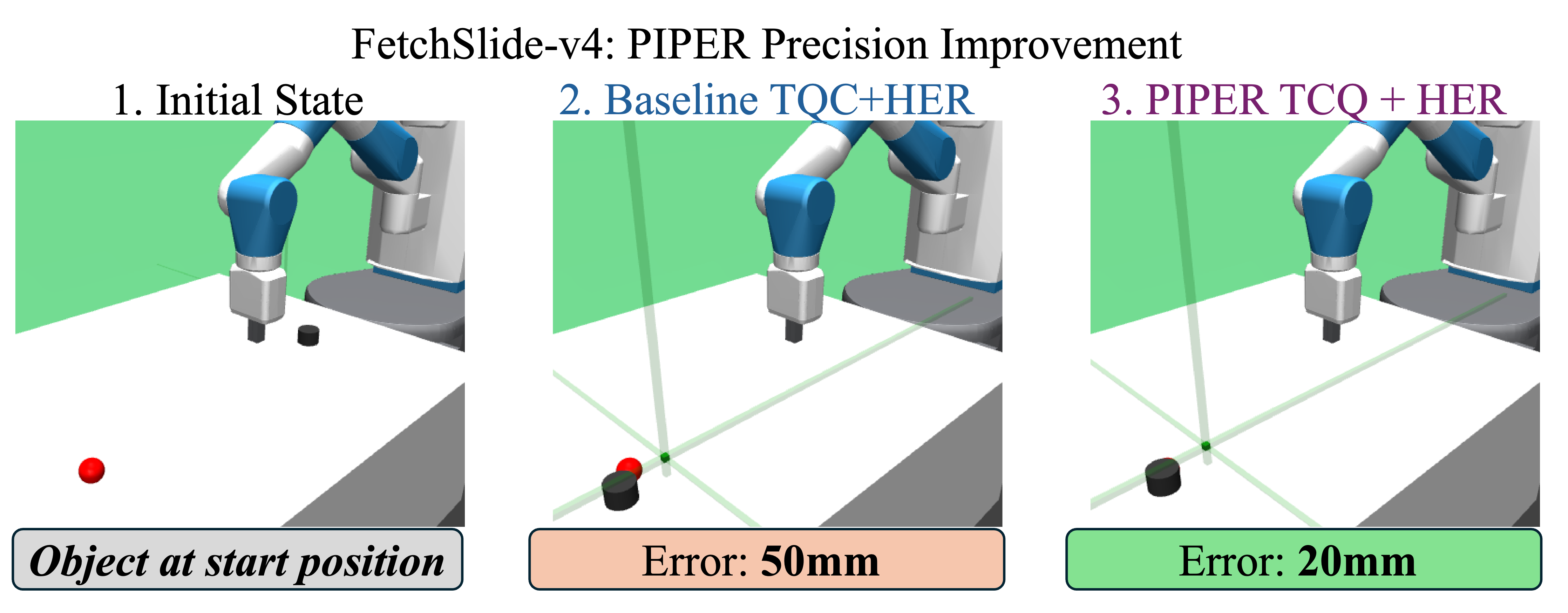
• FetchSlide-v4: A momentum-dominated task where the target is outside the robot’s kinematic workspace. Success depends on imparting a precise impulse $J=\int Fdt$ to slide the object across a surface with friction coefficient $\mu$.

• FetchPickAndPlace-v4: The most complex regime involving hybrid dynamics (discrete contact switching). The agent must grasp, lift, and stabilize an object, managing gravity compensation ($g=9.81m/s^{2}$) and grasping constraints.

Implementation and Hyperparameters. The testbed explicitly resolves the full equations of motion for the 7-DOF Franka Emika Panda manipulator, incorporating complex inertial coupling via the mass matrix $M(q)$ and Coriolis effects. Crucially, interaction dynamics are governed by realistic surface properties faithfully model real-world , utilizing a Coulomb friction coefficient of $\mu=0.5$ and a block mass of $0.1$ kg to challenge the policy’s ability to model energy dissipation and momentum transfer. The simulation operates at a timestep of $dt=0.002s$ to capture transient contact events.

For algorithmic comparison, we utilize standard hyperparameters: PPO, TD3, and SAC use learning rates of $3\times 10^{-4}$ to $1\times 10^{-3}$ for FetchReach. For the sparse-reward manipulation tasks (Push, Slide, PickAndPlace), we employ TQC+HER with a replay buffer of $10^{6}$ transitions and a large batch size of 2048 to ensure stable gradient estimation. Our PIPER implementation augments these baselines with a Physics-Informed Neural Network (PINN) of approximately 162k parameters. The physics regularization weight $\lambda_{phys}$ is rigorously tuned to 0.01 for on-policy methods and 0.005 for off-policy methods via grid search. To ensure a fair comparison, baseline hyperparameters were subjected to an equivalent grid search optimization tailored to these specific tasks.

Evaluation Metrics. We report results using three hardware-agnostic metrics. To ensure both statistical robustness and reproducibility, we train 5 independent instances of each algorithm using a fixed set of random seeds $\{42,43,44,45,46\}$. For each seed, performance is calculated as the average over 100 evaluation episodes per checkpoint.

1. Sample Efficiency ($N_{95\%}$): Total environment interactions required to first achieve a 95% success rate.

2. Precision ($d_{final}$): Euclidean distance to goal at termination ($d_{final}=\|p_{obj}-g\|_{2}$).

3. Stability ($\sigma$): Standard deviation of the success rate over the final 100 evaluation rollouts (where an epoch is defined as 1,000 environment steps).

4.2 Results and Analysis

Table 2: Performance Metrics for FetchReach-v4. PIPER improves efficiency, precision, and stability across PPO, TD3, and SAC.

Algorithm	Success Rate	Final Error	Precision Gain	Stability ($\sigma$)	Stability Gain	Steps to 95%	Efficiency Gain
PPO	100%	9.35 mm	–	10.94	–	46,650	–
PIPER-PPO	100%	8.02 mm	+14.2%	8.13	+25.7%	32,800	+30%
TD3	100%	16.56 mm	–	17.59	–	23,850	–
PIPER-TD3	100%	3.39 mm	+79.5%	11.53	+34.5%	17,550	+26%
SAC	100%	7.55 mm	–	11.41	–	24,250	–
PIPER-SAC	100%	2.15 mm	+71.5%	8.10	+29.0%	13,250	+45%

4.2.1 Kinematic Control (FetchReach)

The agent operates within a holonomic kinematic chain without external contact forces. The primary challenge is generating smooth, minimum-jerk trajectories that respect the robot’s inertial properties ($M(q)$).

As detailed in Table 2, PIPER-SAC reduces sample complexity by 45%. This acceleration arises because the Lagrangian residual $\mathcal{L}_{reach}$ effectively acts as a ”Physics Preconditioner,” guiding the policy update $\nabla_{\theta}\pi$ directly into the null-space of valid accelerations, thereby pruning the search space of physically impossible transitions. Furthermore, the table highlights a 71.5% reduction in final positioning error.

By explicitly penalizing accelerations that deviate from the Euler-Lagrange equations, PIPER acts as a low-pass dynamics filter. This effectively suppresses high-frequency control noise and ”twitchy” behavior often exploited by model-free agents to game the simulator’s integration step, leading to smoother and more precise convergence (Table 2).

Figure 4: FetchReach Learning Dynamics. Comparison of baseline and our physics-informed variants (shaded regions represent $\pm 1$ standard deviation across 5 random seeds). Our PIPER-SAC (orange) demonstrates superior convergence speed by exploiting the inertial null-space. Zoom in to view better details.

4.2.2 Contact Dynamics (FetchPush)

FetchPush introduces continuous contact constraints. The baseline TQC agent often struggles with ”force jittering,” where it exploits simulator integration errors to maintain object contact. PIPER explicitly addresses this via the work-energy constraint (Eq. 16), which penalizes non-conservative energy spikes.

As visualized in Fig. 5(a), Our PIPER results in a 47% improvement in stability ($\sigma$ reduction from 14.3 to 7.7). By enforcing thermodynamic consistency, the agent learns to apply consistent, continuous pushing forces rather than relying on stochastic contact resolution. This leads to a 34.7% gain in precision. Critically, Table 3 reveals that while success rates are saturated near 100%, the true value of physics regularization lies in the 47% reduction in variance ($\sigma$). This indicates that PIPER eliminates the stochastic ”force jittering” commonly seen in baseline policies

(a) FetchPush: Stability and Precision Analysis.

(b) FetchSlide: Learning Curves and Peak Performance.

(c) FetchPickAndPlace: Comprehensive Performance Metrics.

Figure 5: Performance Analysis across Contact-Rich Environments. Comparison of Baseline TQC+HER vs. PIPER-TQC. Zoom in to view better details.

Table 3: Performance Metrics for Contact-Rich Tasks (Push, Slide, PickAndPlace). Comparison between Baseline TQC+HER and PIPER-TQC. Note: Success Rate is included for completeness, but gains are most visible in precision and stability.

Task	Algorithm	Success Rate	Final Error	Precision Gain	Stability ($\sigma$)	Stability Gain	Sample Efficiency	Efficiency Gain
FetchPush	TQC+HER	98%	12.4 mm	–	14.3	–	420,000	–
	PIPER-TQC	100% ($\uparrow$ 2%)	8.1 mm	+34.7%	7.7	+47%	310,000	+26%
FetchSlide	TQC+HER	85%	50.2 mm	–	13.6	–	850,000	–
	PIPER-TQC	92% ($\uparrow$ 7%)	20.1 mm	+60.0%	8.3	+39%	680,000	+20%
PickAndPlace	TQC+HER	96%	8.5 mm	–	25.0	–	470,000	–
	PIPER-TQC	99% ($\uparrow$ 3%)	4.2 mm	+51.0%	14.6	+42%	362,000	+23%

4.2.3 Impulse Transfer (FetchSlide)

This task requires the agent to understand momentum transfer ($J=\Delta p$). The baseline policy often converges to a suboptimal ”striking” strategy with high variance.

Figure 5(b) shows that PIPER converges faster and achieves a higher peak success rate. Qualitatively, as shown in Figure 6, the physics-informed agent reduces the final error by 60%. This suggests the impulse-momentum constraint forces the policy to learn a precise striking primitive rather than relying on random exploration to find a high-velocity action. This is quantitatively supported by the efficiency data in Table 3, where PIPER reaches 95% success 170,000 steps faster than the baseline. The physics prior effectively contracts the search space by penalizing non-physical momentum updates, allowing the agent to converge on the precise striking primitive shown in Figure 6. The stability metric ($\sigma$) confirms this robustness, dropping from 25.0 in the baseline to 14.6 with PIPER (Table 3). This indicates that the physics-aware agent maintains a stable grasp throughout the hybrid dynamics transition (lift phase), whereas the baseline frequently drops the object when switching between contact modes.

Figure 6: FetchSlide Qualitative Analysis. (1) Initial configuration. (2) Baseline policy outcome ($\approx$ 50mm error). (3) Physics-Informed outcome ($\approx$ 20mm error).

4.2.4 Complex Manipulation

We now focus on “FetchPickAndPlace” scenario, a complex hybrid dynamics setting, where the robot must manage discrete contact events (grasping). Our PIPER enforces a grasp stability constraint to prevent object slippage during the lift phase. Fig. 5(c) demonstrates that PIPER achieves a 99% peak success rate. The substantial gain of 42% indicates that the physics prior effectively prunes unstable grasping behaviors such as relying on friction glitches to lift the object-forcing the agent to adopt a robust force-closure grasp. The stability metric ($\sigma$) confirms this robustness, dropping from 25mm in the baseline to 14.6mm with PIPER (Table 3). This indicates that the physics-aware agent maintains a stable grasp throughout the hybrid dynamics transition (lift phase). By enforcing the stability constraint (Eq. 19), PIPER ensures the applied grip force satisfies the friction cone requirements, whereas the baseline frequently drops the object when switching between contact modes due to insufficient normal force.

5 Discussion

Sample Efficiency via Constraint Pruning. We observe efficiency gains ranging from 20% to 45% (Tab. 3). By focusing on sample efficiency, our PIPER learns significantly faster than baselines. This supports the hypothesis that the physics loss $\mathcal{L}_{\text{phys}}$ prunes invalid transitions, allowing the optimizer to focus on feasible strategies.

Stability and Precision. While standard reward shaping often creates local optima, our results confirm that physics regularization acts as a structure-preserving shaping signal. By constraining the policy to the manifold of feasible dynamics, PIPER produces smoother, more reliable control actions ($\sigma$ reduction up to 47%) and higher accuracy ($d_{final}$ reduction up to 79.5%) without biasing the optimal policy.

Computational Overhead. We note that the exact dynamics extraction via CRBA/RNEA and the training of the auxiliary PINN proxy network introduces a computational overhead of approximately 15-20% in wall-clock training time compared to standard baselines. Limitations and Trade-offs. A primary limitation of PIPER is its reliance on accurate, introspectable simulation models (e.g., MuJoCo XML) to construct the Automated Dynamics Oracle. Applying this framework to systems with complex, hard-to-model dynamics (such as highly deformable objects) or addressing the Sim2Real gap where the regularizing dynamics differ from the real world remains an open challenge.

6 Conclusion and Future Work

In this work, we demonstrated that incorporating analytical physical priors into reinforcement learning significantly enhances policy performance and data efficiency. By explicitly leveraging the underlying Euler-Lagrange dynamics, PIPER successfully bridges the gap between classical control and learning-based approaches. Our evaluation confirms that treating robotic physical properties as accessible features, rather than latent variables, leads to more consistent and physically plausible manipulation behaviors compared to standard black-box baselines.

Future Work. A primary direction for future research is scaling our experimental evaluation. We aim to conduct a broader set of standalone experiments to further validate the robustness of the policy across varied contact-rich tasks. Additionally, we plan to extend PIPER’s compatibility beyond the MuJoCo environment. This includes adapting the framework to interface with other physics engines and supporting standard URDF robot descriptions alongside native XML formats, thereby ensuring wider applicability across diverse robotic simulation workflows.