All-sky Search for Continuous Gravitational Waves from Isolated Neutron Stars in the First Part of the Fourth LIGO-Virgo-KAGRA Observing Run

Abstract

We present results from an all-sky search for continuous gravitational waves, using three different methods applied to the first eight months of LIGO data from the fourth LIGO-Virgo-KAGRA Collaboration’s observing run. We aim at signals potentially emitted by rotating, non-axisymmetric isolated neutron star in the Milky Way. The analysis spans a frequency range from 20 Hz to 2000 Hz and accommodates frequency derivative magnitudes up to $10^{-8}$ Hz/s. No statistically significant periodic gravitational wave signals were detected. We establish 95% confidence-level (CL) frequentist upper limits on the dimensionless strain amplitudes. The most stringent population-averaged strain upper limits reach $9.7\times 10^{-26}$ near 290 Hz, matching the best previous constraints from 250 to $\sim$1700 Hz while extending coverage to a much broader spin-down range. At higher frequencies, the new limits improve upon previous results by factors of approximately $\sim$1.6. These constraints are applied to three astrophysical scenarios: 1) the distribution of galactic neutron stars as a function of spin frequency and ellipticity; 2) the contribution of millisecond pulsars to the “GeV excess” near the galactic center; and 3) the possible dark matter fraction composed of nearby inspiraling primordial binary black holes with asteroid-scale masses.

I Introduction

We report new results of all-sky searches for continuous-wave (CW), nearly monochromatic gravitational waves using the data from the two LIGO detectors [2] during the first eight months (O4a) of the fourth LIGO-Virgo-KAGRA observing run. Potential sources include conventional but slightly non-axisymmetric, fast-spinning galactic neutron stars [67, 86, 107] and more exotic sources: very nearby and light primordial binary black hole systems [95]. All-sky searches for continuous gravitational waves from isolated neutron stars have been carried out in Advanced LIGO and Virgo data previously [13, 15, 14, 16, 112, 129, 58, 59, 60, 143, 17, 19, 127, 135, 1, 92]. The all-sky results presented here are the most sensitive to date in strain amplitude for the full frequency and frequency derivative parameter space covered, although less sensitive than some previous O3 searches in some subsets of that parameter space. All-sky searches for isolated gravitational CW sources belong to a suite of searches for quasi-monochromatic gravitational wave emitters from the galaxy and beyond (recent reviews: [134, 118, 122, 145]).

Three different semi-coherent search programs (“pipelines”) are used here: 1) PowerFlux [10, 11, 7, 12, 13, 15] with loose-coherence follow-up [61, 62] (templated); 2) FrequencyHough [15, 16, 19, 36] (templated); and 3) SOAP [42, 41] (hidden Markov model; non-templated). Collectively, these searches span a signal frequency band from 20 Hz to as high as 2000 Hz and allow frequency time derivative magnitudes as high as $10^{-8}$ Hz/s. Finding no credible signals from any search, we set upper limits on signal strain amplitudes and present astrophysical population inferences.

This article is organized as follows: Section II describes the data set used, including steps taken to mitigate extremely loud and relatively frequent instrumental glitches seen in the O4 LIGO data, a phenomenon also seen in third observing run (O3). Section III describes the methodologies used by the PowerFlux, FrequencyHough and SOAP search pipelines, while Section IV describes the methodologies used to interpret the results for different astrophysical populations. Section V presents the results of the searches, and Section VI interprets those results astrophysically. Section VII concludes with a summary of the results and prospects for future searches. The appendices provide more details on the search methodologies and validations.

II Data sets used

We report here results from searches of early LIGO data from the fourth observing run O4 [48, 66, 82]. Intrinsic detector noise has been reduced with respect to O3 levels, especially at frequencies higher than $\sim$100 Hz for the LIGO Hanford (H1) and LIGO Livingston (L1) interferometers. The O4 run began on May 24, 2023 and completed on November 18, 2025. This article presents results based on analysis of the first eight months of O4, known as the O4a period, which ended on January 16, 2024, at the start of a 2-month commissioning break.

The Virgo interferometer [26] did not operate during the O4a period, while the KAGRA interferometer [28] observed for only one month and with a much lower sensitivity than the LIGO interferometers. Hence, results from analyzing only the H1 and L1 data are presented here. We use data from the GDS-CALIB_STRAIN_CLEAN frame channel, corresponding to the standard online calibration [138, 130, 131, 141] with some noise subtraction applied [139, 137, 5].

Prior to searching for CW signals, the quality of the O4a data was assessed [126] and steps taken to mitigate the effects of instrumental artifacts, including vetoes of data segments with severe instrumental disturbances [70]. As in previous Advanced LIGO observing runs [54], instrumental “lines” (sharp peaks in fine-resolution run-averaged H1 and L1 spectra) are marked, and where possible, their instrumental or environmental sources identified [69]. The resulting database of artifacts proved helpful in eliminating spurious signal candidates emerging from the search.

Another type of artifact observed in the O4a data for both H1 and L1 were relatively frequent and loud “glitches” (short, high-amplitude instrumental transients) with most of their spectral power lying below $\sim$500 Hz. As was true in the O3 run, these transients can be loud enough and frequent enough to distort the noise floor appreciably in spectra taken over even long durations. To mitigate the effects of these glitches on O4 CW searches at frequencies, a glitch-gating algorithm [55] was applied by the PowerFlux and SOAP pipelines that is similar in approach, but somewhat different in design, from the approach [128] used in an O3 Einstein@Home all-sky search [127]. The algorithm iteratively excises short intervals of time around detected glitches, verifying that the resulting change in spectral noise is an improvement, starting with the loudest glitches and considering smaller glitches in turn, until the preserved live time falls below 99%, or no further loud glitches are detected. The excision is carried out via inverse Planck windowing in which the data stream is tapered to zero over a half-second interval preceding the glitch and tapering back to unexcised data over another half second following the glitch. The tapered intervals are included when computing the deadtime losses capped at 1%. Glitches are defined by large excursions from nominal values of absolute power or of whitened power in the 25-50 Hz and 70-110 Hz bands. “Hardware injections” (see Section III.5) are recovered with higher signal-to-noise ratio (SNR) in gated data than in the original, ungated data, as was true for the O3 data [150]. The FrequencyHough method, on the other hand, uses pre-processed input data where short time-domain disturbances have been subtracted following the procedure described in [35], see Sec. III.3 for more details.

All three search methods described in Section III use “short” discrete Fourier transforms of the strain time series, but with different choices of coherence time. For the computationally demanding semi-coherent searches (PowerFlux and FrequencyHough), there is a tradeoff between sensitivity and cost that disfavors longer coherence times at higher frequencies. The PowerFlux method uses three distinct choices of coherence time: 7200 s for 20-475 Hz, 3600s for 475-1475 Hz and 1800s for 1475-2000 Hz when computing “short” Fourier transforms (SFTs); the 7200 s SFTs are created from gated data. The FrequencyHough method uses a band-sampled-data (BSD [117]) approach that enables many more discrete choices of SFT coherence time, ranging from 16384 s at 20 Hz to 2048 s at 1024 Hz, with discrete steps at each 1 Hz boundary. The SOAP method uses spectral averages over 1-day intervals based on 1800s SFTs created from gated data.

III Search Methodology

The three methods applied in this analysis have been used previously and described in detail elsewhere (see sections III.2-III.4 below for references). In the following subsections, we summarize briefly their different approaches after describing the signal model used explicitly in the PowerFlux and FrequencyHough semi-coherent searches. We also present validation of the search programs via recovery of “hardware injections.”

III.1 Signal model

The signal templates used in the PowerFlux and FrequencyHough searches assume a classical model of a spinning neutron star with a time-varying quadrupole moment that produces circularly polarized gravitational radiation along the rotation axis, linearly polarized radiation in the directions perpendicular to the rotation axis and elliptical polarization for the general case. The star’s orientation, which determines the polarization, is parametrized by the inclination angle $\iota$ of its spin axis relative to the detector line-of-sight and by the angle $\psi$ of the axis projection on the plane of the sky. The linear polarization case ($\iota=\pi/2$) is the most unfavorable because the gravitational wave flux impinging on the detectors is smallest for an intrinsic strain amplitude $h_{0}$, possessing eight times less incident strain power than for circularly polarized waves ($\iota=0,\>\pi$).

The strain signal model $h(t)$ for a periodic source is assumed to be the following function of time $t$:

$$h(t) = h_{0}\bigl(F_{+}(t,\alpha_{0},\delta_{0},\psi)\frac{1+\cos^{2}(\iota)}{2}\cos(\Phi(t))\vphantom{\frac{1+\cos^{2}(\iota)}{2}}$$ (1)

$$\quad\>+F_{\times}(t,\alpha_{0},\delta_{0},\psi)\cos(\iota)\sin(\Phi(t))\bigr)\textrm{\penalty 10000\ ,}$$

where $h_{0}$ is the intrinsic strain amplitude, $\Phi(t)$ is the signal phase, $F_{+}$ and $F_{\times}$ characterize the detector responses to signals with “$+$” and “$\times$” quadrupolar polarizations [10], and the sky location is described by right ascension $\alpha_{0}$ and declination $\delta_{0}$.

In a rotating triaxial ellipsoid model for a star at distance $r$ spinning at frequency $f_{\rm rot}$ about its (approximate) symmetry axis ($z$), the amplitude $h_{0}$ can be expressed as

$$h_{0} = {4\,\pi^{2}G\epsilon I_{\rm zz}f_{\rm GW}^{2}\over c^{4}r}$$ (2)

$$= [1.1\times 10^{-26}]\Bigl[{\epsilon\over 10^{-6}}\Bigr]\Bigl[{I_{\rm zz}\over I_{0}}\Bigr]\Bigl[{f_{\rm GW}\over{\rm 100\>Hz}}\Bigr]^{2}\Bigl[{1\>{\rm kpc}\over r}\Bigr],$$

where $I_{0}=10^{38}$ kg$\cdot$m² (10⁴⁵ g$\cdot$cm²) is a nominal neutron star moment of inertia $I_{\rm zz}$ about $z$, and the gravitational radiation is emitted at frequency $f_{\rm GW}=2\,f_{\rm rot}$. The equatorial ellipticity $\epsilon$ is a convenient, dimensionless measure of stellar non-axisymmetry:

$$\epsilon\quad\equiv\quad{I_{xx}-I_{yy}\over I_{zz}}.$$ (3)

The phase evolution of the signal is given in the reference frame of the Solar System barycenter (SSB) by the second-order approximation:

$$\Phi(t)=2\pi\left(f_{\textrm{GW}}\cdot(t-t_{0})+\dot{f}_{\rm GW}\cdot(t-t_{0})^{2}/2\right)+\phi\textrm{\penalty 10000\ ,}$$ (4)

where $f_{\textrm{GW}}$ is the SSB source frequency, $\dot{f}_{\rm GW}$ is the first frequency derivative (which, when negative, is termed the spin-down), $t$ is the SSB time, and the initial phase $\phi$ is computed relative to reference time $t_{0}$. When expressed as a function of the local time of ground-based detectors, Eq. 4 acquires sky-position-dependent Doppler shift terms.

All known isolated pulsars spin down more slowly than the maximum value of $|\dot{f}|_{\textrm{\mbox{\tiny{max}}}}$ used here, and as seen in the results section, the equatorial ellipticity required for higher $|\dot{f}|$ is improbably high for a source losing rotational energy primarily via gravitational radiation at low frequencies. More plausible is a source with spin-down dominated by electromagnetic radiation energy loss, but for which detectable gravitational radiation is also emitted.

III.2 The PowerFlux search

The PowerFlux search starts with a semi-coherent stage [10, 13, 15, 7] and uses loose coherence to follow up outliers [61, 62]. In brief (see Appendix A for details), strain power is summed over many SFTs after correcting for Doppler modulations, for a large bank of templates based on sky location, frequency, frequency derivative and stellar orientation. The maximum strain powers detected over the entire sky and for all frequency derivatives in each narrow frequency sub-band (see Table 7 in Appendix A for the frequency-dependent widths) define strict frequentist upper limits. The search is carried out over the frequency band 20-2000 Hz and the frequency derivative range $[-10^{-8}$–$10^{-9}]$ with three discrete choices of SFT coherence time (see Appendix A). Figure 1 depicts the parameter space coverage for the PowerFlux search and for the FrequencyHough search described in Sec. III.3.

Figure 1: Comparison of frequency and spin-down ranges for the templated searches presented here, along with those of previous Einstein@Home searches [127, 1, 92] of the O3 data discussed in section V.4. The dark-green-shaded rectangle with fine gridding bars shows the 20–2000 Hz and $-10^{-8}$–$10^{-9}$ Hz/s range for the O4a PowerFlux search. The slightly taller but narrower yellow rectangle shows the region searched in the O4a FrequencyHough analysis. The smaller rectangles with diagonal hatching show the three Einstein@Home search ranges for the O3 data [127, 1, 92], which have small variations in $\dot{f}_{\rm GW}$ ranges searched. The white curves show corresponding nominal ellipticities implied by a given frequency and spin-down for the gravitar model in which all rotational energy loss can be attributed to gravitational wave emission due to a mass quadrupole. Searching for high ellipticity values at a given frequency requires a high $\dot{f}_{\rm GW}$ range. (color online)

The PowerFlux pipeline has a hierarchical structure that permits systematic follow-up of loud outliers from the initial stage. The later stages improve intrinsic strain sensitivity by increasing effective coherence time while dramatically reducing the parameter space volume over which the follow-up is pursued. The pipeline uses loose coherence [61] with stages of improving refinement via steadily increasing effective coherence times. Any outliers that survive all stages of the search pipeline are examined manually for contamination from known instrumental artifacts and for evidence of contamination from a previously unknown single-interferometer artifact. Those for which no artifacts are found are subjected to further follow-up described below.

In the pipeline’s initial stage, the main PowerFlux algorithm [10, 13, 15, 11, 7, 12] establishes upper limits and produces lists of outliers. The program sets strict frequentist upper limits on detected strain power in circular and linear polarizations that apply everywhere on the sky except for small regions near the ecliptic poles, where signals with small Doppler modulations can be masked by stationary instrumental spectral lines. The procedure defining these excluded regions is described in [7] and applies to less than $0.2$% of the sky over the entire run, where the precise shapes of the regions near the poles depend on assumed signal frequency and spin-down. Initial outliers are defined by a joint H1-L1 signal-to-noise ratio (SNR) greater than a threshold of 7, with consistency among corresponding H1, L1 and joint H1-L1 outliers (criteria described in section III.2.2). These outliers are then followed up with a loose-coherence detection pipeline [61, 62, 7], which is used to reject or confirm the outliers.

III.2.1 Upper limits determination

The 95% confidence-level (CL) upper limits presented in section V.1 are reported in terms of the worst-case value of $h_{0}$ (linear polarization) and for the most sensitive case of circular polarization.

These upper limits, produced in stage 0, are based on the overall noise level and largest outlier in strain found for every template in each narrow sub-band in the first stage of the pipeline. Sub-bands are analyzed by separate instances of PowerFlux [7]

To allow robust analysis of the entire spectrum, including regions with severe spectral artifacts, a Universal statistic algorithm [63, 13] is used for establishing upper limits. The algorithm is derived from the Markov inequality and shares its independence from the underlying noise distribution. It produces upper limits less than $5$% above optimal in case of Gaussian noise. In non-Gaussian bands, it can report values larger than what would be obtained if the true underlying distribution were known, but the upper limits are always at least 95% valid. Appendix A.2 gives details on the validation of the PowerFlux upper limits derived in this analysis.

III.2.2 Outlier follow-up

A follow-up search for detection is carried out for high-SNR outliers found in stage 0. The outliers are subject to an initial coincidence test. For each outlier with $\textrm{SNR}>7$ in the combined H1 and L1 data, we require there to be outliers in the individual detector data of the same small sky patch, approximately square with side length $\sim$30 mrad $\times$ (100 Hz / frequency) that have $\textrm{SNR}>5$ and match the parameters of the combined-detector outlier within 2.5 mHz in frequency and $3\times 10^{-10}$ Hz/s in spin-down. The combined-detector SNR is additionally required to be above both single-detector SNRs, in order to suppress single-detector instrumental artifacts, except for unusually loud outliers (H1, L1 and combined SNRs all greater than 20).

The identified outliers using combined data are then passed to the follow-up stage using a loose-coherence algorithm [61] with progressively improved determination of frequency, spin-down, and sky location.

As the initial stage 0 sums only powers, it does not use the relative phase between interferometers, which results in some degeneracy among sky position, frequency, and spin-down. The first loose-coherence follow-up stage (1) demands greater temporal coherence within each interferometer, which should boost the SNR of viable outliers, but combines H1 and L1 power sums incoherently, The subsequent stage (2) uses combined H1 and L1 data coherently, providing tighter bounds on outlier location. Details concerning parameters used in outlier follow-up may be found in Table 8 in Appendix A.1. Validation of the PowerFlux loose-coherence outlier follow-up is described in Appendix A.3.

As in previous PowerFlux analyses with loose-coherence follow-up [13, 15], only a mild influence from parameter mismatch is expected, as the parameters are chosen to accommodate the worst few percent of injections. The follow-up procedure establishes wide margins for outlier follow-up. For example, when transitioning from the semi-coherent stage 0 to the loose-coherence stage 1 below 475 Hz, the effective coherence length increases by a factor of 4. The average true signal SNR should then increase by more than $40$%. But the threshold used in follow-up is only 15–20%, depending on frequency, which accommodates unfavorable noise conditions, template mismatch, and detector artifacts.

As in the O3a PowerFlux search, we apply a combination of manual inspection and systematic deep follow-up to any outliers that survive the second stage of follow-up. After a simple clustering in the parameter space of ($f$, $\dot{f}$, $\alpha$, $\delta$), the loudest outlier in each cluster is examined manually via a “strain histogram” [135] and frequency trajectory graph that helps assess the degree of contamination in the putative outlier signal by known or obvious instrumental contamination. Surviving outliers not exhibiting clear contamination are subjected to a final follow-up method using the Python-based PyFstat [84, 33] software infrastructure to combine a MCMC approach [34, 133] with semi-coherent summing of the well known $\mathcal{F}$-statistic detection statistic [81]. In this approach, the parameter space near to those values from a stage-2 survivor is sampled randomly according to a certain probability density function determined by the $\mathcal{F}$-statistic likelihood function. We follow the same implementation [133] applied to the O3a PowerFlux outliers [17].

Briefly, the O4a observation time is divided into $N_{\textrm{seg}}$ segments, for each of which the $\mathcal{F}$-statistic is computed over a coherence time approximately equal to the observation time divided by $N_{\textrm{seg}}$. For each point sampled in parameter space, the sum of the $\mathcal{F}$-statistic values is computed to form a total detection statistic. This procedure is repeated, decreasing the number of segments (increasing the coherence time), using the resulting MCMC-maximized $\mathcal{F}$-statistic sum as the seed for the next stage, with a consequent reduction in parameter space volume searched. For this O4a analysis we choose six successive stages of follow-up with decreasing values of $N_{\textrm{seg}}$ = 500 (coherence time of 0.47 day), 250, 150, 60, 5 and 1. A random sample of 600 off-source sky locations having the same declination as the putative signal direction, but separated by more than 90 deg from that direction, is used to determine a non-signal expectation for the background distributions in the same frequency band [133]. A Bayes factor $B_{\rm SN}$ is computed from the change in $\mathcal{F}$-statistic values for a nominal signal compared to the empirical background distribution in the last stage ($N_{\textrm{seg}}$=5 to $N_{\textrm{seg}}$=1).

III.3 The FrequencyHough search

The FrequencyHough pipeline is a semi-coherent procedure in which interesting outliers are selected in the signal parameter space, and then are followed-up in order to confirm or reject them. This method has been used in several past all-sky searches of Virgo and LIGO data [3, 15, 16, 112, 19]. A detailed description of the methodology can be found in [36], but some changes have been made to the procedure, in order to improve the sensitivity of the search and also to optimize its computational cost. We thus describe in the following the main analysis steps, leaving the details to Appendix B.1. A relevant novelty with respect to the past is that the FrequencyHough pipeline now uses the BSD framework [117]. This change allows us to evaluate Fast Fourier Transforms (FFTs) with duration $T_{\mathrm{FFT}}$ optimized for each 1 Hz band (the previous implementation used four different bands, each of fixed $T_{\mathrm{FFT}}$ duration). This duration fixes the coherent time of the search, hence a non optimal choice of this parameter would reduce the final sensitivity.

From the collection of FFTs computed over the run duration, the so-called “peakmap” is built. For each sky position the time-frequency peaks of the peakmap are properly shifted, to compensate for the Doppler effect due to the detector motion [36]. The shifted peaks are then fed to the FrequencyHough algorithm [36], which transforms each peak to the frequency/spin-down plane of the source. A new implementation of the FrequencyHough algorithm has been used for the first time in this search, see Appendix B.2 for more details. The output of a FrequencyHough   transform is a 2-D histogram in the frequency/spin-down plane of the source. Outliers, that are statistically significant points in this plane, are selected using a criterion described in Appendix B.1. As in past analyses [15, 16], coincidences among outliers of the two detectors are required, using a distance metric $d_{\rm FH}$ built in the four-dimensional parameter space of sky position $(\lambda,\penalty 10000\ \beta)$ (in ecliptic coordinates), frequency $f$ and spin-down $\dot{f}$. Coincident outliers are ranked according to the value of a specific statistic and the most significant are selected and subject to the follow-up.

III.3.1 Follow-up

The FrequencyHough follow-up runs on each outlier of each coincident pair. It is based on the construction of a new peakmap, over $\pm 3$ coarse bins around the frequency of the outlier, with a tripled $T_{\rm FFT}$ with respect to the all-sky stage. This new peakmap is built after heterodyning the data for the Doppler and spin-down (or spin-up) of the outlier. A refined sky grid is then constructed around the outlier position, spanning $\pm 3$ coarse bins, to account for uncertainties in the outlier’s parameters. For each point on this refined grid, we correct the peakmap by shifting the frequency peaks to remove the residual Doppler. Each corrected peakmap is the input for the FrequencyHough transform, which explores the relevant ranges in frequency and spin-down ($\pm±3$ coarse bins in both dimensions). Among all the resulting FrequencyHough histograms, the most significant peak associated with a refined set of parameters is selected and passed on for further post-processing steps to reduce the number of false outliers as described in [19] and in Appendix B.3. Only those outliers that pass all these tests proceed to the subsequent follow-up stages, where the coherence time is further increased. These additional stages are carried out with PyFstat [34, 84, 102] in a similar way to what is described in Sec. III.2.

III.3.2 Upper limits

“Population averaged” upper limits are computed for every 1 Hz sub-band in the range of the search (i.e., 10–1024 Hz). First, for each detector we use the following analytical relation (where an error in the numerical coefficient has been corrected w.r.t. the original formula presented in [36], see Appendix B.5):

$$h_{\mathrm{UL},95\%}\approx\frac{4.71}{N^{1/4}}\sqrt{\frac{S_{n}(f)}{T_{\rm FFT}}}\sqrt{\rm CR_{\rm max}+1.6449},$$ (5)

where $N=\mathrm{round}\left(\frac{T_{\mathrm{obs}}}{T_{\mathrm{FFT}}}\right)$, $S_{n}(f)$ is the detector average noise power spectrum, computed through a weighted mean over time segments of duration $T_{\rm FFT}$ (in order to take into account noise non-stationarity), and $\rm CR_{\rm max}$ is the maximum outlier Critical Ratio (CR) for each 1 Hz band. The coefficient 4.71 has been obtained taking the parameter $\theta_{\mathrm{thr}}=2.5$ (the values of $p_{0},\penalty 10000\ p_{1}$ directly depend on it), while the term 1.6449 comes from taking the confidence level parameter $\Gamma=0.95$. For each 1 Hz band, the final upper limit is the worse among those computed separately for Hanford and Livingston. Such upper limits implicitly assume an average over the source population parameters.

As verified through a detailed comparison based on LIGO and Virgo O2 and O3 data, this procedure produces conservative upper limits with respect to those obtained through the injection of simulated signals, which is computationally more intensive [111]. This conservativeness has been verified also through software injections for the first part of the fourth observing run for a set of 40 1 Hz frequency bands, showing that the upper limits estimation given by Eq. eq:hul overestimates limits obtained by performing software injections across the whole search frequency band, see Appendix B.7 for more details.

III.4 The SOAP search

SOAP [42] is a fast, model-agnostic search for long duration signals based on the Viterbi algorithm [140]. It is intended as both a rapid initial search for isolated NSs, quickly providing candidates for other search methods to investigate further, as well as a method to identify long duration signals which may not follow a conventional model of CW frequency evolution. In its simplest form SOAP analyzes a spectrogram to find the continuous time-frequency track which gives the highest sum of fast Fourier transform power. If there is a detectable signal present within the data, then this track is the most likely to correspond to that signal. The search pipeline consists of three main stages, the initial SOAP search [42], the post processing step using convolutional neural networks [40] and a parameter estimation stage [41].

III.4.1 Data preparation

The calibrated detector data are used to create a set of H1 and L1 SFTs with a coherence time of 1800 s. The power spectra of these SFTs are then summed over one day, i.e., over up to 48 SFTs. Assuming that the signal remains within a single bin over the day, this averages out the antenna pattern modulation and increases the SNR in a given frequency bin. As the frequency of a CW signal increases, the magnitude of the daily Doppler modulation also increases, therefore the assumption that a signal remains in a single frequency bin within one day no longer holds. Hence, the analysis is split into 4 separate bands (40-500 Hz, 500-1000 Hz, 1000-1500 Hz, 1500-2000 Hz) where for each band the Doppler modulations are accounted for by taking the sum of the powers in adjacent frequency bins. For the bands starting at 40, 500, 1000 and 1500 Hz, the sum is taken over every one (no change), two, three and four adjacent bins respectively such that the resulting time-frequency plane has one, two, three or four times the original bin width. The broad bands are further split into ‘sub-bands’ of widths 0.1, 0.2, 0.3 and 0.4 Hz wide respective to the four band sizes above. These choices ensure that the maximum yearly Doppler shift $\Delta f_{\rm{orb}}^{(\rm{max})}$ is half the sub-band width, where the maximum is given by

$$\Delta f_{\rm{orb}}^{(\rm{max})}=f\frac{v_{\rm{orb}}^{\rm{(max)}}}{c}\lesssim 10^{-4}f,$$ (6)

where $v_{\rm{orb}}^{\rm{(max)}}$ is the maximum orbital velocity of the earth relative to the source, $c$ is the speed of light and $f$ is the initial pulsar frequency. The sub-bands overlap by half of the sub-band width such that any signal should be fully contained within a sub-band.

III.4.2 Search pipeline

SOAP searches through each of the summed and narrow-banded spectrograms described in Sec. III.4.1, returning four main outputs for each sub-band: the Viterbi track, the Viterbi statistic, the Viterbi map and a convolutional neural network (CNN) statistic. The Viterbi statistic from the core pipeline and the CNN statistc from the CNN followup are used to select candidates for further analysis, as described in Sec. III.4.3. For more details on the search algorithm see Sec. C.

III.4.3 Candidate selection

At this stage there is a set of Viterbi statistics and CNN statistics for each sub-band that is analysed, from which a set of candidate signals is selected for followup. Before doing this, any sub-bands that contain known instrumental artifacts are removed from the analysis. The sub-bands corresponding to the top 1% of the Viterbi statistics from each of the four analysis bands are then combined with the sub-bands corresponding to the top 1% of CNN statistics, leaving us with a maximum of 2% of the sub-bands as candidates. It is at this point where we begin to reject candidates by manually removing sub-bands that contain clear instrumental artifacts and cross the detection threshold for either the Viterbi or CNN statistic. There are a number of features we use to reject candidates including: strong detector artifacts that only appear in a single detector’s spectrogram, broad ($>1/5$ sub-band width) long duration signals, individual time-frequency bins that contribute large amounts to the final statistic and very high-power signals in both detectors. Any remaining candidates are then passed on for parameter estimation.

III.5 Hardware injections

During the O4 run 18 hardware injections [44, 132, 39] were used to simulate particular CW signals, as part of detector response validation [39], including long-term phase fidelity. The injections were imposed via radiation pressure from auxiliary lasers [44]. For reference, Table 1 lists the key source parameters, including injected strain amplitude $h_{0}$, for the 14 injections relevant to this analysis (labeled Inj0-Inj12 and Inj14), namely those that simulate isolated neutron stars with nominal frequencies between 20 and 2000 Hz.

The last three columns of Table 1 state whether or not each injection in one of the three pipelines was detected, including survival of outlier follow-up. Entries marked with “-” indicate injection parameters outside the nominal search range for that pipeline. In addition, for the PowerFlux pipeline, which can set valid upper limits even in the presence of a loud signal, there is a column labeled “UL sig bin” giving an injection’s obtained PowerFlux 95% upper limit in the signal’s frequency bin. Ideally, the “UL sig bin” value should exceed the true injected amplitude $h_{0}$ for at least 95% of the injections. In this case, that statement holds for all 14 injections. The column labeled “UL ctrl bins” shows the average 95% ULs for the six nearest neighboring frequency subbands as a rough guide to the expected value in the absence of an injection (or true signal).

Inj	Frequency	Spindown	$\textrm{RA}_{\textrm{J}2000}$	$\textrm{DEC}_{\textrm{J}2000}$	$h_{0}$	P.F. UL	P.F. UL	Detected?
	Hz	nHz/s	degrees	degrees	true	sig bin	ctrl bins	P.F.	F.H.	SOAP
0	$265.574500$	$-4.15\times 10^{-3}$	$71.55193$	$-56.21749$	$4.01\times 10^{-26}$	$1.2\times 10^{-25}$	$1.3\times 10^{-25}$	N	N	N
1	$848.894997$	$-3.00\times 10^{-1}$	$37.39385$	$-29.45246$	$2.79\times 10^{-25}$	$3.0\times 10^{-25}$	$1.9\times 10^{-25}$	Y	Y	N
2	$575.163487$	$-1.37\times 10^{-4}$	$215.25617$	$3.44399$	$3.20\times 10^{-26}$	$1.6\times 10^{-25}$	$1.6\times 10^{-25}$	N	N	N
3	$108.857159$	$-1.46\times 10^{-8}$	$178.37257$	$-33.43660$	$1.30\times 10^{-25}$	$1.7\times 10^{-25}$	$1.5\times 10^{-25}$	Y	Y	N
4	$1387.220675$	$-2.54\times 10^{+1}$	$279.98768$	$-12.46662$	$4.90\times 10^{-25}$	$2.7\times 10^{-25}$	$2.8\times 10^{-25}$	Y	-	-
5	$52.808324$	$-4.03\times 10^{-9}$	$302.62664$	$-83.83914$	$3.99\times 10^{-25}$	$5.6\times 10^{-25}$	$2.7\times 10^{-25}$	Y	Y	Y
6	$144.494850$	$-6.73\times 10^{0\mathrm{\;\;\;}}$	$358.75095$	$-65.42262$	$3.20\times 10^{-25}$	$3.3\times 10^{-25}$	$1.5\times 10^{-25}$	Y	N	Y
7	$1220.276598$	$-1.12\times 10^{0\mathrm{\;\;\;}}$	$223.42562$	$-20.45063$	$7.16\times 10^{-26}$	$2.5\times 10^{-25}$	$2.5\times 10^{-25}$	N	-	N
8	$188.879028$	$-8.65\times 10^{0\mathrm{\;\;\;}}$	$351.38958$	$-33.41852$	$8.28\times 10^{-26}$	$1.3\times 10^{-25}$	$1.3\times 10^{-25}$	N	N	N
9	$763.847316$	$-1.45\times 10^{-8}$	$198.88558$	$75.68959$	$6.87\times 10^{-26}$	$1.8\times 10^{-25}$	$1.8\times 10^{-25}$	N	N	N
10	$26.320768$	$-8.50\times 10^{-2}$	$221.55565$	$42.87730$	$6.26\times 10^{-25}$	$1.6\times 10^{-24}$	$1.1\times 10^{-24}$	Y	Y	Y
11	$31.424632$	$-5.07\times 10^{-4}$	$285.09733$	$-58.27209$	$3.17\times 10^{-25}$	$5.0\times 10^{-25}$	$5.8\times 10^{-25}$	Y	N	N
12	$36.922850$	$-6.25\times 10^{0\mathrm{\;\;\;}}$	$331.85267$	$-16.97288$	$2.63\times 10^{-25}$	$3.7\times 10^{-25}$	$3.6\times 10^{-25}$	N	N	N
14	$1991.092151$	$-1.00\times 10^{-3}$	$300.80284$	$-14.32394$	$7.61\times 10^{-25}$	$8.6\times 10^{-25}$	$6.1\times 10^{-25}$	Y	-	N

Table 1: Key parameters of the hardware-injected simulated isolated-source continuous wave signals during the O4 data run (20-2000 Hz). The frequencies listed here correspond to the start of the run (GPS $1238166018$), but upper limits obtained by the search pipelines are indexed to frequency bands with a reference time at the approximate midpoint of the O4a epoch ($\sim$4 months later). Also shown are PowerFlux strain amplitude upper limits in the nominal signal bins and averaged over the six nearest control bins. The last three columns state whether or not an injection is detected by the three pipelines, including outlier follow-up. The relatively loud injection 6 at $\sim$144.5 Hz is detected by FrequencyHough as an initial-stage outlier, but is correctly vetoed in follow-up because of the overlap of the frequency band it covers with identified instrumental lines. The injection 11 is missed by FrequencyHough because the outliers it produces do not meet the strict distance criterion used to flag an injected signal as detected, see Appendix B.7.

IV Astrophysical interpretation – Methodology

Results of all-sky CW searches can be used to constrain certain astrophysical scenarios. In the following subsections, we discuss how constraints can be applied to models of 1) the population of galactic neutron stars; 2) the millisecond pulsar explanation for the GeV excess; and 3) the potential contributions to dark matter from asteroid-scale primordial black holes.

IV.1 Implications for the neutron star population

To interpret the astrophysical significance of strain amplitude upper limits, we translate them into constraints on the Galactic abundance of rapidly spinning, highly deformed neutron stars. For a neutron star with ellipticity $\epsilon$, emitting at GW frequency $f_{\rm GW}$, the horizon distance $r_{H}(\epsilon,f_{\rm GW})$ of the search is computed using Eq. 2:

$$r_{H}(\epsilon,f_{\rm GW})=\frac{4\pi^{2}GI_{zz}}{c^{4}}\frac{f_{\rm GW}^{2}\epsilon}{h_{\mathrm{UL}}^{95\%}(f_{\rm GW})},$$ (7)

Any neutron star emitting at frequency $f_{\rm GW}$ with ellipticity $\geq\,\epsilon$ located within the horizon distance $r_{H}(\epsilon,f_{\rm GW})$ is a detectable source. Assuming a spatial distribution of neutron stars allows us to find the mean fraction of the total Galactic population with ellipticity $\geq\,\epsilon$ that lie within the horizon distance $r_{H}$ (i.e., they are detectable) at frequency $f_{\rm GW}$, considering a nominal moment of inertia of $I_{zz}=I_{0}$. We denote this fraction by $\alpha(\epsilon,f_{\rm GW})$, defined as:

$$\alpha(\epsilon,f_{\rm GW})=\int_{0}^{r_{H}}\int_{0}^{\pi}\int_{0}^{2\pi}p_{\rm spatial}(r,\theta,\phi)\,r^{2}\,\sin\theta\,dr\,d\theta\,d\phi,$$ (8)

where $p_{\rm spatial}(r,\theta,\phi)$ represents the spatial distribution in spherical-polar coordinates centered at Earth. We consider four such distributions: the progenitor model in [108], which assumes a distribution for young neutron stars that follow the same spatial distribution as their progenitor stars and three specific models in [121], where the neutron star population is time-evolved in the galactic potential, accounting for natal kick velocities. The likelihood of a total of $N$ galactic neutron stars with ellipticity $\geq\,\epsilon$ and frequency $f_{\rm GW}$, given $n$ detections within the distance reach can be approximated as the following Poisson distribution: p( n — N, α(ϵ, f_GW) ) = (αN)ne- αNn!

As no detections are reported, we assert $n=0$ and use the Bayes’ theorem to construct the posterior distribution of $N$ as:

$$p(N|n=0,\alpha)\propto\exp(-\alpha N)p(N)$$ (9)

where the prior $p(N)$ is considered to be uniform. By construction, the posterior on $N$ is agnostic to any assumed spin or ellipticity distribution of the Galactic neutron star population. Instead, it provides constraints in the ($f_{\rm GW}$, $\epsilon$) space denoting the maximum number of sources exceeding ellipticity $\epsilon$ at emission frequency $f_{\rm GW}$. This prescription follows from [119].

IV.2 Implications for the GeV excess

In a similar vein, using the lack of detection of CW signals in this search, we can place constraints on the millisecond pulsar (MSP) hypothesis for the “GeV excess” of gamma radiation detected from near the Galactic Center. The enigmatic excess was first observed over a decade ago by the Fermi-LAT satellite [25, 27], which has led to two hypotheses being put forward to explain its origins: (1) annihilating Weakly Interacting Massive Particle (WIMP) dark matter [71, 76, 77, 72, 56, 45, 8] and (2) an unresolvable, electromagnetically faint population of MSPs [9, 46, 149, 115, 148]. If there is a concentration of electromagnetically dim MSPs in the Galactic Center that are invisible to Fermi-LAT, these pulsars could, in principle, still be detected via their gravitational-wave emission [47, 98]. While two recent works consider a stochastic gravitational-wave background arising from the Galactic Center [47, 38], we consider a more powerful way of constraining the GeV excess in this paper through individually resolvable MSPs [98]. We note that Ref. [87] recently reached a pessimistic conclusion regarding the possibility of seeing MSPs from the galactic center with current-generation detectors; however, we note that this is heavily dependent on the unknown MSP ellipticity distribution function.

To determine whether our searches could be sensitive to the GeV excess, we first calculate the probability of detecting gravitational waves from MSPs, $P_{\rm GW}$ by assuming frequency and ellipticity distributions $P(\log f_{\rm GW}),P(\log\epsilon)$ for the unknown MSP population:

$$P_{\rm GW} = \int_{\log f_{\rm min}}^{\log f_{\rm max}}d(\log f_{\rm GW})P(\log f_{\rm GW})$$ (10)

$$\times\int_{\log\epsilon_{\rm UL}(f)}^{\log\epsilon_{\rm max}}d(\log\epsilon)P(\log\epsilon)$$

where $f_{\rm min}$ and $f_{\rm max}$ refer to the minimum and maximum frequencies searched (we define a MSP to have a rotational frequency of at least 60 Hz [91]), $\epsilon_{\rm UL}(f)$ is the minimum detectable equatorial deformation in the CW searches at the center of the galaxy (8 kpc), and $\epsilon_{\rm max}$ is the maximum ellipticity to which a search is sensitive (fixed by max($\dot{f}_{\rm GW}$)). In this analysis, we assume a rotational frequency distribution for the unknown MSP that follows that of the known pulsars in the ATNF catalog [90], although there is significant selection bias towards higher frequencies of detected pulsars [89, 88]. In practice, however, the frequency distribution turns out to be an $\mathcal{O}(1)$ factor that is minor with respect to the ellipticity. We also assume a log10 exponential distribution $P(\log\epsilon)\propto\exp(-\Lambda\log\epsilon)$ for the ellipticities between $10^{-9}$ – motivated by the potentially minimum allowable ellipticity of a pulsar [147] – and $10^{-5}$ – motivated by the canonical maximum strain that a neutron star could support [103], with a power-law of $\Lambda=2.1$. The choice of $\Lambda$ is arbitrary, which reflects our ignorance of the ellipticity distribution of millisecond pulsars, but we study its impact on the constraints later in this section. For $\Lambda=2.1$, we simulate 100 distributions of ellipticities and take the average of the predicted $P_{\rm GW}$, which results in $P_{\rm GW}=5.88\times 10^{-5}$. The averaging allows us to take different realizations of the ellipticity distributions, ensuring robustness against random variations in the distributions.

The other ingredient necessary to put a constraint on the MSP hypothesis for the GeV excess is an estimation of the number of MSPs in the Galactic Center, which is called the gamma ray “luminosity function”. In this work, we use a standard prescription for the luminosity function [78]:

dNdL

∝P(L)= log10eσL2πLexp(-log102(L/L0) 2σL2), where $L$ is the luminosity, and $L_{0}$ and $\sigma_{L}$ are two free parameters. The choice of $L_{0}$ and $\sigma_{L}$ fixes the number of MSPs in the Galactic Center $N_{\rm MSP}$ [64]:

L_GCE = N_MSP∫_L_min^∞L P(L) dL. where $L_{\text{GCE}}\approx 10^{37}$ erg/s (see [98] for more details) and $L_{\rm min}$ is the minimum detectable luminosity by Fermi-LAT. Our work assumes that MSPs are emitting both gravitationally and electromagnetically.

In the absence of a detection, if $N_{\rm MSP}P_{\rm GW}>1$, we would have been able to detect a gravitational-wave signal from a millisecond pulsar (MSP) in the Galactic Center, and can thus rule out that choice of $L_{0}$ and $\sigma_{L}$.

IV.3 Implications for light primordial black holes

The CW searches presented here could also be sensitive to GWs emitted by quasi-infinite inspirals of asteroid-mass ultra-compact objects that could be primordial black holes [75, 51, 43, 53, 125, 50]. CW searches offer a promising avenue to probe the currently-unconstrained asteroid-mass regime for primordial black holes [94, 100, 101]. In particular, the FrequencyHough and PowerFlux methods require that the gravitational-wave signal follows a linear frequency evolution in order to detect it. Thus, binary systems with chirp masses $\mathcal{M}\lesssim\mathcal{O}(10^{-5})M_{\odot}$ would emit CW signals that would mimic those that arise from spinning up, non-axisymmetric rotating neutron stars [93, 30, 31, 29]. The upper limits derived in Fig. 2 can therefore be mapped to a constraint on the maximum distance away that we could have detected an inspiraling binary via the relation:

h_0=4d(G Mc2)^5/3(πfgwc)^2/3
≃1.61×10^-26​ [d10 pc]^-1​ [M10-6M⊙]^5/3​ [fgw50 Hz]^2/3, We can then compute a rate density $\mathcal{R}$ associated with the distance reach $d$, as described in [93], as a function of chirp mass. This rate density is independent of the existence and formation mechanisms of primordial black holes, and can be interpreted as a formation rate density, as opposed to a merger rate density that is frequently constrained in other gravitational-wave searches [4].

After obtaining a rate density, we must make the assumption that these rates would arise from the formation of primordial black holes. It is important to note that such constraints on primordial black holes is highly model-dependent. Using the rate density prescriptions for early two-body binaries, the dominant channel of primordial black hole formation relevant for this work, we can write [52, 53, 120, 79]:

$$\mathcal{R} = 5.28\times 10^{-7}\,\mathrm{kpc}^{-3}\mathrm{yr}^{-1}$$ (11)

$$\times\left(\frac{m_{1}}{M_{\odot}}\right)^{-32/37}\left(\frac{m_{2}}{m_{1}}\right)^{-34/37}\tilde{f}^{53/37}\penalty 10000\ ,$$

where $m_{2}<m_{1}$

$$\tilde{f}(m_{1},m_{2})\equiv f_{\text{PBH}}\left[f_{\text{sup}}f(m_{1})f(m_{2})\right]^{37/53}$$ (12)

is a parameter that relates to the fraction $f_{\text{PBH}}$ of dark matter that primordial black holes could compose and the mass distribution functions $f(m)$ for $m_{1}$ and $m_{2}$. $f_{\rm sup}$ is the suppression factor that accounts for various mechanisms affecting the binary orbital evolution throughout cosmic time [120], which could change their merger time or destroy them. For no suppression, $f_{\rm sup}=1$. We note that $f(m_{1})$, $f(m_{2})$ and $f_{\rm sup}$ depend on the specific primordial black hole formation model chosen; thus we decide to simply constrain $\tilde{f}$, which parameterizes our ignorance of these parameters, but allows interested readers to set constraints on $f_{\text{PBH}}$ for their chosen model.

V Search results

None of the three searches detected a credible CW signal. In the following subsections, we provide more details on these negative results.

V.1 The PowerFlux results

Carrying out the PowerFlux stage-0 analysis described above leads to a set of all-sky upper limits (95% CL) on strain amplitude for worst-case (unfavorable stellar spin orientation), linear polarization and for best-case, circular polarization. That analysis also leads to an initial set of outliers for follow-up with later analysis stages. Whether or not a particular narrow frequency band contains an outlier, the upper limits obtained remain valid. As shown in Table 1, hardware injections were reliably recovered when their injected strain was at least 0.6 times the recorded upper limit. Figure 13 in Appendix A presents strict PowerFlux upper limits on signals that are circularly polarized or linearly polarized, along with PowerFlux upper limits from searches in the O3 data set [17, 135]. The circular polarization limits are then used to estimate population-averaged upper limits, as described in Appendix A.

Outliers seen in the stage-0 search are followed up with loose-coherence stages of increasing effective coherence time, as described in section III.2.2, with the SNR expected to increase for true signals. Table 2 shows the counts of outliers seen at each stage for major sub-bands. In the presence of Gaussian noise and no signal, one expects the outlier counts to decrease monotonically with increasing stage as SNR increases are required for each advancement. For particular sub-bands, however, one can see count increases from at least two contributions, both associated with the finer sampling of parameter space in successive stages. 1) Hardware injections (section III.5) from a simulated signal naturally satisfy the SNR increase requirements demanded of a signal; and 2) stationary line artifacts of finite bandwidth can be compatible with signal templates having limited Doppler modulation or having partial cancellation between seasonal modulation and assumed frequency derivative for a certain region of the sky [10].

In the extreme, the number of outliers produced by a particular instrumental artifact can be so large as to make systematic follow-up impracticable and pointless. Artifacts include loud mechanical resonances, such as higher harmonics of violin modes, and especially loud hardware injections. The widest bands excluded lie in the regions of test-mass violin modes and their higher harmonics. Details concerning these vetoed bands can be found in Appendix A.4.

	20-60 Hz	60-475 Hz	475-1475 Hz	1475-2000 Hz
Stage 0	4916	7320	33407	16918
Stage 1	4267	13095	32466	6853
Stage 2	5816	2994	3350	3999
Outlier clusters	666	169	3252	191
HW injections	452	20	2513	29
Visible artifacts	145	142	706	149
PyFstat follow-up	69	7	33	13
PyFstat survivors	0	0	0	0

Table 2: Counts of PowerFlux outliers surviving different stages of the hierarchical follow-up for four frequency bands. Survivors from stage-2 follow-up are broken down into the categories of hardware injections, visible artifacts identified via strain histograms and candidates for PyFstat follow-up. Additional follow-up of these weak candidates, which appear in a visibly disturbed band of L1 data, was carried out using the MCMC PyFstat follow-up procedure described in section III.2.2. The PyFstat follow-up confirmed these 122 outliers to be uninteresting.

Nearly all outliers that survived all stages of the loose-coherence follow-up correspond to hardware injections (see Table 1) or lie in highly disturbed bands, for which contamination of the putative signal by an instrumental spectral line is apparent. To identify these contaminations, we construct “strain histograms” [17] in which the summed power over the observation period from a simulation of the nominal signal candidate is superposed on a background estimate of the noise estimated via interpolation between neighboring frequency bands. Except for signal templates with high-magnitude spin-downs, the histograms typically display at least one “horn” (narrow peak) from an epoch during the 8-month O4a period when the orbitally modulated frequency is relatively stationary. We discard outliers for which the signal template’s shape aligns with a spectral artifact known to be instrumental or appearing loudly in one detector but not the other. Before visual inspection, outliers are clustered in frequency, spin-down and sky location. For reference, Table 3 lists the parameters of the single loudest outlier in each cluster discarded after inspecting strain histograms.

$f$	$df/dt$	R.A.	Dec.
(Hz)	(nHz/s)	(radians)	(radians)
31.4965	-0.525	1.790	0.051
62.4994	-0.060	4.614	1.125
77.7271	0.150	3.584	1.150
78.2360	-0.900	4.483	0.005
83.3327	-0.140	4.555	1.094
497.3866	0.283	4.029	1.277
497.7838	-6.900	2.920	-1.511
499.9568	1.150	1.548	1.169
517.7407	-8.433	4.773	0.029
523.1429	-1.900	1.376	-1.345
530.6302	-3.333	3.513	0.839
599.9255	-9.667	1.826	0.845
944.9449	-0.150	4.513	1.133
1600.1460	-0.985	6.283	0.008
1930.2163	-9.640	3.849	-1.456
1980.7634	-5.880	1.702	-1.049

Table 3: Parameters of the PowerFlux outliers surviving stage-2 follow-up, but discarded after visual inspection of a strain histogram confirmed instrumental contamination. Each outlier listed is the loudest after clustering in frequency, spin-down and sky location.

Any outliers surviving manual inspection are subjected to the MCMC PyFstat follow-up procedure described in section III.2.2. For signal strengths near the upper limit sensitivity, we would expect a resulting final Bayes factor $B_{\rm SN}$ to lie well above 50 (confirmed for detected hardware injections). To be conservative, however, we subject any outliers surviving the criterion $B_{\rm SN}>20$ (indicated in Table 4) to further follow-up using additional data from the O4 run. We carry out a PyFstat follow-up using both O4a and O4b data on survivors including separate H1-only and L1-only PyFstat follow-ups. No non-injection outliers survive this scrutiny, failing either to increase in significance with more data or revealing complete dominance of the combined SNR by one detector’s data. We verified that hardware injections in the vicinity of instrumental artifacts survived all of the criteria used in outlier follow-up.

We conclude that there is no significant evidence for a continuous wave signal from the PowerFlux search.

$f$	$df/dt$	R.A.	Dec.	$f$	$df/dt$	R.A.	Dec.	$f$	$df/dt$	R.A.	Dec.
(Hz)	(nHz/s)	(rad)	(rad)	(Hz)	(nHz/s)	(rad)	(rad)	(Hz)	(nHz/s)	(rad)	(rad)
21.4265	-1.390	5.628	-0.979	*22.2226	-0.015	4.595	1.171	(inj)     26.3189	-0.315	3.231	1.020
26.4996	0.040	5.281	1.247	27.2539	-6.615	3.992	0.504	27.8156	-8.725	4.041	0.248
28.3764	-4.725	1.809	-0.715	28.4245	-5.250	4.763	-0.687	(inj)     31.4251	-0.160	4.583	-0.742
32.5014	-0.525	3.500	-0.392	33.3337	-0.175	2.323	-1.319	33.5023	-0.315	3.864	-0.025
34.5024	0.315	4.743	0.571	36.5018	0.535	5.406	0.366	*37.8785	-0.415	1.551	-0.424
37.9467	-5.015	6.025	0.858	38.5034	0.565	5.048	0.117	39.5028	0.425	4.902	0.459
40.8167	-6.915	0.702	-0.218	40.8792	-8.035	0.275	-0.122	*41.5014	0.515	5.435	0.585
42.8571	-0.015	1.533	-1.142	44.5346	-0.025	3.172	-0.995	45.2384	-0.015	0.747	-0.156
49.9938	-1.115	1.957	0.085	51.5020	0.935	5.926	-0.340	(inj)     52.8083	0.000	5.287	-1.465
53.6688	-0.035	3.684	0.916	54.1702	-0.015	0.867	-1.211	54.8307	-2.135	2.424	-0.883
76.5053	-1.790	4.611	-0.835	94.2399	-1.240	3.506	-0.950	(inj)   108.8568	-1.100	3.111	-0.494
(inj)    144.4957	-6.720	6.260	-1.137	182.3303	-5.610	0.270	-0.824	211.9994	-6.140	1.360	0.799
491.5714	-1.900	6.170	1.087	499.8757	0.283	2.200	-1.123	506.5055	-4.183	3.109	1.147
515.5096	-9.433	4.544	-0.867	517.8990	-3.483	1.187	-1.266	536.6181	-9.000	2.771	0.703
598.9800	-7.000	2.138	1.308	800.0543	-0.100	5.434	-1.203	829.1247	0.383	5.058	0.903
842.1306	-8.850	3.251	0.995	(inj)  848.8950	-0.283	0.651	-0.512	*961.9981	-0.433	4.723	1.182
1027.4462	-1.233	0.008	-0.001	1610.2238	-7.385	6.278	-0.001	1861.2849	-0.315	1.738	1.056
1979.0183	-7.420	0.140	-1.209	1991.0059	0.250	5.278	-0.376	(inj) 1991.0922	0.000	5.250	-0.251

Table 4: Parameters of the PowerFlux outliers surviving stage-2 follow-up and followed up using PyFstat. Each outlier listed is the loudest after clustering in frequency, spin-down and sky location. Outliers caused by hardware injections are indicated by “(inj)”. Survivors of requiring the final Bayes factor $B_{\rm SN}>20$, which were subjected to additional PyFstat follow-up (O4a+O4b data and H-only, L1-only), are indicated by “*”.

V.2 The FrequencyHough results

The FrequencyHough search covers the frequency range [10, 1024] Hz, a spin-down range between $-$$10^{-8}$ Hz/s to $2\times 10^{-9}$ Hz/s and the whole sky. The frequency and spin-down resolutions are given by $\delta\!f=1/T_{\rm FFT}$ and $\delta\!\dot{f}=\delta\!f/T_{\rm obs}$. The sky resolution, on the other hand, is a function of the frequency and of the sky position and is defined in such a way that for two nearby sky cells the maximum frequency variation, due to the Doppler effect, is within one frequency bin, see [36] for more details.

V.2.1 Follow-up

Outliers produced by the FrequencyHough search are followed up with the procedure described in Sec. III.3.1. Although none of the outliers survived the entire chain of vetoes, we summarize the output of the search.

The O4a FrequencyHough follow-up focused only on those outliers with $CR\geq 5$ (computed in the FrequencyHough map) in both detectors due to limitations on the available computing power. We separate the dataset into two subgroups, one consisting of outliers interpreted in terms of the gravitar model (see Appendix. B.4) and the other made up of outliers inconsistent with the gravitar model. These sets are identified comparing the first order spin-down of each outlier to the value given by Eq. eq:selection_gravitar_cands, calculated with the coherence time of the first follow-up stage. The former set, of $\mathcal{O}(6\times 10^{5})$ elements, is made up of outliers falling within the orange curve in Fig. 15, while the latter, of $\mathcal{O}(3\times 10^{5})$ elements, of those outside of it. Both sets are subjected to the same first follow-up stage as described in Sec. III.3.1.

Immediately below we detail the results for the first set, while at the end of the section, we summarize the results for the second batch of outliers and the differences between the approaches.

After the first follow-up stage, we apply the veto chain described in B.3 (see also [19]). Table 5 summarises the number of outliers discarded by each of the vetoes.

Starting	V1	V2	V3	V4	V5
583590	109358	1555	1481	798	453
% discarded	81%	98%	5%	46%	43%

Table 5: FrequencyHough outliers surviving at the first follow-up stage after each selection cut summarized in Sec. B.3; refer to [19] for the vetoes’ labels. Percentages are normalised to the number of surviving outliers of the previous veto.

The surviving outliers are further analysed with an increased coherence time to check their compatibility with an astrophysical signal. This second follow-up stage is carried out with PyFstat. We explicitly consider $\Ddot{f}_{0}$ only for those outliers for which the expected second-order spin-down should be larger than the bin dimension in the second stage. The MCMC follow-up is run with priors described in Sec. B.3 and initial $T_{\textrm{\mbox{\tiny{coh}}}}^{(0)}=0.5$ days. Following the discussion in [102], we evaluate the $p_{\mathrm{fa}}$ for each outlier by running $500$ off-sourced MCMCs. Those outliers with $p_{\mathrm{fa}}<1\%$ are carefully checked to discard outliers related to detector non-stationarities (see Sec. B.3).

Only 18 outliers survive these tests and are further analysed in a third stage where the coherence time is obtained through [102]

$$T_{\textrm{\mbox{\tiny{coh}}}}=10^{3/D}\,T_{\textrm{\mbox{\tiny{coh}}}}^{(0)}\,.$$ (13)

where $D=5$ (4) for a (non)resolved $\ddot{f}_{0}$. The resulting coherence-time sequence is less steep than what is suggested in [102], and reflects a more conservative approach where the priority is given to convergence rather than computational savings.

Not only do we compare the loudest template (i.e., template with the highest $\mathcal{F}$) from each followed up outlier with the noise distribution, but we also check the compatibility of the stages’ results by means of Eq. (11) of [19]. Out of the 18 outliers analysed in the third stage, 9 survive all the tests and are related to the HIs 1, 3, 5, 10. Table 6 collects the dimensionless distance of the closest outlier to each HI.

Inj	$\Delta f_{0}/\delta f$	$\Delta\dot{f}_{0}/\delta\dot{f}$	$\Delta\ddot{f}_{0}/\delta\ddot{f}$	$\Delta\lambda/\delta\lambda$	$\Delta\beta/\delta\beta$	$d_{\rm FH}$
10	$-\!$1.7$\cdot 10^{-2}$	3$\cdot 10^{-1}$	0	3$\cdot 10^{-4}$	2$\cdot 10^{-3}$	0.3
5	$-\!$9$\cdot 10^{-3}$	$-\!$4$\cdot 10^{-2}$	0	$-\!$1.5$\cdot 10^{-4}$	1.9$\cdot 10^{-4}$	0.05
3	4$\cdot 10^{-2}$	$\!-$4$\cdot 10^{-1}$	0	2$\cdot 10^{-4}$	$-\!$5$\cdot 10^{-4}$	0.4
1	$-\!$6$\cdot 10^{-3}$	1.01$\cdot 10^{-1}$	0	3$\cdot 10^{-6}$	$-\!$1.8$\cdot 10^{-5}$	0.1

Table 6: Hardware injection recovery by the FrequencyHough pipeline. For each HI, we report the dimensionless distances of the closest outlier that survived all the follow-up stages. The values are calculated as $(x_{\rm cand}-x_{\rm HI})/\delta x$, with $x$ the CW’s parameters and $\delta x$ the resolution calculated with the coherence time of the third stage (see Eq. 13).

Even if not shown, the other five HI-related outliers reported a distance from the injection well below the follow-up resolution and show perfect agreement between the two MCMC stages.

We have followed up outliers from the second set (i.e., those not interpreted in terms of the gravitar model) following an almost identical procedure. Only 125 outliers survive the entire chain of vetoes out of the $\mathcal{O}(3\times 10^{5})$ starting ones. We follow them up with PyFstat now without introducing any $\ddot{f}$ contribution at any stage. After the second stage, only 5 survived the $p_{\mathrm{fa}}=1\%$ threshold calculated as described above. After the additional checks (see Sec. B.3), only one outlier has been brought to the third stage. The result of this last stage is compatible with the noise distribution; therefore, we ruled out this last outlier as most likely not astrophysical.

Since all the non-HI-related outliers have been discarded, we stopped our follow-up at the third stage and set upper limits as described in Sec. V.2.2.

V.2.2 Upper limits

Since none of the outliers survived the follow-up stage, we proceeded to set a 95% confidence level on $h_{0\rm{,min}}$, according to the Eq. 5. This estimation of the upper limits leads to conservative results, validated through the injection of simulated signals in real data. The upper limits from software injections were computed for a set of 40 1 Hz frequency bands, that are {20–45, 50, 70, 95, 150, 200, 250, 325, 400, 432, 500, 555, 600, 750, 909} Hz. These choices were made in order to heterogeneously investigate all the regions of the real search, with an eye toward the low-frequency region, contaminated heavily by instrumental spectral lines. We were not able to set upper limits through software injections in three specific low-frequency 1 Hz bands, {27, 35, 40} Hz, because of intense instrumental disturbances. In all the other cases, the upper limit estimations via software injections were lower than the ones obtained with Eq. eq:hul. We show the results in Fig. 17. The method used to establish the 95% upper limit from injections is described in Appendix B.7, as well as the results from all the software injections and the comparison with the theoretical estimation.

V.3 The SOAP results

SOAP  was run on the O4a dataset from 20-2000 Hz where we are sensitive to a broad range of signals from the entire sky. To contain an entire signal within a single sub-band, its spin-down must be within about $[1.3,2.6,5.2,10]\times 10^{-9}$ Hz/s up to [500, 1000, 1500, 2000] Hz, respectively, therefore when values are outside this range we lose sensitivity.

We start from a set of 1800s long fast Fourier transforms of cleaned time-series data from the two LIGO detectors H1 and L1. As described in Sec. III.4.1, the FFTs are normalised to the running median of width 100 bins before being split into 0.1 (0.2, 0.3, 0.4) Hz wide sub-bands overlapping by half of their width. For each of the sub-bands, time segments and frequency bins are summed together, where along the time axis, 48 FFTs (1 day) are summed along the frequency axis, and every 1 (2, 3, 4) frequency bins are summed respective to the analysis band. SOAP  is then run on each of these sub-bands, returning the Viterbi statistic, Viterbi map and Viterbi tracks, which can be input to the CNN to return a second statistic. The number of sub-bands searched totals to 20 231 across all four analysis bands. Candidates are then selected by taking the sub-bands that contribute to the top 2% of both the remaining Viterbi and CNN statistics. These candidates can then be investigated further to identify whether a real GW signal is present. Sub-bands that contain an instrumental line identified by the calibration group but also cross the 2% threshold are also investigated to check whether it is the instrumental line which causes the high statistic value. There were 690 sub-bands in this category, with 128 of these being common to both the Viterbi statistic and the CNN statistic. After an initial investigation 7 sub-bands remained that were not clearly associated with instrumental artifacts.

V.3.1 Outliers

The remaining 7 candidates were then investigated further by analysing the outputs of the Viterbi search, i.e., the Viterbi maps, Viterbi tracks and Viterbi statistics, alongside the CNN statistic and the spectrograms from each detector. Plots of each of these allow the identification of features that are not astrophysical but originate from the instrument or environment. The spectrograms from both detectors summed over time and frequency, as described in Sec. III.4.1, along with the optimal Viterbi track, allow us to identify what features within the data contribute towards the final statistic. For example, many of the spectrograms contain spectral features that are far above the noise level and appear in only a single detector, but still cross the detection threshold for one of the statistics. These sub-bands can be visually inspected, and if found to contain a non-astrophysical artifact that contributes to the statistic, be removed from the analysis. Of the sub-bands that were investigated further, 4 were removed because of the presence of an instrumental artifact showing up in a list of known instrumental lines. The remaining sub-bands contain hardware injections (see section III.5).

V.3.2 Hardware injections

Of the 14 hardware injections listed in Table 1, 13 fall within our search parameter space (as for other search pipelines, injection 4 has a spin-down magnitude outside the nominal SOAP range). Of these 13 injections, three cross our detection threshold without being excluded (injections 5, 6 and 10). These signals appear in multiple sub-bands due to the 50% overlapping sub-bands, therefore the sub-band containing a larger fraction of the signal is used for any followup. The remaining injections that did not cross the threshold had SNRs that were below or close to our expected sensitivity for isolated neutron stars, therefore not expected to cross our detection threshold.

V.3.3 Sensitivity

The sensitivity of SOAP  can be tested by running the search on a set of CW signals injected into real O4a data. A total of $2.59\times 10^{5}$ signals were injected across each of the four frequency bands described in Sec. III.4.1, where the signals have Doppler parameters which are drawn uniformly on the sky, uniformly within the respective frequency range and uniformly in the range [$-10^{-9},\;-10^{-16}$] Hz s^-1 for the frequency derivative. The other amplitude parameters varied in the same ranges as described in Sec. C.0.2. A false alarm value of 1% can be set for each of the odd and even data-sets within the four analysis bands by taking the corresponding statistic value at which 1% of the noise only bands exceed. Both the Viterbi and CNN statistics are calculated separately for each of the odd and even bands. Each of the bands containing injected signals can then be classified as detected or not depending on if a statistic crossed its respective false alarm value. The efficiency curves can then be found by computing the fraction of detected signals as a function of $h_{0}$. Each of the four analysis bands are further split into bands of width 40 Hz, where for each of these bands a detection efficiency curve is generated. The false alarm values for each band are set based on which of the four larger analysis bands that it falls within. Our false alarm values are then contaminated by the strongest artifacts within each 500 Hz wide analysis band, meaning that this is a conservative estimate of our sensitivity. Values of $h_{0}$ for each frequency band can then be selected where the detection efficiency reaches 95%, defining our sensitivity shown in Fig. 2.

V.4 Summary of constraints on signal strain amplitudes, ellipticities and ranges

Figure 2 shows the strain amplitude results obtained from all three search pipelines. The O4a PowerFlux curve is a population-averaged 95% confidence level (CL) upper limit estimate derived from strict circular-polarization upper limits shown below in Fig. 13. The O4a Frequency Hough curve shows the conservative (over-estimated) population-averaged upper limits from Fig. 17 below. The O4a SOAP curve shows the estimated sensitivities described in section V.3.

Given differences in technical implementation between PowerFlux and FrequencyHough, each one provides a somewhat complementary backup for the other templated search, reducing the chances of missing a detectable signal because of configuration tuning or the handling of spectral line contamination. The untemplated SOAP program, while less sensitive than the templated pipelines to signals that follow the assumed model, can potentially detect signals that deviate enough from the model to escape detection by PowerFlux and FrequencyHough.

Also shown in Fig. 2 are 90% CL upper limits from Einstein@Home searches of the O3 data, searches which leverage the computing capacity of the distributed-computing network to carry out long-coherence-time semi-coherent searches [127, 1, 92]. It is difficult to compare 90% CL limits with 95% limits precisely, but a rough estimate based on typical detection efficiency curves at a fixed strain amplitude, suggest that the 95% CL limits presented here are $\sim$10% or more higher than would be the corresponding 90% CL limits. Adjusting the estimated PowerFlux upper limits downward correspondlingly would make them comparable to the Einstein@Home limits above 250 Hz for that region of spindown parameter space shared by the PowerFlux and Einstein@Home searches.

Figure 2: Top panel: Population-averaged 95% confidence level (CL) estimated upper limits on gravitational strain amplitude for the three searches presented here: PowerFlux (dark green), FrequencyHough (yellow) and SOAP (magenta dashed). The PowerFlux limits are estimates based on strict circular-polarization upper limits (see section A.5). The FrequencyHough and SOAP estimated limits are somewhat conservative (see sections V.2.2 and V.3.3). Also shown are results from previous searches in the full LIGO O3 data set: Time-domain $\mathcal{F}$-statistic [19] (red); FrequencyHough [19] (blue); SkyHough [19] (magenta); PowerFlux with loose coherence [135] (cyan); and Einstein@Home [127, 1, 92] (dark olive, violet, light olive, 90% CL, covering $\sim$26% of the spindown range of the other templated searches). Bottom panel: Magnification in the frequency range 20-500 Hz to show finer detail. (color online)

Figure 1 shows, however, that the spin-down (and spin-up) range searched here is nearly four times greater than in the O3 Einstein@Home searches. In the “gravitar” model in which all stellar rotational energy loss is attributed to gravitational wave radiation, searching higher spin-down magnitudes allows probing of stars with higher ellipticities, and more important, allows probing farther reaches of the Milky Way since more distant neutron stars must have higher ellipticies in order to be detectable and hence must have higher spin-down magnitudes. In addition, searching for higher spin-down magnitudes allows for a more realistic model, in which spin-down has contributions other than from GW radiation, most notably from magnetic dipole radiation. Another consideration in comparing sensitivities is that the long coherence times (60-244 hours) used in the Einstein@Home searches impose greater demands on the fidelity of a signal to the model used. The shorter coherence times used by PowerFlux and FrequencyHough permit more deviation from modeling over both short and long time scales. The SOAP pipeline is still more robust than any of these templated approaches.

Figure 3 translates the estimated limits on strain amplitude into ellipticity sensitivities for different assumed source ranges (kpc). At higher frequencies and ellipticities, however, the maximum allowed spin-down magnitude comes into play, as shown by the smooth dotted and dashed curves depicting maximum detectable ellipticity vs. frequency for the $|\dot{f}_{\rm GW}|$ maxima used here and in the Einstein@Home searches. Figure 4 translates the results into range sensitivity vs. frequency for different assumed ellipticities, taking into account the maximum $\dot{f}_{\rm GW}$ magnitude by truncating curves of fixed ellipticity at the appropriate frequencies. Also shown for reference are ellipticity-independent maximum ranges for different maximum $\dot{f}_{\rm GW}$ magnitudes.

Figure 3: Ellipticity sensitivities of the PowerFlux and FrequencyHough searches for neutron stars spinning down solely due to gravitational radiation (“gravitars”) under different assumed distances. Each family of three curves (orchid, dark green dotted, yellow diamonds) show the sensitivities for the O4a PowerFlux circular-polarization, population-averaged and FrequencyHough population-averaged sensititivies that apply for four different assumed distances of $d$ = 10 pc, 100 pc, 1 kpc and 10 kpc. The smooth red dotted curve shows, however, the maximum detectable ellipticity for the maximum allowed spindown magnitude of 10^-8 Hz/s used here, while the lower, dashed red curve shows the corresponding maximum detectable ellipticity for the maximum allowed spindown magnitude of 2.7$\times$10^-9 Hz/s used by the O3 Einstein@Home search [127, 1, 92]. Where the search sensitivity curves for optimum stellar orientation (circular-polarization, shown for PowerFlux) lie above the $\dot{f}_{\rm GW}$ boundary, one cannot actually detect the corresponding ellipticity for that range. See Fig. 4 for graphs of range sensitivity for different assumed ellipticities, taking into account the $\dot{f}_{\rm GW}$ constraint. (color online)

Figure 4: Ranges (kpc) of the PowerFlux and FrequencyHough searches for the gravitar model under different assumptions. The four sets of three curves (orchid, dark green dotted, yellow diamonds) that generally rise with frequency are the ranges for which the O4a PowerFlux circular-polarization, population-averaged and FrequencyHough population-averaged sensititivies apply for four different assumed equatorial ellipticities of $\epsilon$ = $10^{-4}$, $10^{-5}$, $10^{-6}$ and $10^{-7}$. In each case, the curve stops at the frequency at which the implied spindown magnitude at the corresponding range exceeds the maximum range allowed by the maximum spindown magnitude ($10^{-8}$ Hz/s) used here. The three gray curves (light dotted, medium dashed, dark solid) that peak below 200 Hz represent the maximum possible ranges for which the O4a PowerFlux circular-polarization limits apply under the assumption that the maximum spindown magnitude is ($10^{-8}$, $10^{-10}$, $10^{-12}$) Hz/s. Searching for high spindown magnitudes simultaneously probes higher ellipticies and larger regions of the galaxy, reaching beyond the galactic center ($\sim$ 8.5 kpc) for $\epsilon=10^{-6}$ over the full search band. More realistically, a neutron star’s spin-down may be dominated by electromagnetic radiation, in which case searching for high spindown magnitude achieves a shorter search range, but enables finding stars that would not be detectable under the gravitar assumption. (color online)

VI Astrophysical interpretation – Results

In the following subsections, we discuss the astrophysical implications of these upper limits in Fig. 2.

VI.1 Implications for the neutron star population

Using Eqn. 9 for the galactic neutron star population, we report the most conservative $90\%$ quantile on the number constraint from all the considered distributions on a two-dimensional grid of ellipticity and GW frequency in Fig. [5]. These estimates imply a severe lack of highly deformed, rapidly rotating neutron stars, with ellipticities $\epsilon\gtrsim 10^{-6}\,$ and frequencies $\,f_{\rm GW}\gtrsim 200$ Hz, having abundance upper limits at $90\%$ confidence of $N^{90\%}\lesssim 10^{6}$. Given that the total number of neutron stars in our Galaxy is estimated to be $10^{8}$–$10^{9}$ [123, 124], this strongly disfavors the majority of them to be both rapidly spinning and significantly deformed. Beyond neutron stars, which can support representative ellipticities of about $\epsilon\sim 7.4\times 10^{-6}$ ([103]), certain exotic compact objects—like neutron stars with quark‐matter cores (hybrid stars) or pure quark stars—may support exceptionally high ellipticities ([74], [73], [68], [83]). Our results imply that rapidly rotating compact objects with these ellipticities $\epsilon\gtrsim 10^{-5},$ and frequencies $f_{\rm GW}\gtrsim 200$ Hz have abundance upper limits at $90\%$ confidence of $N^{90\%}\lesssim 10^{2}$. Such tight constraints on abundance at high ellipticities indicate that exotic compact objects in our galaxy with such theoretically permissible high ellipticities are, at best, exceedingly rare, if they exist at all.

Figure 5: Contours of constant $\log_{10}(N^{90\%})$ as a function of gravitational-wave frequency $f_{\rm GW}$ and ellipticity $\epsilon$, for the PowerFlux (solid lines), FrequencyHough (dashed lines), and SOAP (dashed-dotted lines) searches. Here, $N$ denotes the total number of neutron stars with frequency $f_{\rm GW}$ and ellipticity $\geq\epsilon$. In the absence of detection, we place upper limits on N, and $N^{90\%}$ represents the corresponding 90% confidence upper limit. The color of each contour indicates the value of $\log_{10}(N^{90\%})$, as shown in the color bar. At each point on the 2D grid, we adopt the most conservative constraint among four spatial distributions viz., the Progenitor [108] and the three “Reed” [121] distributions. The filled region in the top right corner is the excluded parameter space for a maximum spin-down magnitude of $10^{-8}$ Hz/s. The vertical dotted line in black demarcates a representative maximum ellipticity the NS crust can support [103]

VI.2 Implications for the GeV excess

Given the absence of any CW signal detections, we follow the methodology described in section IV.2 to set constraints on the MSP explanation of the GeV excess.

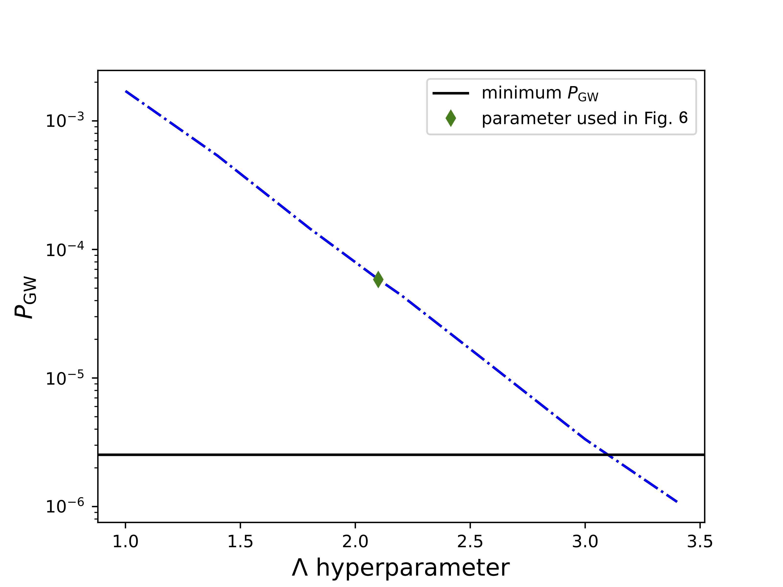
In Fig. 6, we show an exclusion plot of regions with $N_{\rm MSP}P_{\rm GW}>1$, using upper limits from the PowerFlux search. We note that each search has different sensitivity, covers different frequency ranges, and fixes different maximum $\dot{f}_{\rm GW}$, thus different searches would result in different exclusion regions on this plot. We show only PowerFlux results because they are the most constraining.

Figure 6: Constraints on the GeV excess for PowerFlux. The gray region is ruled out by this search for the chosen ellipticity and frequency PDFs. White regions are ruled out by Fermi-LAT. Here, $P_{\rm GW}=1/17000$.

Figure 7: One realization of the ellipticity PDF used to compute constraints on the GeV excess. We use 100 realizations of this PDF and average over the number of gravitational-wave signals we could have detected to arrive at the constraints in Fig. 6. The power law of this distribution is fixed to be $\Lambda=2.1$.

Note that $P_{\rm GW}$ is strongly sensitive to the value of $\Lambda$. In Fig. 8, we show this dependence, and in particular the smallest possible value of $\Lambda$ that would result in a constraint from PowerFlux in this search. $\Lambda$ controls the fall-off of the exponential distribution on ellipticities: smaller values indicate a slower fall-off, while larger values imply a quicker fall-off. Thus, for larger values of $\Lambda$, the constraints weaken, since there are fewer MSPs with larger ellipticities that would be more likely to be detected than those with smaller ellipticities.

Figure 8: Probability of detecting a gravitational-wave in the PowerFlux search as a function of the hyperparameter $\Lambda$. The horizontal line indicates the minimum $P_{\rm GW}$ at which a constraint would exist.

VI.3 Implications for light primordial black holes

Following the methodology outlined in section IV.3, for four different choices of $m_{1}$, we plot the upper limit on $\tilde{f}(m_{1},m_{2})$ as a function of $m_{2}$ in Fig. 9. Our results complement those that come from different searches of O3a [96, 97] and O4a data [6] that focus on shorter-duration, planetary-mass primordial black hole inspirals, and sub-solar mass searches (($[0.1,1]M_{\odot}$) [116, 105, 104, 23, 24, 106, 142]. Our limits are similar to those obtained in O3 [19], primarily because LIGO’s low-frequency sensitivity has not greatly improved from O3 to O4a. Since our constraining power primarily comes from low frequencies – where the frequency evolution of an inspiraling asteroid-mass system remains nearly monochromatic over the duration of O4a – our limits have not improved much with respect to the O3 search [19].

Figure 9: Constraint on $\tilde{f}$ from non-detection of asteroid-mass PBH binaries for PowerFlux. Codes to obtain these constraints are publicly available [99].

VII Summary and outlook

In summary, we have performed three independent all-sky searches for continuous gravitational waves, ranging from 20 Hz to as high as 2000 Hz, while probing spin-down magnitudes as high as $10^{-8}$ Hz/s. No credible gravitational wave signals are observed, allowing upper limits to be placed on possible signal amplitudes. Over a large fraction of the parameter space covered, these limits are the most stringent to date, with improvements in strain sensitivity due primarily to the improved noise floors of the LIGO interferometers over previous LIGO data sets. Fig. 2 shows the strain amplitude upper limits obtained from all three search pipelines, along with results from previous searches in O3 data.

The most stringent population-averaged strain upper limits reach $9.7\times 10^{-26}$ near 290 Hz, matching the best previous constraints up to $\sim$1700 Hz while extending coverage to a broader spin-down range. At higher frequencies, the new limits improve upon previous results by factors of approximately $\sim$1.6. At the highest frequencies ($\sim$2000 Hz) we are sensitive to neutron stars with an equatorial ellipticity $\epsilon$ as small as $\sim$$4\times 10^{-7}$ at distances as far away as $\sim$4.7 kpc. For ellipticities as high as $10^{-6}$, we are sensitive to neutron stars at the distance of the galactic center ($\sim$8.5 kpc).

The upper limits on strain amplitude from these searches have been interpreted in three specific astrophysical scenarios to constrain the populations of 1) galactic neutrons stars, 2) millisecond pulsars contributing to the GeV excess and 3) asteroid-scale primordial black holes.

Similar all-sky searches in the full O4 data ($>$2 year run) are expected to improve upon the sensitivities achieved for the $\sim$eight months analyzed here. Beyond the O4 run, significant improvements in detector noise are expected leading up to the fifth LIGO-Virgo-KAGRA run O5 planned for later in this decade. As search ranges extend to ever greater distances in the galaxy over ever broadening frequency sub-bands, the prospects for discovery should brighten [122, 109, 107].

VIII Acknowledgments

This material is based upon work supported by NSF’s LIGO Laboratory, which is a major facility fully funded by the National Science Foundation. The authors also gratefully acknowledge the support of the Science and Technology Facilities Council (STFC) of the United Kingdom, the Max-Planck-Society (MPS), and the State of Niedersachsen/Germany for support of the construction of Advanced LIGO and construction and operation of the GEO 600 detector. Additional support for Advanced LIGO was provided by the Australian Research Council. The authors gratefully acknowledge the Italian Istituto Nazionale di Fisica Nucleare (INFN), the French Centre National de la Recherche Scientifique (CNRS) and the Netherlands Organization for Scientific Research (NWO) for the construction and operation of the Virgo detector and the creation and support of the EGO consortium. The authors also gratefully acknowledge research support from these agencies as well as by the Council of Scientific and Industrial Research of India, the Department of Science and Technology, India, the Science & Engineering Research Board (SERB), India, the Ministry of Human Resource Development, India, the Spanish Agencia Estatal de Investigación (AEI), the Spanish Ministerio de Ciencia, Innovación y Universidades, the European Union NextGenerationEU/PRTR (PRTR-C17.I1), the ICSC - CentroNazionale di Ricerca in High Performance Computing, Big Data and Quantum Computing, funded by the European Union NextGenerationEU, the Comunitat Autonòma de les Illes Balears through the Conselleria d’Educació i Universitats, the Conselleria d’Innovació, Universitats, Ciència i Societat Digital de la Generalitat Valenciana and the CERCA Programme Generalitat de Catalunya, Spain, the Polish National Agency for Academic Exchange, the National Science Centre of Poland and the European Union - European Regional Development Fund; the Foundation for Polish Science (FNP), the Polish Ministry of Science and Higher Education, the Swiss National Science Foundation (SNSF), the Russian Science Foundation, the European Commission, the European Social Funds (ESF), the European Regional Development Funds (ERDF), the Royal Society, the Scottish Funding Council, the Scottish Universities Physics Alliance, the Hungarian Scientific Research Fund (OTKA), the French Lyon Institute of Origins (LIO), the Belgian Fonds de la Recherche Scientifique (FRS-FNRS), Actions de Recherche Concertées (ARC) and Fonds Wetenschappelijk Onderzoek - Vlaanderen (FWO), Belgium, the Paris Île-de-France Region, the National Research, Development and Innovation Office of Hungary (NKFIH), the National Research Foundation of Korea, the Natural Sciences and Engineering Research Council of Canada (NSERC), the Canadian Foundation for Innovation (CFI), the Brazilian Ministry of Science, Technology, and Innovations, the International Center for Theoretical Physics South American Institute for Fundamental Research (ICTP-SAIFR), the Research Grants Council of Hong Kong, the National Natural Science Foundation of China (NSFC), the Israel Science Foundation (ISF), the US-Israel Binational Science Fund (BSF), the Leverhulme Trust, the Research Corporation, the National Science and Technology Council (NSTC), Taiwan, the United States Department of Energy, and the Kavli Foundation. The authors gratefully acknowledge the support of the NSF, STFC, INFN and CNRS for provision of computational resources.

This work was supported by MEXT, the JSPS Leading-edge Research Infrastructure Program, JSPS Grant-in-Aid for Specially Promoted Research 26000005, JSPS Grant-in-Aid for Scientific Research on Innovative Areas 2402: 24103006, 24103005, and 2905: JP17H06358, JP17H06361 and JP17H06364, JSPS Core-to-Core Program A. Advanced Research Networks, JSPS Grants-in-Aid for Scientific Research (S) 17H06133 and 20H05639, JSPS Grant-in-Aid for Transformative Research Areas (A) 20A203: JP20H05854, the joint research program of the Institute for Cosmic Ray Research, University of Tokyo, the National Research Foundation (NRF), the Computing Infrastructure Project of the Global Science experimental Data hub Center (GSDC) at KISTI, the Korea Astronomy and Space Science Institute (KASI), the Ministry of Science and ICT (MSIT) in Korea, Academia Sinica (AS), the AS Grid Center (ASGC) and the National Science and Technology Council (NSTC) in Taiwan under grants including the Science Vanguard Research Program, the Advanced Technology Center (ATC) of NAOJ, and the Mechanical Engineering Center of KEK.

Additional acknowledgements for support of individual authors may be found in the following document:
https://dcc.ligo.org/LIGO-M2300033/public. For the purpose of open access, the authors have applied a Creative Commons Attribution (CC BY) license to any Author Accepted Manuscript version arising. We request that citations to this article use ’A. G. Abac et al. (LIGO-Virgo-KAGRA Collaboration), …’ or similar phrasing, depending on journal convention.

This document has been assigned LIGO Laboratory document number LIGO-P2500416-v6.

Appendix A Details concerning the PowerFlux search

We present in the following some details concerning the PowerFlux search.

A.1 PowerFlux search configuration

Table 7 gives the detailed configuration for the initial stage of the PowerFlux search, showing parameters that depend explicitly on coarse frequency bands.

	20-60 Hz	60-475 Hz	475-1475 Hz	1475-2000 Hz
Frequency bin width	0.139 mHz	0.139 mHz	0.278 mHz	0.556 mHz
Number of spin-down templates	220	110	33	110
Spin-down step size (Hz/s)	$5.0\times 10^{-11}$	$1.000\times 10^{-10}$	$3.333\times 10^{-10}$	$1.000\times 10^{-10}$
H1/L1 frequency mismatch tolerance (mHz)	2.5	2.5	2.5	2.5
H1/L1 spin-down mismatch tolerance (Hz/s)	$3.0\times 10^{-10}$	$3.0\times 10^{-10}$	$3.0\times 10^{-10}$	$3.0\times 10^{-10}$

Table 7: Information on the band-specific parameters for the initial search (stage 0) and outlier follow-up stages. The number of spin-down steps and the spin-down step size refer to the templates used in the stage-0 search. The tolerances refer to the consistency requirements between H1 and L1 outliers used to define candidates selected for stage-1 follow-up. Other search parameters relevant to all search bands are described in the text.

Stage	Instrument sum	Phase coherence $\delta$	Spin-down step	Sky refinement	Frequency refinement	SNR increase
		rad	Hz/s	$\alpha\times\delta_{0}$		%
20-60 Hz frequency range, 7200 s SFTs, 0.0625 Hz frequency bands
0	Initial/upper limit incoherent	NA	$5.0\times 10^{-11}$	$1$	$1/2$	–
1	incoherent	$\pi/2$	$2.5\times 10^{-11}$	$1/4\times 1/4$	$1/8$	10
2	coherent	$\pi/2$	$1.0\times 10^{-11}$	$1/4\times 1/4$	$1/8$	10
60-475 Hz frequency range, 7200 s SFTs, 0.0625 Hz frequency bands
0	Initial/upper limit incoherent	NA	$1.000\times 10^{-10}$	$1$	$1/2$	–
1	incoherent	$\pi/2$	$5.0\times 10^{-11}$	$1/4\times 1/4$	$1/8$	20
2	coherent	$\pi/2$	$1.0\times 10^{-11}$	$1/4\times 1/4$	$1/8$	10
475-1475 Hz frequency range, 3600 s SFTs, 0.125 Hz frequency bands
0	Initial/upper limit incoherent	NA	$3.333\times 10^{-10}$	$1$	$1/2$	–
1	incoherent	$\pi/2$	$1.0\times 10^{-10}$	$1/4\times 1/4$	$1/8$	20
2	coherent	$\pi/2$	$5.0\times 10^{-11}$	$1/4\times 1/4$	$1/8$	15
1475-2000 Hz frequency range, 1800 s SFTs, 0.25 Hz frequency bands
0	Initial/upper limit incoherent	NA	$1.000\times 10^{-10}$	$1$	$1/2$	–
1	incoherent	$\pi/2$	$3.0\times 10^{-11}$	$1/4\times 1/4$	$1/8$	20
2	coherent	$\pi/2$	$1.5\times 10^{-11}$	$1/4\times 1/4$	$1/8$	10

Table 8: PowerFlux outlier follow-up parameters. Stage 1 and higher use a loose-coherence algorithm for demodulation. The sky (both right ascension $\alpha$ and declination $\delta_{0}$) and frequency refinement parameters are relative to values used in the stage 0 PowerFlux search

The power calculation of the data can be expressed as a bilinear form of the input matrix $\left\{a_{t,f}\right\}$ constructed from the SFT coefficients with indices representing time and frequency:

$$P[f]=\sum_{t_{1},t_{2},D_{i},D_{j}}a_{t_{1},f+\Delta f(t_{1})}^{(D_{i})}a_{t_{2},f+\Delta f(t_{2})}^{(D_{j})*}K_{t_{1},t_{2},f}^{D_{i}D_{j}}\textrm{\penalty 10000\ .}$$ (14)

In this expression $\Delta f(t)$ is the detector-frame frequency drift due to the effects from both Doppler shifts and the first frequency derivative. The sum is taken over all times $t$ corresponding to the midpoints of the SFT time intervals. The kernel $K_{t_{1},t_{2},f}^{(D_{i}D_{j})}$ includes the contribution of time-dependent SFT noise weights, antenna response, signal polarization parameters, and relative phase terms [61, 62] for detectors $D_{i,j}$ (= H1, L1). Separate power sums are computed for H1, L1 and combined H1-L1 data.

The fast first-stage (stage 0) PowerFlux algorithm uses a kernel with diagonal terms only (including separate single-detector contributions $D_{i}=D_{j}$). The second stage (stage 1) increases effective coherence time while still allowing for controlled deviation in phase [61] via kernels that increase effective coherence length by inclusion of limited single-detector, off-diagonal terms. The third stage (stage 2) maintains the stage-1 effective coherence time, but adds SFT coefficients from H1 and L1 data coherently ($D_{i}\neq D_{j}$) to improve SNR and parameter resolution.

The effective coherence length is captured in a parameter $\delta$ [61], which describes the degree of phase drift allowed between SFTs. A value of $\delta=0$ corresponds to a fully coherent case, and $\delta=\pi$ corresponds to incoherent power sums.

Depending on the terms used, the data from different interferometers can be combined incoherently (such as in stages 0 and 1, see Table 8) or coherently (as used in stage 2). The coherent combination is more computationally expensive but improves parameter estimation.

A.2 Validation of the PowerFlux upper limits

Figure 10 shows results of a high-statistics “software injections” simulation run performed as described in [7]. Correctly established upper limits lie above the dashed diagonal lines (defining equality between upper limit obtained and true injection strain) in each panel, corresponding to four selected sub-bands [SFT coherence times]: 20-60 Hz [7200s], 60-475 Hz [7200s], 475-1475 Hz [3600s] and 1475-2000 Hz [1800s]. Performance for the 7200s-SFT 20-60 Hz and 60-475 Hz bands are shown separately because of the proliferation of spectral line artifacts below 60 Hz, primarily in the H1 data, and because of the large mismatch in H1 and L1 noise floors below $\sim$40 Hz. The breakpoint frequencies of 475 Hz and 1475 Hz for decreasing SFT coherence time are those used in the O1 PowerFlux search [13, 15], marking the starts of bands disturbed by 1st and 3rd violin mode harmonics. Additional band-specific parameters for the initial stage of the search are listed in Table 7.

Figure 10: Illustration of PowerFlux upper limit validation for very low, low, mid and high frequencies. Each point in the upper left, upper right, lower left and lower right panels represents a separate injection in the 20-60 Hz, 60-475 Hz, 475-1475 Hz and 1475-2000 Hz frequency ranges, respectively. Each established upper limit (vertical axis) is compared against the injected strain value defined by the horizontal axis (diagonal line defines equality of upper limit obtained and true injected strain).

A.3 Validation of the PowerFlux outlier follow-up

Testing of the stages 0–2 pipeline is performed for frequency bands searched via software injections using the same follow-up procedure. The recovery criteria also require that an outlier close to the true injection location (within 2.5 mHz in frequency $f$, $3\times 10^{-10}$ Hz/s in spin-down and 28.5 rad$\cdot$Hz$/f$ in sky location) be found and successfully pass through all stages of the detection pipeline.

Injection recovery efficiencies from simulations covering the major sub-bands (20-475 Hz, 475-1475 Hz, 1475-2000 Hz) are shown in Fig. 11 for stages 0, 1 and 2, which confirm that 95% signal recovery is comparable to the 95% upper limit in all bands, as desired, except for the region below 60 Hz for which spectral line artifacts heavily contaminate the H1 data set. Injections in vetoed frequency bands (see section III.2.2 and Table 9) are not included in these graphs.

Figure 11: Injection (software simulations) recovery efficiencies in the 20-60 Hz, 60-475 Hz, 475-1475 Hz and 1475-2000 Hz frequency bands are shown in the upper left, upper right, lower left and lower right panels, respectively, for stages 0, 1 and 2 of the search. The injected strain divided by the 95% CL upper limit in its band (without injection) is shown on the horizontal axis. The percentage of surviving injections is shown on the vertical axis, with a horizontal dashed line drawn at the $95$% level. The vertical dashed line marks a relative strain of unity. Ideally, the recovery efficiencies should lie to the left of the vertical line or above the horizonal line. One observes, however, that the ideal recovery efficiency is significantly degraded below 60 Hz, where large instrumental artifacts in the H1 data and only modest expected Doppler modulations make clean signal recovery more challenging. Most of the degradation stems from the band below 27 Hz for which H1 line contamination is severe and for which the H1 noise floor is substantially higher than the L1 noise floor.

A.4 Vetoed bands in the PowerFlux search

Table 9 shows particular frequency bands (about 13% of the original search band) for which no outlier follow-up is attempted for the initial or later stages because of instrumental artifacts that lead to such an unmanageable flood of initial or later-stage outliers.

Figure 12 shows the regions vetoed because of excessive outlier counts due to instrumental artifacts over the full search band, with a magnification of an example 100-Hz band (1900-2000 Hz) that includes a “forest” of 4th harmonics of violin modes from both interferometers.

$f_{\rm low}^{\rm veto}$	$f_{\rm high}^{\rm veto}$	$\Delta f^{\rm veto}$	$f_{\rm low}^{\rm veto}$	$f_{\rm high}^{\rm veto}$	$\Delta f^{\rm veto}$	$f_{\rm low}^{\rm veto}$	$f_{\rm high}^{\rm veto}$	$\Delta f^{\rm veto}$	$f_{\rm low}^{\rm veto}$	$f_{\rm high}^{\rm veto}$	$\Delta f^{\rm veto}$
(Hz)	(Hz)	(Hz)	(Hz)	(Hz)	(Hz)	(Hz)	(Hz)	(Hz)	(Hz)	(Hz)	(Hz)
27.097	27.903	0.805	301.720	302.580	0.860	898.260	900.940	2.680	1799.640	1800.310	0.670
27.247	27.613	0.365	302.870	303.630	0.761	906.059	907.141	1.081	1899.628	1900.316	0.688
27.332	27.673	0.341	305.819	306.581	0.761	909.459	910.541	1.082	1919.628	1920.372	0.744
27.547	27.883	0.336	307.119	307.881	0.761	918.458	919.142	0.684	1920.628	1921.372	0.744
27.707	28.073	0.366	314.619	315.482	0.863	922.308	923.022	0.715	1921.628	1922.372	0.744
28.047	28.393	0.346	410.100	410.500	0.400	958.724	959.296	0.572	1929.657	1932.843	3.186
29.807	30.133	0.326	416.673	417.064	0.390	959.724	960.276	0.552	1935.256	1937.894	2.637
32.017	32.653	0.636	419.379	419.767	0.388	960.724	961.276	0.552	1939.156	1941.394	2.238
33.178	33.488	0.310	419.558	420.442	0.884	986.751	1019.752	33.001	1947.255	1948.065	0.810
33.267	33.593	0.327	432.807	436.994	4.187	1022.248	1025.753	3.505	1948.755	1949.645	0.890
34.722	35.053	0.332	501.100	505.601	4.501	1224.797	1225.773	0.975	1952.155	1955.346	3.191
35.246	35.754	0.507	506.899	509.201	2.302	1229.997	1230.943	0.946	1952.605	1957.346	4.741
35.546	35.879	0.332	509.799	513.801	4.002	1259.424	1261.776	2.352	1957.654	1960.346	2.692
37.742	38.057	0.315	516.298	517.202	0.903	1463.704	1474.297	10.594	1960.054	1962.346	2.292
37.767	38.078	0.311	598.740	600.220	1.480	1480.702	1486.999	6.297	1961.654	1963.846	2.193
39.696	40.164	0.468	603.890	604.710	0.821	1489.201	1490.599	1.398	1964.154	1968.347	4.193
40.646	41.164	0.518	606.189	607.011	0.821	1491.201	1501.600	10.399	1967.453	1970.847	3.394
44.694	45.027	0.334	611.789	612.861	1.072	1509.919	1513.071	3.152	1971.203	1972.097	0.894
45.145	45.555	0.409	614.469	615.412	0.943	1511.999	1513.201	1.203	1977.652	1979.298	1.646
49.835	50.165	0.330	629.137	629.578	0.441	1599.660	1600.290	0.630	1980.152	1981.248	1.096
59.344	60.556	1.212	629.587	630.683	1.096	1699.650	1700.300	0.650	1981.212	1981.923	0.711
99.820	100.180	0.360	629.742	630.178	0.436	1729.617	1730.268	0.651	1984.851	1985.699	0.847
119.638	120.362	0.724	633.127	633.583	0.457	1737.901	1738.559	0.658	1985.301	1986.029	0.727
179.332	180.568	1.236	828.752	829.248	0.496	1745.375	1754.825	9.450	1987.951	1988.949	0.998
239.576	239.934	0.358	828.847	829.353	0.506	1797.835	1798.505	0.670	1993.451	1994.349	0.899
267.123	285.178	18.055	829.297	829.803	0.506	1798.870	1799.580	0.710	1993.951	1994.799	0.849
299.200	300.430	1.230	829.717	830.203	0.486	1799.450	1800.210	0.760	1999.610	2000.330	0.720

Table 9: Frequency bands vetoed from PowerFlux outlier follow-up because of excessive outlier counts from instrumental artifacts. The stage at which outlier followup is aborted is also shown for each band. Altogether, about 204 Hz out of the 1980-Hz original search band was vetoed, or about 10%.

Figure 12: Shaded regions (yellow) overlaid on the run-averaged spectra (inverse-noise weighted) from the H1 (red) and L1 (blue) O3a data sets indicate vetoed bands for which outlier follow-up is impeded by artifacts. The widest affected bands correspond to test-mass “violin modes” (ambient vibrations of the silica fibers from which LIGO mirrors are suspended) near multiples of 500 Hz. Top panel: Full 20-2000 Hz band. Bottom panel: Magnification of example 1900-2000 Hz band, for which line artifacts are dominated by the 4th harmonics of violin modes. (color online).

A.5 Upper limits results

Figure 13 presents strict PowerFlux upper limits on signals, for different assumed polarizations, along with PowerFlux upper limits from searches in the O3 data set [17, 135]. The cyan curve shows the upper limits for a worst-case (linear) polarization. The black curve shows upper limits for an optimally oriented source (circular polarization). Both curves represent strict frequentist upper limits on these worst-case and best-case orientations with respect to location on the sky, spin-down and frequency within each narrow search band. For sensitivity comparisons with other search pipeline results, the purple curve represents approximate population-averaged upper limits (over random sky locations and polarizations) and is derived from the circular polarization curve with a simple scale factor (2.3), based on injection studies in test bands.

Each linear-polarization or circular-polarization point in Fig. 13 represents a maximum over the sky, except for a small excluded portion of the sky near the ecliptic poles, which is highly susceptible to detector artifacts due to stationary frequency evolution produced by the combination of frequency derivative and Doppler shifts [7].

The O4a PowerFlux results presented here improve upon the previous O3a PowerFlux results in strain sensitivity with median factors ranging from $\sim$1.6 to $\sim$1.8 at signal frequencies above 300 Hz, where O4 detector noise improvement with respect to O3 performance is greatest.

Figure 13: PowerFlux upper limits on gravitational strain amplitude for this O4a analysis and for previous O3 analyses. The cyan curve shows worst-case (linearly polarized) O4a $95$% CL upper limits in analyzed ($62.5$ mHz, $125$ mHz, $250$ mHz) sub-bands for the broad (20-475 Hz, 475-1475 Hz, 1475-2000 Hz) search bands. The lowest black curve shows upper limits assuming a circularly polarized source. The dark blue curve shows approximate population-averaged all-sky upper limits inferred from the circularly polarized limits. For comparison, the red curve shows previous PowerFlux population-averaged 95% CL all-sky upper limits derived from the 6-month LIGO O3a data set [17], while the green curve extending up to 200 Hz shows population-averaged limits from a PowerFlux search of the full O3 data set [135], using loose coherence in the initial search stage.

Appendix B Details concerning the FrequencyHough search

We present in the following some details concerning the FrequencyHough search.

B.1 FrequencyHough method overview

We describe here the main analysis steps, with a particular emphasis on the new characteristics and to the specific choices used in this search. The first significant modification is that we have reorganized the FrequencyHough pipeline in order to make use of the BSD framework [117]. In fact, the use of band-limited time series of the detectors calibrated data, already down-sampled and cleaned, gives the opportunity to divide the analysis in steps of 1 Hz and therefore to evaluate Fast Fourier Transforms (FFTs) with duration $T_{\mathrm{FFT}}$ optimized for each 1 Hz band (the previous implementation used four different bands, each of fixed $T_{\mathrm{FFT}}$ duration). The condition [32] $T_{\mathrm{FFT}}<=\sqrt{\frac{c}{2\,f_{0}\,R_{0}}}/\Omega_{sid}$, where $f_{0}$ is the maximum frequency of the analysed band, $R_{0}$ the Earth radius at the detector location, $\Omega_{sid}$ the sidereal angular velocity, implies that the maximum Doppler effect (among all the possible sky positions) does not shift the frequency of the signal by more than one bin $\delta f=1/T_{\mathrm{FFT}}$. As a result, $T_{\mathrm{FFT}}$, in the first step of the search, ranges from 16384 s, at 20 Hz, to 1024 s at 1024 Hz, which is the highest frequency of the search, and is re-evaluated for each 1 Hz band (see Fig. 14). The cleaning is done before computing FFTs and consists in the identification of short time-domain disturbances with an autoregressive procedure and their subtraction from the data [35]. Next, local maxima above a given threshold are selected using the square root of the normalized power of the data, as done in previous searches. This collection of peaks is the so-called “peakmap”.

Figure 14: Comparison between the FrequencyHough $T_{\rm FFT}$ used in the O3 analysis [19] compared with the O4a one. We are able to fine-tune the coherence time thanks to the BSD framework [117].

As already mentioned in Sec. III.3, for each sky position the time-frequency peaks of the peakmap are properly shifted, to compensate for the Doppler effect due to the detector motion [36]. The shifted peaks are then fed to the FrequencyHough algorithm [36], which transforms each peak to the frequency/spin-down plane of the source. The frequency and spin-down bins (which we will refer to as coarse bins in the following) are defined, respectively, as $\delta f={1}/{T_{\mathrm{FFT}}}$ and $\delta\dot{f}={\delta f}/{T_{\textrm{obs}}}$, where $T_{\textrm{obs}}$ is the total run duration. In practice, the nominal frequency resolution has been increased by a factor of 10 [36], as FrequencyHough is not computationally bounded by the width of the frequency bin. The algorithm, moreover, adaptively weights any noise non-stationarity and the time-varying detector response [110]. In addition, in this search, a new - more computationally effective - implementation of the FrequencyHough algorithm has been used for the first time, described in Appendix B.2. The whole analysis is split into $\mathcal{O}$(millions) of independent jobs, each of which covers a small portion of the parameter space, see Appendix B.6. The output of a FrequencyHough   transform is a 2-D histogram in the frequency/spin-down plane of the source.

Outliers, that are statistically significant points in this plane, are selected by dividing each 1 Hz band of the corresponding histogram into 20 intervals and taking, for each interval and for each sky location, the one or (in most cases) the two outliers with the highest histogram number count [36], for each spin-down sub-range: $[-10^{-8},-7\times 10^{-9}]$ Hz/s, $[-7\times 10^{-9},\penalty 10000\ -4\times 10^{-9}]$ Hz/s, $[-4\times 10^{-9},\penalty 10000\ -1\times 10^{-9}]$ Hz/s, $[-1\times 10^{-9},\penalty 10000\ +2\times 10^{-9}]$ Hz/s. The second outlier is selected, as in previous searches, only if it is far enough from the highest one, suggesting the two have different origin. All the steps described so far are applied separately to the data of each detector involved in the analysis. As in past analyses [15, 16], coincidences among outliers of the two detectors are required, using a distance metric $d_{\rm FH}$ built in the four-dimensional parameter space of sky position $(\lambda,\penalty 10000\ \beta)$ (in ecliptic coordinates), frequency $f$ and spin-down $\dot{f}$. Thanks to some optimizations done in the entire analysis chain, we have been able to eliminate the clustering before coincidences, that was used in the past searches to reduce the computational load of making coincidences. Pairs of outliers with distance $d_{\rm FH}\leq 3$ are considered coincident.

Coincident outliers are ranked according to the value a statistic built using a combination of the distance and the FrequencyHough histogram weighted number count of the coincident outliers [36]. After the ranking, the eight outliers in each 0.01 Hz band (we have enhanced by a factor of 10 the number of selected outliers at this stage, for the same reasons stated above) with the highest values of the statistic are selected and subject to the follow-up.

B.2 New FrequencyHough implementation

The algorithm performing the FrequencyHough transform has been optimized with respect to the one used up through the O3 run. The FrequencyHough output map is a two-dimensional histogram over the frequency/spin-down parameter space in the source frame. In the previous implementation, each point in the input map was mapped as a straight line in the output space. Even if this mapping was implemented through a well-optimized loop, different points could write to the same memory locations, preventing this operation to be done in parallel. Following the inputs from [85] and under a flagship project inside ICSC [49], in the new implementation the loop has been inverted. Each point in the output map is computed by integrating along the corresponding line in the input map. This new implementation reaches the same performance as the previous one in terms of computing time when run on single-core CPUs. However, the new program can be executed in parallel exploiting modern parallel devices, in particular GPU devices, with a gain in speed of more than one order of magnitude in most cases.

B.3 FrequencyHough follow-up details

After the first follow-up step described in Sec. III.3.1, a sequence of vetoes is applied to refined outliers. First a new peakmap is created around the refined outlier frequency, using data corrected with updated parameters. This peakmap is projected onto the frequency axis and only those outliers whose Critical Ratio (CR) values have increased after the procedure are retained. The CR is defined as $CR=\frac{x-\mu}{\sigma}$, where $x$ is the value of the peakmap projection in a given frequency bin, $\mu$ is the average value and $\sigma$ the standard deviation of the projection. The projection is then analyzed by splitting the frequency range into sub-bands, and the outlier is kept only if it ranks among the top two peaks in both detectors. This significance veto is followed by a consistency check, which rejects coincident outliers whose CRs, properly weighted by the detector noise level, differ by more than a factor of five. To eliminate contamination from instrumental artifacts, outliers falling within known disturbed bands are also discarded. Additionally, coincident outlier pairs separated by a follow-up distance greater than a predefined threshold are excluded. Outliers associated with hardware injections are identified through similar criteria and analyzed separately for diagnostic purposes. Only those outliers that pass all these tests proceed to the subsequent follow-up stages, where the coherence time is further increased, and that are based on PyFstat [34, 84, 102] in a similar way to what is described in Sec. III.2. The second stage is run with $T_{\textrm{\mbox{\tiny{coh}}}}=0.5$ day [19, 18, 22, 21, 146, 20, 19]. We set Gaussian priors over $f$, $\dot{f}$, $\alpha$, $\delta$ following [102] where their standard deviation is set to the parameter’s resolutions. Additionally, we consider the second-order spin-down contribution for a set of outliers (see Sec. V.2.2) by including an additional Gaussian prior for this parameter.

Since PyFstat coherently combines H1 and L1 data, we center the priors at the average of the single-detector results of the previous stage. The MCMC configuration is set to the suggested one in [102]

$$N_{\mathrm{w}}=50,\,N_{\mathrm{t}}=1,\,N_{\mathrm{tot}}=300\,,$$

see [34] for more details on such parameters. The loudest template of the search is then taken as the follow-up stage’s output and compared with the noise distribution to estimate its false-alarm probability ($p_{\mathrm{fa}}$). Following the discussion in [102], we evaluated the $p_{\mathrm{fa}}$ for each outlier by running $500$ off-sourced MCMCs. In a similar manner to the suggested procedure of [133, 80], we performed the off-sourcing using the same priors of the search with only randomly shifting in each case the $\alpha$ value requiring that $\alpha-\alpha_{\rm cand}\geq\frac{\pi}{2}$ to avoid overlapping with the outlier’s parameter space. The loudest templates from all the runs are histogrammed and fitted with a Gumbel distribution similar to the procedure described in Appendix A of [102]. Only those outliers that fall below $p_{\mathrm{fa}}<1\%$ are deemed as outliers and checked carefully before being further analysed in a third follow-up stage. We examine the cumulative distribution of the detection statistic to discard outliers linked to detectors’ time-dependent instabilities, similarly to [19]. Outliers with sudden variations of the cumulative $2\mathcal{F}$ are discarded, while the others are followed up in another stage.

As a further check, we also compare the results from the MCMC stages using Eq. (11) of [19].

B.4 Inclusion of the second order spin-down

For the first time, we interpret the all-sky results in terms of an explicit spin-down power-law model for CW emission. Assuming that the source is spinning down following the power law, $\dot{f}\propto-f^{n}$ [144, 113], we can relate the expected second-order spin-down of the source to its frequency $f$ and $\dot{f}$ as

$$\ddot{f}=n\,\frac{\dot{f}^{2}}{f}\,,$$ (15)

where $n$ is the braking index of the NS, the value of which depends on the driving spin-down mechanism. For instance, $n=3$ for a NS losing rotational energy only through electromagnetic dipole emission and $n=5$ for a NS (sometimes referred to as gravitar) for which rotational energy is lost only through GWs. The current implementation of the FrequencyHough [36] and the first-stage follow-up procedure do not explicitly accommodate $\ddot{f}\neq 0$. We can identify the parameter-space region where the contribution of $\ddot{f}$ can be neglected by comparing Eq. eq:fddot_power_law with the natural resolution $\delta\!\ddot{f}=2\,\delta\!f/T_{\rm obs}^{2}$. When $\delta\!\ddot{f}>\ddot{f}$, then the search is not affected by the outlier’s second-order spin-down. For a gravitar, this condition is equivalent to

$$\dot{f}^{2}<\frac{2}{5}\,\frac{f_{0}}{T_{\rm FFT}\,T_{\rm obs}^{2}}\,.$$ (16)

Outliers with parameters such that Eq. eq:selection_gravitar_cands is verified at the first follow-up stage are analysed separately, including $\ddot{f}$ from the second follow-up stage on, where needed. This corresponds to outliers falling within the overlap between the blue and orange regions in Fig. 15. All the others have been analysed without accounting for any $\ddot{f}$ contribution.

Figure 15: Parameter space covered by the FrequencyHough in the O4a search (blue with diagonal hatching). The orange region with star hatching corresponds to the part of parameter space for which Eq. eq:selection_gravitar_cands is verified using the $T_{\mathrm{FFT}}$ of the first follow-up stage (three times that of the initial search, see Fig. 14). Here, the second stage of the follow-up, which is based on PyFstat and uses larger coherence times, has explicitly taken into account $\ddot{f}$ when needed. The portion of green region with vertical hatching not overlapped with the orange region denotes the part of parameter space for which Eq. eq:selection_gravitar_cands is verified using the $T_{\mathrm{FFT}}$ of the initial search, but not verified with the $T_{\mathrm{FFT}}$ of the first follow-up stage. The blue-only part of the parameter space corresponds to the situation in which Eq. eq:selection_gravitar_cands is never verified. All the follow-up stages in these two cases have been carried on without taking into account $\ddot{f}$.

B.5 FrequencyHough Sensitivity formula

The analytical formula for the search sensitivity, given by Eq. eq:hul, corrects an error in the original expression (equation 67 in [36]). The error was due to a wrong integrand in the inner integral in equation 19 of [36], where the probability of selecting a peak in presence of a signal of given amplitude was used, instead of the probability of selecting a peak in absence of signals. Using the correct integrand yields the following expression for the upper limit, at given confidence level $\Gamma$, averaged over all the source parameters: h_UL,Γ = 52π2.4308 S1/2nN1/4TFFT ×
(p0(1-p0)p12)^1/4 CR_max -2erfc^-1(2Γ), where

$$p_{0}=e^{-\theta}-e^{-2\theta}+\frac{1}{3}e^{-3\theta}$$ (17)

and

$$p1=\theta\left(\frac{1}{2}e^{-\theta}-\frac{1}{2}e^{-2\theta}+\frac{1}{6}e^{-3\theta}\right)+\frac{1}{4}e^{-2\theta}-\frac{1}{9}e^{-3\theta},$$ (18)

which differs from the expression originally found in [36]. Note also, in Eq. eq:hul, the absence of the term $\theta^{-1/2}$ present in equation 67 of [36]. Taking $\theta=2.5$ and the confidence level $\Gamma=0.95$ we obtain Eq. eq:hul. Numerically, the new expression gives estimated strain amplitude limits about 5$\%$ smaller than the original expression (for $\theta=2.5$). A more detailed discussion of the FrequencyHough analytical sensitivity estimation and of its various generalization is presented in [114].

B.6 FrequencyHough job submission framework

The computing workflow for the FrequencyHough search has been traditionally performed using storage and computing resources mainly provisioned by the INFN–CNAF Tier–1 [57] computing centre and strictly tied with its specific infrastructure. Starting with O4a, the workflow has been adapted to be more general and to also comply with computing centers in the IGWN [37] community. We tried to achieve a uniform submission framework which enables us to have the campaign progressing with different computing resource providers, such as the INFN–CNAF, the IGWN federation of sites, and possibly others, such as ICSC [49] or CINECA [136].

To pursue this objective several improvements or additions with respect to the previous model as adopted for O3, which was entirely performed at CNAF, were considered :

1. make the analysis code independent from site specific details, such as where the input files are located, how these should be accessed etc. The analysis code should start assuming that everything needed has been put in place already, and it should end assuming that the produced output will be properly handled and safely stored after it has done.

2. make every job behave as predictably as possible: in particular, the expected runtime of each job should be lower than the maximum allowed runtime at the site

3. whenever possible, recover and reuse partial results from evicted jobs

4. have the analysis campaign proceed in parallel over several distinct sites (such as CNAF) or network of sites (such as IGWN or ICSC)

5. have the computing campaign progress automatically, as unattended as possible

6. be resilient against paradigm shifts, such as protocol changes of some computing services. During the progress of the O4a analysis campaign, some auxiliary services muted their access interface and authentication method: CVMFS for data was deprecated and replaced by OSDF/Pelican, data access credentials shifted from X509 proxy to SCITOKENS etc. Impact on researcher’s code of these changes must be minimized at most, and the submission framework should be easily adaptable to comply with such changes.

The above items were addressed in chronological order and the resulting submission tool has been successfully adopted to complete the analysis for O4a as also a few more use cases. We plan to thoroughly describe this work in a dedicated document.

B.7 FrequencyHough upper limits from injections

In order to validate upper limits presented in Sec. V.2.2, several injections for each 1 Hz frequency band were done. We inject 100 signals in real data, with the same amplitude $h_{0}$, with parameters randomly drawn from those used in the real search. We compute the analysis on these new datasets and we count the number of signals that we are able to recover, meaning those that produce an outlier in the FrequencyHough maps, with a parameter space distance $\leq 3$ from one of the injections. This procedure is repeated for different amplitudes for each band, thus we obtain a curve of the fraction of signals recovered as a function of $h_{0}$. We hence perform a nonlinear fit using the three-parameters sigmoidal function:

$$f(x)=\frac{100\%}{\bigl(1+e^{-a(x-b)}\bigr)^{c}},$$ (19)

which is the Gompertz model. Here $a$ determines the steepness of the curve in the central region, and $b$ is a characteristic strain in that region (50% efficiency when $c=1$). The parameter $c$ takes into account potential asymmetries of the sigmoid, and it is 1 when the model Eq. eq:fh_gompertzmodel reduces to the logistic function. After this procedure, we are able to determine the 95% upper limit on signal strain. The whole procedure is repeated for 40 different frequency bands; in Fig. 16 we show an example of the fit for a specific band (95 Hz). In Fig. 17, we show the results obtained for all the bands where we computed upper limits with software injections. One sees that the theoretical estimation is a conservative choice.

Figure 16: Computation of $h_{0,\rm{min}}^{95\%}$ from FrequencyHough software injections for a specific frequency band (31 Hz). Blue points represent the fraction of signals recovered out of each 100-injections block. The red line and shaded region are the fit and its confidence interval. The green segment indicates the $h_{0,\rm{min}}^{95\%}$ estimation and its uncertainties.

Figure 17: Comparison between theoretical estimation of FrequencyHough upper limits (see Eq. eq:hul, blue curve) and its validation via software injections in some frequency bands (green points). The blue curve is obtained by taking the maximum outlier for each 1 Hz band. This estimation is conservative with respect to the limit obtained from injections.

Appendix C SOAP methodology

SOAP [42] is a fast, model-agnostic search for long duration signals based on the Viterbi algorithm [140].

C.0.1 Search pipeline

SOAP searches through each of the summed and narrow-banded spectrograms described in Sec. III.4.1 by rapidly identifying the track through the time frequency plane that gives the maximum sum of a detection statistic. In this search the statistic used is known as the ‘line aware’ statistic [42], which uses multiple detectors data to compute the Bayesian statistic $p(\rm{signal})/[p(\rm{noise})+p(\rm{line})]$, penalising instrumental line-like combinations of spectrogram powers. Since each of the four bands described in Sec. III.4.1 takes the sum of a different number of SFT bins, the $\chi^{2}$ distributions that make up the Bayesian statistic are adjusted such that they have $2\times N\times M$ degrees of freedom, where $M$ is the number of summed frequency bins and $N$ is the number of summed time segments.

SOAP then returns three main outputs for each sub-band: the Viterbi track, the Viterbi statistic and a Viterbi map. The Viterbi track is the time-frequency track which gives the maximum sum of statistics along the track, and is used for the parameter estimation stage in Sec. C.0.3. The Viterbi statistic is the sum of the individual statistics along the track, and is one of the measures used to determine the candidates for followup in Sec. III.4.3. The Viterbi map is a time-frequency map of the statistics in every time-frequency bin which has been normalised along every time step. This is representative of the probability distribution of the signal frequency conditional on the time step and is used as input to the convolutional networks described in Sec. C.0.2.

C.0.2 Convolutional neural network post processing

One post processing step in SOAP consists of CNNs which take in combinations of three data types: the Viterbi map, the two detectors’ spectrograms and the Viterbi statistic. The aim of this technique is to improve the sensitivity to isolated neutron stars by reducing the impact of instrumental artifacts on the detection statistic. This part of the analysis does add some model dependency, so is limited to search for signals that follow the standard CW frequency evolution. The structure of the networks is described in [40], where the output is a detection statistic which lies between 0 and 1. The networks are trained on $\sim 1\times 10^{5}$ examples of continuous wave signals injected into real data, where the data is split in the same way as described in Sec. III.4.1. Each of the sub-bands is duplicated, and a simulated continuous GW is injected into one of the two sub-bands such that the network has an example of noise and noise+signal cases. The sky positions, the frequency, frequency derivative, polarisation, cosine of the inclination angle and SNR of the injected signals are all uniformly drawn in the ranges described in [40]. These signals are then injected into real O4a data before the data processing steps described in Sec. III.4.1. As the neural network should not be trained and tested on the same data, each of the training sub-bands is split into two categories (‘odd’ and ‘even’), where the sub-bands are placed in these categories alternately such that an ’odd’ sub-band is adjacent to two ‘even’ sub-bands. This allows a network to be trained on ‘odd’ sub-bands and tested on ‘even’ sub-bands and vice-versa. The outputs from each of these networks can be combined and used as another detection statistic to be further analysed as described in Sec. III.4.3.

C.0.3 Parameter estimation

The parameter estimation stage uses the Viterbi track to estimate the Doppler parameters of the potential source. Because of the complicated and correlated noise which appears in the Viterbi tracks, defining a likelihood is challenging. To avoid this difficulty, likelihood-free methods are used, in particular a machine learning method known as a conditional variational auto-encoder. This technique was originally developed for parameter estimation of compact binary coalescence signals [65], and can return Bayesian posteriors rapidly ($<1$s). In our implementation, the conditional variational auto-encoder is trained on isolated NS signals injected into many sub-bands, and returns an estimate of the Bayesian posterior in the frequency, frequency derivative and sky position [41]. This acts both as a further check that the track is consistent with that of an isolated NS, and provides a smaller parameter space for a followup search.

March 15, 2026

The LIGO Scientific Collaboration, Virgo Collaboration, and KAGRA Collaboration

References

- [1] (2025-08) Einstein@Home all-sky ”bucket” search for continuous gravitational waves in LIGO O3 public data. Note: arXiv:2508.16423 External Links: 2508.16423 Cited by: §I, Figure 1, Figure 2, Figure 3, §V.4.
- [2] (2015-03) Advanced LIGO. Classical and Quantum Gravity 32 (7), pp. 074001. External Links: Document Cited by: §I.
- [3] (2016-02) First low frequency all-sky search for continuous gravitational wave signals. Phys. Rev. D 93, pp. 042007. External Links: Document Cited by: §III.3.
- [4] (2025-08) GWTC-4.0: Updating the Gravitational-Wave Transient Catalog with Observations from the First Part of the Fourth LIGO-Virgo-KAGRA Observing Run. Note: arXiv:2508.18082 External Links: 2508.18082 Cited by: §IV.3.
- [5] (2025-08) Open Data from LIGO, Virgo, and KAGRA through the First Part of the Fourth Observing Run. arXiv e-prints, pp. arXiv:2508.18079. External Links: Document, 2508.18079 Cited by: §II.
- [6] (2025-11) Search for planetary-mass ultra-compact binaries using data from the first part of the LIGO–Virgo–KAGRA fourth observing run. External Links: 2511.19911 Cited by: §VI.3.
- [7] (2012-01) All-sky search for periodic gravitational waves in the full S5 LIGO data. Physical Review D 85 (2), pp. 022001. External Links: ISSN 1550-2368, Document Cited by: §A.2, §A.5, §I, §III.2.1, §III.2, §III.2.
- [8] (2014) Astrophysical and Dark Matter Interpretations of Extended Gamma-Ray Emission from the Galactic Center. Phys. Rev. D 90 (2), pp. 023526. External Links: 1402.4090, Document Cited by: §IV.2.
- [9] (2011) The Consistency of Fermi-LAT Observations of the Galactic Center with a Millisecond Pulsar Population in the Central Stellar Cluster. JCAP 03, pp. 010. External Links: 1011.4275, Document Cited by: §IV.2.
- [10] (2008) All-sky search for periodic gravitational waves in LIGO S4 data. Phys. Rev. D 77, pp. 022001. Note: [Erratum: Phys.Rev.D 80, 129904 (2009)] External Links: 0708.3818, Document Cited by: §I, §III.1, §III.2, §III.2, §V.1.
- [11] (2009) All-sky LIGO Search for Periodic Gravitational Waves in the Early S5 Data. Phys. Rev. Lett. 102, pp. 111102. External Links: 0810.0283, Document Cited by: §I, §III.2.
- [12] (2016) Comprehensive all-sky search for periodic gravitational waves in the sixth science run LIGO data. Phys. Rev. D 94 (4), pp. 042002. External Links: 1605.03233, Document Cited by: §I, §III.2.
- [13] (2017) All-sky Search for Periodic Gravitational Waves in the O1 LIGO Data. Phys. Rev. D 96 (6), pp. 062002. External Links: 1707.02667, Document Cited by: §A.2, §I, §I, §III.2.1, §III.2.2, §III.2, §III.2.
- [14] (2017) First low-frequency Einstein@Home all-sky search for continuous gravitational waves in Advanced LIGO data. Phys. Rev. D 96 (12), pp. 122004. External Links: 1707.02669, Document Cited by: §I.
- [15] (2018) Full Band All-sky Search for Periodic Gravitational Waves in the O1 LIGO Data. Phys. Rev. D 97 (10), pp. 102003. External Links: 1802.05241, Document Cited by: §A.2, §B.1, §I, §I, §III.2.2, §III.2, §III.2, §III.3, §III.3.