Tensorial Reduced-Order Models for Parametric Coupled Reaction-Diffusion Systems: Application to Brain Tumor Growth Modeling

Abstract.

We construct efficient surrogate models for parametric forward operators arising in brain tumor growth simulations, governed by coupled semilinear parabolic reaction–diffusion systems on heterogeneous two- and three-dimensional domains. We consider two models of increasing complexity: a scalar single-species formulation and a six-state, nine-parameter multi-species go-or-grow model. The governing equations are discretized using a finite volume method and integrated in time via an operator-splitting strategy. We develop tensorial reduced-order model (TROM) surrogates based on the Higher-Order Singular Value Decomposition in Tucker format and the Tensor Train decomposition, each in intrusive and non-intrusive variants. The models are compared against a classical proper orthogonal decomposition (POD) ROM baseline. Numerical experiments with up to $m=9$ model parameters demonstrate speedups of $85\times$–$120\times$ relative to the full-order solver while maintaining excellent accuracy, establishing tensorial surrogates as a rigorous and efficient computational foundation for many-query workflows.

1. Introduction

Integrating simulation with optimization is a powerful paradigm for informed decision-making in biomedical applications [50, 9, 51]. Even the solution of the forward problem alone is often computationally demanding. In this work, we consider a coupled, nonlinear, time-dependent parameter-to-state map whose repeated evaluation becomes prohibitive in many-query settings such as inverse problems,statistical inference, and digital twin applications [23, 30, 73, 22, 81, 36].

To address this computational bottleneck, we investigate the construction of surrogate models based on different variants of reduced-order models (ROMs) of the discrete forward operator [8, 7, 29, 68, 1]. The underlying model consists of coupled semi-linear parabolic reaction–diffusion-type equations parameterized by an $m$-dimensional parameter vector $\theta\in\mathbb{R}^{m}$, posed on heterogeneous two- and three-dimensional domains. The state variables represent tumor cell populations, oxygen concentration, and tissue compartments, following established tumor growth modeling frameworks [70, 76, 50, 22].

Designing effective ROMs that accurately capture parametric and temporal variability in large-scale, time-dependent partial differential equations (PDEs) remains a significant challenge, particularly in high-dimensional parameter regimes [64]. In the present work, we demonstrate results for problems with parameter dimensions of up to $m=9$.

1.1. Outline of the Method

We consider coupled, parametric, semi-linear reaction–diffusion type PDE systems of the general form

$$\partial_{t}u(x,t)+\mathcal{L}(u,x,t;\theta)+\psi(u,x,t;\theta)=0$$

in $\Omega_{B}\times(0,1]$, $\Omega_{B}\subset\mathbb{R}^{d}$, $d\in\{2,3\}$, controlled by the model parameters $\theta\in\mathbb{R}^{m}$, with state variable $u:\Omega_{B}\times[0,1]\to\mathbb{R}_{+}^{n_{s}}$, initial condition $u(x,t=0)=u_{0}(x)$, and Neumann boundary conditions on $\partial\Omega_{B}$. Here, $\mathcal{L}$ is an inhomogeneous, linear diffusion operator and $\psi$ is a (typically non-linear) reaction term. We discretize this system using a finite volume method (FVM). For time integration, we consider first- and second-order accurate splitting schemes that treat the linear and non-linear terms individually. We consider several ROM variants to speed up the solution of the underlying PDE system. As a baseline, we use a proper orthogonal decomposition ROM (POD-ROM). In addition, we consider several variants of tensorial ROMs (TROMs) [46, 56, 60, 47, 67]. The first group of TROMs uses a higher-order singular value decomposition to construct the surrogate (HOSVD-TROM) [17]. The second group of TROMs uses a tensor-train decomposition (TT-ROM) [61].

1.2. Related Work

Works discussing tumor growth models of varying complexity are abundant in the literature, ranging from early reaction–diffusion formulations to multi-physics and multi-scale descriptions [77, 78, 28, 31, 33, 43, 57, 59, 34, 83, 58, 62]. In the present work, we consider a parametric, coupled system of semi-linear parabolic PDEs with six state variables representing tumor cell populations, oxygen concentrations, and tissue compartments. The interactions among these state variables are governed by nine parameters $\theta$. Variants of this model have been studied previously, for example in [70, 76, 50, 22]. Here, we do not account for mechanical coupling with the surrounding brain parenchyma; formulations that include such effects can be found in [30, 26, 31].

These types of models have been employed in a range of application-driven settings, including image analysis workflows [26, 71, 25, 51, 5, 4], treatmentplanning or design [43, 44, 69, 38, 82], and parameter estimation for prediction and decision support [22, 72, 73, 52, 30, 24, 84, 15, 55, 36]. These workflows typically require estimation of the model parameters $\theta$ from data, an aspect we do not address in the present work; instead, our focus is exclusively on the construction of efficient surrogate models for forward simulation.

Driven by substantial advances across applied mathematics, engineering, and computing hardware, there has been increasing interest in machine-learning-based surrogate models in recent years [55, 40, 85, 63, 80, 84, 14, 66, 45, 42]. We take a different, more mathematically grounded approach that provides rigorous approximation guarantees. In particular, we consider several ROM variants [8, 7, 29, 65]. Beyond such guarantees, projection-based ROMs offer further advantages over purely data-driven surrogates, including improved data efficiency, enhanced interpretability, certified error control, and predictable online computational complexity. Moreover, these approaches preserve a direct connection to the underlying governing equations, a property that is especially desirable in safety-critical and decision-support settings. A comprehensive overview of projection-based model reduction and hyper-reduction techniques can be found in [7].

The use of TROMs in the context of parabolic equations is not new [54, 18, 46, 48]. Tensorial and interpolatory reduction techniques can be understood as tools for recovering efficient offline/online decompositions in the presence of nonlinearities or nonaffine parameter dependence, particularly for problems exhibiting polynomial or multilinear structure [11]. In classical reduced-basis settings, such decompositions are readily available for affine operators, but become significantly more challenging once nonlinear terms are introduced. Hyper-reduction strategies, such as the empirical interpolation method and its discrete variant, address this issue by introducing additional approximation spaces for nonlinear operators [6, 12]. For problems with polynomial nonlinearities, tensorial variants of POD-ROM provide an alternative route to online efficiency by exploiting multilinear structure in the reduced operators, leading to reduced online costs that depend only on the reduced dimension [74]. In this sense, TROMs offer a natural framework for capturing parametric dependence while maintaining explicit control over computational complexity as the parameter dimension $m$ increases. We note that our numerical framework avoids certain difficulties associated with nonlinearities through the use of an operator-splitting strategy.

1.3. Contributions

We design and evaluate a numerical framework for the efficient surrogate-based simulation of brain tumor growth. Our major contributions are:

• We design an effective numerical framework for solving coupled, semi-linear reaction–diffusion type PDE systems arising in brain tumor growth modeling. The framework combines a finite volume discretization with an operator-splitting time integration strategy that separates linear diffusion from nonlinear reaction terms, enabling a straightforward and efficient deployment of projection-based surrogate models.

• We develop and compare four variants of tensorial reduced-order models: an interpolatory HOSVD-TROM and an interpolatory TT-ROM, each available in intrusive (projection-based) and non-intrusive implementations. These surrogates exploit the multilinear structure of the snapshot tensor to achieve simultaneous compression across spatial, temporal, and parameter dimensions.

• We introduce a spatial pre-compression stage that projects all snapshots onto a low-dimensional spatial subspace prior to tensor decomposition, rendering the offline construction tractable for large-scale three-dimensional problems.

• We provide a detailed empirical evaluation of the performance of the designed surrogate models for two brain tumor growth models of varying complexity—a scalar single-species and a six-state, nine-parameter multi-species formulation—in both two and three spatial dimensions.

• The proposed TROM surrogates deliver online speedups between $85\times$ and $120\times$ relative to the full-order solver while maintaining excellent approximation accuracy, significantly outperforming the POD-ROM baseline across all test cases considered.

1.4. Limitations

We identify several open issues and remaining research directions.

• Our methodology has been demonstrated for up to $m=9$ parameters; extending it to significantly higher parameter dimensions requires additional work, as the size of the training set grows exponentially with $m$ and the offline cost of constructing the snapshot tensor becomes rapidly prohibitive. To overcome this limitation, tensor completion and cross-approximation techniques have recently been studied in the context of TROM training [49, 10]; however, these approaches fall beyond the scope of the present paper.

• Our implementation is currently a research prototype written in MATLAB, which imposes practical limits on performance and scalability. Deploying the framework in a compiled, high-performance computing-ready language and exploiting parallelism in both the offline (snapshot generation) and online (tensor decomposition, reduced integration) stages is left to future work.

• The three-dimensional numerical experiments reported in this work are restricted to the single-species model; the multi-species formulation has only been validated in two spatial dimensions. Extending the multi-species model to three dimensions is an important next step but requires additional implementation effort and substantially larger computational resources for offline snapshot generation.

• The performance of the proposed surrogates in extrapolation regimes—i.e., for parameter values outside the training range $\Theta_{s}$—has not been systematically studied and remains an open question. This will become of particular importance for deploying the proposed methodology in the context of inference of parameter values from clinical data [50, 22, 52, 51, 24].

1.5. Outline

We present mathematical models in Section 2. This includes a single- and a multi-species model (see Section 2.1 and Section 2.2). We describe our numerical approach in Section 3. We describe the discretization in Section 3.1. We present our numerical time integration strategy in Section 3.2. We describe the designed surrogate models in Section 3.3. This includes a baseline POD-ROM (see Section 3.3.2), and four variants of TROMs—an HOSVD-TROM and a TT-ROM (see Section 3.3.3 and Section 3.3.4), each available in an intrusive and a non-intrusive implementation. We present numerical results in Section 4 and conclude with Section 5.

2. Mathematical Model

We present the mathematical models we are going to consider below. The first model considers a single-species semi-linear parabolic reaction–diffusion type model for the tumor cell density. The second model consists of a coupled system of a similar type that accounts for different cell phenotypes and nutrition.

2.1. Single Species Model

We model the tumor cell concentration $u(x,t)$ using the semi-linear parabolic PDE [53, 52, 24]

(1) $$\partial_{t}u(x,t)-\nabla\cdot\alpha(x)\nabla u(x,t)+\rho\,u(x,t)\left(1-u(x,t)\right) =0 \text{in}\,\,\Omega_{B}\times(0,1],$$

$$u(x,t) =u_{0}(x) \text{in}\,\,\Omega_{B}\times\{0\},$$

$$\partial_{n}u(x,t) =0 \text{in}\,\,\partial\Omega_{B}\times[0,1],$$

where $\Omega_{B}\subset\mathbb{R}^{d}$ denotes the domain occupied by brain parenchyma with boundary $\partial\Omega_{B}$ and closure $\bar{\Omega}_{B}$. The diffusion operator in 1 accounts for the migration of cells into surrounding (healthy) tissue. It is controlled by the scalar map $\alpha:\bar{\Omega}_{B}\to\mathbb{R}_{+}$. The third term in the equation is a non-linear logistic reaction operator that accounts for the proliferation of cells controlled by the proliferation rate $\rho>0$. The scalar field $\alpha$ is defined by

$$\alpha(x)\mathrel{\mathop{:}}=\alpha_{\textit{w}}\pi_{\textit{w}}(x)+\alpha_{\textit{g}}\pi_{\textit{g}}(x)=\alpha(\pi_{\textit{w}}(x)+(1/10)\pi_{\textit{g}}(x)),$$

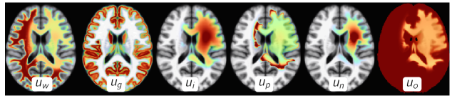
where $\pi_{\textit{w}}:\bar{\Omega}\to[0,1]$ and $\pi_{\textit{g}}:\bar{\Omega}\to[0,1]$ are white and gray matter probability maps obtained from a brain atlas so that $0\leq\pi_{\textit{w}}(x)+\pi_{\textit{g}}(x)\leq 1$ for all $x\in\Omega_{B}$ and $\pi_{\textit{w}}(x)=\pi_{\textit{g}}(x)=0$ for $x\in\Omega\setminus\Omega_{B}$. The migration into surrounding healthy tissue is controlled by the scalar parameters $\alpha_{w}=\alpha>0$ and $\alpha_{g}=\alpha/10>0$ (we simplify the model to be controlled by a single parameter $\alpha$).

2.2. Multi-Species Model

We extend the single-species formulation to a mathematical framework that captures the interplay between multiple tumor cell phenotypes, oxygen dynamics, and brain tissue heterogeneity. Similar formulations have been considered in [70, 76, 50, 22]. We do not include the mechanical coupling with linear elasticity equations, thereby neglecting tumor-induced mass effect.

The model is based on the go-or-grow hypothesis, which postulates that tumor cells switch between two primary phenotypes: proliferative, denoted by $u_{\textit{p}}:\bar{\Omega}_{B}\times[0,1]\to\mathbb{R}_{+}$, and infiltrative, denoted by $u_{\textit{i}}:\bar{\Omega}_{B}\times[0,1]\to\mathbb{R}_{+}$. In nutrient-rich and oxygenated regions, proliferative cells undergo rapid mitosis, driving local tumor expansion. Under hypoxic conditions, cells transition to the infiltrative phenotype, enabling migration toward better-oxygenated regions. Upon encountering favorable conditions, infiltrative cells revert to the proliferative phenotype, continuing the growth–migration cycle. Severe hypoxia leads to cell death and the formation of a necrotic core, denoted by $u_{\textit{n}}$. Oxygen concentration, denoted by $u_{\textit{o}}:\bar{\Omega}_{B}\to\mathbb{R}_{+}$, plays a central regulatory role, influencing both proliferation rates and phenotypic switching. The oxygen field is consumed by tumor cells and supplied by healthy vasculature, with rates $\kappa_{c}\geq 0$ and $\kappa_{s}\geq 0$, respectively. Gray matter, denoted by $u_{\textit{g}}:\bar{\Omega}_{B}\to\mathbb{R}_{+}$, and white matter, $u_{\textit{w}}:\bar{\Omega}_{B}\to\mathbb{R}_{+}$, fractions contribute to the spatially varying diffusion coefficient $\alpha:\bar{\Omega}\to\mathbb{R}_{+}$ and proliferation rate $\rho:\bar{\Omega}\to\mathbb{R}_{+}$. These tissue maps remain fixed in time and satisfy $u_{\textit{g}}+u_{\textit{w}}=u_{\textit{h}}$, where $u_{\textit{h}}$ denotes the healthy tissue.

Overall, we model the evolution of the densities $u:\bar{\Omega}_{B}\times[0,1]\to\mathbb{R}^{n_{s}}_{+}$, with $n_{s}=6$,

$$(x,t)\mapsto u(x,t)=(u_{\textit{p}},u_{\textit{i}},u_{\textit{n}},u_{\textit{o}},u_{\textit{g}},u_{\textit{w}})(x,t),$$

as the following coupled, semi-linear system of parabolic PDEs defined in $\Omega_{B}\times(0,1]$:

(2a) $$\partial_{t}u_{\textit{p}}-f(u_{\textit{p}})+\gamma_{p}^{u}u_{\textit{p}}(1-u_{\textit{i}})-\gamma_{i}^{u}u_{\textit{i}}(1-u_{\textit{p}})+\nu_{o}^{u}u_{\textit{p}}(1-u_{\textit{n}}) =0,$$

(2b) $$\partial_{t}u_{\textit{i}}-\nabla\cdot\alpha\nabla u_{\textit{i}}-f(u_{\textit{i}})+\gamma_{i}^{u}u_{\textit{i}}(1-u_{\textit{p}})-\gamma_{p}^{u}u_{\textit{p}}(1-u_{\textit{i}})+\nu_{o}^{u}u_{\textit{i}}(1-u_{\textit{n}}) =0,$$

(2c) $$\partial_{t}u_{\textit{n}}-\nu_{o}^{u}(u_{\textit{i}}+u_{\textit{p}})(1-u_{\textit{n}}) =0,$$

(2d) $$\partial_{t}u_{\textit{o}}+\kappa_{c}u_{\textit{o}}u_{\textit{p}}-\kappa_{s}(1-u_{\textit{o}})(u_{\textit{w}}+u_{\textit{g}}) =0,$$

(2e) $$\partial_{t}u_{\textit{w}}+(u_{\textit{w}}/(u_{\textit{w}}+u_{\textit{g}}))\left(\nabla\cdot\alpha^{u}\nabla u_{\textit{i}}+f(u_{\textit{p}})+f(u_{\textit{i}})\right) =0,$$

(2f) $$\partial_{t}u_{\textit{g}}+(u_{\textit{g}}/(u_{\textit{w}}+u_{\textit{g}}))\left(\nabla\cdot\alpha^{u}\nabla u_{\textit{i}}+f(u_{\textit{p}})+f(u_{\textit{i}})\right) =0,$$

with initial conditions $u_{\textit{p}}=u_{\textit{p}}^{0}$, $u_{\textit{i}}^{0}=0$, $u_{\textit{n}}^{0}=0$, $u_{\textit{o}}^{0}=1$, $u_{\textit{w}}=u_{\textit{w}}^{0}$ and $u_{\textit{g}}=u_{\textit{g}}^{0}$ in $\Omega_{B}\times\{0\}$ and Neumann boundary conditions in $\partial\Omega_{B}\times[0,1]$. Here, the equations 2a, 2b, 2c model the evolution of proliferative tumor cells $u_{\textit{p}}$, infiltrative tumor cells $u_{\textit{i}}$, and necrotic tumor cells $u_{\textit{n}}$. Equation 2d accounts for the temporal evolution of the oxygen concentration $u_{\textit{o}}$. The last two equations 2e and 2f model the change of the healthy tissue $u_{\textit{g}}$ (gray matter) and $u_{\textit{w}}$ (white matter) attributed to infiltrating and proliferating tumor cells. We summarize the fields that appear in 2 in Table 1.

Table 1. List of variables and parameter maps used in the multispecies go-or-grow tumor model. This table summarizes the notation used for the tumor cell populations, oxygen dynamics, and transition rates between proliferative and infiltrative phenotypes. The model is based on [24, 70, 76, 22].

symbol	description	equation
$u_{\textit{p}}(x,t)$	density of proliferative tumor cells	2a
$u_{\textit{i}}(x,t)$	density of infiltrative tumor cells	2b
$u_{\textit{n}}(x,t)$	density of necrotic tumor cells	2c
$u_{\textit{o}}(x,t)$	oxygen concentration in the tumor micro-environment	2d
$u_{\textit{g}}(x,t)$	density of gray matter cells	2f
$u_{\textit{w}}(x,t)$	density of white matter cells	2e
$\alpha(x,t)$	diffusion coefficient map	3
$f(u)$	net reaction term modeling tumor proliferation	4
$\rho^{u}(x,t)$	proliferation rate	5
$\gamma_{p}^{u}(x,t)$	transition rate for proliferative to infiltrative phenotype	7a
$\gamma_{i}^{u}(x,t)$	transition rate for infiltrative to proliferative phenotype	7b
$\nu_{o}^{u}(x,t)$	oxygen-dependent transition threshold	6

The model in 2 is controlled by various parameters. We summarize these parameters in Table 2. We introduce a superscript $u$ if the value of the parameter depends on the species that appear in our model. In the following, we derive principled rules for computing these parameters and introduce suitable simplifications to reduce the size of the parameter space, with a view toward its use in an inverse problem.

The field $\alpha^{u}:\bar{\Omega}_{B}\to\mathbb{R}_{+}$ that appears in 2e and 2f controls the infiltration of $u_{\textit{i}}$ into surrounding healthy tissue. We assume that infiltration is different in white matter than in gray matter. The model for $\alpha$ is given by

(3) $$\alpha^{u}(x,t)=\alpha_{w}u_{\textit{w}}(x,t)+\alpha_{g}u_{\textit{g}}(x,t)=\alpha(u_{\textit{w}}(x,t)+(1/5)u_{\textit{g}}(x,t))$$

with parameters $\alpha_{w}=\alpha>0$ and $\alpha_{g}=(\alpha/5)>0$ (we reduce the model to be controlled by a single parameter $\alpha>0$).

The net reaction term $f$ that appears in 2a, 2b, 2d, respectively, accounts for logistic proliferation modulated by oxygen availability. The model is controlled by the proliferation rate $\rho^{u}:\bar{\Omega}_{B}\times[0,1]\to\mathbb{R}_{+}$, and the thresholds $u_{\textit{o}}^{\textit{inv}}>0$, $u_{\textit{o}}^{\textit{mit}}>0$, and $u_{\textit{o}}^{\textit{hyp}}>0$ for invasion, mitosis, and hypoxia, where $u_{\textit{o}}^{\textit{mit}}=(u_{\textit{o}}^{\textit{hyp}}+u_{\textit{o}}^{\text{inv}})/2$. Let $u_{\textit{s}}(x,t)=u_{\textit{p}}(x,t)+u_{\textit{i}}(x,t)+u_{\textit{n}}(x,t)$ for all $t\in[0,1]$, $x\in\Omega_{B}$, with $0\leq u_{\textit{s}}\leq 1$. Then, for some concentration $\tilde{u}(x,t)$, we have

(4) $$f(\tilde{u})(x,t)=\begin{cases}\rho^{\tilde{u}}(x,t)\tilde{u}(x,t)(1-u_{\textit{s}}(x,t))&\text{for}\,\,u_{\textit{o}}>u_{\textit{o}}^{\textit{inv}},\\ \rho^{\tilde{u}}(x,t)\tilde{u}(x,t)(1-u_{\textit{s}}(x,t))\dfrac{u_{\textit{o}}-u_{\textit{o}}^{\textit{mit}}}{u_{\textit{o}}^{\textit{inv}}-u_{\textit{o}}^{\textit{mit}}}&\text{for}\,\,u_{\textit{o}}^{\textit{inv}}\geq u_{\textit{o}}\geq u_{\textit{o}}^{\textit{mit}},\\ 0&\text{for}\,\,u_{\textit{o}}<u_{\textit{o}}^{\textit{mit}}.\end{cases}$$

The factor $(1-u_{\textit{s}}(x,t))$ ensures that there will be no reaction or increase of tumor concentration once the total tumor concentration $u_{\textit{s}}\approx 1$. We model $\rho^{u}$ as

(5) $$\rho^{\tilde{u}}(x,t)=\rho_{w}^{\tilde{u}}u_{\textit{w}}(x,t)+\rho_{g}^{\tilde{u}}u_{\textit{g}}(x,t)$$

controlled by the parameters $\rho_{g}^{\tilde{u}}>0$ and $\rho_{w}^{\tilde{u}}>0$. These parameters depend on the species $u$. To reduce the dimension of our parameter space, we collapse the model to be controlled by a single parameter $\rho>0$. For $u_{\textit{p}}$ we set

$$\rho^{u_{\textit{p}}}(x,t)=\rho(u_{\textit{w}}(x,t)+(1/5)u_{\textit{g}}(x,t)),$$

i.e., $\rho_{w}^{u_{\textit{p}}}=\rho$ and $\rho_{g}^{u_{\textit{p}}}=\rho/5$. Likewise, for $u_{\textit{i}}$ we choose

$$\rho^{u_{\textit{i}}}(x,t)=(\rho/10)(u_{\textit{w}}(x,t)+(1/5)u_{\textit{g}}(x,t)),$$

i.e., $\rho_{w}^{u_{\textit{i}}}=\rho/10$ and $\rho_{g}^{u_{\textit{i}}}=\rho/50$.

Oxygen-dependent cell death is controlled by the parameter $\nu_{o}^{u}$. This parameter appears in 2a, 2b, 2c. We model it as

(6) $$\nu_{o}^{u}(x,t)=\lambda_{d}h_{\varepsilon}(u_{\textit{o}}^{\textit{hyp}}-u_{\textit{o}}(x,t)),$$

where $h_{\varepsilon}(x)=1/(1+\exp(-x/\varepsilon))$ is a smooth approximation of the Heaviside function, where $\varepsilon>0$ controls the smoothness of the transition and $\lambda_{d}>0$ is the death rate of the tumor cells.

The switching between phenotypes $u_{\textit{i}}$ and $u_{\textit{p}}$ is controlled by the transition parameters $\gamma_{p}^{u}$ and $\gamma_{i}^{u}$ that appear in 2a and 2b. We model the rates according to

(7a) $$\gamma_{p}^{u} =\gamma_{p}h_{\varepsilon}(u_{\textit{o}}^{\textit{inv}}-u_{\textit{o}}),$$

(7b) $$\gamma_{i}^{u} =\gamma_{i}h_{\varepsilon}(u_{\textit{o}}-u_{\textit{o}}^{\textit{inv}}),$$

controlled by the scalar parameters $\gamma_{p}>0$ and $\gamma_{i}>0$. The remaining user defined parameters are $\kappa_{s}>0$ (the oxygen supply rate) and $\kappa_{c}>0$ (the oxygen consumption rate); they appear in 2d. In summary, based on the simplifications that allowed us to reduce the dimension of the parameter space $\Theta\subset\mathbb{R}^{m}_{+}$, the considered model is controlled by the following $m=9$ parameters

$$\theta=(\alpha,\rho,\gamma_{p},\gamma_{i},\lambda_{d},\kappa_{s},\kappa_{c},u_{\textit{o}}^{\textit{inv}},u_{\textit{o}}^{\textit{hyp}})\in\Theta.$$

We summarize these parameters, their meaning, and values and parameter ranges considered in the literature in Table 2.

Table 2. Model parameters, values, and parameter ranges for the system 2. The parameters correspond to reaction and diffusion coefficients, go-or-grow transition rates, oxygen dynamics, and screening properties of the model considered and developed in [70, 76, 22]. The values included here are based on [24, 70]. Derived values are highlighted in gray.

symbol	description	default value	range	equation
$\alpha$	diffusion coefficient	$0.05$	[$1\text{\times}{10}^{-3}$, $1\text{\times}{10}^{-1}$]	3
gray!40$\alpha_{w}$	diffusion coefficient in white matter	$\alpha$
gray!40$\alpha_{g}$	diffusion coefficient in gray matter	$0.2\alpha=0.01$
$\rho$	reaction coefficient	$18.0$	[$5.0$, $2.5\text{\times}{10}^{1}$]	5
gray!40$\rho_{w}^{u_{\textit{p}}}$	reaction coefficient in white matter	$\rho$
gray!40$\rho_{g}^{u_{\textit{p}}}$	reaction coefficient in gray matter	$0.2\rho=3.6$
gray!40$\rho_{w}^{u_{\textit{i}}}$	reaction coefficient in white matter	$0.1\rho=1.8$
gray!40$\rho_{g}^{u_{\textit{i}}}$	reaction coefficient in gray matter	$0.02\rho=0.36$
$\gamma_{p}$	transition rate from $u_{\textit{p}}$ to $u_{\textit{i}}$	$5.0$	[$1\text{\times}{10}^{-1}$, $1.0\text{\times}{10}^{1}$]	7a
$\gamma_{i}$	transition rate from $u_{\textit{i}}$ to $u_{\textit{p}}$	$7.0$	[$1\text{\times}{10}^{-1}$, $1.5\text{\times}{10}^{1}$]	7b
$\lambda_{d}$	death rate	$10.0$	[$1.0$, $2.0\text{\times}{10}^{1}$]	6
$u_{\textit{o}}^{\textit{hyp}}$	hypoxia oxygen threshold	$0.5$	[$1\text{\times}{10}^{-3}$, $6\text{\times}{10}^{-1}$]	6
$u_{\textit{o}}^{\textit{inv}}$	invasive oxygen threshold	$0.90$	[$7\text{\times}{10}^{-1}$, $1.0$]	7a,7b
$\kappa_{s}$	oxygen supply rate	$6$	[$1.0$, $8.0$]	2d
$\kappa_{c}$	oxygen consumption rate	$15.0$	[$1.0$, $2.0\text{\times}{10}^{1}$]	2d

3. Numerical Methods

In this section, we introduce a numerical approach for solving the dynamical systems 1 and 2. For simplicity of presentation, we develop the methodology using the prototypical equation,

(8) $$\partial_{t}u(x,t)-\nabla\cdot\alpha(x)\nabla u(x,t)+\psi(u,x,t)=0\quad\text{in}\quad\Omega_{B}\times(0,1]$$

with initial condition $u(x,t)=u_{0}(x)$ in $\Omega_{B}\times\{0\}$ and Neumann’s boundary conditions $\partial_{n}u(x,t)=0$ in $\partial\Omega_{B}\times[0,1]$. This equation allows us to consolidate 1 and 2 into a single model; the relation to 1 is straightforward; for 2, we can assume with a slight abuse of notation that $u(x,t)=(u_{\textit{p}},u_{\textit{i}},u_{\textit{n}},u_{\textit{o}},u_{\textit{g}},u_{\textit{w}})(x,t)$. To keep the notation light, we mostly limit the description of the numerical approach to a single species model. For the ROMs considered in our work, we construct reduced models for each species as outlined below.

3.1. Numerical Discretization

We discretize the equations using a finite volume method [19, 41]. Our discretization strategy follows [53]. Let $d\in\{1,2,3\}$ denote the dimension of the ambient space. We discretize the function $u:\bar{\Omega}\to\mathbb{R}$ with $\Omega\mathrel{\mathop{:}}=[\omega_{1},\omega_{2}]\times\cdots\times[\omega_{2d-1},\omega_{2d}]\subset\mathbb{R}^{d}$ on a cell centered grid $\Omega^{h}\in\mathbb{R}^{d\times n_{1}\times\cdots\times n_{d}}$, where $n_{i}\in\mathbb{N}$ denotes the number of cells. The grid coordinates $x_{k}=(x_{k}^{1},\ldots,x_{k}^{d})\in\mathbb{R}^{d}$, $k\in\mathbb{Z}^{d}$, with $x_{k}^{i}=\omega_{2i-1}+(k_{i}-1/2)h_{i}$ represent the center point of a cell of width $h=(h_{1},\ldots,h_{d})\in\mathbb{R}^{d}$, $h_{i}=(\omega_{2i}-\omega_{2i-1})/n_{i}$. Similarly, we discretize the temporal domain $[0,1]$ using a nodal mesh consisting of $n_{t}+1$ time points with mesh size $h_{t}=1/n_{t}$ and time points $t^{j}=(j-1)h_{t}$. Consequently, the numerical approximation of $u$ at location $x_{k}$ and time point $t^{j}$ is given by $u_{k}^{j}\approx u(x_{k},t^{j})$. We arrange the discrete $u_{k}^{j}$ in lexicographical ordering to obtain

$$u^{j}_{h}=(u_{1,\ldots,1}^{j},\ldots,u_{n_{1},\ldots,n_{d}}^{j})\in\mathbb{R}^{n_{x}},$$

where $n_{x}=\prod_{i=1}^{d}n_{i}$ denotes the total number of mesh points.

Before we introduce our scheme for integrating the equation in time, we are going to discuss the discretization in space. As such, we will work with the semi-discrete state variable

$$u_{h}(t)=(u_{1,\ldots,1}(t),\ldots,u_{n_{1},\ldots,n_{d}}(t))\in\mathbb{R}^{n_{x}}.$$

We use short differences to discretize the gradient operator. We obtain the sparse matrix

$$G_{i}=\frac{1}{h^{i}}\begin{pmatrix}b_{1}&b_{2}&&&&\\ &-1&1&&&\\ &&\ddots&\ddots&&\\ &&&-1&1&\\ &&&&b_{3}&b_{4}\\ \end{pmatrix}\in\mathbb{R}^{n_{i}+1\times n_{i}}$$

for the $i$th coordinate direction; $b_{j}$ represent the entries for the boundary conditions. The two and three-dimensional gradient operators are constructed using Kronecker products; we have

$$\operatorname{GRAD}=\begin{pmatrix}I_{n_{1}}\otimes G_{1}\\ G_{2}\otimes I_{n_{2}}\end{pmatrix}\in\mathbb{R}^{(n_{1}+1)n_{2}+(n_{2}+1)n_{1}\times n_{1}n_{2}}$$

for $d=2$ and

$$\operatorname{GRAD}=\begin{pmatrix}I_{n_{3}}\otimes I_{n_{2}}\otimes G_{1}\\ I_{n_{3}}\otimes G_{2}\otimes I_{n_{1}}\\ G_{3}\otimes I_{n_{2}}\otimes I_{n_{1}}\\ \end{pmatrix}\in\mathbb{R}^{\tilde{n}\times n_{1}n_{2}n_{3}}$$

with $\tilde{n}=(n_{1}+1)n_{2}n_{3}+n_{1}(n_{2}+1)n_{3}+n_{1}n_{2}(n_{3}+1)$. Notice that for $d=1$, $\operatorname{GRAD}$ maps from a cell-centered grid to a nodal grid. For $d=2$ and $d=3$, $\operatorname{GRAD}$ maps from a cell-centered grid to a staggered grid.

The divergence operator is given by

$$\operatorname{DIV}=\begin{pmatrix}I_{n_{1}}\otimes G_{1}&G_{2}\otimes I_{n_{2}}\end{pmatrix}\in\mathbb{R}^{n_{1}n_{2}\times(n_{1}+1)n_{2}+(n_{2}+1)n_{1}}$$

for $d=2$ and

$$\operatorname{DIV}=\begin{pmatrix}I_{n_{3}}\otimes I_{n_{2}}\otimes G_{1}&I_{n_{3}}\otimes G_{2}\otimes I_{n_{1}}&G_{3}\otimes I_{n_{2}}\otimes I_{n_{1}}\end{pmatrix}\in\mathbb{R}^{n_{1}n_{2}n_{3}\times\tilde{n}}$$

for $d=3$. The operator $\operatorname{DIV}$ maps back to the original cell-centered grid.

We assume that the coefficient map $\alpha$ is also allocated on a cell-centered grid. To map $\alpha_{h}\in\mathbb{R}^{n_{x}}$ to a staggered grid, we introduce the one-dimensional grid change operator

$$M_{i}=\frac{1}{2}\begin{pmatrix}3&-1&&\\ 1&1&&\\ &\ddots&\ddots&\\ &&1&1\\ &&-1&3\\ \end{pmatrix}\in\mathbb{R}^{n_{i}+1\times n_{i}}.$$

The $d$-dimensional operator $\operatorname{AVG}$ is constructed with the same stencil as $\operatorname{GRAD}$. Using these matrices, we can approximate the diffusion operator $\mathcal{L}(\alpha)=-\nabla\cdot\alpha(x)\nabla$ as

$$L_{h}\mathrel{\mathop{:}}=-\operatorname{DIV}\operatorname{diag}(e\oslash(\operatorname{AVG}\alpha_{h}))\operatorname{GRAD}\in\mathbb{R}^{n_{x}\times n_{x}},$$

where $e=\begin{pmatrix}1,\ldots,1\end{pmatrix}\in\mathbb{R}^{\tilde{n}}$, $\oslash:\mathbb{R}^{\tilde{n}}\to\mathbb{R}^{\tilde{n}}$ denotes element-wise division (Hadamard division) and $e\oslash(\operatorname{AVG}\alpha_{h})$ implements harmonic averaging.

The discretization of $\psi$ is straightforward; for example, for $\psi(u,x,t)=\rho u(x,t)(1-u(x,t))$, we obtain the semi-discrete expression

$$\psi_{h}(u_{h}(t),t)=\rho u_{h}(t)\odot(e-u_{h}(t))\in\mathbb{R}^{n_{x}}.$$

Overall, we arrive at the semi-discrete system of ODEs

(9) $$\text{d}_{t}u_{h}(t)=f_{h}(u_{h}(t),t)$$

with $f_{h}(u_{h}(t),t)\mathrel{\mathop{:}}=L_{h}u_{h}(t)-\psi_{h}(u_{h}(t),t)$.

One issue we have not addressed so far is that we actually need to implement these operators on a non-rectangular, complex domain $\Omega_{B}$ with a curved boundary $\partial\Omega_{B}$. For this purpose, we use a fictitious domain method to implement the boundary conditions [52, 53, 30].

3.2. Numerical Time Integration

Our approach for integrating 8 in time follows ideas presented in [70, 76, 24]. We consider a second order accurate Strang operator splitting scheme in the present work (cf., e.g., [75, 32]), splitting the equation into diffusion and reaction steps; see Algorithm 1.

Algorithm 1 Second order accurate Strang splitting. We solve the diffusion step using a Crank–Nicolson method. The reaction step is solved analytically or numerically (using a second-order Runge–Kutta method).

1:$\hat{u}_{h}\leftarrow$ solve $(I_{n_{x}}-(h_{t}/4)L)\hat{u}_{h}=(I_{n_{x}}+(h_{t}/4)L)u^{j}_{h}$

2:$\tilde{u}_{h}\leftarrow$ solve $\partial_{t}u=-\psi(u,x,t)$ in $[t^{j},t^{j+1}]$ with initial condition $\hat{u}_{h}$

3:$u_{h}^{j+1}\leftarrow$ solve $(I_{n_{x}}-(h_{t}/4)L)u_{h}^{j+1}=(I_{n_{x}}+(h_{t}/4)L)\tilde{u}_{h}$

For the reaction step (step 2), we either use an analytic expression to evaluate the time integration (when possible) or a second-order accurate Runge–Kutta scheme. We solve the linear system using a preconditioned conjugate gradient method with a tolerance of 1e–8. We precondition the Crank–Nicolson step using an incomplete Cholesky factorization with a drop tolerance of 1e–3 and a diagonal compensation with a perturbation of 1e–3. We also explored the use of a full Cholesky factorization but this strategy was not viable in the three-dimensional case because of memory restrictions. Designing a preconditioner that is faster to assemble and apply requires more work.

3.3. Surrogate Models

In general, we have to design the surrogate models for a vector valued state variable $u:\bar{\Omega}_{B}\times[0,1]\to\mathbb{R}^{n_{s}}_{+}$. To simplify notation, we assume that $n_{s}=1$ below. Notice that we build surrogates for each individual component of $u$ independently. Consequently, the methodology described below generalizes in a straightforward way.

We denote by $u_{k}^{j}(\theta)\approx u(x_{k},t^{j};\theta)$ a discrete approximation of the state variable $u:\bar{\Omega}_{B}\times[0,1]\to\mathbb{R}_{+}$ at time $t^{j}$ and location $x_{k}$ as a function of the model parameters

$$\theta=(\theta_{1},\ldots,\theta_{m})\in\Theta,\quad\Theta=\bigotimes_{i=1}^{m}[\theta_{i}^{\text{min}},\theta_{i}^{\text{max}}]\subset\mathbb{R}^{m}_{+}.$$

For each surrogate model considered below, we generate a training dataset $\Theta_{s}$ given by a Cartesian grid with cardinality $n_{\theta}=\prod_{i=1}^{m}n_{\theta_{i}}$, by sampling $n_{\theta_{i}}\in\mathbb{N}$ values for each parameter $\theta_{i}$ that controls the solution of the dynamical system within a given interval $\Theta_{i}\mathrel{\mathop{:}}=[\theta_{i}^{\text{min}},\theta_{i}^{\text{max}}]\subset\mathbb{R}$ of admissible parameter values. We define the multi-index set

(10) $$\mathcal{I}_{s}=\left\{l=(l_{1},\ldots,l_{m}):l_{i}=1,\ldots,n_{\theta_{i}},\,\,i=1,\ldots,m\right\}.$$

The resulting dataset $\Theta_{s}\subset\Theta\subset\mathbb{R}^{m}$ of trial model parameters $\theta^{l}$ is given by

$$\Theta_{s}=\left\{\theta^{l}=(\theta_{1}^{l},\ldots,\theta_{m}^{l}):\theta_{i}^{l}\in\Theta_{i},\,\,i=1,\ldots,m,\,\,l\in\mathcal{I}_{s}\right\}.$$

Based on these samples, we compute snapshots

$$u^{j}_{h}(\theta^{l})\in\mathbb{R}^{n_{x}},\quad\theta^{l}\in\Theta_{s},\quad j=1,\ldots,n_{t},\,\,l\in\mathcal{I}_{s},$$

where $n_{x}=\prod_{i=1}^{d}n_{i}$ and $u^{j}_{h}(\theta^{l})$ denotes a high-fidelity solution of the FOM (either 1 or 2) for a parameter sample $\theta^{l}\in\Theta_{s}$.

3.3.1. Rank Selection

For the construction of the surrogate models, we compute rank-$r$ approximations. To determine the target rank $r\leq k$, $k\mathrel{\mathop{:}}=\min\{\tilde{n},\tilde{m}\}$ of a given $\tilde{n}\times\tilde{m}$ matrix, we consider the proportion of energy $\eta(r)$ captured by the rank $r$ approximation. Let $\{\sigma_{i}\}_{i=1}^{k}$ denote the singular values of the considered matrix with $\sigma_{1}\geq\sigma_{2}\geq\ldots\geq\sigma_{k}$. Then,

(11) $$r(\epsilon)=\min\left\{q\geq 1:\eta(q)=\frac{\sum_{i=1}^{q}\sigma_{i}^{2}}{\sum_{i=1}^{k}\sigma_{i}^{2}}\geq 1-\epsilon,\,\,k\mathrel{\mathop{:}}=\min\{\tilde{n},\tilde{m}\}\right\},$$

with user-defined threshold $\epsilon\in(0,1)$. For efficiency, we compute the truncated (thin) singular value decomposition (SVD) required in our numerical scheme using a randomized SVD (rSVD) [27]. We provide a pseudo-code for the rSVD algorithm used to compute the truncated SVDs for constructing reduced basis vectors in Algorithm 2.

3.3.2. Proper Orthogonal Decomposition ROM

POD is a classical model reduction technique used to extract the most energetic modes from a set of data. It provides an optimal orthonormal basis in the least-squares sense that captures the dominant behavior of the system with significantly reduced computational cost [39, 8, 23]. Our goal is to find an orthonormal basis $\{\phi_{i}(x_{k})\}_{i=1}^{r}$ with truncation rank $r$ for some ansatz function such that

$$u_{k}^{j}(\theta)\approx\sum_{i=1}^{r}\mu_{i}(t^{j},\theta)\phi_{i}(x_{k}).$$

Offline Stage

We build the POD basis during the so-called offline stage. We first construct a snapshot matrix

$$S=\begin{pmatrix}u^{1}_{h}(\theta^{1,\ldots,1})&u^{2}_{h}(\theta^{1,\ldots,1})&\ldots&u^{n_{t}}_{h}(\theta^{n_{\theta_{1}},\ldots,n_{\theta_{m}}})\end{pmatrix}\in\mathbb{R}^{n_{x}\times n_{t}n_{\theta}}.$$

Subsequently, we use eigenvalues and eigenvectors of the associated Gramian matrix to find a low-dimensional POD basis $\{\phi_{i}\}_{i=1}^{r}$ that solves

$$\operatorname*{minimize}_{\{\phi_{i}\}_{i=1}^{r}} \quad\sum_{l\in\mathcal{I}_{s}}\sum_{j=1}^{n_{t}}\|u^{j}_{h}(\theta^{l})-\sum_{i=1}^{r}\langle\phi_{i},u^{j}_{h}(\theta^{l})\rangle\phi_{i}\|^{2}_{2}$$

subject to $$\quad\langle\phi_{i},\phi_{j}\rangle=\delta_{ij}.$$

We can rewrite the objective function as $\|S-\Phi\Phi^{\mathsf{T}}S\|_{F}^{2}$ with $\Phi=\begin{pmatrix}\phi_{1}&\ldots&\phi_{r}\end{pmatrix}\in\mathbb{R}^{n_{x}\times r}$, $\Phi^{\mathsf{T}}\Phi=I_{r}$. Solving this optimization problem for $\Phi$ is equivalent to computing the compact SVD $S=U_{r}\Sigma_{r}V_{r}^{\mathsf{T}}$, where $\Phi=U_{r}\in\mathbb{R}^{n_{x}\times r}$ denotes the POD basis (left singular vectors), $\Sigma=\operatorname{diag}(\sigma_{1},\ldots,\sigma_{r})\in\mathbb{R}^{r\times r}$ are the singular values, and $V_{r}\in\mathbb{R}^{(n_{t}+1)n_{\theta}\times r}$ are the right singular vectors. In practice, we do not know the value for the target rank $r\ll\min\{n_{x},(n_{t}+1)n_{\theta}\}$ a priori; we determine $r$ based on 11 with tolerance $\epsilon^{\textit{pod}}>0$.

Online Stage

For the online stage, we use the reduced basis $\Phi=\begin{pmatrix}\phi_{1}&\ldots&\phi_{r}\end{pmatrix}\in\mathbb{R}^{n_{x}\times r}$ to solve the associated reduced problem efficiently. Instead of solving for the full state $u^{j}_{h}(\theta_{i})\in\mathbb{R}^{n_{x}}$, we solve the underlying equation in the reduced space. We consider the semi-discrete system of ODEs in 9. Projecting this equation to the reduced space yields $\Phi^{\mathsf{T}}\text{d}_{t}u_{h}(t;\theta)=\Phi^{\mathsf{T}}f_{h}(u_{h}(t;\theta),\theta,x_{k},t)$. Using the fact that $u_{h}(t;\theta)\approx\Phi\mu_{h}(t;\theta)$ with unknown reduced coefficients $\mu_{h}(t;\theta)\in\mathbb{R}^{r}$, we obtain the reduced dynamical system

(12) $$\text{d}_{t}\mu_{h}(t;\theta)=f_{h}(\mu_{h}(t;\theta),\theta,x_{k},t)$$

with initial condition $\mu_{h}(0;\theta)=\Phi^{\mathsf{T}}u_{h}(0;\theta)$. Solving 12 forward in time (using our preferred method for numerical time integration) yields $\mu_{h}$ for all $t$. To reconstruct the full state $u_{h}$ at time $t$, we evaluate $u_{h}(t;\theta)\approx\Phi\mu_{h}(t;\theta)$ for all $t$.

Notice that we evaluate the non-linear terms that appear in $f$ in 12 by projecting back to the full-order space, i.e., we apply $\Phi$ to $\mu_{h}(t;\theta)$. Since we use an operator splitting strategy (see Section 3.2) and the non-linear terms are quick to evaluate, the additional computational costs associated with this step are small. As an alternative, one can consider techniques such as the discrete empirical interpolation method [13]. We did not explore this approach.

Next, we consider several variants of tensorial ROMs (TROM). We refer to [46, 56, 60, 47, 67, 35] for additional insights.

3.3.3. Interpolatory Tensor Tucker Decomposition

The family of Tensor Tucker Decompositions [79], in particular, the Higher-Order Singular Value Decomposition (HOSVD) [17], is a generalization of the matrix SVD to higher-order tensors. It provides a low-rank approximation of multidimensional data, making it suitable for reducing large snapshot tensors generated by parametric dynamical systems. HOSVD offers several advantages over traditional POD by preserving the multilinear structure of snapshot data and allowing dimensionality reduction across multiple modes [17, 46].

Offline Stage

We start by describing the offline stage of the HOSVD-TROM. For this approach, we represent the snapshot matrix $S$ as a tensor $\mathcal{S}\in\mathbb{R}^{n_{x}\times n_{t}\times n_{\theta_{1}}\times\cdots\times n_{\theta_{m}}}$ of order $m+2$. Let $\times_{k}$ denote the mode-$k$ tensor-matrix multiplication [17]; that is, $Z=X\times_{k}Y$ for

$$X=(x_{i_{1}i_{2}\ldots i_{l}})_{i_{1},i_{2},\ldots,i_{l}=1}^{m_{1},m_{2},\ldots,m_{l}}\in\mathbb{R}^{m_{1}\times m_{2}\times\cdots\times m_{l}}\quad\text{and}\quad Y=(y_{ij})_{i,j=1}^{r,m_{k}}\in\mathbb{R}^{r\times m_{k}}$$

yields a tensor $Z$ of size $m_{1}\times\cdots\times m_{k-1}\times r\times m_{k}\times\cdots\times m_{l}$ with entries

$$z_{i_{1}\ldots i_{k-1}ji_{k+1}\ldots i_{l}}=\sum_{i_{k}=1}^{m_{k}}x_{i_{1}i_{2}\ldots i_{k}\ldots i_{l}}y_{ji_{k}}.$$

Our goal is to find orthonormal matrices $\Phi^{(x)}$, $\Phi^{(t)}$, $\{\Phi^{(\theta_{i})}\}_{i=1}^{m}$, and a core tensor $\mathcal{C}\in\mathbb{R}^{r_{x}\times r_{t}\times r_{\theta_{1}}\times\cdots\times r_{\theta_{m}}}$ such that

(13) $$\mathcal{S}\approx\tilde{\mathcal{S}}=\mathcal{C}\times_{1}\Phi^{(x)}\times_{2}\Phi^{(t)}\times_{3}\Phi^{(\theta_{1})}\ldots\times_{m+2}\Phi^{(\theta_{m})}.$$

The HOSVD delivers an efficient compression of $\mathcal{S}$ if the size of the core tensor $\mathcal{C}$ is much smaller than $\mathcal{S}$. The matrices

$$\Phi^{(x)}=(\phi^{(x)}_{ij})_{i,j=1}^{n_{x},r_{x}}\in\mathbb{R}^{n_{x}\times r_{x}},\qquad\Phi^{(t)}=(\phi^{(t)}_{ij})_{i,j=1}^{n_{t},r_{t}}\in\mathbb{R}^{n_{t}\times r_{t}},\qquad\Phi^{(\theta_{j})}=(\phi^{(\theta_{j})}_{ij})_{i,j=1}^{n_{\theta_{j}},r_{\theta_{j}}}\in\mathbb{R}^{n_{\theta_{j}}\times r_{\theta_{j}}},$$

of the low-rank HOSVD approximation in 13 denote the spatial modes, the temporal modes, and the modes for the $j$th entry $\theta_{j}\in\mathbb{R}$ of the parameter vector $\theta\in\mathbb{R}^{m}$, respectively; $r_{x}$, $r_{t}$ and $r_{{\theta}_{j}}$, $j=1,\ldots,m$, are the associated truncation ranks (Tucker ranks). Using 13, we can approximate the solution $u_{k}^{j}(\theta^{l})$ for any $\theta^{l}=(\theta_{1}^{l},\ldots,\theta_{m}^{l})\in\Theta_{s}$ as

(14) $$u_{k}^{j}(\theta^{l})\approx\sum_{i_{1}=1}^{r_{x}}\sum_{i_{2}=1}^{r_{t}}\sum_{i_{3}=1}^{r_{\theta_{1}}}\cdots\sum_{i_{m+2}=1}^{r_{\theta_{m}}}\mathcal{C}_{i_{1}i_{2}\ldots i_{m+2}}\phi^{(x)}_{\pi(k)i_{1}}\,\phi^{(t)}_{ji_{2}}\,\prod_{q=1}^{m}\phi^{(\theta_{q})}_{l_{q}i_{q+2}},$$

where $\pi:\mathbb{N}^{d}\to\mathbb{N}$ denotes a mapping of the multi-index $k$ into lexicographical ordering.

To find the low-rank HOSVD approximation in 13 we follow the standard algorithm introduced in [17]. We compute truncated SVDs of the unfolded snapshot tensor $\mathcal{S}$ for each mode. In particular, we unfold the tensor $\mathcal{S}$ to obtain the matrices

$$S_{(1)}\in\mathbb{R}^{n_{x}\times n_{t}n_{\theta_{1}}\cdots\,n_{\theta_{m}}},\,S_{(2)}\in\mathbb{R}^{n_{t}\times n_{x}n_{\theta_{1}}\cdots\,n_{\theta_{m}}},\,\ldots,\,S_{(m+2)}\in\mathbb{R}^{n_{\theta_{m}}\times n_{x}n_{t}n_{\theta_{1}}\cdots\,n_{\theta_{m-1}}}.$$

Each mode-$i$ unfolding $S_{(i)}$ reorders the entries so that each mode-$i$ fiber becomes a column of $S_{(i)}$. Subsequently, we compute the truncated (thin) SVD to obtain

$$S_{(i)}=U^{(i)}_{r_{i}}\Sigma^{(i)}_{r_{i}}(V^{(i)}_{r_{i}})^{\mathsf{T}},\quad i=1,\dots,m+2,$$

and set $\Phi^{(x)}=U^{(1)}_{r_{1}}$, $\Phi^{(t)}=U^{(2)}_{r_{2}}$, and $\Phi^{(\theta_{j})}=U^{(j+2)}_{r_{j+2}}$, $j=1,\ldots,m$. To compute the core tensor $\mathcal{C}$, we project $\mathcal{S}$ onto the mode subspaces; that is,

(15) $$\mathcal{C}=\mathcal{S}\times_{1}(\Phi^{(x)})^{\mathsf{T}}\times_{2}(\Phi^{(t)})^{\mathsf{T}}\times_{3}(\Phi^{(\theta_{1})})^{\mathsf{T}}\cdots\times_{m+2}(\Phi^{(\theta_{m})})^{\mathsf{T}}\in\mathbb{R}^{r_{x}\times r_{t}\times r_{\theta_{1}}\times\cdots\times r_{\theta_{m}}}.$$

Each mode corresponds to a physical direction of variation (space, time, and parameters), and the core tensor $\mathcal{C}$ encodes interactions between these reduced dimensions. We note that unfolding $\mathcal{S}$ along the first dimension and computing a truncated SVD of the unfolded matrix corresponds to the POD model described in Section 3.3.2.

Online Stage

The online stage of the HOSVD-TROM aims to rapidly approximate the state $u_{h}$ of the FOM for an arbitrary parameter value $\theta^{\prime}\in\Theta$. In general, $\theta^{\prime}$ is an out-of-sample parameter, i.e., $\theta^{\prime}\not\in\Theta_{s}$. The surrogate model constructed in 14 only works for in-sample parameter values. We construct an interpolant in the parameter space to be able to evaluate the HOSVD-TROM for out-of-sample $\theta^{\prime}$. The associated TROM is referred to as interpolatory TROM [46]. We use conceptual ideas from [46] to explain this approach. We first describe the in-sample case; the extension to out-of-sample $\theta^{\prime}$ follows.

Suppose $\theta^{\prime}$ belongs to $\Theta_{s}$. We define a vector $e^{i}(\theta)=(e_{1}^{i}(\theta),\ldots,e^{i}_{n_{\theta_{i}}}(\theta))\in\{0,1\}^{n_{\theta_{i}}}$, $i=1,\ldots,m$, as

(16) $$e^{i}_{j}(\theta^{\prime})=\begin{cases}1&\text{if}\,\,\theta_{i}^{\prime}=\theta_{i}^{j}\\ 0&\text{otherwise}\end{cases}$$

for $j=1,\ldots,n_{\theta_{i}}$, where $\theta_{i}^{j}$ is the $j$th sample for the $i$th entry of the $m$-dimensional parameter vector within the interval $\Theta_{i}=[\theta_{i}^{\text{min}},\theta_{i}^{\text{max}}]$. The vector $e^{i}$ encodes the position of $\theta_{i}^{\prime}$ among the grid nodes in $\Theta_{i}$. Using this construction, we can extract snapshots corresponding to a particular $\theta^{\prime}\in\Theta_{s}$ based on the operation

(17) $$S(\theta^{\prime})=\mathcal{S}\times_{3}e^{1}(\theta^{\prime})\times_{4}e^{2}(\theta^{\prime})\cdots\times_{m+2}e^{m}(\theta^{\prime})\in\mathbb{R}^{n_{x}\times n_{t}},$$

where $\times_{k}$ denotes the $k$-mode tensor-vector product; let $\mathcal{X}\in\mathbb{R}^{m_{1}\times\ldots\times m_{l}}$ be a tensor of order $l$ and $y\in\mathbb{R}^{m_{k}}$, then $\mathcal{X}\times_{k}y$ results in a tensor of order $l-1$ and size $m_{1}\times\cdots\times m_{k-1}\times m_{k+1}\times\cdots\times m_{l}$. The operation in 17 extracts snapshots for a particular $\theta^{\prime}\in\Theta_{s}$ from the snapshot tensor $\mathcal{S}$ (i.e., it implements 14 for all $j=1,\ldots,n_{t}$ and $x_{k}\in\Omega^{h}$).

To construct the TROM, we introduce an interpolation procedure $\ell^{i}:\Theta\to\mathbb{R}^{n_{\theta_{i}}}$, $i=1,\ldots,m$. The $j$th entry $\ell^{i}_{j}$ is defined by a Lagrangian polynomial of order $p$. We are given $\theta^{\prime}\in\Theta$. Let $\theta_{i}^{i_{1}},\ldots,\theta_{i}^{i_{p+1}}$ denote the $p+1$ closest grid nodes to $\theta_{i}^{\prime}$ on $\Theta_{i}$. The $j$th entry of $\ell^{i}$ is given by

(18) $$\ell^{i}_{j}(\theta^{\prime})=\begin{cases}\prod_{l=1,l\not=k}^{p+1}(\theta_{i}^{i_{l}}-\theta_{i}^{\prime})/\prod_{l=1,l\not=k}^{p+1}(\theta_{i}^{i_{l}}-\theta_{i}^{j})&\text{if}\,\,j=i_{k}\in\{i_{1},\ldots,i_{p+1}\},\\ 0&\text{otherwise}.\end{cases}$$

For the numerical experiments reported in this study, we consider polynomial order $p=3$. The vectors $\ell^{i}\in\mathbb{R}^{n_{\theta_{i}}}$ extend the notion defined in 16 to out-of-sample parameter vectors $\theta^{\prime}\not\in\Theta_{s}$. This allows us to generalize 17 to out-of-sample parameter vectors $\theta^{\prime}$; we obtain

(19) $$\tilde{S}(\theta^{\prime})=\tilde{\mathcal{S}}\times_{3}\ell^{1}(\theta^{\prime})\times_{4}\ell^{2}(\theta^{\prime})\cdots\times_{m+2}\ell^{m}(\theta^{\prime})\in\mathbb{R}^{n_{x}\times n_{t}}$$

for the low-rank tensorial approximation $\tilde{\mathcal{S}}$ defined in 13 of the snapshot tensor $\mathcal{S}$.

For a fixed $\theta^{\prime}$, we obtain the parameter-specific reduced basis $\Psi$ from the first $r$ singular vectors of $\tilde{S}(\theta^{\prime})$. In practice, we do not need to compute the truncated SVD of $\tilde{S}\in\mathbb{R}^{n_{x}\times n_{t}}$. We can construct the reduced basis $\Psi\in\mathbb{R}^{n_{x}\times r}$ using a truncated SVD of the small-size parameter-specific tensor core $\tilde{C}(\theta)\in\mathbb{R}^{r_{x}\times r_{t}}$ [46]. This is due to the fact that we can express $\tilde{S}(\theta^{\prime})$ as

(20) $$\tilde{S}(\theta)=\Phi^{(x)}\tilde{C}(\theta)(\Phi^{(t)})^{\mathsf{T}}\approx(\Phi^{(x)}U_{r})\Sigma_{r}(\Phi^{(t)}V_{r})^{\mathsf{T}},$$

with $\tilde{C}(\theta)\approx U_{r}\Sigma_{r}V_{r}^{\mathsf{T}}$, $U_{r}\in\mathbb{R}^{r_{x}\times r}$, $\Sigma_{r}\in\mathbb{R}^{r\times r}$, $V_{r}\in\mathbb{R}^{r_{t}\times r}$ with user-defined target rank $r$. The parameter-specific tensor core is computed as

(21) $$\tilde{C}(\theta)=\mathcal{C}\times_{3}(\Phi^{(\theta_{1})}\ell^{1}(\theta))\cdots\times_{m+2}(\Phi^{(\theta_{m})}\ell^{m}(\theta))\in\mathbb{R}^{r_{x}\times r_{t}}.$$

We refer to this step as tensor core contraction. This contraction step yields a matrix that couples the spatial and temporal reduced dimensions. The truncated left-singular vectors of the parameter-specific tensor core $\tilde{C}(\theta)$ provide us with coordinates of the parameter-specific reduced basis in $\Phi^{(x)}$, i.e., $\Psi=\Phi^{(x)}U_{r}\in\mathbb{R}^{n_{x}\times r}$.

Intrusive TROM: Using this basis, we can—akin to the POD approach in Section 3.3.2—solve 9 by solving the reduced system

(22) $$\text{d}_{t}\mu_{h}(t;\theta)=f_{h}(\mu_{h}(t;\theta),\theta,t)$$

for $\mu_{h}\in\mathbb{R}^{r}$. The corresponding physical state is given by $u_{h}(t;\theta)=\Psi\mu_{h}(t;\theta)$ for all $t$. We refer to this mode of operation of the interpolatory HOSVD-TROM as intrusive.

Non-intrusive TROM: As an alternative, we also consider a non-intrusive variant that avoids integrating 22 in time (projection-based HOSVD-TROM). Instead, we compute the truncated SVD of $\tilde{C}(\theta)$ to obtain the low rank approximation $\tilde{C}(\theta)\approx[U_{r}\Sigma_{r}V_{r}^{\mathsf{T}}](\theta)$ and subsequently project to the full space via the left and right action of $\Phi^{(x)}$ and $\Phi^{(t)}$, respectively; that is, $(\Phi^{(x)}U_{r}(\theta))\Sigma_{r}(\theta)(\Phi^{(t)}V_{r}(\theta))^{\mathsf{T}}$ as in 20.

We summarize the offline stage for constructing and evaluating the interpolatory HOSVD-TROM in Algorithm 3. We show the steps required during the online stage for the intrusive variant of the interpolatory HOSVD-TROM in Algorithm 4. The non-intrusive variant is summarized in Algorithm 5. The offline stage is the most expensive part of the interpolatory HOSVD-TROM; it requires repeated high-fidelity simulations by invoking the FOM for $n_{\theta}=\prod_{i=1}^{m}n_{\theta_{i}}$ parameter samples $\theta^{l}\in\Theta_{s}$. However, it needs to be performed only once.

3.3.4. Interpolatory Tensor Train Decomposition

The second low-rank tensor decomposition we consider is the Tensor Train (TT) decomposition. TT decompositions provide a low-rank representation of high-order tensors with storage that scales linearly in the tensor order [61]. In contrast to the Tucker representation in Section 3.3.3, which compresses each mode by a single global factor matrix, TT represents a tensor through a chain of three-way cores with moderate intermediate ranks.

Let $\mathcal{S}\in\mathbb{R}^{n_{x}\times n_{t}\times n_{\theta_{1}}\times\cdots\times n_{\theta_{m}}}$ again denote the order-$(m+2)$ tensor representation of the snapshot matrix $S$. The TT approximation $\tilde{\mathcal{S}}\in\mathbb{R}^{n_{x}\times n_{t}\times n_{\theta_{1}}\times\cdots\times n_{\theta_{m}}}$ of $\mathcal{S}$ is defined entry-wise: its $(i_{1},\ldots,i_{m+2})$th scalar entry is given by

$$\tilde{\mathcal{S}}(i_{1},\ldots,i_{m+2})=\mathcal{G}^{(1)}(\,:\,,i_{1},\,:\,)\,\mathcal{G}^{(2)}(\,:\,,i_{2},\,:\,)\,\cdots\,\mathcal{G}^{(m+2)}(:,i_{m+2},:),$$

where $\mathcal{G}^{(k)}\in\mathbb{R}^{r_{k-1}\times n_{k}\times r_{k}}$, $k=1,\ldots,m+2$, are the TT cores; $n_{1}=n_{x}$, $n_{2}=n_{t}$, $n_{k+2}=n_{\theta_{k}}$ are introduced for notational convenience; and $r_{0}=r_{m+2}=1$ by construction.

Offline Stage

We start by describing the offline stage of the TT-ROM. As in Section 3.3.3, we represent the snapshot matrix $S$ as a tensor $\mathcal{S}$ of size $n_{x}\times n_{t}\times n_{\theta_{1}}\times\cdots\times n_{\theta_{m}}$ and order $m+2$. We compute a TT approximation $\tilde{\mathcal{S}}$ of $\mathcal{S}$ using the TT-SVD procedure [61], i.e., a sequence of truncated SVDs, with truncation ranks selected according to 11 with tolerance $\epsilon^{\mathit{trom}}_{\mathit{off}}\in(0,1)$.

For notational convenience, we again set $n_{1}=n_{x}$, $n_{2}=n_{t}$, $n_{k+2}=n_{\theta_{k}}$ for $k=1,\ldots,m$, so that $\mathcal{S}$ is of size $n_{1}\times\cdots\times n_{m+2}$. The TT-SVD constructs TT cores $\mathcal{G}^{(k)}\in\mathbb{R}^{r_{k-1}\times n_{k}\times r_{k}}$ with $r_{0}=r_{m+2}=1$ by proceeding left to right. We initialize $\mathcal{Q}^{(1)}\coloneqq\mathcal{S}$. At stage $k=1,\ldots,m+1$, we view the current tensor $\mathcal{Q}^{(k)}$ as an element of $\mathbb{R}^{r_{k-1}\times n_{k}\times n_{k+1}\times\cdots\times n_{m+2}}$ and form the compound unfolding $Q^{(k)}$ that groups the first two modes into rows and the remaining modes into columns,

(23) $$Q^{(k)}\in\mathbb{R}^{(r_{k-1}n_{k})\times(n_{k+1}\cdots n_{m+2})}.$$

We compute a truncated SVD of $Q^{(k)}$ in 23, selecting $r_{k}$ based on the criterion 11 with tolerance $\epsilon^{\mathit{trom}}_{\mathit{off}}\in(0,1)$, to obtain

(24) $$Q^{(k)}\;\approx\;U^{(k)}_{r_{k}}\,\Sigma^{(k)}_{r_{k}}\,\bigl(V^{(k)}_{r_{k}}\bigr)^{\mathsf{T}},\qquad U^{(k)}_{r_{k}}\in\mathbb{R}^{(r_{k-1}n_{k})\times r_{k}}.$$

The $k$th TT core $\mathcal{G}^{(k)}$ is obtained by mapping $U^{(k)}_{r_{k}}$ into a three-way tensor format of size $r_{k-1}\times n_{k}\times r_{k}$; that is,

(25) $$\mathcal{G}^{(k)}\;\leftarrow\;\texttt{reshape}(U^{(k)}_{r_{k}},(r_{k-1},n_{k},r_{k})),\qquad k=1,\ldots,m+1.$$

To proceed to the next stage, we absorb the singular values and right singular vectors into the updated tensor $\mathcal{Q}^{(k+1)}$:

(26) $$\mathcal{Q}^{(k+1)}\;\leftarrow\;\texttt{reshape}\bigl(\Sigma^{(k)}_{r_{k}}\,\bigl(V^{(k)}_{r_{k}}\bigr)^{\mathsf{T}},\,(r_{k},n_{k+1},\ldots,n_{m+2})\bigr),\qquad k=1,\ldots,m+1.$$

After completing stages $k=1,\ldots,m+1$, the remaining tensor $\mathcal{Q}^{(m+2)}$ has size $r_{m+1}\times n_{m+2}$. We define the final core by adding a singleton third mode:

(27) $$\mathcal{G}^{(m+2)}\;\leftarrow\;\texttt{reshape}\bigl(\mathcal{Q}^{(m+2)},\,(r_{m+1},n_{m+2},1)\bigr).$$

This enforces $r_{m+2}=1$ and completes the TT representation $\tilde{\mathcal{S}}$ through the chain of cores $\{\mathcal{G}^{(k)}\}_{k=1}^{m+2}$.

Online Stage

The online stage of the TT-ROM aims to rapidly approximate the state $u_{h}$ of the FOM for an arbitrary parameter value $\theta^{\prime}\in\Theta$. In general, $\theta^{\prime}$ is an out-of-sample parameter, i.e., $\theta^{\prime}\not\in\Theta_{s}$. To enable evaluation at such $\theta^{\prime}$, we use the same interpolation vectors $\ell^{i}(\theta^{\prime})\in\mathbb{R}^{n_{\theta_{i}}}$ from (18) as in Section 3.3.3, $i=1,\ldots,m$ (with $\ell^{i}=e^{i}$ for in-sample $\theta^{\prime}\in\Theta_{s}$).

Recall the TT representation of $\tilde{\mathcal{S}}$ via cores $\mathcal{G}^{(k)}\in\mathbb{R}^{r_{k-1}\times n_{k}\times r_{k}}$, $k=1,\ldots,m+2$, where

$$n_{1}=n_{x},\qquad n_{2}=n_{t},\qquad n_{l+2}=n_{\theta_{l}}\quad(l=1,\ldots,m),\qquad r_{0}=r_{m+2}=1.$$

Since $r_{0}=1$, the first core $\mathcal{G}^{(1)}\in\mathbb{R}^{1\times n_{x}\times r_{1}}$ has a singleton first mode; its mode-$2$ unfolding defines the spatial factor, obtained by collapsing the singleton first dimension:

(28) $$\Phi^{(x)}\leftarrow\texttt{reshape}\bigl(\mathcal{G}^{(1)},\,(n_{x},r_{1})\bigr)\in\mathbb{R}^{n_{x}\times r_{1}}.$$

To construct a parameter-specific matrix that couples the spatial rank and time, we contract the parameter cores using the interpolation vectors. For $i=1,\ldots,m$, let $k=i+2$ and define

(29) $$M^{(k)}(\theta^{\prime})=\sum_{j=1}^{n_{\theta_{i}}}\ell^{i}_{j}(\theta^{\prime})\,\mathcal{G}^{(k)}(\,:\,,j,\,:\,)\in\mathbb{R}^{r_{k-1}\times r_{k}}.$$

The product of these small matrices yields a vector

(30) $$v(\theta^{\prime})=M^{(3)}(\theta^{\prime})\,M^{(4)}(\theta^{\prime})\cdots M^{(m+2)}(\theta^{\prime})\in\mathbb{R}^{r_{2}}.$$

Using $v(\theta^{\prime})$, we contract the time core $\mathcal{G}^{(2)}\in\mathbb{R}^{r_{1}\times n_{t}\times r_{2}}$ along its third mode and obtain the parameter-specific matrix

(31) $$\tilde{C}(\theta^{\prime})=\mathcal{G}^{(2)}\times_{3}v(\theta^{\prime})\in\mathbb{R}^{r_{1}\times n_{t}}.$$

Finally, the TT approximation of the snapshot matrix at $\theta^{\prime}$ can be written as

(32) $$\tilde{S}(\theta^{\prime})\;=\;\Phi^{(x)}\,\tilde{C}(\theta^{\prime})\in\mathbb{R}^{n_{x}\times n_{t}}.$$

For a fixed $\theta^{\prime}$, we obtain a parameter-specific reduced basis from the truncated SVD of $\tilde{C}(\theta^{\prime})$,

(33) $$\tilde{C}(\theta^{\prime})\approx U_{r}(\theta^{\prime})\,\Sigma_{r}(\theta^{\prime})\,\bigl(V_{r}(\theta^{\prime})\bigr)^{\mathsf{T}},\qquad U_{r}(\theta^{\prime})\in\mathbb{R}^{r_{1}\times r},$$

with $r(\epsilon^{\mathit{trom}}_{\mathit{on}})$ chosen via 11. We define the full-space basis $\Phi^{(x)}U_{r}(\theta^{\prime})\in\mathbb{R}^{n_{x}\times r}$. Using this basis, we can—akin to the POD approach in Section 3.3.2—solve 9 by integrating the reduced system 22. We refer to this mode of operation of the interpolatory TT-ROM as intrusive. As an alternative, a non-intrusive variant avoids time integration by reconstructing

$$\hat{X}(\theta^{\prime})=\bigl(\Phi^{(x)}U_{r}(\theta^{\prime})\bigr)\Sigma_{r}(\theta^{\prime})V_{r}(\theta^{\prime})^{\mathsf{T}}\in\mathbb{R}^{n_{x}\times n_{t}},$$

and taking its columns as time snapshots.

We summarize the offline and online stages of the TT-ROM in Algorithms 6, 7 and 8, respectively.

3.3.5. Pre-Compression in Space

For problems with large spatial dimension $n_{x}$ and high-dimensional parameter spaces, constructing and storing the full snapshot tensor $\mathcal{S}$ of size $n_{x}\times n_{t}\times n_{\theta_{1}}\times\cdots\times n_{\theta_{m}}$ may become prohibitive. In particular, all three offline constructions in Section 3.3.2–Section 3.3.4 involve (explicitly or implicitly) the mode-$1$ unfolding resulting in a matrix of size $n_{x}\times n_{t}n_{\theta}$ with $n_{\theta}\coloneqq\prod_{i=1}^{m}n_{\theta_{i}}$, whose leading dimension is the full spatial size $n_{x}=\prod_{i=1}^{d}n_{i}$. If we were to carry out the offline construction in the full space, then explicitly forming and manipulating this matrix would require memory and offline wall-clock times that are intractable even on many modern high-performance computing platforms. To alleviate this bottleneck, we apply a preliminary pre-compression in the spatial direction. The main idea is to first identify a low-dimensional spatial subspace that captures the dominant spatial features of the solution manifold, and then project all snapshots onto this subspace before constructing the ROM surrogates.

Offline stage

Let $\Theta_{s}=\{\theta^{l}\}_{l\in\mathcal{I}_{s}}$ denote the full training set used for snapshot generation, as in Sections 3.3.2, 3.3.3 and 3.3.4. We select a (typically much smaller) subset $\Theta_{\mathit{pre}}=\{\theta^{l}\}_{l\in\mathcal{I}_{\mathit{pre}}}\subset\Theta_{s}$, $n_{\theta,\mathit{pre}}=|\mathcal{I}_{\mathit{pre}}|\ll n_{\theta}$. We form the snapshot matrix

(34) $$S_{\mathit{pre}}=\bigl[u_{h}^{1}(\theta^{1,\ldots,1}),u_{h}^{2}(\theta^{1,\ldots,1}),\ldots,u_{h}^{n_{t}}(\theta^{n_{\theta_{1},\mathit{pre}},\ldots,n_{\theta_{m},\mathit{pre}}})\bigr]\in\mathbb{R}^{n_{x}\times n_{t}n_{\theta,\mathit{pre}}}.$$

We compute a truncated (thin) SVD of $S_{\mathit{pre}}$. We choose the truncation rank $r_{x}$ based on 11 with tolerance $\epsilon^{\mathit{pre}}\in(0,1)$ to obtain $S_{\mathit{pre}}\approx U_{\mathit{pre}}\Sigma_{\mathit{pre}}V_{\mathit{pre}}^{\mathsf{T}}$. We set $\Phi^{(x)}_{\mathit{pre}}=U_{\mathit{pre}}\in\mathbb{R}^{n_{x}\times r_{x}}$ with $(\Phi^{(x)}_{\mathrm{pre}})^{\mathsf{T}}\Phi^{(x)}_{\mathrm{pre}}=I_{r_{x}}$; the columns of $\Phi^{(x)}_{\mathit{pre}}$ define the pre-compressed spatial basis.

For each training parameter $\theta^{l}\in\Theta_{s}$ and time index $j=1,\ldots,n_{t}$, we project the corresponding FOM snapshot onto the pre-compressed space via

(35) $$\hat{u}^{j}_{h}(\theta^{l})=(\Phi^{(x)}_{\mathit{pre}})^{\mathsf{T}}u_{h}^{j}(\theta^{l})\in\mathbb{R}^{r_{x}}.$$

Assembling these reduced snapshots yields the compressed $r_{x}\times n_{t}\times n_{\theta_{1}}\times\cdots\times n_{\theta_{m}}$ snapshot tensor $\hat{\mathcal{S}}$ according to

$$\hat{\mathcal{S}}(\,:\,,j,l_{1},\ldots,l_{m})=\hat{u}_{h}^{j}(\theta^{l}).$$

The tensor $\hat{\mathcal{S}}$ replaces $\mathcal{S}$ in all subsequent offline stages.

• POD-ROM: Form the snapshot matrix $\hat{S}\in\mathbb{R}^{r_{x}\times n_{t}n_{\theta}}$ from the tensor $\hat{\mathcal{S}}$ and compute the associated POD basis $\hat{\Phi}\in\mathbb{R}^{r_{x}\times r}$ using the tolerance $\epsilon^{\mathit{pod}}$. The lifted full-space basis is given by

  $$\Phi=\Phi^{(x)}_{\mathrm{pre}}\,\hat{\Phi}\in\mathbb{R}^{n_{x}\times r}.$$

• HOSVD-TROM: We apply the HOSVD to $\hat{\mathcal{S}}$ to obtain $\hat{\Phi}^{(x)}\in\mathbb{R}^{r_{x}\times r_{x}^{\prime}}$, $\Phi^{(t)}$, $\{\Phi^{(\theta_{i})}\}_{i=1}^{m}$ and a core tensor $\hat{\mathcal{C}}$, with ranks selected via 11 using $\epsilon^{\mathit{trom}}_{\mathit{off}}$. The lifted full-space basis is given by

  $$\Phi^{(x)}=\Phi^{(x)}_{\mathit{pre}}\hat{\Phi}^{(x)}\in\mathbb{R}^{n_{x}\times r_{x}^{\prime}}.$$

• TT-ROM: We apply the TT-SVD to $\hat{\mathcal{S}}$ (with leading mode size $r_{x}$) to obtain TT cores $\{\hat{\mathcal{G}}^{(k)}\}_{k=1}^{m+2}$ with ranks chosen according to 11 using $\epsilon^{\mathit{trom}}_{\mathit{off}}$. In the TT online stage, the spatial factor extracted from the first core $\hat{\Phi}^{(x)}=\texttt{reshape}(\hat{\mathcal{G}}^{(1)},\,(r_{x},r_{1}))\in\mathbb{R}^{r_{x}\times r_{1}}$ is lifted to the full space via

  $$\Phi^{(x)}=\Phi^{(x)}_{\mathit{pre}}\,\hat{\Phi}^{(x)}\in\mathbb{R}^{n_{x}\times r_{1}}.$$

Online stage.

All online evaluations (intrusive or non-intrusive) are performed in the pre-compressed space of dimension $r_{x}$. Let $\hat{u}_{h}^{j}(\theta)\in\mathbb{R}^{r_{x}}$ denote the resulting reduced-space approximation. The corresponding approximation is lifted to the original space via the map

$$u_{h}^{j}(\theta)\approx\Phi^{(x)}_{\mathit{pre}}\,\hat{u}_{h}^{j}(\theta)\in\mathbb{R}^{n_{x}}.$$

Equivalently, whenever a method produces a parameter-specific basis acting on the pre-compressed coordinates (e.g., $\hat{\Phi}\Psi(\theta)$ in Sections 3.3.3 and 3.3.4), the associated full-space basis is obtained by left multiplication with $\Phi^{(x)}_{\mathit{pre}}$.

We summarize the pre-compression in Algorithm 9.

4. Numerical Results

Next, we present empirical results for the performance of the considered ROMs and explore the behavior of the developed methodology to changes in the hyperparameter choices.

4.1. Performance Measures

At any snapshot time $t^{j}\in[0,1]$, $j=1,\dots,n_{t}$, the approximate full-order state is reconstructed by projecting the solution of the reduced system to the full space. We denote the high-fidelity FOM solution at final time $t=1$ by $u_{\mathit{fom}}$ and the corresponding ROM solution by $u_{\mathit{rom}}$. We compute the reconstruction error $\varepsilon_{p}$ based on the relative $\ell^{2}$- and $\ell^{\infty}$-norms of the residual $u_{\mathit{fom}}-u_{\mathit{rom}}$. That is,

$$\varepsilon_{p}=\|u_{\mathit{fom}}-u_{\mathit{rom}}\|_{p}/\|u_{\mathit{fom}}(t^{j})\|_{p},\qquad p=2,\infty.$$

In addition to reconstruction errors, we also report run times for the different ROM variants and the FOM.

4.2. Algorithmic Parameters

We select the optimal ranks for all ROM variants according to 11. In addition, we provide results in which we match the POD-ROM offline rank with the TROM rank determined during its online phase. This allows us to compare the POD-ROM to the TROM variants using two regimes, one in which we construct an accurate representation (computing the optimal POD-ROM rank according to 11) and one in which we match the optimal compression level determined for the TROM.

We need to determine several algorithmic parameters that determine the performance of the designed numerical approach. We did so empirically. For the snapshot generation and solution of the problem, we need to determine the number of time steps $n_{t}\in\mathbb{N}$ (i.e., time step size $h_{t}$) that balances numerical accuracy against computational performance. We note that the considered numerical scheme is unconditionally stable, i.e., $n_{t}$ can be determined solely on accuracy requirements and not based on stability concerns (see Section 3.2). If not noted otherwise, we select $n_{t}=16$.

Moreover, we need to determine the oversampling rate $p_{o}\in\mathbb{N}$ (Line 4 in Algorithm 2) and the target rank increment $p_{s}\in\mathbb{N}$ (Line 20 in Algorithm 2) for the rSVD. These rSVD parameters are fixed throughout all experiments. We choose $p_{o}=16$ and $p_{s}=32$.

Moreover, we need to determine the tolerances for the optimal rank selection using 11 during the online and offline stages of the different ROM variants considered here. We determined these tolerances empirically. To do so, we reduced them by one order of magnitude until a further reduction did not yield any significant changes in the reconstruction accuracy (the errors remained at the same order). Our choices are $\epsilon^{\mathit{trom}}_{\mathit{off}}=\text{1e--5}$ for the time mode, $\epsilon^{\mathit{trom}}_{\mathit{off}}=\text{1e--6}$ for the space mode, and $\epsilon^{\mathit{trom}}_{\mathit{off}}=\text{1e--7}$ for the parameter modes for the offline stage for both TROM-unfoldings (HOSVD-TROM and TT-ROM). The tolerance for the POD-ROM is set to $\epsilon^{\mathit{pod}}=\text{1e--6}$. The tolerance for the TROMs for the online stage is $\epsilon^{\mathit{trom}}_{\mathit{on}}=\text{1e--6}$. The tolerance for the pre-compression in space is $\epsilon^{\mathit{pre}}=\text{1e--8}$.

Lastly, we need to decide for which parameter values $\theta_{i}$ we generate snapshots. We draw $n_{\theta_{i}}$, $i=1,\ldots,m$, equispaced samples from the hypercube $\Theta=\bigotimes_{i=1}^{m}[\theta_{i}^{\mathit{min}},\theta_{i}^{\mathit{max}}]\subset\mathbb{R}_{+}^{m}$. We empirically select $n_{\theta_{1}}=3$ (for $\alpha$), $n_{\theta_{2}}=10$ (for $\rho$), $n_{\theta_{3}}=3$ (for $u_{o}^{\mathit{inv}}$), $n_{\theta_{4}}=3$ (for $u_{o}^{\mathit{hyp}}$), $n_{\theta_{5}}=3$ (for $\gamma_{p}$), $n_{\theta_{6}}=3$ (for $\gamma_{i}$), $n_{\theta_{7}}=3$ (for $\lambda_{d}$), $n_{\theta_{8}}=5$ (for $\kappa_{s}$), and $n_{\theta_{9}}=5$ (for $\kappa_{c}$). We report experiments below to justify these choices. The total number of snapshots is $n_{\theta}=\prod_{i=1}^{9}n_{\theta_{i}}=$182,250$$.

We summarize the choices for the values of all algorithmic parameters in Table 3.

During some of our experiments, we randomly draw parameter samples $\theta\in\mathbb{R}^{m}$. We only accept samples that satisfy the model constraint $u_{\textit{o}}^{\textit{hyp}}\leq u_{\textit{o}}^{\textit{inv}}$.

Table 3. Algorithmic parameters that control the performance of the considered ROMs. We report (from left to right), the symbol, the meaning, a reference to identify the context in which the parameter appears, and the default value considered in this study (determined empirically). We note that we report numerical experiments in Section 4 that justify the selection for some of these default values.

symbol	meaning	reference	recommended value
$n_{t}\in\mathbb{N}$	number of time steps for time integrator	Section 3.2	16
$p_{o}\in\mathbb{N}$	oversampling (rSVD)	Line 4 in Algorithm 2	16
$p_{s}\in\mathbb{N}$	target rank increment (adaptive rSVD)	Line 20 in Algorithm 2	32
$p\in\mathbb{N}$	polynomial interpolation order	18	3
$\epsilon^{\mathit{trom}}_{\mathit{off}}>0$	tolerance for TROM offline rank selection	11	1e–5 (time)
			1e–6 (space)
			1e–7 (parameters)
$\epsilon^{\mathit{trom}}_{\mathit{on}}>0$	tolerance for TROM online rank selection	11	1e–6
$\epsilon^{\mathit{pod}}>0$	tolerance for POD rank selection	11	1e–6
$\epsilon^{\mathit{pre}}>0$	tolerance for pre-compression of space	Section 3.3.5	1e–8
$n_{\theta_{i}}\in\mathbb{N}$	number of samples per parameter $\theta_{i}$	10	see main text

4.3. Considered ROM Variants

We select several ROM variants for comparison. The POD-ROM serves as a baseline. We consider two TROM variants: HOSVD-TROM and TT-ROM. For each TROM variant we consider intrusive and non-intrusive (projection based) approaches. Overall, we observed that the HOSVD-TROM and TT-ROM perform similarly. Consequently, we decided to perform most of the experiments focusing on the HOSVD-TROM variant.

4.4. Baseline Experiment: Evaluation of the FOM

Purpose. This experiment serves as a baseline in which we explore performance of our solver for the FOM.

Setup. We execute the FOM solver for different mesh sizes (the native resolution of the three-dimensional data is $193\times 229\times 193$). We set the number of time steps of our solver to $n_{t}=32$. We set the model parameters to the default values listed in Table 2.

Results. We show exemplary results for a three-dimensional simulation (ambient space) for the single-species model in Figure 1. We show results for a two-dimensional simulation (ambient space) for the multi-species model in Figure 2. We report runtime results in Table 4 and Table 5, respectively, as a function of the mesh size.

Figure 1. Exemplary simulation results for a single-species model in three dimensions (ambient space). We solve the FOM. We show (from left to right) an axial, coronal and sagittal view of the 3D volume. The native resolution (number of mesh points) of this data set is $193\times 229\times 193$ at pseudo-time $t=1$. High tumor cell densities are shown in red and low densities are shown in green.

Figure 2. Simulation results for the multi-species model in two dimensions (ambient space). We solve the FOM. We show (from left to right) axial slices for the white matter density $u_{\textit{w}}$, the gray matter density $u_{\textit{g}}$, and the densities for the infiltrative tumor cells $u_{\textit{i}}$, proliferative tumor cells $u_{\textit{p}}$, and necrotic tumor cells $u_{\textit{n}}$, as well as the oxygen concentration $u_{\textit{o}}$ at pseudo-time $t=1$. High cell densities are shown in red and low densities are shown in green.

Table 4. Runtime for our solver for the FOM for the three-dimensional single-species tumor growth model. We consider three mesh sizes (the bottom row is for the original resolution). We report (from left to right) the mesh size, and runtimes (in seconds) for the two diffusion steps and the reaction step in our splitting approach. The last column shows the total runtime.

mesh	diffusion		reaction	runtime
	step 1	step 2
$100\times 125\times 100$	$14.795$	$17.078$	$0.502\,089$	$32.710\,00$
$200\times 250\times 200$	$140.826$	$156.849$	$3.842\,000$	$304.248\,00$
$193\times 229\times 193$	$127.495$	$140.726$	$3.318\,000$	$273.919\,875$

Table 5. Runtime(s) for the FOM for the 2D multispecies tumor growth model for three different mesh sizes (the bottom row is for the original resolution). We report (from left to right) the mesh size and runtimes (in seconds) for the diffusion steps and the reaction step in our splitting approach. The last column shows the total runtime.

mesh	diffusion		reaction	runtime
	step 1	step 2
$100\times 125$	$0.175$	$0.188$	$0.323$	$1.576$
$200\times 250$	$0.970$	$0.937$	$0.656$	$5.533$
$193\times 229$	$0.506$	$0.478$	$0.410$	$2.170$

Observations. Solving the problem using the FOM is expensive, particularly in three dimensions. This makes the FOM-solver impractical in many-query settings. We also observe that runtime grows linearly with mesh refinement, suggesting that our FOM-solver has good computational scaling (in space).

4.5. Model Parameter Sensitivities

Purpose. We study the sensitivity of the model output (states) with respect to changes in the parameters $\theta$. Our goal is to determine if there are any parameters $\theta_{i}$ that do not really affect the model state $u$.

Setup. We consider the multi-species model in two dimensions. The model is controlled by $m=9$ parameters. We execute the FOM solver on the original data resolution ($193\times 229$). In Section 3.3 we introduced the parameter ranges $\Theta_{i}=[\theta_{i}^{\mathit{min}},\theta_{i}^{\mathit{max}}]\subset\mathbb{R}_{+}$ for each $\theta_{i}$. We compute a reference solution at the center of each of these intervals by choosing

$$\theta^{\mathit{ref}}=(\theta^{\text{ref}}_{1},\ldots,\theta^{\text{ref}}_{m})\in\Theta_{i},\quad\theta_{i}^{\mathit{ref}}=(\theta_{i}^{\mathit{min}}+\theta_{i}^{\mathit{max}})/2.$$

We study how perturbations $\delta\theta\in\mathbb{R}$, $\theta^{\mathit{trial}}=\theta^{\mathit{ref}}+\delta\theta e_{i}$, $\theta^{\mathit{trial}}\in\Theta$, with unit vector $e_{i}\in\{0,1\}^{m}$, $(e_{i})_{j}=1$ if $i=j$ and $(e_{i})_{j}=0$ otherwise, affect the state of the system. We report the $\ell^{2}$-norm of the residual $\varepsilon_{ij}\in\mathbb{R}$ of the state variables computed for $\theta^{\mathit{ref}}$ and $\theta^{\mathit{trial}}$ at final time $t=1$; that is,

$$\varepsilon_{ij}=\|[u_{h}^{n_{t}}]_{j}(\theta^{\text{ref}})-[u_{h}^{n_{t}}]_{j}(\theta^{\text{ref}}+\delta\theta e_{i})\|_{2}^{2},$$

for the $j$th species $[u_{h}^{n_{t}}]_{j}\in\mathbb{R}^{n_{x}}$, $j=1,\ldots,n_{s}$, and the $i$th parameter $\theta_{i}$, $i=1,\ldots,m$. The perturbations $\delta\theta$ are selected so that we draw equispaced samples within each interval $\Theta_{i}$, spanning the entire interval.

Results. We report average values for the norm of the residuals in Table 6. We show the trend of the norm of the residuals as a function of the perturbation from $\theta^{\text{ref}}$ in Figure 3.

Table 6. Summary of sensitivity analysis for the multi-species model. We perturb each parameter $\theta_{i}$ from a reference solution sitting at the center of each parameter interval $\Theta_{i}=[\theta_{i}^{\mathit{min}},\theta_{i}^{\mathit{max}}]\subset\mathbb{R}$. We consider 9 parameter samples within each interval $\Theta_{i}$. We report results for all nine model parameters $\theta=(\rho,\alpha,\gamma_{p},\gamma_{i},\lambda_{d},\kappa_{c},\kappa_{s},u_{o}^{\textit{hyp}},u_{o}^{\textit{inv}})$. We report the average and standard deviation across all species (model states) with respect to each model parameter $\theta_{i}$.

statistic	$\rho$	$\alpha$	$\gamma_{p}$	$\gamma_{i}$	$\lambda_{d}$	$\kappa_{c}$	$\kappa_{s}$	$u_{\textit{o}}^{\textit{hyp}}$	$u_{\textit{o}}^{\textit{inv}}$
mean	$0.314\,100\,760$	$0.040\,245\,530$	$0.093\,980\,524$	$0.054\,233\,353$	$0.121\,473\,750$	$0.189\,617\,450$	$0.093\,663\,896$	$0.291\,682\,170$	$0.252\,844\,980$
std	$0.303\,229\,630$	$0.057\,165\,211$	$0.182\,567\,490$	$0.114\,177\,800$	$0.217\,961\,810$	$0.334\,027\,680$	$0.126\,880\,770$	$0.461\,259\,130$	$0.281\,891\,440$

Figure 3. Parameter sensitivities for the multi-species model. We plot the $\ell^{2}$-norm of the residual for each species ($u_{\textit{p}}$, $u_{\textit{i}}$, $u_{\textit{n}}$, $u_{\textit{o}}$, $u_{\textit{g}}$, $u_{\textit{w}}$) with respect to a reference solution located at the center of each parameter interval $\Theta_{i}=[\theta_{i}^{\mathit{min}},\theta_{i}^{\mathit{max}}]\subset\mathbb{R}$ as a function of the perturbation from this reference parameter. The reference solution is computed at the center of the hypercube $\Theta$ defined by the parameter ranges $\Theta_{i}$. We report results for all nine model parameters $\theta=(\rho,\alpha,\gamma_{p},\gamma_{i},\lambda_{d},\kappa_{c},\kappa_{s},u_{o}^{\textit{hyp}},u_{o}^{\textit{inv}})$. The error is zero at the center of each parameter domain. As we move away from the center we expect the error to increase if the model is sensitive with respect to the considered parameter. Each plot provides the norm of the residuals for these perturbations for each individual parameter for all species (states). Averages are reported in Table 6.

Observations. The most important observation is that at least one of the states is sensitive to changes in each of the model parameters. This indicates that we have to construct the ROMs for all parameter modes. The states $u_{\textit{p}}$ and $u_{\textit{i}}$ are most sensitive. The states $u_{\textit{w}}$ and $u_{\textit{g}}$ (healthy tissue) are least sensitive. The trends also reveal that as we perturb the parameters, there is no clear indication that we have to increase the sampling in a particular zone of the intervals $\Theta_{i}$; the trend is almost symmetric with respect to positive or negative perturbations in the parameter space. Consequently, we stipulate that equispaced samples drawn inside the hypercube $\Theta$ are adequate for constructing the ROMs.

4.6. TROM Parameter Sampling

Purpose. We study how the number of samples $n_{\theta_{i}}$ drawn for each parameter $\theta_{i}$, $i=1,\ldots,9$, to build the snapshot tensor $\mathcal{S}$ during the offline stage of the HOSVD-TROM affects the reconstruction accuracy. The goal of this experiment is to determine a policy for selecting the number of samples $n_{\theta_{i}}$.

Setup. We consider the multi-species model and place the parameter samples on an equispaced grid. We build the HOSVD-TROM for one parameter $\theta_{i}$ at a time. The remaining parameters $\theta_{j}$, $j\not=i$, remain fixed. The values for these $\theta_{j}$ are set to the center point of the interval $\Theta_{j}=[\theta_{j}^{\mathit{min}},\theta_{j}^{\mathit{max}}$, i.e., $\theta_{j}=\theta_{j}^{\mathit{min}}+(\theta_{j}^{\mathit{max}}-\theta_{j}^{\mathit{min}})/2$ for all $j\not=i$. For the refinement of the sampling of $\Theta_{i}$ we begin with $n_{\theta_{i}}=3$ samples and gradually increase this number to $n_{\theta_{i}}=17$. At each refinement step, we add new samples midway between the existing ones, while keeping all previously selected samples. In this way, the parameter grid is successively refined. Accordingly, the HOSVD-TROM is constructed using 3, 5, 9, and finally 17 parameter samples. This refinement process is illustrated in Figure 4. We use $n_{t}=16$ and the tolerances prescribed in Table 3.

We additionally report results for $n_{t}=64$ and $\epsilon^{\mathit{trom}}_{\mathit{on}}$, $\epsilon^{\mathit{trom}}_{\mathit{off}}$, and $\epsilon^{\mathit{pre}}$ set to 1e–12. Changing only $n_{t}$ or the tolerances for the rank selection did not result in a significant reduction of the reconstruction error. We note that we also replaced the rSVD by a standard SVD for these high-accuracy experiments; we did not observe any deterioration of the performance; consequently, we use an rSVD. We also note that in practice we cannot afford using $n_{t}=64$ when building the HOSVD-TROM for all parameters due to runtime constraints and memory pressure.

After each refinement step we randomly draw 100 off-grid parameters $\theta_{i}^{\mathit{trial}}\in\Theta_{i}$, evaluate the HOSVD-TROM, and compute the error between the HOSVD-TROM solution and the FOM solution. We do this for each individual parameter. We solve the FOM model using $n_{t}=16$.

Figure 4. Illustration of the refinement of the parameter samples in $\Theta_{i}$. We gradually increase the number of parameter samples $n_{\theta_{i}}$ from 3 to 17. At each refinement step, we add new samples midway between the existing ones, while keeping all previously selected samples.

Figure 5. Relative error with respect to the number of samples $n_{\theta_{i}}$ drawn to construct the HOSVD-TROM for each individual model parameter $\theta_{i}$. We consider the intrusive and non-intrusive variant of the HOSVD-TROM. We report the relative error compared to the FOM solution for an increasing number of samples $n_{\theta_{i}}$ drawn. The samples are varied per parameter $\theta_{i}$, $i=1,\ldots,9$, with the remaining parameters $\theta_{j}$, $j\not=i$ fixed. Each plot shows the trend of the mean error averaged across 100 random off-grid samples $\theta_{i}$. The envelopes correspond to the max and min error across all 100 trials. These results are for $n_{t}=16$ using the tolerances reported in Table 3.

Figure 6. Relative error with respect to the number of samples $n_{\theta_{i}}$ drawn to construct the HOSVD-TROM for each individual model parameter $\theta_{i}$. We consider the intrusive and non-intrusive variant of the HOSVD-TROM. We report the error compared to the FOM solution for an increasing number of samples $n_{\theta_{i}}$ drawn. The samples are varied per parameter $\theta_{i}$. Each plot shows the trend of the mean error averaged across 100 random off-grid samples $\theta_{i}$. The envelopes correspond to the max and min error across all 100 trials. These results are for $n_{t}=64$ and $\epsilon^{\mathit{trom}}_{\mathit{on}}$, $\epsilon^{\mathit{trom}}_{\mathit{off}}$, and $\epsilon^{\mathit{pre}}$ set to 1e–12.

Results. We report results for the intrusive and non-intrusive variants of the HOSVD-TROM in Figures 5 and 6. We plot the mean error as a function of the number of samples $n_{\theta_{i}}$ for refining each individual parameter $\theta_{i}$ individually. Each plot shows the trend of the reconstruction error for each individual state variable. The envelopes show the maximum and minimum error obtained for each choice of $n_{\theta_{i}}$. Figure 5 shows results for the parameters summarized in Table 3. Figure 6 includes results for the high-accuracy runs.

Observations. Overall, we have three sources for the reconstruction error for the intrusive model: a projection error (which should decrease as we increase the number of samples), an interpolation error (which should decrease as we increase the number of samples), and an error arising from the numerical time integration. Comparing the plots in Figures 5 and 6, we can observe that the error for the intrusive model seems to be dominated by the time integration error; the errors do not change significantly as we refine the mesh for the parameter samples. This is different for the results reported in Figure 5; the errors decrease as the mesh is refined, demonstrating that sampling at higher rates provides a smaller projection and/or interpolation error. Tightening the tolerances and increasing the number of time steps further reduces the errors (cf., Figure 6).

4.7. Time Step Error

Purpose. We investigate how the number of time steps $n_{t}$ used in the time integrator to compute the snapshot tensor $\mathcal{S}$ affects the HOSVD-TROM accuracy.

Setup. We consider the number of time steps $n_{t}\in\{4,8,16\}$. This choice affects the accuracy of the snapshots stored in $\mathcal{S}$ during the offline phase of the HOSVD-TROM. For the intrusive variant, it also influences the accuracy in the online phase. To assess the impact, we compute the relative error between the FOM-solution and the TROM-solution at pseudo-time $t=1$. We select the number of time steps for the FOM-solver to $n_{t}=128$ to obtain a high-accuracy reference solution. We randomly draw $10$ off-grid trial parameters $\theta^{\mathit{trial}}\in\Theta$ and report averages and maximum and minimum errors. We report errors for the intrusive and the non-intrusive variant of the HOSVD-TROM.

Figure 7. Relative errors as a function of the number of time steps $n_{t}$ used in the HOSVD-TROM with respect to FOM solution. We report the $\ell^{2}$-errors between a FOM high-fidelity reference solution for $n_{t}=128$ and the TROM solution for a varying number of time steps $n_{t}$ used to compute the snapshots. We report errors with respect to the individual states $u_{\textit{p}}$, $u_{\textit{i}}$, $u_{\textit{n}}$, $u_{\textit{o}}$, $u_{\textit{g}}$, and $u_{\textit{w}}$. We report results for the intrusive and the non-intrusive HOSVD-TROM variants. We run the HOSVD-TROM for 10 randomly drawn off-grid model parameters $\theta^{\mathit{trial}}\in\Theta$. The bars represent the mean value across all 10 trials. The caps represent the min-max ranges of the error across all 10 trials.

Results. We report the results in Figure 7. We show the mean error as well as the min-max range for each state $u_{\textit{p}}$, $u_{\textit{i}}$, $u_{\textit{n}}$, $u_{\textit{o}}$, $u_{\textit{g}}$, and $u_{\textit{w}}$, respectively.

Observations. The most important observation is that the error is reduced as we increase the number of time steps. The error is most pronounced for the density $u_{\textit{n}}$ of necrotic tumor cells. There is no clear trend highlighting a difference between the non-intrusive (projection based) and intrusive HOSVD-TROM variant. We select $n_{t}=16$ as a default based on these experiments.

4.8. Computational Performance as a Function of Mesh Refinement

Purpose. We explore how mesh-refinement affects the computational performance of the HOSVD-TROM.

Setup. We consider the multi-species model. We report runtime as a function of mesh resolution $(n_{1},n_{2},n_{t})$ for the HOSVD-TROM and the FOM-solver. We start with a mesh of resolution $(n_{1},n_{2},n_{t})=(100,150,8)$ and increase the number of mesh points by a factor of two. To construct the HOSVD-TROM we set the number of parameter samples to $n_{\theta_{i}}=3$, $i=1,\ldots,9$. We construct the HOSVD-TROM at the center point (on-grid location).

Results. We report the offline and online time for the HOSVD-TROM and the runtime of the FOM-solver in Table 7.

Table 7. Runtime (in seconds) for different stages of the proposed numerical framework as a function of the mesh size. We consider the multi-species model in two spatial dimensions. We report (from left to right) the time it takes to generate the snapshots, the remaining runtime of the offline stage (outside of snapshot generation), the evaluation of the FOM-solver for a trial parameter, and the online evaluation of the HOSVD-TROM-solver variants (intrusive (IN) and non-intrusive (projection based; NI) variants).

$n_{1}\times n_{2}$	$n_{t}$	snapshot	offline	FOM	HOSVD-TROM (IN)	HOSVD-TROM (NI)
$100\times 150$	8	$03,232.2$	$814.0$	$0.13$	$0.09$	$1.33010-3$
$200\times 300$	16	$23,872.4$	$1665.7$	$1.06$	$0.81$	$7.23910-3$

Observations. As we refine the mesh by a factor of 8 we can observe a close to linear increase in runtime for the individual stages of our numerical scheme.

4.9. Comparison of ROMs

Next, we compare the performance of the FOM-solver to the POD-ROM and different TROM variants.

4.9.1. Two-Dimensional Multi-Species Model

Purpose. We compare the performance of the FOM-solver to the POD-ROM and different TROM variants for the two-dimensional multi-species model.

Setup. We select the optimal algorithmic parameters as determined by the previous experiments. We consider the different TROM variants and the POD-ROM. We set the number of time steps for computing the snapshots to $n_{t}=16$. To compare the models, we compute the optimal ranks for the TROM variants and the POD-ROM. We execute the POD-ROM using the optimal ranks as well as the optimal TROM ranks. The number of time steps for the FOM reference solution is also set to $n_{t}=16$.

We selected the tolerances to compute the online and offline ranks empirically.

To select the rank for the compression in space we explored tolerances between 1e–5 and 1e–8. We found that the reconstruction error remained at the same order for tolerances equal to or smaller than 1e–6. Consequently, we set $\epsilon_{\mathit{off}}^{\mathit{trom}}$ to 1e–6 for the space mode. We did similar experiments for the other modes. We set $\epsilon_{\mathit{off}}^{\mathit{trom}}$ to 1e–5 for the time mode and 1e–7 for the parameter modes. We summarize these choices in Table 3.

Results. The optimal ranks for the HOSVD-TROM are reported in Table 8. The optimal ranks for the TT-ROM are reported in Table 9. We show exemplary solution in Figure 8. We show the associated pointwise error maps in Figure 9. We report quantitative results in Table 10 (relative $\ell^{2}$-error). Runtimes for the online stage are reported in Table 11.

Table 8. Optimal ranks for the HOSVD-TROM. The results are for the two-dimensional multi-species model. We report the ranks determined with respect to each state variable. The associated ranks (in the same order of species) for the POD-ROM are 140, 45, 132, 260, 140, and 35, respectively.

state	offline ranks											online ranks
$u_{\textit{w}}$	140	10	3	10	3	3	3	5	5	3	3	10
$u_{\textit{g}}$	45	6	3	9	3	3	3	5	4	3	3	6
$u_{\textit{i}}$	132	12	3	10	3	3	3	5	5	3	3	12
$u_{\textit{p}}$	260	16	3	10	3	3	3	5	5	3	3	16
$u_{\textit{n}}$	140	14	3	10	3	3	3	5	5	3	3	11
$u_{\textit{o}}$	35	8	3	9	3	3	3	5	4	3	3	8

Table 9. Optimal ranks for the TT-ROM. The results are for the two-dimensional multi-species model. We report the ranks determined with respect to each state variable. The associated ranks (in the same order of species) for the POD-ROM are 140, 45, 132, 260, 140, and 35, respectively.

state	offline ranks												online ranks
$u_{\textit{w}}$	1	140	74	120	273	285	211	119	35	9	3	1	10
$u_{\textit{g}}$	1	45	14	22	22	25	20	20	13	7	3	1	6
$u_{\textit{i}}$	1	132	133	235	321	318	246	163	37	9	3	1	12
$u_{\textit{p}}$	1	260	308	655	775	604	346	171	40	9	3	1	16
$u_{\textit{n}}$	1	140	183	363	526	444	278	156	39	9	3	1	11
$u_{\textit{o}}$	1	35	16	23	26	34	29	29	17	8	3	1	8

Figure 8. We show simulation results comparing the FOM to different ROM variants. These results are for the multispecies model (two-dimensional simulations). We show (from left to right) axial slices for the white matter density $u_{\textit{w}}$, the gray matter density $u_{\textit{g}}$, and the densities for the infiltrative tumor cells $u_{\textit{i}}$, proliferative tumor cells $u_{\textit{p}}$, necrotic tumor cells $u_{\textit{n}}$, and the oxygen concentration $u_{\textit{o}}$. The top row shows solutions for the FOM. The second row shows solutions for the POD-ROM (global rank selection). The determined ranks are 140, 45, 132, 260, 140, and 35 for $u_{\textit{w}}$, $u_{\textit{g}}$, $u_{\textit{i}}$, $u_{\textit{p}}$, $u_{\textit{n}}$ and $u_{\textit{o}}$, respectively. The third row shows solutions for the POD-ROM, where we matched the POD-ROM ranks with the online ranks for the HOSVD-TROM. The individual ranks are 10, 6, 12, 16, 11, and 8 for $u_{\textit{w}}$, $u_{\textit{g}}$, $u_{\textit{i}}$, $u_{\textit{p}}$, $u_{\textit{n}}$ and $u_{\textit{o}}$, respectively. The fourth and fifth rows show results for the HOSVD-TROM intrusive (IN) and non-intrusive (NI) variants. The last two rows shows the solution of TT-ROM for the intrusive (IN) and non-intrusive (NI) variants with ranks 10, 6, 12, 16, 11 and 8 for $u_{\textit{w}}$, $u_{\textit{g}}$, $u_{\textit{i}}$, $u_{\textit{p}}$, $u_{\textit{n}}$ and $u_{\textit{o}}$, respectively. We show the associated local error maps in Figure 9. The online and offline ranks are reported in Tables 8 and 9, respectively.

Figure 9. Error maps for the different ROM variants. We compute the error between the considered ROM variants and a high-fidelity FOM solution. These results are for the multispecies model (two-dimensional simulations). We show (from left to right) axial slices for the white matter density $u_{\textit{w}}$, the gray matter density $u_{\textit{g}}$, and the densities for the infiltrative tumor cells $u_{\textit{i}}$, proliferative tumor cells $u_{\textit{p}}$, necrotic tumor cells $u_{\textit{n}}$, and the oxygen concentration $u_{\textit{o}}$. To be able to compare the error maps for the various approaches, we normalized the color maps to the same range. The first and second rows show pointwise error maps for the POD-ROM for both global rank selection and rank matched to the HOSVD-TROM, respectively. The middle two rows show pointwise error maps for the HOSVD-TROM for intrusive (IN) and non-intrusive (NI) variants. The bottom two rows show pointwise error maps for the TT-ROM for both intrusive (IN) and non-intrusive (NI) variants, respectively. The results correspond to those reported in Figure 8. The online and offline ranks are reported in Tables 8 and 9, respectively.

Table 10. Relative $\ell^{2}$-errors at final time $t=1$. We compare different ROM variants to the FOM. These results are for the two-dimensional multi-species tumor growth model. We report (from left to right) errors for the POD-ROM with optimal rank (GR), the POD-ROM with rank matched to the HOSVD-TROM (RM), and errors for the intrusive HOSVD-TROM variant (IN), the non-intrusive HOSVD-TROM variant (NI), the intrusive TT-ROM variant (IN), and the non-intrusive TT-ROM variant (NI), respectively. The online and offline ranks are reported in Tables 8 and 9.

	POD-ROM		HOSVD-TROM		TT-ROM
state	GR	RM	IN	NI	IN	NI
$u_{\textit{w}}$	$1.84310-01$	$2.51010-01$	$9.82410-02$	$5.00210-03$	$8.06610-02$	$6.06810-03$
$u_{\textit{g}}$	$2.64710-02$	$3.74810-02$	$1.90810-02$	$3.31510-03$	$2.05410-02$	$4.06210-03$
$u_{\textit{i}}$	$4.72210-01$	$5.10410-01$	$1.65210-01$	$2.90910-02$	$1.50110-01$	$2.83510-02$
$u_{\textit{p}}$	$8.75310-01$	$1.00210+00$	$5.61910-01$	$2.85010-02$	$4.41310-01$	$3.17310-02$
$u_{\textit{n}}$	$2.55710-01$	$5.10010-01$	$9.09610-02$	$6.44510-02$	$8.47910-02$	$6.13710-02$
$u_{\textit{o}}$	$9.21510-02$	$9.03610-02$	$3.75010-02$	$3.63910-03$	$3.80610-02$	$6.00710-03$

Table 11. Runtime comparison (online stage). We report results for the two-dimensional multi-species tumor growth model. We report runtimes (from top to bottom) for the FOM, the POD-ROM with optimal rank (GR), the POD-ROM with rank matched to the HOSVD-TROM (RM), the intrusive HOSVD-TROM variant (IN), the non-intrusive HOSVD-TROM variant (NI), the intrusive TT-ROM variant (IN), and non-intrusive TT-ROM variant (NI). The reported runtimes are in seconds and for the online phase. The ranks for constructing the ROMs are reported in Tables 8 and 9.

approach	runtime	speedup
FOM	$1.110$	—
POD-ROM (GR)	$6.732$	$0.165$
POD-ROM (RM)	$0.713$	$1.556$
HOSVD-TROM (IN)	$0.795$	$1.400$
HOSVD-TROM (NI)	$0.013$	$85.380$
TT-ROM (IN)	$0.851$	$1.300$
TT-ROM (NI)	$0.013$	$85.38$

Observations. The most important observation is that the non-intrusive (projection based) TROM variants outperform the intrusive variants, with a speedup of up to 85$\times$ and an excellent agreement with the FOM-solution across all species. The HOSVD-TROM and the TT-ROM display a very similar performance in terms of accuracy (see Table 10) and runtime (see Table 11).

This is expected, since we select the same tolerances for the construction of the HOSVD-TROM and TT-ROM. We note that while the ranks for these TROM representations are different, with higher offline ranks observed for the TT-ROM (see Table 9), the ranks of these two variants have a quite different meaning. In general, the complexity of the TT-ROM representation is much smaller; the complexity of the HOSVD-TROM is multiplicative in the ranks whereas the complexity of the TT-ROM is additive across the individual cores.

The runtime performance of the POD-ROM (rank matched) and the intrusive TROM variants are similar. To achieve a good accuracy for the POD-ROM we had to use a small tolerance; the compression for the optimal rank was not significant enough to obtain a competitive runtime, even compared to the FOM-solver. If we relax the energy tolerance for the POD-ROM, the runtime is faster than the runtime for the FOM-solver. We also note that we did not observe this deterioration in runtime performance for the three-dimensional case reported in the next section.

4.9.2. Three-Dimensional Single-Species Model

Purpose. We compare the performance of the FOM-solver and different ROM variants for the 3D implementation of the single species model.

Setup. We consider the POD-ROM and the HOSVD-TROM. We determined the optimal ranks for the ROMs. We execute the time integrator for $n_{t}=16$.

Results. The ranks for the POD-ROM and the HOSVD-TROM are reported in Table 12. We showcase simulation results in Figure 10. The reconstruction error, runtimes, and speedups are reported in Table 13.

Table 12. Optimal ranks for the POD-ROM and the HOSVD-TROM for the three-dimensional single species model. For the HOSVD-TROM we report the estimated ranks for space, for time, and the diffusion coefficient $\alpha$.

POD-ROM rank	HOSVD-TROM
	offline ranks	online rank
48	48     14     5	10

Figure 10. Visualization of simulation results for the 3D single species model. We show (from top to bottom) axial, coronal, and sagittal views. The left block shows simulation results. The right block shows error maps (normalized to the same range). Each column corresponds to a different solver; from left to right: FOM solution, POD-ROM solution with optimal rank (GR) and rank matched to the HOSVD-TROM rank (RM), and the HOSVD-TROM (non-intrusive variant). We report quantitative results in Table 13.

Table 13. Relative error at final time $t=1$ and runtime for the 3D single-species tumor growth model. We report results for the POD-ROM (optimal rank; GR), POD-ROM (rank matched with the HOSVD-TROM; RM), and the HOSVD-TROM (for the intrusive (IN) and non-intrusive (NI) variants). We report the relative $\ell^{2}$-error and the $\ell^{\infty}$-error between the ROM solution and the FOM solution. We also report the runtime (in seconds) and the speedup compared to the FOM solver. We show simulation results in Figure 10.

model	$\ell^{2}_{\text{rel}}$-error	$\ell^{\infty}$-error	runtime	speedup
FOM	—	—	$345.230$	—
POD-ROM (GR)	$1.08610-03$	$3.03110-03$	$42.683$	$8.088$$\times$
POD-ROM (RM)	$7.57710-03$	$2.48710-02$	$13.586$	$25.4107$$\times$
HOSVD-TROM (IN)	$7.36210-04$	$3.43210-03$	$14.124$	$24.4427$$\times$
HOSVD-TROM (NI)	$7.82610-04$	$2.63910-03$	$2.833$	$121.8602$$\times$

Observations. The most important observation is that the ROMs deliver results that agree with the FOM solution to high accuracy with speedups ranging from 8$\times$ for the POD-ROM up to 120$\times$ for the projection based HOSVD-TROM.

5. Conclusions

We have designed a numerical framework that takes advantage of TROMs for the efficient simulation of brain tumor growth. Our framework integrates a finite volume discretization with an operator-splitting time integration strategy and a family of projection-based surrogate models—including a POD-ROM baseline and two tensorial variants (HOSVD-TROM and TT-ROM), each available in intrusive and non-intrusive implementations. A spatial pre-compression stage further reduces the memory and computational footprint of the offline phase, making the approach tractable for large three-dimensional problems. The most important observations are as follows.

• The TROMs outperform the FOM-solver and the POD-ROM variant, delivering excellent accuracy with speedups ranging from $85\times$ to $120\times$ for the two- and three-dimensional models considered in the present study.

• Our framework allows us to effectively handle complex, coupled PDE systems controlled by up to $m=9$ model parameters.

• The operator-splitting strategy allows us to efficiently deploy ROMs by separating linear and non-linear operators, allowing for a straightforward application of ROM approaches.

• The HOSVD-TROM and TT-ROM surrogates both outperform the classical POD-ROM baseline. The tensorial structure enables simultaneous compression across the spatial, temporal, and parameter dimensions. Both intrusive and non-intrusive variants deliver competitive accuracy; the non-intrusive variant offers a particularly lightweight online stage that avoids reduced-order time integration entirely.

• The spatial pre-compression stage is essential for tractability in three-dimensional settings: it reduces the leading spatial dimension of the snapshot tensor from $n_{x}$ to $r_{x}\ll n_{x}$ prior to the tensor decomposition, enabling offline construction on standard computing hardware.

• The proposed framework accommodates both the single-species reaction–diffusion formulation and the more complex six-state, nine-parameter go-or-grow multi-species model, demonstrating its applicability to parametric PDE systems of varying complexity.

Taken together, these results demonstrate that projection-based tensorial surrogates are a compelling alternative to purely data-driven approaches for parametric biomedical simulations. They provide rigorous approximation guarantees, preserve the physical structure of the governing equations, and achieve substantial online speedups at a fraction of the cost of the FOM. The offline investment—repeated high-fidelity solves over the parameter training set—is amortized over the many online evaluations required in downstream many-query settings.

Our future work will target the deployment of our solver to dedicated hardware architectures and more effective programming languages and models, with the ultimate aspiration of integrating the proposed framework into many-query settings. Specifically, we aim to embed the proposed surrogates within Bayesian inference and inverse problem solvers for patient-specific parameter estimation from medical imaging data, and within digital-twin workflows for treatment planning and outcome prediction. Further directions include extending the framework to higher-dimensional parameter spaces through adaptive sampling strategies and exploring the combination of tensorial surrogates with data-driven corrections to improve predictive accuracy in extrapolation regimes.

Acknowledgements

This work was partly supported by the National Science Foundation (NSF) under the award DMS-2145845 (AI & AM) and DMS-2309197 (RM & MO). Any opinions, findings, and conclusions or recommendations expressed herein are those of the authors and do not necessarily reflect the views of NSF. This work was completed while AM was in residence at the Institute for Computational and Experimental Research in Mathematics in Providence, RI, during the “Stochastic and Randomized Algorithms in Scientific Computing: Foundations and Applications” program. We are grateful for the support of the Research Computing Data Core at the University of Houston.

Appendix A Hardware

All runs for snapshot generation and ROM training/evaluation were executed on the Sabine cluster operated by the University of Houston Research Computing Data Core, using the SLURM workload manager. The jobs were run as single-node CPU jobs with the following resource requests (nodes: 1; tasks: 1; CPU cores per task: 32; memory: 64 GB).

Appendix B Software and Libraries

Code development was done using MATLAB R2025a. The implementation uses sparse linear algebra primitives as well as low-level parallel computing primitives for distributed snapshot generation. HOSVD-TROM and TT-ROM operations in the offline stage use the MATLAB Tensor Toolbox (tensor, ttm) [3, 37, 2].

Appendix C Data

For the brain geometry we consider the MNI ICBM152 templates, in particular, the “ICBM 2009c Nonlinear Symmetric” template [20, 21, 16]. The image is a three-dimensional volume which provides probability maps for different tissue compartments as well as anatomical images.

Appendix D Algorithms

We outline the main algorithmic approaches proposed in the present work. Algorithm 2 illustrates the considered implementation of the rSVD algorithm using an adaptive rank finder strategy. The different stages and variants of the HOSVD-TROM are presented in Algorithms 3, 4 and 5. The different stages and variants of the TT-ROM are presented in Algorithms 6, 7 and 8. The offline precompression is outlined in Algorithm 9.

Algorithm 2 Randomized SVD (rSVD) using an adaptive rank finder strategy [27].

1:input: $A\in\mathbb{R}^{\tilde{n}\times\tilde{m}}$

2:parameters: tolerance $\epsilon>0$; oversampling $p_{o}\in\mathbb{N}_{0}$; target rank $r\in\mathbb{N}$; growth step $p_{s}\in\mathbb{N}$; power iterations $q\in\mathbb{N}_{0}$

3:while true do

4:  $\ell\leftarrow\min(r+p_{o},\min(\tilde{n},\tilde{m}))$

5:  draw $\Omega\sim\mathcal{N}(0,1)^{\tilde{m}\times\ell}$

6:  form sketch $Y\leftarrow A\Omega$

7:  for $s=1,\ldots,q$ do

8:    $Q\leftarrow\operatorname{orth}(Y)$

9:    $Y\leftarrow A(A^{\mathsf{T}}Q)$

10:  end for

11:  $Q\leftarrow\operatorname{orth}(Y)$

12:  $B\leftarrow Q^{\mathsf{T}}A$

13:  $(\tilde{U},\Sigma,V)\leftarrow\operatorname{svd}(B)$

14:  compute cumulative energy $\eta(r)\leftarrow\sum_{i=1}^{r}(\Sigma_{ii})^{2}\big/\|A\|_{F}^{2}$ (cf. 11)

15:  if $\eta(r)\geq 1-\epsilon$ then

16:    return $U=Q\,\tilde{U}(\,:\,,1:r)$, $\Sigma=\Sigma(1:r,1:r)$, $V=V(\,:\,,1:r)$

17:  else if $\ell=\min(N,M)$ then

18:    return $U=Q\,\widetilde{U}$, $\Sigma$, $V$

19:  else

20:    $r\leftarrow\min(r+p_{s},\min(\tilde{n},\tilde{m}))$

21:  end if

22:end while

23:output: $U\in\mathbb{R}^{\tilde{n}\times r}$, $\Sigma\in\mathbb{R}^{r\times r}$, $V\in\mathbb{R}^{\tilde{m}\times r}$

Algorithm 3 Offline stage of the interpolatory HOSVD-TROM.

1:input: tolerance $\epsilon^{\mathit{trom}}_{\mathit{off}}\in(0,1)$; parameter samples $\Theta_{s}$

2:compute snapshot tensor $\mathcal{S}$ by evaluating FOM for each $\theta^{l}\in\Theta_{s}$, $l\in\mathcal{I}_{s}$

3:for $i=1,\ldots,m+2$ do

4:  $S_{(i)}\leftarrow$ perform mode-$i$ unfolding of tensor $\mathcal{S}$

5:  compute $S_{(i)}=U^{(i)}_{r_{i}}\Sigma^{(i)}_{r_{i}}(V^{(i)}_{r_{i}})^{\mathsf{T}}$ with $r_{i}(\epsilon^{\mathit{trom}}_{\mathit{off}})$ chosen via 11

6:  $\Phi_{(i)}\leftarrow U^{(i)}_{r_{i}}$

7:end for

8:$\Phi^{(x)}\leftarrow\Phi_{(1)}$, $\Phi^{(t)}\leftarrow\Phi_{(2)}$, $\Phi^{(\theta_{i})}\leftarrow\Phi_{(i+2)}$, $i=1,\dots,m$

9:compute core tensor $\mathcal{C}$ as in 15

10:output: $\{\mathcal{C},\Phi^{(x)},\Phi^{(t)},\Phi^{(\theta_{1})},\ldots,\Phi^{(\theta_{m})}\}$

Algorithm 4 Online stage for the intrusive variant of the interpolatory HOSVD-TROM.

1:input: $\{\mathcal{C},\Phi^{(x)},\Phi^{(t)},\Phi^{(\theta_{1})},\ldots,\Phi^{(\theta_{m})}\}$; tolerance $\epsilon^{\mathit{trom}}_{\mathit{on}}\in(0,1)$, $\theta\in\mathbb{R}^{m}$

2:assemble core matrix $\tilde{C}(\theta)$ based on core tensor contraction 21

3:$[U_{r}\Sigma_{r}V_{r}^{\mathsf{T}}](\theta)\leftarrow$ compute truncated SVD of $\tilde{C}(\theta)$ with $r(\epsilon^{\mathit{trom}}_{\mathit{on}})$ chosen based on 11

4:$\Psi(\theta)\leftarrow\Phi^{(x)}(\theta)U_{r}(\theta)$

5:$\mu_{h}\leftarrow$ numerically integrate 22

6:$u_{h}^{j}(\theta)\leftarrow\Psi(\theta)\mu_{h}^{j}(\theta)$ for all $j=1,\ldots,n_{t}$

7:output: $u_{h}^{j}(\theta)$

Algorithm 5 Online stage of the non-intrusive variant of the interpolatory HOSVD-TROM.

1:input: $\{\mathcal{C},\Phi^{(x)},\Phi^{(t)},\Phi^{(\theta_{1})},\ldots,\Phi^{(\theta_{m})}\}$; tolerance $\epsilon^{\mathit{trom}}_{\mathit{on}}\in(0,1)$, $\theta\in\mathbb{R}^{m}$

2:assemble core matrix $\tilde{C}(\theta)$ based on core tensor contraction 21

3:$[U_{r}\Sigma_{r}V_{r}^{\mathsf{T}}](\theta)\leftarrow$ compute truncated SVD of $\tilde{C}(\theta)$ with $r(\epsilon^{\mathit{trom}}_{\mathit{on}})$ chosen based on 11

4:$\Psi^{(x)}(\theta)\leftarrow\Phi^{(x)}U_{r}(\theta)$

5:$\Psi^{(t)}(\theta)\leftarrow\Phi^{(t)}V_{r}(\theta)$

6:$\hat{X}(\theta)\leftarrow\Psi^{(x)}(\theta)\,\Sigma_{r}(\theta)\bigl(\Psi^{(t)}(\theta)\bigr)^{\mathsf{T}}$

7:$u_{h}^{j}(\theta)\leftarrow\hat{X}(\theta)_{:,j}$ for all time indices $j=1,\ldots,n_{t}$

8:output: $u_{h}^{j}(\theta)$

Algorithm 6 Offline stage of interpolatory TT-ROM (TT-SVD construction).

1:input: tolerance $\epsilon^{\mathit{trom}}_{\mathit{off}}\in(0,1)$ and parameter samples $\Theta_{s}$

2:compute snapshot tensor $\mathcal{S}$ by evaluating FOM for each $\theta^{l}\in\Theta_{s}$, $l\in\mathcal{I}_{s}$

3:set $n_{1}\leftarrow n_{x}$, $n_{2}\leftarrow n_{t}$, and $n_{k+2}\leftarrow n_{\theta_{k}}$ for $k=1,\ldots,m$; initialize $r_{0}\leftarrow 1$ and $\mathcal{Q}^{(1)}\leftarrow\mathcal{S}$

4:for $k=1,\ldots,m+1$ do

5:  view $\mathcal{Q}^{(k)}$ as an element of $\mathbb{R}^{r_{k-1}\times n_{k}\times n_{k+1}\times\cdots\times n_{m+2}}$

6:  form the compound unfolding $Q^{(k)}\in\mathbb{R}^{(r_{k-1}n_{k})\times(n_{k+1}\cdots n_{m+2})}$

7:  $U^{(k)}_{r_{k}}\,\Sigma^{(k)}_{r_{k}}\,\bigl(V^{(k)}_{r_{k}}\bigr)^{\mathsf{T}}\leftarrow$ compute thin SVD of $Q^{(k)}$ with $r_{k}(\epsilon^{\mathit{trom}}_{\mathit{off}})$ chosen via 11

8:  define the $k$th TT core $\mathcal{G}^{(k)}\in\mathbb{R}^{r_{k-1}\times n_{k}\times r_{k}}$ by reshaping $U^{(k)}_{r_{k}}$ as in 25

9:  $\mathcal{Q}^{(k+1)}\leftarrow\texttt{reshape}\bigl(\Sigma^{(k)}_{r_{k}}\,\bigl(V^{(k)}_{r_{k}}\bigr)^{\mathsf{T}},\,(r_{k},n_{k+1},\ldots,n_{m+2})\bigr)$

10:end for

11:define the final TT core $\mathcal{G}^{(m+2)}\in\mathbb{R}^{r_{m+1}\times n_{m+2}\times 1}$ by reshaping $\mathcal{Q}^{(m+2)}$ as in 27

12:output: $\{\mathcal{G}^{(k)}\}_{k=1}^{m+2}$

Algorithm 7 Online stage of intrusive variant of interpolatory TT-ROM.

1:input: TT cores $\{\mathcal{G}^{(k)}\}_{k=1}^{m+2}$; tolerance $\epsilon^{\mathit{trom}}_{\mathit{on}}\in(0,1)$; $\theta\in\mathbb{R}^{m}$

2:$\Phi^{(x)}\leftarrow\texttt{reshape}(\mathcal{G}^{(1)},(n_{x},r_{1}))$ (mode-$2$ unfolding of first TT core; $r_{0}=1$)

3:assemble contracted matrix $\tilde{C}(\theta^{\prime})$ based on TT contraction 29–31

4:$[U_{r}\Sigma_{r}V_{r}^{\mathsf{T}}](\theta)\leftarrow$ compute thin SVD of $\tilde{C}(\theta)$ with $r(\epsilon^{\mathit{trom}}_{\mathit{on}})$ chosen via 11

5:$\Psi(\theta)\leftarrow\Phi^{(x)}(\theta)U_{r}(\theta)$

6:$\mu_{h}\leftarrow$ numerically integrate 22

7:$u_{h}^{j}(\theta)\leftarrow\Psi(\theta)\mu_{h}^{j}(\theta)$ for all $j=1,\ldots,n_{t}$

8:output: $u_{h}^{j}(\theta)$

Algorithm 8 Online stage of non-intrusive variant of interpolatory TT-ROM.

1:input: TT cores $\{\mathcal{G}^{(k)}\}_{k=1}^{m+2}$; tolerance $\epsilon^{\mathit{trom}}_{\mathit{on}}\in(0,1)$; $\theta\in\mathbb{R}^{m}$

2:$\Phi^{(x)}\leftarrow\texttt{reshape}(\mathcal{G}^{(1)},(n_{x},r_{1}))$ (mode-$2$ unfolding of first TT core; $r_{0}=1$)

3:assemble contracted matrix $\tilde{C}(\theta)$ based on TT contraction 29–31

4:$[U_{r}\Sigma_{r}V_{r}^{\mathsf{T}}](\theta)\leftarrow$ compute thin SVD of $\tilde{C}(\theta)$ with $r(\epsilon^{\mathit{trom}}_{\mathit{on}})$ chosen via 11

5:$\hat{X}(\theta)\leftarrow\bigl(\Phi^{(x)}(\theta)U_{r}(\theta)\bigr)\,\Sigma_{r}(\theta)\,V_{r}(\theta)^{\mathsf{T}}$

6:$u_{h}^{j}(\theta)\leftarrow\hat{X}(\theta)_{:,j}$ for all $j=1,\ldots,n_{t}$

7:output: $u_{h}^{j}(\theta)$

Algorithm 9 Offline pre-compression in space.

1:input: tolerance $\epsilon^{\mathit{pre}}\in(0,1)$; training sets $\Theta_{s}=\{\theta^{l}\}_{l\in\mathcal{I}_{s}}$; $\Theta_{\mathit{pre}}=\{\theta^{l}\}_{l\in\mathcal{I}_{\mathit{pre}}}$

2:compute FOM snapshots $u_{h}^{j}(\theta^{l})$ for all $\theta^{l}\in\Theta_{\mathit{pre}}$, $j=1,\ldots,n_{t}$, and assemble $S_{\mathit{pre}}$

3:$\Phi^{(x)}_{\mathit{pre}}\Sigma_{\mathit{pre}}V_{\mathit{pre}}^{\mathsf{T}}\leftarrow$ compute thin SVD of $S_{\mathit{pre}}$ with $r_{x}(\epsilon^{\mathit{pre}})$ chosen based on 11

4:for each $\theta^{l}\in\Theta_{s}$ and $j=1,\ldots,n_{t}$ do

5:  $\hat{u}_{h}^{j}(\theta^{l})\leftarrow(\Phi^{(x)}_{\mathit{pre}})^{\mathsf{T}}u_{h}^{j}(\theta^{l})$

6:end for

7:assemble reduced $r_{x}\times n_{t}\times n_{\theta_{1}}\times\cdots\times n_{\theta_{m}}$ snapshot tensor $\hat{\mathcal{S}}$

8:output: pre-compression basis $\Phi^{(x)}_{\mathit{pre}}$ and compressed snapshot tensor $\hat{\mathcal{S}}$

References

- [1] (2005) Approximation of large-scale dynamical systems. SIAM. Cited by: §1.
- [2] (2025) Tensor Toolbox for MATLAB, Version 3.8. Note: https://www.tensortoolbox.orgAccessed: 2026-02-23 Cited by: Appendix B.
- [3] (2008) Efficient MATLAB computations with sparse and factored tensors. SIAM Journal on Scientific Computing 30 (1), pp. 205–231. Cited by: Appendix B.
- [4] (2018) Identifying the best machine learning algorithms for brain tumor segmentation, progression assessment, and overall survival prediction in the BRATS challenge. arXiv e-prints. External Links: 1811.02629 Cited by: §1.2.
- [5] (2015) GLISTRboost: Combining multimodal MRI segmentation, registration, and biophysical tumor growth modeling with gradient boosting machines for glioma segmentation. Brain Lesion 9556, pp. 144–155. Cited by: §1.2.
- [6] (2004) An empirical interpolation method: Application to efficient reduced-basis discretization of partial differential equations. Comptes Rendus Mathematique 339 (9), pp. 667–672. Cited by: §1.2.
- [7] P. Benner, A. Cohen, M. Ohlberger, and K. Willcox (Eds.) (2017) Model reduction and approximation: Theory and algorithms. SIAM. Cited by: §1.2, §1.
- [8] (2015) A survey of projection-based model reduction methods for parametric dynamical systems. SIAM Review 57 (4), pp. 483–531. Cited by: §1.2, §1, §3.3.2.
- [9] (2023) Inverse biophysical modeling and machine learning in personalized oncology (Dagstuhl Seminar 23022). Dagstuhl Reports 13 (1), pp. 36–67. Cited by: §1.
- [10] (2025) Low-rank cross approximation of function-valued tensors for reduced-order modeling of parametric PDEs. arXiv preprint arXiv:2511.22650. Cited by: 1st item.
- [11] (2008) Model reduction for large-scale systems with polynomial nonlinearities. SIAM Journal on Scientific Computing 30 (6), pp. 3270–3288. Cited by: §1.2.
- [12] (2010) Nonlinear model reduction via discrete empirical interpolation. SIAM Journal on Scientific Computing 32 (5), pp. 2737–2764. Cited by: §1.2.
- [13] (2010) Nonlinear model reduction via discrete empirical interpolation. SIAM Journal on Scientific Computing 32 (5), pp. 2737–2764. Cited by: §3.3.2.
- [14] (2025) A deep neural network for operator learning enhanced by attention and gating mechanisms for long-time forecasting of tumor growth. Engineering with Computers 41 (1), pp. 423–533. Cited by: §1.2.
- [15] (2023) TGM-nets: a deep learning framework for enhanced forecasting of tumor growth by integrating imaging and modeling. Engineering Applications of Artificial Intelligence 127, pp. 106867. Cited by: §1.2.
- [16] (1999) ANIMAL+ INSECT: Improved cortical structure segmentation. In International Conference on Information Processing in Medical Imaging, pp. 210–223. Cited by: Appendix C.
- [17] (2000) A multilinear singular value decomposition. SIAM journal on Matrix Analysis and Applications 21 (4), pp. 1253–1278. Cited by: §1.1, §3.3.3, §3.3.3, §3.3.3.
- [18] (2012) Fast solution of parabolic problems in the tensor train/quantized tensor train format with initial application to the fokker–planck equation. SIAM Journal on Scientific Computing 34 (6), pp. A3016–A3038. Cited by: §1.2.
- [19] (2000) The finite volume method. Handbook of Numerical Analysis 7, pp. 713–1020. Cited by: §3.1.
- [20] (2011) Unbiased average age-appropriate atlases for pediatric studies. Neuroimage 54 (1), pp. 313–327. Cited by: Appendix C.
- [21] (2009) Unbiased nonlinear average age-appropriate brain templates from birth to adulthood. NeuroImage 47, pp. S102. Cited by: Appendix C.
- [22] (2025) Inverse problem regularization for 3D multi-species tumor growth models. International Journal for Numerical Methods in Biomedical Engineering 41 (7), pp. e70057. Cited by: 4th item, §1.2, §1.2, §1, §1, §2.2, Table 1, Table 2.
- [23] (2021) Learning physics-based models from data: Perspectives from inverse problems and model reduction. Acta Numerica 30, pp. 445–554. Cited by: §1, §3.3.2.
- [24] (2016) An inverse problem formulation for parameter estimation of a reaction–diffusion model of low grade gliomas. Journal of Mathematical Biology 72 (1), pp. 409–433. Cited by: 4th item, §1.2, §2.1, Table 1, Table 2, §3.2.
- [25] (2017) A framework for scalable biophysics-based image analysis. In Proc ACM/IEEE Conference on Supercomputing, pp. 19:1–19:13. Cited by: §1.2.
- [26] (2012) GLISTR: Glioma image segmentation and registration. IEEE Transactions on Medical Imaging 31 (10), pp. 1941–1954. Cited by: §1.2, §1.2.
- [27] (2011) Finding structure with randomness: Probabilistic algorithms for constructing approximate matrix decompositions. SIAM Review 53 (2), pp. 217–288. Cited by: §3.3.1, Algorithm 2.
- [28] (2012) Numerical simulation of a thermodynamically consistent four-species tumor growth model. International Journal for Numerical Methods in Biomedical Engineering 28 (1), pp. 3–24. Cited by: §1.2.
- [29] (2016) Certified reduced basis methods for parametrized partial differential equations. Vol. 590, Springer. Cited by: §1.2, §1.
- [30] (2008) An image-driven parameter estimation problem for a reaction–diffusion glioma growth model with mass effects. Journal of Mathematical Biology 56 (6), pp. 793–825. Cited by: §1.2, §1.2, §1, §3.1.
- [31] (2017) A mechanically coupled reaction-diffusion model that incorporates intra-tumoural heterogeneity to predict in vivo glioma growth. Journal of the Royal Socieity Interface 14 (20161010). Cited by: §1.2.
- [32] (2003) Numerical solution of time-dependent advection–diffusion–reaction equations. Springer. Cited by: §3.2.
- [33] (2018) Mathematical models of tumor cell proliferation: A review of the literature. Expert Review of Anticancer Therapy 18, pp. 1271–1286. Cited by: §1.2.
- [34] (2005) Simulation of anisotropic growth of low-grade gliomas using diffusion tensor imaging. Magnetic Resonance in Medicine 54 (3), pp. 616–624. Cited by: §1.2.
- [35] (2021) Tensor-tensor algebra for optimal representation and compression of multiway data. Proceedings of the National Academy of Sciences 118 (28), pp. e2015851118. Cited by: §3.3.2.
- [36] (2013) Adjoint method for a tumor growth PDE-constrained optimization problem. Computers & Mathematics with Applications 66 (6), pp. 1104–1119. Cited by: §1.2, §1.
- [37] (2017) Tensor toolbox for MATLAB. Technical report Sandia National Laboratories (SNL-NM), Albuquerque, NM (United States). Cited by: Appendix B.
- [38] (2020) Optimal control of inhibiting tumor, new approach to sufficient -optimality and numerical computation. Computers & Mathematics With Applications 80 (5), pp. 778–789. Cited by: §1.2.
- [39] (2002) Galerkin proper orthogonal decomposition methods for a general equation in fluid dynamics. SIAM Journal on Numerical Analysis 40 (2), pp. 492–515. Cited by: §3.3.2.
- [40] (2025) Mechanistic learning with guided diffusion models to predict spatio-temporal brain tumor growth. arXiv preprint. Cited by: §1.2.
- [41] (2002) Finite volume methods for hyperbolic problems. Cambridge University Press. Cited by: §3.1.
- [42] (2020) Fourier neural operator for parametric partial differential equations. arXiv preprint arXiv:2010.08895. Cited by: §1.2.
- [43] (2017) Selection and validation of predictive models of radiation effects on tumor growth based on noninvasive imaging data. Computer Methods in Applied Mechanics and Engineering 327, pp. 227–308. Cited by: §1.2, §1.2.
- [44] (2025) Multiscale mathematical model-informed reinforcement learning optimizes combination treatment scheduling in glioblastoma evolution. Science Advances 11 (32), pp. eadv3316. Cited by: §1.2.
- [45] (2021) Learning nonlinear operators via DeepONet based on the universal approximation theorem of operators. Nature Machine Intelligence 3 (3), pp. 218–229. Cited by: §1.2.
- [46] (2022) Interpolatory tensorial reduced order models for parametric dynamical systems. Computer Methods in Applied Mechanics and Engineering 397, pp. 115122. Cited by: §1.1, §1.2, §3.3.2, §3.3.3, §3.3.3, §3.3.3.
- [47] (2024) Tensorial parametric model order reduction of nonlinear dynamical systems. SIAM Journal on Scientific Computing 46 (3), pp. A1850–A1878. Cited by: §1.1, §3.3.2.
- [48] (2025) A priori analysis of a tensor ROM for parameter dependent parabolic problems. SIAM Journal on Numerical Analysis 63 (1), pp. 239–261. Cited by: §1.2.
- [49] (2024) Slice sampling tensor completion for model order reduction of parametric dynamical systems. arXiv e-prints, pp. arXiv–2411. Cited by: 1st item.
- [50] (2020) Integrated biophysical modeling and image analysis: Application to neuro-oncology. Annual Review of Biomedical Engineering 22, pp. 309–341. Cited by: 4th item, §1.2, §1, §1, §2.2.
- [51] (2018) PDE-constrained optimization in medical image analysis. Optimization and Engineering 19 (3), pp. 765–812. Cited by: 4th item, §1.2, §1.
- [52] (2012) Biophysical modeling of brain tumor progression: from unconditionally stable explicit time integration to an inverse problem with parabolic PDE constraints for model calibration. Medical Physics 39 (7), pp. 4444–4459. Cited by: 4th item, §1.2, §2.1, §3.1.
- [53] (2014) Methoden zur numerischen Simulation der Progression von Gliomen: Modellentwicklung, Numerik und Parameteridentifikation. Springer-Verlag. Cited by: §2.1, §3.1, §3.1.
- [54] (2025) The low-rank tensor-train finite difference method for three-dimensional parabolic equations. Mathematics and Computers in Simulation. Cited by: §1.2.
- [55] (2024) Toward image-based personalization of glioblastoma therapy: A clinical and biological validation study of a novel, deep learning-driven tumor growth model. Neuro-Oncology Advances 6 (1), pp. vdad171. Cited by: §1.2, §1.2.
- [56] (2025) A tensor-train reduced basis solver for parameterized partial differential equations on cartesian grids. Journal of Computational and Applied Mathematics, pp. 116790. Cited by: §1.1, §3.3.2.
- [57] (2010) General diffuse-interface theories and an approach to predictive tumor growth modeling. Mathematical Models and Methods in Applied Sciences 20 (3), pp. 477–517. Cited by: §1.2.
- [58] (2016) Toward predictive multiscale modeling of vascular tumor growth. Archives of Computational Methods in Engineering 23 (4), pp. 735–779. Cited by: §1.2.
- [59] (2013) Selection and assessment of phenomenological models of tumor growth. Mathematical Models and Methods in Applied Sciences 23 (7), pp. 1309–1338. Cited by: §1.2.
- [60] (2025) Approximating a branch of solutions to the Navier–Stokes equations by reduced-order modeling. Journal of Computational Physics 524, pp. 113728. Cited by: §1.1, §3.3.2.
- [61] (2011) Tensor-Train decomposition. SIAM Journal on Scientific Computing 33 (5), pp. 2295–2317. Cited by: §1.1, §3.3.4, §3.3.4.
- [62] (2015) A note on the numerical approach for the reaction–diffusion problem to model the density of the tumor growth dynamics. Computers & Mathematics with Applications 69 (12), pp. 1504–1517. Cited by: §1.2.
- [63] (2020) Estimating glioblastoma biophysical growth parameters using deep learning regression. In International MICCAI Brainlesion Workshop, pp. 157–167. Cited by: §1.2.
- [64] (2018) Survey of multifidelity methods in uncertainty propagation, inference, and optimization. SIAM Review 60 (3), pp. 550–591. Cited by: §1.
- [65] (2015) Reduced basis methods for partial differential equations: An introduction. Springer. Cited by: §1.2.
- [66] (2019) Physics-informed neural networks: A deep learning framework for solving forward and inverse problems involving nonlinear partial differential equations. Journal of Computational physics 378, pp. 686–707. Cited by: §1.2.
- [67] (2026) A parametric tensor rom for the shallow water dam break problem. Computers & Fluids 309, pp. 107005. Cited by: §1.1, §3.3.2.
- [68] (2008) Reduced basis approximation and a posteriori error estimation for affinely parametrized elliptic coercive partial differential equations: Application to transport and continuum mechanics. Archives of Computational Methods in Engineering 15 (3), pp. 229–275. Cited by: §1.
- [69] (2017) A mathematical model of tumor hypoxia targeting in cancer treatment and its numerical simulation. Computers & Mathematics with Applications 74 (12), pp. 3250–3259. Cited by: §1.2.
- [70] (2014) A multilayer grow-or-go model for GBM: Effects of invasive cells and anti-angiogenesis on growth. Bulletin of Mathematical Biology 76, pp. 2306–2333. Cited by: §1.2, §1, §2.2, Table 1, Table 2, §3.2.
- [71] (2019) Coupling brain-tumor biophysical models and diffeomorphic image registration. Computer Methods in Applied Mechanics and Engineering 347, pp. 533–567. Cited by: §1.2.
- [72] (2020) Fully automatic calibration of tumor-growth models using a single mpMRI scan. IEEE Transactions on Medical Imaging 40 (1), pp. 193–204. Cited by: §1.2.
- [73] (2020) Image-driven biophysical tumor growth model calibration. SIAM Journal on Scientific Computing 42 (3), pp. B549–B580. Cited by: §1.2, §1.
- [74] (2014) Comparison of POD reduced order strategies for the nonlinear 2D shallow water equations. International Journal for Numerical Methods in Fluids 76 (8), pp. 497–521. Cited by: §1.2.
- [75] (1968) On the construction and comparison of difference schemes. SIAM Journal on Numerical Analysis 5 (3), pp. 506–517. Cited by: §3.2.
- [76] (2019) Simulation of glioblastoma growth using a 3D multispecies tumor model with mass effect. Journal of Mathematical Biology 79, pp. 941–967. Cited by: §1.2, §1, §2.2, Table 1, Table 2, §3.2.
- [77] (2003) Virtual and real brain tumors: using mathematical modeling to quantify glioma growth and invasion. Journal of the Neurological Sciences 216, pp. 1–10. Cited by: §1.2.
- [78] (2011) Quantifying the role of angiogenesis in malignant progression of gliomas: In silico modeling integrates imaging and histology. Cancer Research 71 (24), pp. 7366–7375. Cited by: §1.2.
- [79] (1966) Some mathematical notes on three-mode factor analysis. Psychometrika 31 (3), pp. 279–311. Cited by: §3.3.3.
- [80] (2025) Train forwards, optimize backwards: neural surrogates for personalized medical simulations. In NeurIPS 2025 Workshop on Differentiable Simulators (DiffSys), Cited by: §1.2.
- [81] (2021) The imperative of physics-based modeling and inverse theory in computational science. Nature Computational Science 1 (3), pp. 166–168. Cited by: §1.
- [82] (2025) Understanding avascular tumor growth and drug interactions through numerical analysis: A finite element method approach. Computers & Mathematics with Applications 181, pp. 55–70. Cited by: §1.2.
- [83] (2013) Clinically relevant modeling of tumor growth and treatment response. Science Translational Medicine 5 (187), pp. 187ps9. Cited by: §1.2.
- [84] (2025) Personalized predictions of Glioblastoma infiltration: Mathematical models, physics-informed neural networks and multimodal scans. Medical Image Analysis 101, pp. 103423. Cited by: §1.2, §1.2.
- [85] (2024) Personalized predictions of glioblastoma infiltration: Mathematical models, physics-informed neural networks and multimodal scans. Medical Image Analysis. Cited by: §1.2.