Self-Supervised Uncertainty Estimation For Super-Resolution of Satellite Images

Abstract

Super-resolution (SR) of satellite imagery is challenging due to the lack of paired low-/high-resolution data. Recent self-supervised SR methods overcome this limitation by exploiting the temporal redundancy in burst observations, but they lack a mechanism to quantify uncertainty in the reconstruction. In this work, we introduce a novel self-supervised loss that allows to estimate uncertainty in image super-resolution without ever accessing the ground-truth high-resolution data. We adopt a decision-theoretic perspective and show that minimizing the corresponding Bayesian risk yields the posterior mean and variance as optimal estimators. We validate our approach on a synthetic SkySat L1B dataset and demonstrate that it produces calibrated uncertainty estimates comparable to supervised methods. Our work bridges self-supervised restoration with uncertainty quantification, making a practical framework for uncertainty-aware image reconstruction.

Figure 1: We propose a self-supervised strategy to train a network that performs super-resolution with uncertainty quantification in satellite imaging. The network is purely trained using noisy and low-resolution data, without requiring high-resolution ground truth. Left: four input images out of a burst of multi-exposure, low-resolution and noisy images; Center: Reconstruction results (top) and estimated uncertainty (bottom) by the self-supervised network and by the supervised one; high resolution ground truth (top) and reconstruction error by the self-supervised method. Right: comparison of the coverage test for the estimated uncertainty (variance of posterior distribution) with the self-supervised and supervised training.

1 Introduction

Satellite image super-resolution is crucial for applications like human activity monitoring and disaster relief. Image super-resolution has achieved remarkable progress with deep neural networks. However, most approaches rely on supervised training, requiring paired low and high-resolution data. This is impractical for some real use cases such as satellite image processing where ground-truth high-resolution (HR) images are unavailable. Recent self-supervised methods [Nguyen et al., 2021, 2022, Bhat et al., 2023] have shown that that high-quality reconstructions can be obtained purely from redundant observations, without the need of ground-truth HR images. These approaches produce deterministic point estimates and lack a way to quantify the uncertainty in the reconstruction. As a result, they can yield visually plausible but unreliable predictions, which could lead to an incorrect interpretation of the images.

Uncertainty estimation has been widely explored in deep learning and applied in vision tasks [Gawlikowski et al., 2023]. A variety of approaches have been proposed for estimating the uncertainty [Gawlikowski et al., 2023, Angelopoulos et al., 2022, Kendall and Gal, 2017, Valsesia and Magli, 2021]. Uncertainty can be caused by multiple sources [Hüllermeier and Waegeman, 2021] and is usually categorized into two types: aleatoric and epistemic [Hüllermeier and Waegeman, 2021, Kendall and Gal, 2017]. Epistemic uncertainty represents our lack of knowledge over the optimal model for a given inference problem, and it could be reduced by better training and/or modeling. Aleatoric uncertainty is associated to the inherent randomness of the inference problem itself and cannot be reduced.

For point estimation problems, aleatoric uncertainty is typically quantified by measurements of the spread of the (true) posterior distribution, such as variance [Kendall and Gal, 2017], mean absolute deviation [Valsesia and Magli, 2021], or predictive quantiles [Angelopoulos et al., 2022]. This can be achieved by training networks with suitable loss functions. A common approach is to estimate the posterior mean and variance via the minimization of a loss function based on the Gaussian negative log-likelihood [Nix and Weigend, 1994, Bishop, 1994]. Such loss functions however, require supervision from the ground truth which limits their application for image restoration problems in which ground truth is hard or impossible to access.

In this work, we aim to incorporate uncertainty estimation into self-supervised super-resolution. Building upon the recent self-supervised framework of Nguyen et al. [2022], we extend it to explicitly model pixel-wise uncertainty. Our contributions can be summarized as follows:

(1) We introduce a novel self-supervised loss for super-resolution based on the Gaussian negative log-likelihood (NLL), to jointly estimate pixel-wise posterior means and variances, enabling uncertainty-aware reconstruction (Section 3). Rather than assuming that the posterior distribution follows a Gaussian distribution, we take a decision-theoretic perspective and show that minimizing the corresponding risk yields both the mean and variance of the posterior distribution as optimal estimators.

(2) We derive the optimal estimators under the resulting Bayesian risk, providing a theoretical justification for the approach (Section 4). In particular, we show that for a subsampling degradation operator and under Gaussian degradation noise (possibly signal dependent), the proposed loss is minimized by the posterior mean and pixel-wise variances, thus being equivalent to a supervised training with the Gaussian NLL loss.

(3) We validate our method on a synthetic SkySat’s L1B dataset generated following Nguyen et al. [2022], showing calibrated uncertainty estimates comparable to those obtained with supervised Gaussian NLL (Section 5).

By bridging the self-supervised restoration with uncertainty quantification, our method makes a practical framework for uncertainty-aware satellite image reconstruction. While we focus on the super-resolution problem, our analysis assumes a more general linear degradation model which could be useful for uncertainty quantification in other inverse problems in imaging where ground truth data is not available.

2 Related Work

Uncertainty estimation. Uncertainty is commonly categorized into aleatoric and epistemic uncertainty [Hüllermeier and Waegeman, 2021], although there is no widespread agreement on a precise definition of these categories [Valdenegro-Toro and Mori, 2022, Gruber et al., 2025, Kirchhof et al., 2025, Bickford Smith et al., 2025]. Bayesian neural networks [Blundell et al., 2015, Gal and Ghahramani, 2016, 2015] formalize epistemic uncertainty as a probability over the model parameters conditioned on the training dataset while the aleatoric uncertainty is formalized as the true posterior probability of the label conditioned on an input data during inference. Deep ensembles [Lakshminarayanan et al., 2017] and Monte Carlo Dropout [Gal and Ghahramani, 2016] have also been proposed to approximate the distribution on the weights. Aleatoric uncertainty is typically captured by maximizing the likelihood of the ground truth data in a supervised setting [Nix and Weigend, 1994, Bishop, 1994, Kendall and Gal, 2017]. This is often motivated with a probabilistic regression perspective in which the outputs are assumed to have Gaussian noise.

In this work, we extend the Gaussian NLL loss to a self-supervised setting, where instead of a HR clean ground truth label we use a LR noisy one. We motivate our loss via a decision-theoretic viewpoint: we show that the minimization of the risk induced by the loss yields the posterior mean and variance of the high resolution target. This perspective emphasizes expected prediction error (as in [Bickford Smith et al., 2025]) rather than strict probabilistic calibration (as in [Lahlou et al., 2023]), and highlights the fact that the trained network will approximate the posterior variance even if the true posterior distribution is not Gaussian.

Uncertainty in imaging problems. A line of uncertainty estimation in imaging problems is leveraging the priors encoded by networks and sampling from the approximate posterior distribution, such as [Chung et al., 2023, Altekrüger and Hertrich, 2023, Kawar et al., 2022]. Conformal prediction is applied to imaging restoration by Angelopoulos et al. [2022]. This method constructs valid confidence intervals by calibrating a heuristic estimate on a calibration dataset. It is a post-processing step without modifying the underlying model; thus, conformal correction is directly applicable to the method proposed in this paper. Tachella and Pereyra [2024] recently proposed Equivariant Bootstrapping. This approach constructs i.i.d. samples that approximate the estimator’s distribution, allowing for quantification of risk between the reconstruction and ground truth.

Uncertainty estimation has received significant attention in satellite imaging. Ebel et al. [2023] predicts a pixel-wise aleatoric uncertainty map to quantify the reliability of the reconstruction for multi-temporal cloud removal. Valsesia and Magli [2021] estimates per-pixel aleatoric uncertainty for multi-temporal super-resolution, by using a Laplacian NLL loss in a supervised manner. Uncertainty quantification is also well-established in other downstream remote sensing applications beyond image reconstruction, including road extraction in SAR imagery [Haas and Rabus, 2021], atmospheric states estimation [Braverman et al., 2021], crop yields, PM2.5 estimation [Miranda et al., 2025].

These approaches require ground-truth images to be trained.

Self-supervised learning for image reconstruction. Self-supervised learning has become an effective strategy for image restoration when clean labels are unavailable [Tachella and Davies, 2026]. The pioneering Noise2Noise framework [Lehtinen et al., 2018] showed that a denoising network can be trained with the MSE loss using pairs of independently corrupted images, leading to the same optimal estimator of the clean image. Subsequent methods removed the need for paired datasets: blind-spot methods [Krull et al., 2019, Batson and Royer, 2019], SURE-based approaches [Metzler et al., 2018, Soltanayev and Chun, 2018, Tachella et al., 2024] and methods based on adding more noise to the already noisy images [Kim and Ye, 2021, Pang et al., 2021, Moran et al., 2020].

These approaches has been generalized to video [Ehret et al., 2019b, Dewil et al., 2021], and to inverse problems with a linear degradation operators, such as a demosaicking [Ehret et al., 2019a], burst super-resolution [Nguyen et al., 2021, 2022, Bhat et al., 2023], MRI reconstruction Aggarwal et al. [2022], Millard and Chiew [2023], CT reconstruction Hendriksen et al. [2020], Chen et al. [2021], video microscopy denoising Aiyetigbo et al. [2024]; and for training diffusion models from incomplete observations Daras et al. [2023].

Altekrüger and Hertrich [2023], Laine et al. [2019], and Krull et al. [2020] proposed self-supervised image restoration methods with uncertainty quantification. The first paper proposed training a conditional normalizing flow in an unsupervised way for super-resolution, allowing sampling from the posterior distribution. In the latter papers, the denoising network outputs a parameterization of the posterior probability, and is trained by maximizing the likelihood of the noisy image. Krull et al. [2020] considers discrete output images with integer values in $[\![0,255]\!].$ The network outputs the probability mass function for each pixel. In Laine et al. [2019] the posterior probability is assumed Gaussian, which motivates the use of a Gaussian NLL loss between the network output and the noisy target. Our loss can be seen as a generalization of this approach to the case in which the observation is not only noisy, but also subsampled.

3 Method

3.1 Self-Supervised MISR

The proposed method (shown in Figure 2) builds upon the recent self-supervised MISR method [Nguyen et al., 2022], which trains multi-image super-resolution (MISR) networks without requiring corresponding high-resolution (HR) ground-truth images. The self-supervised loss for MISR was first introduced in Nguyen et al. [2021], and then was extended [Nguyen et al., 2022] to handle low-resolution bursts $\{v_{t}\}_{t=1}^{N}$, where $v_{i}\in\mathbb{R}^{q}$, captured with varying exposure times. We summarize it below.

Degradation model for satellite MISR.

Each low-resolution (LR) satellite frame $v_{t}$ is of size $H\times W$ and is modeled as a blurred, warped, sampled, and noisy observation of an underlying infinite-resolution scene $\mathcal{I}$. Specifically, for frame $t$, $v_{t}\;=\;\Pi\,F_{t}\bigl(\mathcal{I}*k\bigr)\;+\;n_{t},$ where $k$ is the point spread function that jointly accounts for optical blur and pixel integration, $F_{t}$ is the frame-dependent geometric transform (such as a homography, or an affine transform), $\Pi$ is the 2D sampling operator of the sensor array, and $n_{t}$ represents additive noise. In push-frame constellations such as SkySat, the optical cutoff of $\mathcal{I}\ast k$ is about twice the LR sampling rate, implying that practically achievable super-resolution is limited to a $2\times$. By denoting by $u$ a HR sampling of size $2H\times 2W$ of the ideal continuous image $\mathcal{I}\ast k$, we have the following degradation model:

$$v_{t}\;=\;D\,F_{t}u\;+\;n_{t},$$ (1)

where $D\in\mathbb{R}^{HW\times 4HW}$ is a subsampling operator by a factor of two, which simply samples the pixels with even coordinates. The goal is to estimate $u$. The first LR image $v_{1}$ is considered as the reference, and it is assumed that it is aligned with the high resolution image (i.e. $F_{1}=I$).

Network architecture.

Figure 2: Data flow during training. The optical flows $\{F_{t}\}_{i=2}^{N}$ are substracted first by the shift $\mathcal{S}_{\tau}$ and then sent to the network together with the burst LR observations $\{v_{t}\}_{i=2}^{N}$. The super-resolved image $\hat{u}(v)$ and $\hat{\Sigma}$ are shifted by $\mathcal{S}_{\tau}$ and then downsampled to compute loss with the reference $v_{1}$.

The HDR-DSP (for High Dynamic Range Deep Shift-and-Pool) network was designed by Nguyen et al. [2022] for handling multi-exposure LR inputs, with inaccurate exposure times. It takes as input the burst of LR images $\{v_{t}\}_{t=1}^{N}$ (between 5 and 20 images), together with their corresponding exposure times. The LR images are first normalized by dividing them by the exposure time, and then decomposed into base and detail components with Gaussian low-pass and high-pass filters. The network processes the detail components, while the base components which are easy to super-resolve, are averaged to reduce noise and upscaled using bilinear interpolation.

The network consists of three trainable modules: encoder, fusion and decoder. The encoder extract features for each LR input frame. These features processed by the fusion network which fuses them into a single HR feature map, which is finally processed by the decoder to compute the HR output image. The fusion network takes as input an estimate of the motion $F_{t}$, which is required for a precise placement of the encoded LR features in the high resolution grid. The motions $F_{t}$ are estimated by a motion estimation network which computes the optical flow between each input LR frame $v_{t}$ and the reference $v_{1}$.

While the specific details of the architecture are not relevant, the following properties are important for the self-supervised training. (i) the network produces an HR image aligned to the reference frame; (ii) the network can process any number of input images (and it is invariant to their order). The last property is inherited from the pooling operators used for feature fusion.

Self-supervised loss.

The self-supervised MISR method utilizes a burst of degraded LR observations, $\{v_{t}\}_{t=1}^{N}$ to produce a HR reconstruction without requiring access to the corresponding ground-truth HR image, $u$. Instead, it leverages the temporal redundancy within the burst, following a strategy inspired by N2N [Lehtinen et al., 2018] and F2F [Ehret et al., 2019b, Dewil et al., 2021]. During the training phase, the reference frame $v_{1}$ is excluded from the network’s input to serve as the target in the loss. For the self-supervised training, Nguyen et al. [2022] artificially modified the degradation model by introducing a random shift operator $S_{\tau}$

$$v_{t}=DF_{t}S_{\tau}u+n_{t}.$$ (2)

$S_{\tau}$ shifts the image by $\tau$ pixels, with $\tau\sim\mathcal{U}\{0,1\}^{2}$ (its justification will be given shortly). This amounts to changing the assumed position of the high resolution image. For the reference frame, $F_{1}=I$ and we have that $v_{1}=DS_{\tau}u+n_{1}.$ The self-supervised loss applies this degradation operator to $\hat{u}=\hat{u}(\{v_{t}\}_{t=2}^{N})$

$$\ell_{ss}(\hat{u},v_{1})=\|DS_{\tau}\hat{u}-v_{1}\|^{2}.$$

Note that without $S_{\tau}$, only the output pixels sampled by $D$ (those with even coordinates) would be “seen” by the loss. Instead $S_{\tau}$ shifts the super-resolved image before down-sampling, and thus each of the four possible subsamplings of $\hat{u}(v)$ has a probability 1/4 of appearing in the loss. Note that the shift $\tau$ has to be added to the estimates of the motion $F_{t}$ computed by the motion estimation network. This keeps the alignment between the between $DS_{\tau}\hat{u}$ and $v_{1}$.

In what follows, to simplify notation, we denote the reference as $z=v_{1}$ and the network’s input $v=\{v_{t}\}_{t=2}^{N}$.

3.2 Self-Supervised Gaussian NLL Loss

As discussed above, the Gaussian negative log-likelihood (NLL) is commonly used as a loss function for uncertainty estimation. Most frequently, it is used to compute the pre-pixel posterior variances:

$$\mathcal{L}^{\text{sup}}_{\text{NLL}}(\hat{u}(v),\hat{\sigma}(v),u)=\sum_{i}\frac{(u_{i}-\hat{u}(v)_{i})^{2}}{2\hat{\sigma}^{2}(v)_{i}}+\frac{1}{2}\log\hat{\sigma}^{2}(v)_{i}.$$ (3)

From the perspective of minimizing the empirical risk function, this formulation allows the model to predict both accurate reconstructions, the posterior mean $\hat{u}(v)=\mathbb{E}_{u\mid v}[u]$, and uncertainty estimates $\hat{\sigma}^{2}(v)=\mathbb{E}_{u\mid v}[(u-\hat{u}(v))^{2}]$. We emphasize here that this remains true no matter the posterior distribution - i.e. the fact that the loss corresponds to a NLL of a Gaussian distribution does not limit its validity to Gaussian posteriors. This fact seems to be often overlooked in the literature about uncertainty quantification, where the Gaussian NLL is usually motivated by assuming a Gaussian probabilistic model for the posterior [Nix and Weigend, 1994, Bishop, 1994, Kendall and Gal, 2017, Lakshminarayanan et al., 2017].

Inspired by this, to incorporate the uncertainty estimation into the self-supervised framework, we penalize the Gaussian NLL of the degraded target $z$.

We consider a general linear degradation operator $A_{\tau}$ which depends on a random variable $\tau$, i.e. $z=A_{\tau}u+n,$ where $n$ is signal-dependent additive Gaussian white noise. While in our case, $A_{\tau}$ corresponds to the random shifts $S_{\tau}$, other self-supervised methods consider different random linear degradations [Ehret et al., 2019b, Dewil et al., 2021, Aggarwal et al., 2022, Millard and Chiew, 2023]. The proposed loss and Lemmas 4.1 and 4.2 can be applied in those cases.

We will consider that the distribution of $\tau$ might depend on $v$. If $u|v$ has mean $\hat{u}(v)$ and covariance matrix ${\hat{\Sigma}(v)}$, it follows from the degradation model that $z|v,\tau$ has mean $A_{\tau}\hat{u}(v)$ and covariance matrix $A_{\tau}{\hat{\Sigma}(v)}A_{\tau}^{T}+{R_{\tau}(v)}$, where ${R_{\tau}(v)}=\mathbb{E}_{n,u|\tau,v}\{nn^{T}\}$. This motivates the following self-supervised NLL loss:

$$\mathcal{L} {}_{\text{NLL}}(\hat{u}(v),{\hat{\Sigma}(v)},z)$$

$$= \frac{1}{2}(z\mathbin{\raisebox{1.25pt}{$\scriptscriptstyle-$}}A_{\tau}\hat{u}(v))^{T}(A_{\tau}{\hat{\Sigma}(v)}A_{\tau}^{T}\mathbin{\raisebox{1.25pt}{$\scriptscriptstyle+$}}{\hat{R}_{\tau}(v)})^{-1}(z\mathbin{\raisebox{1.25pt}{$\scriptscriptstyle-$}}A_{\tau}\hat{u}(v))$$

$$+ \frac{1}{2}\log\det(A_{\tau}{\hat{\Sigma}(v)}A_{\tau}^{T}\mathbin{\raisebox{1.25pt}{$\scriptscriptstyle+$}}{\hat{R}_{\tau}(v)}).$$ (4)

Here, $\hat{u}(v)$ and ${\hat{\Sigma}(v)}$ are the estimators outputted by the neural network receiving as input the LR sequence $v=\{v_{i}\}_{i=2}^{N}$. During training, $A_{\tau}$ is assumed to be known, but ${R_{\tau}(v)}$ is not and needs to be estimated from the available data (e.g. from the degraded target $z$, as will be explained shortly). We denote by ${\hat{R}_{\tau}(v)}$ the estimated observation noise covariance. In what follows we will study the optimal estimators of the corresponding Bayes risk:

$$\mathcal{R}\bigl[\hat{u},\hat{\Sigma}\bigr]=\mathbb{E}_{v}\mathbb{E}_{\tau,z\mid v}\Bigl[\mathcal{L}_{\mathrm{NLL}}(\hat{u}(v),\hat{\Sigma}(v),z)\Bigr].$$ (5)

During training we minimize the empirical risk over a finite dataset, which is an approximation of $\mathcal{R}$.

While we express the loss using a full covariance matrix ${\hat{\Sigma}(v)}$ for the sake of generality, in this work we estimate only the main diagonal, which corresponds to the the per-pixel posterior variances.

In the next section we derive general stationarity conditions for $\hat{u}(v),{\hat{\Sigma}(v)}$ to be minimizers of the proposed self-supervised risk (5), and show that $\mathbb{E}\{u|v\}$, and ${\Sigma(v)}$ are among the minimizers. Furthermore, we show that in the specific case of the subsampling degradation model (2) and for a network that estimates the per-pixel variances (as opposed to the full covariance matrix), the only minimizers are $\mathbb{E}\{u|v\}$ and $\text{diag}({\Sigma(v)})$ implying that a network trained with this loss will correctly approximate the posterior mean and per-pixel variances.

These results require a precise estimation of ${R_{\tau}(v)}$.

Estimation of ${\hat{R}_{\tau}(v)}$.

We model the noise $n$ as signal dependent Gaussian noise with zero mean and variance dependent on the clean value of the pixel, i.e. $z_{i}=(A_{\tau}u)_{i}+n_{i}$ with $n_{i}=\sqrt{g((A_{\tau}u)_{i})}r_{i}$, for $r_{i}\sim\mathcal{N}(0,1)$. The function $g:\mathbb{R}\to\mathbb{R}$ determines the variance of the noise from the clean signal. In this setting ${R_{\tau}(v)}=\text{diag}(\mathbb{E}\{g(A_{\tau}u)|v\})$.

In practice an affine variance function $g(s)=as+b$ is commonly used to model the shot and readout noise, which results in ${R_{\tau}(v)}=\text{diag}(aA_{\tau}\mathbb{E}\{u|v\}+b)$. Thus the network output $\hat{u}(v)$ can be used to estimate ${\hat{R}_{\tau}(v)}$ as ${\hat{R}_{\tau}(v)}=\text{diag}(aA_{\tau}\hat{u}(v)+b)$.

4 Optimal estimators

To minimize the Bayesian risk $\mathcal{R}$ in (5) we minimize the inner expectation as a function of $v$

$$\mathcal{R}_{v}\bigl[\hat{u},\hat{\Sigma}\bigr]\;=\,\mathbb{E}_{\tau,z\mid v}\Bigl[\mathcal{L}_{\mathrm{NLL}}(\hat{u}(v),\hat{\Sigma}(v),z)\Bigr].$$ (6)

We denote this “per-input risk” as $\mathcal{R}_{v}$.

In this section we establish the relation between the optimal estimators that minimize the self-supervised risk, $\hat{u}(v),{\hat{\Sigma}(v)}$, and the mean and covariance matrix of the posterior distribution $\mathbb{E}[u|v]$ and ${\Sigma(v)}=\mathbb{E}[(u-\mathbb{E}[u|v])(u-\mathbb{E}[u|v])^{T}|v]$.

Lemma 4.1 (Full covariance and general linear degradation.).

Assume that $\tau$ and $u$ are conditionally independent given v and $z=A_{\tau}u+n$, where $n$ is zero mean additive noise with signal dependent variance. Denote

$${\hat{M}} =(A_{\tau}{\hat{\Sigma}(v)}A_{\tau}^{T}+{\hat{R}_{\tau}(v)})^{-1},\text{ and }$$ (7)

$${M} =(A_{\tau}\mathbb{E}_{u|v}[(u-\hat{u}(v))(u-\hat{u}(v))^{T}]A_{\tau}^{T}+{R_{\tau}(v)})^{-1}.$$

Then estimators $\hat{u}(v)$ and ${\hat{\Sigma}(v)}$ that minimize the self-supervised risk (6) verify the following conditions:

$${\mathbb{E}}_{\tau\mid v}\Bigl[A_{\tau}^{T}{\hat{M}}A_{\tau}\Bigr]\hat{u}(v)={\mathbb{E}}_{\tau\mid v}\Bigl[A_{\tau}^{T}{\hat{M}}A_{\tau}\Bigr]{\mathbb{E}}_{u\mid v}[u]$$ (8)

$${\mathbb{E}}_{\tau\mid v}\Big[A_{\tau}^{T}({\hat{M}}-{\hat{M}}{M}^{-1}{\hat{M}})A_{\tau}\Big]=0.$$ (9)

Note that $\hat{u}(v)=\mathbb{E}\{u|v\}$, ${\hat{\Sigma}(v)}={\Sigma(v)}$ are a solution for the above stationarity condition. If the matrix $\mathbb{E}_{\tau\mid v}[A_{\tau}^{T}(A_{\tau}{\hat{\Sigma}(v)}A_{\tau}^{T}+{\hat{R}_{\tau}(v)})^{-1}A_{\tau}]$ is invertible, then necessarily $\hat{u}(v)={\mathbb{E}}_{u\mid v}[u]$. This is the case for $A_{\tau}=S_{\tau}$, the grid shifting operator in (2).

Proof.

Both equations follow from zeroing the derivatives of the self-supervised risk with respect to $\hat{u}(v)$ and ${\hat{\Sigma}(v)}$.

Derivation of (8). The derivative of (6) w.r.t. $\hat{u}(v)$ reads:

$$\frac{\partial\mathcal{R}}{\partial\hat{u}(v)}=\mathbb{E}_{\tau,z\mid v}\Bigl[A_{\tau}^{T}(A_{\tau}{\hat{\Sigma}(v)}A_{\tau}^{T}\mathbin{\raisebox{1.25pt}{$\scriptscriptstyle+$}}{\hat{R}_{\tau}(v)})^{-1}\bigl(A_{\tau}\hat{u}(v)\mathbin{\raisebox{1.25pt}{$\scriptscriptstyle-$}}z\bigr)\Bigr],$$

where we can identify ${\hat{M}}$ as the inverted matrix in the RHS. By setting the derivative to $0$, we have the stationarity condition for solving $\hat{u}(v)$:

$${\mathbb{E}}_{\tau,z\mid v} \Bigl[A_{\tau}^{T}{\hat{M}}A_{\tau}\hat{u}(v)\Bigr]={\mathbb{E}}_{\tau,z\mid v}\Bigl[A_{\tau}^{T}{\hat{M}}z\Bigr]$$

$$={\mathbb{E}}_{\tau,u,n\mid v}\Bigl[A_{\tau}^{T}{\hat{M}}(A_{\tau}u+n)\Bigr]$$

$$={\mathbb{E}}_{\tau,u\mid v}\Bigl[A_{\tau}^{T}{\hat{M}}A_{\tau}u\Bigr]+{\mathbb{E}}_{\tau,u\mid v}{\mathbb{E}}_{n|\tau,u,v}\Bigl[A_{\tau}^{T}{\hat{M}}n\Bigr]$$

$$={\mathbb{E}}_{\tau\mid v}\Bigl[A_{\tau}^{T}{\hat{M}}A_{\tau}\Bigr]{\mathbb{E}}_{u\mid v}[u].$$

In the last step, we used the assumption that $\tau$ and $u$ are conditionally independent given $v$ and that $n$ has zero mean.

Derivation of (9). The derivative of (6) w.r.t. ${\hat{\Sigma}(v)}$ reads as

$$\frac{\partial\mathcal{R}}{\partial{\hat{\Sigma}(v)}}={\mathbb{E}}_{\tau,z\mid v}\left[\frac{\partial\mathcal{L}}{\partial{\hat{\Sigma}(v)}}\right]=\\ {\mathbb{E}}_{\tau,z\mid v}\Bigl[A_{\tau}^{T}{\hat{M}}A_{\tau}-A_{\tau}^{T}{\hat{M}}(z-A_{\tau}\hat{u}(v))(z-A_{\tau}\hat{u}(v))^{T}{\hat{M}}A_{\tau}\Bigr]$$

(see the Appendix A.1). The condition (9) follows from setting the derivative to zero, and rewriting the 2nd term as

$${\mathbb{E}}_{\tau,z\mid v}[A_{\tau}^{T}{\hat{M}}(z-A_{\tau}\hat{u}(v))(z-A_{\tau}\hat{u}(v))^{T}{\hat{M}}A_{\tau}]=$$

$${\mathbb{E}}_{\tau\mid v}\Big[A_{\tau}^{T}{\hat{M}}\big(A_{\tau}{\mathbb{E}}_{u\mid v}[(u-\hat{u}(v))(u-\hat{u}(v))^{T}]A_{\tau}^{T}$$

$$\quad\quad\quad\quad\quad+{\mathbb{E}}_{n,u\mid\tau,v}[nn^{T}]\big){\hat{M}}A_{\tau}\Big]=$$

$${\mathbb{E}}_{\tau\mid v}\Big[A_{\tau}^{T}{\hat{M}}(A_{\tau}{\Sigma(v)}A_{\tau}^{T}+{R_{\tau}(v)}){\hat{M}}A_{\tau}\Big],$$

where we have used the previous definition of ${R_{\tau}(v)}$. Recognizing $M$ in the last step yields the RHS of (9). ∎

In the above formulation, the loss was defined using a full covariance matrix ${\hat{\Sigma}(v)}$, which allows modeling correlations between different components of $u$. While this provides a more flexible uncertainty representation [Dorta et al., 2018], it is often computationally expensive, especially for high-dimensional outputs such as pixel-level predictions.

In practice, a common simplification is to ignore the correlation between output pixels and estimate only the per pixel variances, reducing the covariance matrix to a diagonal form. In this setting, we have ${\hat{\Sigma}(v)}=\text{diag}({\hat{\nu}(v)})$ where ${\hat{\nu}(v)}\in\mathbb{R}^{d}$ contains the estimated posterior variance for each pixel. The Gaussian NLL loss is now considered as a function of $\hat{u}(v)$ and ${\hat{\nu}(v)}$. We next derive the optimal estimators for this diagonal variant. Note that we do not need to assume that the true posterior has a diagonal covariance matrix $\Sigma(v)$. Our goal is to estimate the diagonal of the true posterior covariance.

Lemma 4.2 (Diagonal covariance a nd general linear degradation).

We make the same assumptions as in Lemma 4.1. In addition we assume that ${\hat{\Sigma}(v)}=\text{diag}({\hat{\nu}(v)})$, and denote ${\hat{M}}=(A_{\tau}\text{diag}({\hat{\nu}(v)})A_{\tau}^{T}+{\hat{R}_{\tau}(v)})^{-1}$. The system of stationarity conditions for the optimal $\hat{u}(v),{\hat{\nu}(v)}$ is given by (8) and by the following equation:

$${\mathbb{E}}_{\tau\mid v}\Big[\text{diag}(A_{\tau}^{T}({\hat{M}}-{\hat{M}}{M}^{-1}{\hat{M}})A_{\tau})\Big]=0.$$ (10)

Proof.

The parameterization ${\hat{\Sigma}(v)}=\text{diag}({\hat{\nu}(v)})$, does not change the derivation of Eq. (8) in Lemma 4.1. Equation (10) results from zeroing the derivation of the loss w.r.t. ${\hat{\nu}(v)}$ (see Appendix A.2). ∎

Lemmas 4.1 and 4.2 provide necessary optimality conditions for the estimators $\hat{u}(v)$ and ${\hat{\Sigma}(v)}$ or ${\hat{\nu}(v)}$. Even if the sought-after posterior mean and covariances are among the set of solutions, it is difficult to exclude other unwanted solutions, given that the variance estimators appear as part of the matrix $\hat{M}$. However for the specific degradation used in (2) $A_{\tau}=DS_{\tau}$, one can show that the unique solutions are the true posterior mean and variances.

Subsampling matrix $A_{\tau}$.

In our self-supervised super-resolution setting, we consider high-resolution images of size $2H\times 2W$, and a specific $2\times$ subsampling matrix $D$ such that $(Du)_{\mathbf{l}}=u_{2{\mathbf{l}}}$, where ${\mathbf{l}}\in\llbracket 0,H-1\rrbracket\times\llbracket 0,W-1\rrbracket$. Let $S_{\tau}$ ($\tau\sim\mathcal{U}\{0,1\}^{2}$) be a random shift operator that shifts the high resolution image by one pixel in a random direction prior to subsampling. We then denote the combined operation as $(A_{\tau}u)_{\mathbf{l}}=(DS_{\tau}u)_{\mathbf{l}}=u_{2{\mathbf{l}}+\tau}$. $A_{\tau}$ is a $HW\times 4HW$ matrix where each row has all elements zero except for a single element which is one.

Proposition 4.3 (Diagonal covariance and subsampling degradation).

Let $A_{\tau}$ be the random subsampling matrix given as defined above. Assume that the observation is corrupted by additive signal-dependent noise, and that the estimated noise covariances are exact at the diagonal, i.e. $\text{diag}({\hat{R}_{\tau}(v)})=\text{diag}({R_{\tau}(v)})$, for all $v,\tau$. Then, solving the stationarity conditions (8) and (10) leads to the following optimal estimators:

$$\hat{u}(v)=\mathbb{E}[u|v],\quad\quad{\hat{\nu}(v)}=\text{diag}(\Sigma(v)).$$ (11)

Proof.

The expectation with respect to $\tau$ in both (8) and (10) corresponds to a sum over the four possible shifts, yielding

$$\frac{1}{4}\sum_{\tau\in\{0,1\}^{2}}\left[A_{\tau}^{T}{\hat{M}}A_{\tau}\right]\left(\hat{u}(v)-\mathbb{E}[u|v]\right)=0$$ (12)

$$\frac{1}{4}\sum_{\tau\in\{0,1\}^{2}}\text{diag}(A_{\tau}^{T}({\hat{M}}-{\hat{M}}{M}^{-1}{\hat{M}})A_{\tau})=0.$$ (13)

We begin with equation (13). For $\tau\in\{0,1\}^{2}$, let $\mathcal{J}_{\tau}$ denote the set of indices of all columns of $A_{\tau}$ that contain at least one nonzero element. Because each pixel index $k$ is sampled by (only) one of the $A_{\tau}$, $\mathcal{J}_{\tau}$s are disjoint and their union covers the entire index set (i.e. the entire HR domain). For any sampled pixel $k\in\mathcal{J}_{\tau}$, let $l=l(k)$ denote the corresponding index in the subsampled space. Note that $k$ and $l$ are indices, and their corresponding 2D coordinates, denoted as ${\mathbf{k}}$ and ${\mathbf{l}}$, satisfy ${\mathbf{k}}=2{\mathbf{l}}+\tau$.

For a $HW\times HW$ matrix $Q$, the projection $A_{\tau}^{T}QA_{\tau}$ “upsamples” the matrix by inserting zeros for the rows and columns outside $\mathcal{J}_{\tau}$. This preserves the diagonal correspondence such that

$$[A_{\tau}^{T}QA_{\tau}]_{kk}=\begin{cases}Q_{ll}&\text{if }k\in\mathcal{J}_{\tau}\\ 0&\text{otherwise.}\end{cases}$$

Consequently, each diagonal element of the larger matrix (high resolution) is determined by only one $A_{\tau}$.

Based on our assumptions on the noise ${\hat{M}}=(A_{\tau}\text{diag}({\hat{\nu}(v)})A_{\tau}^{T}+\hat{R}(v))^{-1}$ is a diagonal matrix with entries ${\hat{M}}_{ll}=1/({\hat{\nu}(v)}_{k}+{\hat{R}_{\tau}(v)}_{ll})$. Therefore, the sum $\sum_{\tau\in\{0,-1\}^{2}}\left[A_{\tau}^{T}{\hat{M}}A_{\tau}\right]$ gives a diagonal matrix with non-zero elements, and thus (12) holds iff $\hat{u}(v)=\mathbb{E}[u|v]$. Note that for $\hat{u}(v)=\mathbb{E}[u|v]$, ${M}=(A_{\tau}{\Sigma(v)}A_{\tau}^{T}+{R_{\tau}(v)})^{-1}$.

For the same reason, equation (13) is verified iff the diagonal elements of the inner terms are zero, i.e. $\text{diag}({\hat{M}}-({\hat{M}}{M}^{-1}{\hat{M}}))=0$ for all $\tau$.

Furthermore, although ${M}^{-1}$ is dense, the diagonal of ${\hat{M}}{M}^{-1}{\hat{M}}$ does not involve the off-diagonal terms of ${M}^{-1}$ because of the diagonal nature of ${\hat{M}}$. Therefore,

$$({\hat{M}}{M}^{-1}{\hat{M}})_{ll}=\frac{{\Sigma(v)}_{kk}+{R_{\tau}(v)}_{ll}}{({\hat{\nu}(v)}_{k}+{\hat{R}_{\tau}(v)}_{ll})^{2}},$$ (14)

where ${\Sigma(v)}_{kk}$ and ${R_{\tau}(v)}_{ll}$ represent the posterior variance at the sampled pixel indexed $k$ and noise level at the subsampled position $l$. Thus, solving for ${\hat{\nu}(v)}_{k}$ we have

$${\hat{\nu}(v)}_{k}={\Sigma(v)}_{kk}+{R_{\tau}(v)}_{ll}-{\hat{R}_{\tau}(v)}_{ll}={\Sigma(v)}_{kk},\forall k\in\mathcal{J}_{\tau}.$$ (15)

Considering all $\tau\in\{0,1\}^{2}$ completely defines ${\hat{\nu}(v)}$. ∎

Remark.

Proposition 4.3 shows that the optimal estimator ${\hat{\nu}(v)}$ is the aleatoric uncertainty $\text{diag}(\Sigma(v))$. This relies on the accurate estimation of ${\mathbb{E}}[u|v]$ by $\hat{u}(v)$. In practice, due to the limited training and network capacity, $\hat{u}(v)$ will have errors. In this case, the optimal ${\hat{\nu}(v)}$ consists of the aleatoric uncertainty and the squared bias, i.e.

$${\hat{\nu}(v)}_{k}=\Sigma(v)_{kk}+(\hat{u}(v)_{k}-{\mathbb{E}}[u_{k}|v])^{2},$$

thus it gives the expected error or point-wise risk [Lahlou et al., 2023], which is informative for the downstream tasks.

The previous result requires an accurate estimation the variance $\text{diag}({R_{\tau}(v)})$ of the observation noise. During training $\text{diag}({R_{\tau}(v)})$ is used to correct the per-pixel variances ${\hat{\nu}(v)}$ for computing the NLL loss. Without this correction, the network would learn to output uncorrected variances $\text{diag}\left({\Sigma(v)}+\sum_{\tau}A_{\tau}^{T}{R_{\tau}(v)}A_{\tau}\right),$ overestimating the posterior variance by the noise variance. The correction could be done during inference by subtracting $\sum_{\tau}A_{\tau}^{T}{R_{\tau}(v)}A_{\tau}$ but this could result in negative variances.

Table 1: Evaluation of the estimates for both reconstruction and uncertainty estimate.

Methods	self-sup.	supervised
$\hat{\mu}(v)$ PSNR	54.05	54.24
$\hat{\nu}(v)$ V-RMSE ($\times 10^{-5}$)	2.50	2.51
$\hat{\nu}(v)$ sharpness ($\times 10^{-3}$)	5.29	5.81

Table 2: Comparison of uncertainty estimates for pixels from different positions. For each metric we show four values corresponding to the pixels in the four sets: top left, top right, bottom left, bottom right. The estimates for the top-left pixel has the smallest RMSE and the smallest estimated $\hat{\nu}$ in all four methods. Pixels from this position are used to generate LR samples.

Metrics	self-sup.		supervised
V-RMSE ($\times 10^{-5}$)	0.79	1.90	0.86	1.87
	1.80	1.75	2.04	1.71
ECE	0.060	0.041	0.021	0.023
	0.038	0.032	0.024	0.027
Sharpness ($\times 10^{-3}$)	4.22	5.49	5.04	6.00
	5.81	5.63	6.31	5.89
RMSE ($\times 10^{-3}$)	1.26	1.53	1.21	1.47
	1.60	1.46	1.54	1.39

5 Experiments

For the experiments, we adopt the model architecture from Nguyen et al. [2022], as described in Section 3. We modify the decoder to output an additional channel for uncertainty estimates. To demonstrate that the self-supervised method produces meaningful uncertainty estimates, we train it on a synthetic dataset (where we have the HR ground truth), and compare its results with those from the same model but trained with the Gaussian NLL loss (3) with supervision from the HR ground truth.

We use the same synthetic dataset generated from L1B products as in Nguyen et al. [2022]. This simulated dataset treats SkySat L1B products as ground-truth HR images. From each HR patch, a sequence of low-resolution observations is generated by first applying random sub-pixel translations and then performing a $\times 2$ subsampling operation (without blur) to mimic the sampling process of the SkySat push-frame sensor. Each frame in the sequence is also assigned a simulated exposure time $e_{i}=\gamma^{c_{i}}$, where $c_{i}$ is uniformly sampled from $\{-5,\dots,5\}$, and $\gamma\sim\mathcal{U}(1.2,1.4)$ simulating a realistic range of brightness variations. During the training, additive white Gaussian noise with standard dev. between 5 and 18 is added to the LR observations. This yields a sequence of shifted noisy LR observations paired with the original L1B HR image as the supervision target. An LR multi-exposure burst is shown in Figure 1.

5.1 Quantitative evaluation

As discussed in Section 4, the optimal estimators for applying the Gaussian NLL loss are $\hat{u}(v)_{k}=\mathbb{E}_{u\mid v}[u_{k}]$ for restorations and ${\hat{\nu}(v)}_{k}=\mathbb{E}_{u\mid v}[(u_{k}-\hat{u}(v)_{k})^{2}]$ for uncertainty estimates. We use the PSNR metric to evaluate the restoration quality of the proposed method. Since the uncertainty estimates are the expected squared difference between the ground truth and the restoration, we compare the uncertainty estimates with the actual squared prediction errors, via the following variance RMSE:

$$\text{V-RMSE}=\sqrt{\frac{1}{4HW}\sum^{4HW}_{k=1}\left(\hat{\nu}_{k}-(\hat{u}(v)_{k}-u_{k})^{2}\right)^{2}}.$$

V-RMSE serves as a metric for the quality of uncertainty estimates. Table 1 shows the quantitative results for both reconstruction and uncertainty estimates.

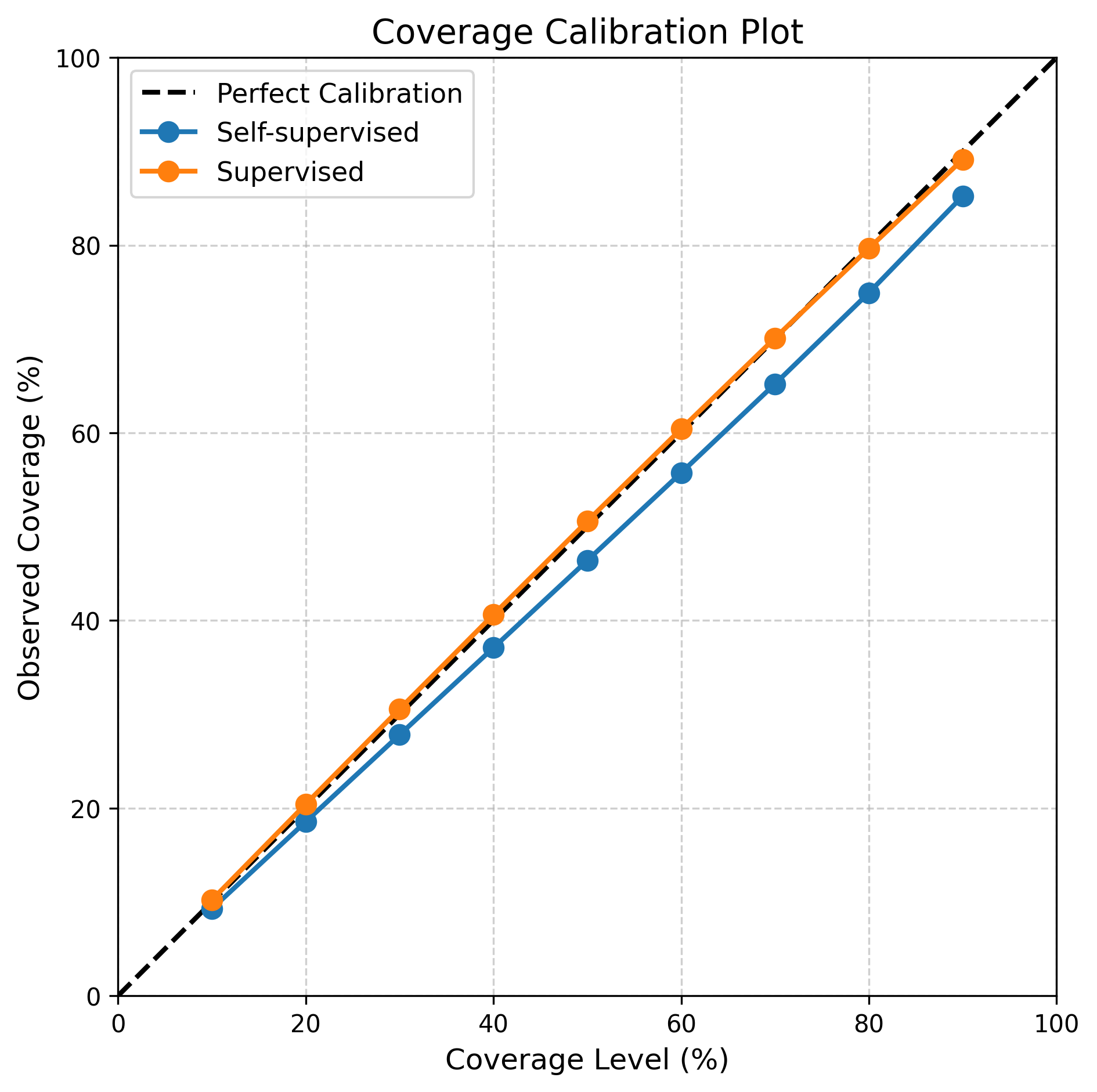
Coverage under a Gaussian probabilistic model.

A common way to evaluate uncertainty is via a coverage test, which defines confidence intervals for a series of nominal confidence levels $\alpha$, and compares the empirical coverage rates with the predicted coverage $\alpha$. The definition of the confidence interval relies on assuming a Gaussian probabilistic model for the posterior distribution, i.e. $u|v\sim\mathcal{N}(\hat{\mu}(v),\Sigma(v)).$ The empirical coverage is computed as the proportion of pixels in the test set for which the ground-truth value falls inside the predicted interval. We plot the coverage test results in Figure 1 (right). We also report the sharpness of the intervals, which is the average length of the $90\%$ confidence intervals, see Table 1. We can see in Table 1 that the supervised model achieves higher PSNR (0.2dB) on the reconstructed HR image. This is consistent with the results obtained in [Nguyen et al., 2022]. In terms of variance RMSE both models are comparable. The sharpness and the coverage plot seem to suggest that the self-supervised variance slightly underestimates the true posterior variance.

5.2 Qualitative evaluation

The uncertainty estimates map in Figure 1 (center) shows a checkerboard effect with a period of two, which inspires to investigate the estimates at 4 different subgrids (corresponding to the four downsampling patterns indicated by the colors in the super-resolved image of Figure 2).

We compare the quality of the uncertainty estimates for these four subgrids. We show the resulting metrics in Table 2. To summarize the calibration curve, we report the Calibration Error (CE) [Kuleshov et al., 2018, Chung et al., 2021] which is computed as $\text{CE}=\frac{1}{m}\sum_{j=1}^{m}|p_{j}-\hat{p}_{j}|$, for each pair of nominal and actual confidence level $p_{j},\hat{p}_{j}$. Coverage plots for the 4 subsets of pixels (see supplementary) show no signs of deviations from the average coverage curve. We see that pixels from the top-left have the smallest RMSE, meaning they match the actual squared prediction error the best. In addition, the estimated ${\hat{\nu}(v)}$ (predicted squared error) is also the smallest among the four positions.

The reason for this comes from the fact that during inference, the reference frame is not removed from the input (as it was done during training). This additional datum provides valuable information about the even pixels of the HR frame, as it is a direct (noisy) observation of those pixels, which creates a reduction in the MSE for those pixels. Interestingly, the variance computed by the network captured this effect even with the self-supervised training.

6 Conclusion

We proposed a self-supervised version of the Gaussian NLL loss for estimation of the aleatoric uncertainty in image restoration problems where the available observations are degraded with a linear degradation operator and contaminated by noise. We study the minimizers of the associated risk, and derive optimality conditions for general linear degradations, and for the specific case of super-resolution with a randomized subsampling operator. We justify the validity of the proposed loss by showing that the posterior mean and variance are among the optimal estimators (in the general linear degradation case), and are the unique minimizers for the randomized subsampling operator, thus showing the equivalence with the supervised Gaussian NLL loss. Finally, we apply this loss to the satellite image super-resolution task on a synthetic satellite image dataset simulated based on L1B [Nguyen et al., 2022], demonstrating obtaining a performance comparable with supervised training.

Future work should explore the application of the proposed loss to other inverse problems. The challenge here is that in the general linear case the posterior mean and variance are not the unique minimizers.

Acknowledgments. Project PID2024-162897NA-I00 funded by MICIU/AEI/10.13039/501100011033/ FEDER, UE. This work was performed using HPC resources from GENCI-IDRIS (grants 2023-AD011011801R3, 2023-AD011012453R2, 2023-AD011012458R2) and from the “Mésocentre” computing center of CentraleSupélec and ENS Paris-Saclay supported by CNRS and Région Île-de-France (http://mesocentre.centralesupelec.fr/). Centre Borelli is also with Université Paris Cité, SSA and INSERM.

Appendix A Mathematical derivations

A.1 Derivative of NLL loss with respect to ${\hat{\Sigma}(v)}$

Proving Lemma 4.1 requires computing the derivative of “per-input risk” $\mathcal{R}_{v}$ eq. (6) w.r.t. ${\hat{\Sigma}(v)}$:

$$\frac{\partial\mathcal{R}_{v}}{\partial{\hat{\Sigma}(v)}}=\mathbb{E}_{\tau,z\mid v}\left[\frac{\partial\mathcal{L}_{\mathrm{NLL}}}{\partial{\hat{\Sigma}(v)}}\right]$$ (16)

Recall that ${\hat{M}}=(A_{\tau}{\hat{\Sigma}(v)}A_{\tau}^{T}+{\hat{R}_{\tau}(v)})^{-1}$, and we denote $\mathcal{L}_{\mathrm{NLL}}$ as $\mathcal{L}$ for simplicity. We can express the differential [Minka, 2000] of $\mathcal{L}$ using the chain rule as:

$$d\mathcal{L}=\mathrm{Tr}\left(\frac{\partial\mathcal{L}}{\partial{\hat{M}}}^{T}d{\hat{M}}\right)$$

$$\frac{\partial\mathcal{L}}{\partial{\hat{M}}}=(z-A_{\tau}\hat{u}(v))(z-A_{\tau}\hat{u}(v))^{T}-{\hat{M}}^{-1}$$

$$d{\hat{M}}=-{\hat{M}}A_{\tau}d\hat{\Sigma}A_{\tau}^{T}{\hat{M}}$$

The above equations lead to

$$d\mathcal{L} =\mathrm{Tr}\left(-\frac{\partial\mathcal{L}}{\partial{\hat{M}}}^{T}{\hat{M}}A_{\tau}d\hat{\Sigma}A_{\tau}^{T}{\hat{M}}\right)$$

$$=\mathrm{Tr}\left(-A_{\tau}^{T}{\hat{M}}\frac{\partial\mathcal{L}}{\partial{\hat{M}}}^{T}{\hat{M}}A_{\tau}d\hat{\Sigma}\right)$$ (17)

Thus,

$$\frac{\partial\mathcal{L}}{\partial\hat{\Sigma}}=\Big(-A_{\tau}^{T}{\hat{M}}\frac{\partial\mathcal{L}}{\partial{\hat{M}}}^{T}{\hat{M}}A_{\tau}\Bigr)^{T}=-A_{\tau}^{T}{\hat{M}}\frac{\partial\mathcal{L}}{\partial{\hat{M}}}{\hat{M}}A_{\tau}$$ (18)

Expanding the term $\frac{\partial\mathcal{L}}{\partial{\hat{M}}}$, we have

$$\frac{\partial\mathcal{L}}{\partial\hat{\Sigma}}=A_{\tau}^{T}{\hat{M}}A_{\tau}-A_{\tau}^{T}{\hat{M}}(z-A_{\tau}\hat{u}(v))(z-A_{\tau}\hat{u}(v))^{T}{\hat{M}}A_{\tau}.$$

A.2 Derivative of NLL loss with respect to ${\hat{\nu}(v)}$

Denote ${\hat{M}}=(A_{\tau}\text{diag}({\hat{\nu}(v)})A_{\tau}^{T})^{-1}$. We consider the differential expression (17) under the diagonal parameterization ${\hat{\Sigma}(v)}=\text{diag}({\hat{\nu}(v)})$. The following holds for the diagonal operator:

$$d\hat{\Sigma}=\text{diag}(d{\hat{\nu}(v)}),$$

which leads to

$$d\mathcal{L} =\mathrm{Tr}\left(\frac{\partial\mathcal{L}}{\partial\hat{\Sigma}}^{T}\;d\hat{\Sigma}\right)=\mathrm{Tr}\left(\frac{\partial\mathcal{L}}{\partial\hat{\Sigma}}^{T}\;\text{diag}(d{\hat{\nu}(v)})\right)$$

$$=\text{diag}\left(\frac{\partial\mathcal{L}}{\partial\hat{\Sigma}}\right)^{T}\;d{\hat{\nu}(v)}.$$ (19)

In this last equation the diag operator is applied to a matrix and thus it acts by extracting its diagional as a column vector. We conclude that

$$\frac{\partial\mathcal{L}}{\partial{\hat{\nu}(v)}}=\text{diag}\left(\frac{\partial\mathcal{L}}{\partial\hat{\Sigma}}\right)=\text{diag}(A_{\tau}^{T}({\hat{M}}-{\hat{M}}{M}^{-1}{\hat{M}})A_{\tau})$$ (20)

References

- Aggarwal et al. [2022] Hemant Kumar Aggarwal, Aniket Pramanik, Maneesh John, and Mathews Jacob. Ensure: A general approach for unsupervised training of deep image reconstruction algorithms. IEEE transactions on medical imaging, 42(4):1133–1144, 2022.
- Aiyetigbo et al. [2024] Mary Aiyetigbo, Alexander Korte, Ethan Anderson, Reda Chalhoub, Peter Kalivas, Feng Luo, and Nianyi Li. Unsupervised microscopy video denoising. In Proceedings of the IEEE/CVF Conference on Computer Vision and Pattern Recognition, pages 6874–6883, 2024.
- Altekrüger and Hertrich [2023] Fabian Altekrüger and Johannes Hertrich. Wppnets and wppflows: The power of wasserstein patch priors for superresolution. SIAM Journal on Imaging Sciences, 16(3):1033–1067, 2023.
- Angelopoulos et al. [2022] Anastasios N Angelopoulos, Amit Pal Kohli, Stephen Bates, Michael Jordan, Jitendra Malik, Thayer Alshaabi, Srigokul Upadhyayula, and Yaniv Romano. Image-to-image regression with distribution-free uncertainty quantification and applications in imaging. In International Conference on Machine Learning, pages 717–730. PMLR, 2022.
- Batson and Royer [2019] Joshua Batson and Loic Royer. Noise2self: Blind denoising by self-supervision. In International conference on machine learning, pages 524–533. PMLR, 2019.
- Bhat et al. [2023] Goutam Bhat, Michaël Gharbi, Jiawen Chen, Luc Van Gool, and Zhihao Xia. Self-supervised burst super-resolution. In Proceedings of the IEEE/CVF international conference on computer vision, pages 10605–10614, 2023.
- Bickford Smith et al. [2025] Freddie Bickford Smith, Jannik Kossen, Eleanor Trollope, Mark Van Der Wilk, Adam Foster, and Tom Rainforth. Rethinking aleatoric and epistemic uncertainty. In Proceedings of the 42nd International Conference on Machine Learning, volume 267 of Proceedings of Machine Learning Research, pages 4345–4359. PMLR, 13–19 Jul 2025. URL https://proceedings.mlr.press/v267/bickford-smith25a.html.
- Bishop [1994] Christopher M Bishop. Mixture density networks. 1994.
- Blundell et al. [2015] Charles Blundell, Julien Cornebise, Koray Kavukcuoglu, and Daan Wierstra. Weight uncertainty in neural network. In International conference on machine learning, pages 1613–1622. PMLR, 2015.
- Braverman et al. [2021] Amy Braverman, Jonathan Hobbs, Joaquim Teixeira, and Michael Gunson. Post hoc uncertainty quantification for remote sensing observing systems. SIAM/ASA Journal on Uncertainty Quantification, 9(3):1064–1093, 2021.
- Chen et al. [2021] Dongdong Chen, Julián Tachella, and Mike E Davies. Equivariant imaging: Learning beyond the range space. In IEEE/CVF International Conference on Computer Vision (ICCV), 2021.
- Chung et al. [2023] Hyungjin Chung, Jeongsol Kim, Michael Thompson Mccann, Marc Louis Klasky, and Jong Chul Ye. Diffusion posterior sampling for general noisy inverse problems. In The Eleventh International Conference on Learning Representations, 2023. URL https://openreview.net/forum?id=OnD9zGAGT0k.
- Chung et al. [2021] Youngseog Chung, Ian Char, Han Guo, Jeff Schneider, and Willie Neiswanger. Uncertainty toolbox: an open-source library for assessing, visualizing, and improving uncertainty quantification. arXiv preprint arXiv:2109.10254, 2021.
- Daras et al. [2023] Giannis Daras, Kulin Shah, Yuval Dagan, Aravind Gollakota, Alex Dimakis, and Adam Klivans. Ambient diffusion: Learning clean distributions from corrupted data. Advances in Neural Information Processing Systems, 36:288–313, 2023.
- Dewil et al. [2021] Valéry Dewil, Jérémy Anger, Axel Davy, Thibaud Ehret, Gabriele Facciolo, and Pablo Arias. Self-supervised training for blind multi-frame video denoising. In Proceedings of the IEEE/CVF winter conference on applications of computer vision, pages 2724–2734, 2021.
- Dorta et al. [2018] Garoe Dorta, Sara Vicente, Lourdes Agapito, Neill DF Campbell, and Ivor Simpson. Structured uncertainty prediction networks. In Proceedings of the IEEE conference on computer vision and pattern recognition, pages 5477–5485, 2018.
- Ebel et al. [2023] Patrick Ebel, Vivien Sainte Fare Garnot, Michael Schmitt, Jan Dirk Wegner, and Xiao Xiang Zhu. Uncrtaints: Uncertainty quantification for cloud removal in optical satellite time series. In Proceedings of the IEEE/CVF Conference on Computer Vision and Pattern Recognition, pages 2086–2096, 2023.
- Ehret et al. [2019a] Thibaud Ehret, Axel Davy, Pablo Arias, and Gabriele Facciolo. Joint demosaicking and denoising by fine-tuning of bursts of raw images. In Proceedings of the ieee/cvf international conference on computer vision, pages 8868–8877, 2019a.
- Ehret et al. [2019b] Thibaud Ehret, Axel Davy, Jean-Michel Morel, Gabriele Facciolo, and Pablo Arias. Model-blind video denoising via frame-to-frame training. In Proceedings of the IEEE/CVF conference on computer vision and pattern recognition, pages 11369–11378, 2019b.
- Gal and Ghahramani [2015] Yarin Gal and Zoubin Ghahramani. Bayesian convolutional neural networks with bernoulli approximate variational inference. arXiv preprint arXiv:1506.02158, 2015.
- Gal and Ghahramani [2016] Yarin Gal and Zoubin Ghahramani. Dropout as a bayesian approximation: Representing model uncertainty in deep learning. In international conference on machine learning, pages 1050–1059. PMLR, 2016.
- Gawlikowski et al. [2023] Jakob Gawlikowski, Cedrique Rovile Njieutcheu Tassi, Mohsin Ali, Jongseok Lee, Matthias Humt, Jianxiang Feng, Anna Kruspe, Rudolph Triebel, Peter Jung, Ribana Roscher, et al. A survey of uncertainty in deep neural networks. Artificial Intelligence Review, 56(Suppl 1):1513–1589, 2023.
- Gruber et al. [2025] Cornelia Gruber, Patrick Oliver Schenk, Malte Schierholz, Frauke Kreuter, and Göran Kauermann. Sources of uncertainty in supervised machine learning–a statisticians’ view. arXiv preprint ArXiv:2305.16703, 2025.
- Haas and Rabus [2021] Jarrod Haas and Bernhard Rabus. Uncertainty estimation for deep learning-based segmentation of roads in synthetic aperture radar imagery. Remote Sensing, 13(8):1472, 2021.
- Hendriksen et al. [2020] Allard Adriaan Hendriksen, Daniël Maria Pelt, and K Joost Batenburg. Noise2inverse: Self-supervised deep convolutional denoising for tomography. IEEE Transactions on Computational Imaging, 6:1320–1335, 2020.
- Hüllermeier and Waegeman [2021] Eyke Hüllermeier and Willem Waegeman. Aleatoric and epistemic uncertainty in machine learning: An introduction to concepts and methods. Machine learning, 110(3):457–506, 2021.
- Kawar et al. [2022] Bahjat Kawar, Michael Elad, Stefano Ermon, and Jiaming Song. Denoising diffusion restoration models. Advances in neural information processing systems, 35:23593–23606, 2022.
- Kendall and Gal [2017] Alex Kendall and Yarin Gal. What uncertainties do we need in bayesian deep learning for computer vision? Advances in neural information processing systems, 30, 2017.
- Kim and Ye [2021] Kwanyoung Kim and Jong Chul Ye. Noise2score: tweedie’s approach to self-supervised image denoising without clean images. Advances in Neural Information Processing Systems, 34:864–874, 2021.
- Kirchhof et al. [2025] Michael Kirchhof, Gjergji Kasneci, and Enkelejda Kasneci. Reexamining the aleatoric and epistemic uncertainty dichotomy. In The Fourth Blogpost Track at ICLR 2025, 2025.
- Krull et al. [2019] Alexander Krull, Tim-Oliver Buchholz, and Florian Jug. Noise2void-learning denoising from single noisy images. In Proceedings of the IEEE/CVF conference on computer vision and pattern recognition, pages 2129–2137, 2019.
- Krull et al. [2020] Alexander Krull, Tomáš Vičar, Mangal Prakash, Manan Lalit, and Florian Jug. Probabilistic noise2void: Unsupervised content-aware denoising. Frontiers in Computer Science, 2:5, 2020.
- Kuleshov et al. [2018] Volodymyr Kuleshov, Nathan Fenner, and Stefano Ermon. Accurate uncertainties for deep learning using calibrated regression. In International conference on machine learning, pages 2796–2804. PMLR, 2018.
- Lahlou et al. [2023] Salem Lahlou, Moksh Jain, Hadi Nekoei, Victor I Butoi, Paul Bertin, Jarrid Rector-Brooks, Maksym Korablyov, and Yoshua Bengio. DEUP: Direct epistemic uncertainty prediction. Transactions on Machine Learning Research, 2023. ISSN 2835-8856. URL https://openreview.net/forum?id=eGLdVRvvfQ. Expert Certification.
- Laine et al. [2019] Samuli Laine, Tero Karras, Jaakko Lehtinen, and Timo Aila. High-quality self-supervised deep image denoising. Advances in neural information processing systems, 32, 2019.
- Lakshminarayanan et al. [2017] Balaji Lakshminarayanan, Alexander Pritzel, and Charles Blundell. Simple and scalable predictive uncertainty estimation using deep ensembles. Advances in neural information processing systems, 30, 2017.
- Lehtinen et al. [2018] Jaakko Lehtinen, Jacob Munkberg, Jon Hasselgren, Samuli Laine, Tero Karras, Miika Aittala, and Timo Aila. Noise2noise: Learning image restoration without clean data. arXiv preprint arXiv:1803.04189, 2018.
- Metzler et al. [2018] Christopher A Metzler, Ali Mousavi, Reinhard Heckel, and Richard G Baraniuk. Unsupervised learning with stein’s unbiased risk estimator. arXiv preprint arXiv:1805.10531, 2018.
- Millard and Chiew [2023] Charles Millard and Mark Chiew. A theoretical framework for self-supervised mr image reconstruction using sub-sampling via variable density noisier2noise. IEEE transactions on computational imaging, 9:707–720, 2023.
- Minka [2000] Thomas P Minka. Old and new matrix algebra useful for statistics, December 2000. URL https://tminka.github.io/papers/matrix/.
- Miranda et al. [2025] Miro Miranda, Francisco Mena, and Andreas Dengel. An analysis of temporal dropout in earth observation time series for regression tasks. In International Symposium on Intelligent Data Analysis, pages 389–402. Springer, 2025.
- Moran et al. [2020] Nick Moran, Dan Schmidt, Yu Zhong, and Patrick Coady. Noisier2noise: Learning to denoise from unpaired noisy data. In Proceedings of the IEEE/CVF conference on computer vision and pattern recognition, pages 12064–12072, 2020.
- Nguyen et al. [2021] Ngoc Long Nguyen, Jérémy Anger, Axel Davy, Pablo Arias, and Gabriele Facciolo. Self-supervised multi-image super-resolution for push-frame satellite images. In Proceedings of the IEEE/CVF Conference on Computer Vision and Pattern Recognition, pages 1121–1131, 2021.
- Nguyen et al. [2022] Ngoc Long Nguyen, Jérémy Anger, Axel Davy, Pablo Arias, and Gabriele Facciolo. Self-supervised super-resolution for multi-exposure push-frame satellites. In Proceedings of the IEEE/CVF Conference on Computer Vision and Pattern Recognition, pages 1858–1868, 2022.
- Nix and Weigend [1994] David A Nix and Andreas S Weigend. Estimating the mean and variance of the target probability distribution. In Proceedings of 1994 ieee international conference on neural networks (ICNN’94), volume 1, pages 55–60. IEEE, 1994.
- Pang et al. [2021] Tongyao Pang, Huan Zheng, Yuhui Quan, and Hui Ji. Recorrupted-to-recorrupted: Unsupervised deep learning for image denoising. In Proceedings of the IEEE/CVF conference on computer vision and pattern recognition, pages 2043–2052, 2021.
- Soltanayev and Chun [2018] Shakarim Soltanayev and Se Young Chun. Training deep learning based denoisers without ground truth data. Advances in neural information processing systems, 31, 2018.
- Tachella and Davies [2026] Julián Tachella and Mike Davies. Self-supervised learning from noisy and incomplete data. arXiv preprint arXiv:2601.03244, 2026.
- Tachella and Pereyra [2024] Julián Tachella and Marcelo Pereyra. Equivariant bootstrapping for uncertainty quantification in imaging inverse problems. In International Conference on Artificial Intelligence and Statistics, pages 4141–4149. PMLR, 2024.
- Tachella et al. [2024] Julián Tachella, Mike Davies, and Laurent Jacques. Unsure: self-supervised learning with unknown noise level and stein’s unbiased risk estimate. arXiv preprint arXiv:2409.01985, 2024.
- Valdenegro-Toro and Mori [2022] Matias Valdenegro-Toro and Daniel Saromo Mori. A deeper look into aleatoric and epistemic uncertainty disentanglement. In 2022 IEEE/CVF Conference on Computer Vision and Pattern Recognition Workshops (CVPRW), pages 1508–1516. IEEE, 2022.
- Valsesia and Magli [2021] Diego Valsesia and Enrico Magli. Permutation invariance and uncertainty in multitemporal image super-resolution. IEEE Transactions on Geoscience and Remote Sensing, 60:1–12, 2021.