Enhancing the Accuracy of Regional Input–Output Table Estimation: A Deep Learning Approach

Abstract

Non-survey methods have been developed and applied for estimating regional input–output tables. However, there is an ongoing debate about the assumptions necessary for these methods and their accuracy.

To address these issues, this study presents a deep learning method for estimating regional input–output tables. First, the quantitative economic data for regions is augmented by linear combinations. Then, deep learning is performed on each item in the input–output table, treating these items as target variables. Finally, regional input–output tables are estimated through matrix balancing to the predicted values from the trained model.

The estimation accuracy of this method is verified using the 2015 input–output table for Japan as a benchmark. Compared to matrix balancing under the ideal assumption of known row and column sums, our method generally demonstrates higher estimation accuracy. Thus, this method is anticipated to provide a foundation for deriving more precise estimates of regional input–output tables.

Keywords Deep learning, regional input–output table, machine learning, data augmentation

1 Introduction

In the context of a macroeconomic quantitative analysis of regional economies, input–output tables represent a fundamental dataset. The creation of input–output tables requires substantial data sources. Regions with limited data sources face considerable challenges in creating these tables. Therefore, much research has focused on developing and improving estimation methods for regional input–output tables.

An input–output table records the flow of products within a target region from two perspectives: producers (input) and consumers (demand). In general, input–output tables are compiled at the national level. Those compiled for domestic regions are referred to as regional input–output tables.

Regional input–output tables are used in various analyses focusing on regional economies. Recently, these tables have frequently been utilized to analyze the effects of environmental policies and disasters. Okuyama [2007] reviewed past studies that analyzed the impact of disasters on regional economies. Some of these studies used regional input–output tables. Koks et al. [2016] evaluated the impact of disasters on regions using various methods based on regional input–output tables, and compared these approaches. Kjaer et al. [2015] calculated the environmental footprint using Denmark’s environmental input–output table.

However, regional input–output tables are rarely compiled and published for small domestic regions. In Japan, for example, the national input–output table is compiled based on primary statistics. Prefectural input–output tables are estimated by combining available partial primary data with data from original surveys. On the other hand, at the municipal level, the availability of primary statistics is even more limited. Consequently, very few municipalities publish their own tables.

In light of this, numerous methods have been developed for estimating regional input–output tables. Particular focus has been placed on a series of methods known as non-survey methods. They estimate input–output tables from published statistics without conducting original surveys in the target region.

Most non-survey methods are designed to estimate input coefficients. An input coefficient is defined as the ratio of intermediate input to the gross output of an input industry. Input coefficients play a crucial role in obtaining the entire input–output table and in calculating economic effects.

The primary non-survey methods employed are the location quotient (LQ) method and the RAS method. These methods require less data and therefore facilitate the estimation of input coefficients, even in small regions where primary statistics are limited.

The ratio of the industry’s share of economic activity in the target economy to its share in a reference economy is denoted as the location quotient [Isserman, 1977]. The LQ method estimates input coefficients for a target region based on the input coefficients of a reference region and the location quotient. Derivatives include CILQ, RLQ, and FLQ [Flegg and Tohmo, 2016]. Moreover, new derivatives have recently been developed, such as FLQ+ and 2DLQ[Pereira-López et al., 2020, Flegg et al., 2021]. Studies such as Bonfiglio and Francesco [2008], Flegg and Tohmo [2012], and Lamonica and Chelli [2018] have verified the accuracy of these derivatives.

The RAS method is regarded as the technique initially introduced in Stone’s research[Bacharach, 1970]. It estimates the input coefficient matrix for a target region by adjusting the initial matrix using the intermediate demands, intermediate inputs, and gross outputs by industry in that region. Hewings [1977] demonstrated that the RAS method can estimate input coefficients for the target region with a high degree of precision. Similar to the LQ method, numerous derivatives and improvements have been developed for the RAS method [Junius and Oosterhaven, 2003, Lenzen et al., 2007, Lemelin, 2009, Lenzen et al., 2014, Temursho et al., 2021]. Furthermore, studies such as Hiramatsu et al. [2016] and Holỳ and Šafr [2023] have sought to improve the RAS method focusing on regional input coefficients.

However, these major non-survey methods require strong assumptions about economic activity, and their validity has been the subject of prolonged debate[Round, 1983]. According to Riddington et al. [2006], the LQ method requires that productivity and consumption per employee must be identical across all regions and that there must be no cross-hauling of products within the same industry. For the RAS method, Miller and Blair [2022] as noted, differences in production technology between the referenced and target regions must be decomposed into substitution and fabrication effects.

For these non-survey methods, as less data is required, the information is also selective. Consequently, the accuracy may be lower than when using more information.

Furthermore, both the LQ and RAS methods necessitate additional data. In the LQ method, the referenced region and economic activity must be selected when calculating the location quotient. The RAS method requires selecting the initial input coefficient matrix and specifying intermediate demands, intermediate inputs, and gross outputs by industry in the target region. These data selection and specification influence the estimation accuracy. For example, Fukui [2025] demonstrated that the estimation accuracy of input coefficients varies depending on the reference region in FLQ and the initial value setting of the input coefficient matrix in RAS.

In recent years, deep learning has been utilized in many fields. A neural network is a function constituted by aligning simple-shaped functions, known as activation functions, and connecting them in layers. Moreover, a neural network with a large number of layers and structures is called a deep neural network. Due to its structure, a deep neural network can precisely capture nonlinear relationships between variables, making it particularly useful for predicting target variables with high accuracy. Training deep neural networks with large datasets is referred to as deep learning. Deep learning serves as the foundational framework for current generative artificial intelligence (AI). It has also frequently been utilized to predict and evaluate asset prices[Ding and Qin, 2020, Srivinay et al., 2022, Chen et al., 2023].

Some studies have sought to incorporate neural networks into the estimation of input coefficients. Papadas and Hutchinson [2002] predicted input coefficients of the United Kingdom using a neural network. Pakizeh and Kashani [2022] estimated input coefficients of nine regions within Japan using machine learning methods, including neural networks. Both studies attempted to ensure sufficient data size by applying a single neural network model to all input coefficients. Nevertheless, it can be inferred that deep neural networks were not applied due to the insufficient size of the data. Training deep neural networks with small data may result in overfitting, which reduces prediction accuracy. In such cases, it is imperative to design the neural network layers to be relatively shallow. Consequently, it appears that the above studies could not achieve a level of prediction accuracy that clearly surpasses that of conventional methods.

Fukui [2025] developed a method for estimating input coefficients with deep learning. This method addressed overfitting through a data augmentation technique called mixup, as described in Zhang et al. [2018]. Compared to conventional methods, the method proposed by Fukui [2025] had the advantage of not necessitating assumptions about economic activity. The method achieved higher precision than conventional methods for estimating input coefficients in the input–output table for Japan. Moreover, as no additional estimation or selection of other data was required, the accuracy of the method was stable.

While a number of methods have been developed to estimate input coefficients (i.e., the intermediate inputs section of an input–output table), few studies have presented standardized methods to estimate other sections, such as final demand, gross value added, and gross output. Simple estimation methods for these sections involve using the ratio of macroeconomic variables between the target and referenced regions. For instance, when estimating gross outputs by industry in a region, one might calculate the ratio of workers in each industry in the region compared to the country. Then, these ratios are multiplied by the gross outputs by industry in the country to obtain the estimates[Kronenberg, 2009]. While this method is straightforward, it may not accurately reflect the region’s or industry’s actual conditions because it disregards information beyond the calculated ratios. Alternatively, there are methods that estimate the items in the sections of final demand, gross value added, and gross output based on data available for the target region[Hosoe, 2014]. These methods can better reflect regional characteristics than the simpler approach. However, the feasibility of these methods depends not only on data availability but also on the researcher’s knowledge and experience.

Given the current state of regional input–output table estimation, this study proposes a novel, deep learning-based method. This method extends the approach in Fukui [2025] to encompass items beyond input coefficients, including final demand, gross value added, and gross output. The generation process for each item in these sections is approximated by a deep neural network that takes various regional economic data as inputs. We expect that this approach will yield highly accurate and stable estimates for items in the input–output table.

Section 2 explains the estimation method for regional input–output tables using a deep learning. Section 3 estimates the 2015 input–output table for Japan and verifies the results. Section 4 discusses the properties and limitations of the proposed method.

2 Data and method

This section presents the estimation method for the 2015 input–output tables, which cover Japan as a whole and the individual cities. The data used to train the model were derived from the 45 prefectures and four cities of Japan, as shown in Table 1.

Table 1: Regions included in the training data

Prefectures
Hokkaido, Aomori, Iwate, Miyagi, Akita,
Yamagata, Fukushima, Ibaraki, Tochigi, Gunma,
Saitama, Chiba, Kanagawa, Niigata, Toyama,
Ishikawa, Fukui, Yamanashi, Nagano, Gifu,
Shizuoka, Aichi, Mie, Shiga, Kyoto,
Osaka, Hyogo, Nara, Wakayama, Tottori,
Shimane, Okayama, Hiroshima, Yamaguchi, Tokushima,
Kagawa, Ehime, Kochi, Fukuoka, Saga,
Nagasaki, Kumamoto, Oita, Miyazaki, Kagoshima
Cities
Saitama (Saitama Pref.), Yokohama (Kanagawa Pref.),
Kawasaki (Kanagawa Pref.), Fukuoka (Fukuoka Pref.)

Table 2: Industry classification

Order	Industry
1	Agriculture, forestry, and fisheries
2	Mining
3	Manufacturing
4	Construction
5	Electricity, gas, heat supply, water supply,
	and waste disposal business
6	Commerce
7	Finance, insurance, and real estate
8	Transport and postal services
9	Information and communications
10	Public administration
11	Service industries
12	Unclassified

The input–output table employed in this study was of the competitive import type, and the industries were reclassified as shown in Table 2. Final demand and gross value added were classified as in Tables 3 and 4, respectively.

In our method, net exports were the target for estimation. Net exports are defined as the difference between exports and imports. As noted in the appendix of Fukui [2025], in a competitive import type input–output table, the sum of exports from two regions does not equal the exports when those regions are combined into one. The same applies to imports. This property does not satisfy the criteria for the data augmentation in the method, a topic that will be elaborated on later. Thus, exports and imports are not suitable for estimation by our method. Conversely, the criteria holds for net exports, rendering them suitable for our model.

In the estimation of input–output tables for cities, the sum of the net exports and the net outflow to other regions within the country was estimated. Net outflow is defined as the difference between outflow and inflow of the city.

The data used for this study are displayed in Table 5. In Table 5, the subscripts $i$ and $j$ represent the order of the industries in Table 2. The subscripts $g$ and $h$ denote the order of final demand in Table 3 and gross value added in Table 4, respectively. Furthermore, $k$ indicate regions, and $c$ is used to denote industry classifications in the Economic Census. For minor industry classifications, $c=1,\ldots,619$ and for major classifications, $c=1,\ldots,17$.

Table 3: Sub-sectors within the final demand sector

Order	Sector
1	Consumption expenditure outside households
2	Consumption expenditure (private)
3	Consumption expenditure of general government
4	Gross regional fixed capital formation
5	Increase in stocks
6	Net exports (or total of net exports and net outflow)

Table 4: Sub-sectors within the gross value added sector

Order	Sector
1	Consumption expenditure outside households
2	Compensation of employees
3	Operating surplus
4	Depreciation of fixed capital
5	Indirect taxes
6	(less) Current subsidies

Table 5: Data used in this study, grouped by source. The definitions of minor and major classifications follow the Economic Census

Variable	Data	Source
$A_{i,j,k}$	Intermediate input	2015 regional input–
	(12 industries, million yen)	output tables
$D_{i,g,k}$	Final demand (12 industries,	published by
	6 sub-sectors, million yen)	each local government
$V_{i,h,k}$	Gross value added (12 industries,
	6 sub-sectors, million yen)
$Y_{i,k}$	Gross output
	(12 industries, million yen)
$\text{Firm}_{c,k}$	Number of establishments	2014 Economic Census
	(major classification)	for Business Frame
$\text{SFirm}_{c,k}$	Number of establishments
	(minor classification)
$\text{SEmp}_{c,k}$	Number of employees
	(minor classification)
$\text{MUnitAg}_{k}$	Number of agriculture	2015 Census of
	management entities	Agriculture and Forestry
$\text{MUnitFo}_{k}$	Number of forestal
	management entities
$\text{ProductsCr}_{k}$	Production valuea	2015 Statistics of Agri-
	(crop subtotal, 100 million yen)	cultural Income Produced
$\text{ProductsAn}_{k}$	Production valuea	and 2015 Agricultural
	(livestock subtotal, 100 million yen)	Output by Municipality
		(Estimates)
$\text{CFArea}_{c,k}$	Total floor area of buildings started	2015 Building Starts
	(non-residential, major classification, $\text{m}^{2}$)
$\text{VA}_{c,k}$	Value added (major	2015 Statistical Observa-
	classification, million yen)	tions of Prefectures and
$\text{Sales}_{c,k}$	Sales (major classification, million yen)	2015 Statistical Observa-
$\text{Income}_{k}$	Taxable income (thousand yen)	tions of Municipalities
$\text{TP}_{k}$	Number of taxpayer
$\text{PopLF}_{k}$	Population in labor force
$\text{Unemp}_{k}$	Number of unemployed
$\text{Pop15}_{k}$	Population aged 15 and overb

• The Ministry of Agriculture, Forestry and Fisheries has estimated the values of each city based on such as the Census of Agriculture and Forestry.

• The values were calculated by the author based on the source data.

Data augmentation was performed based on the data in Table 5 , which was collected from the regions in Table 1, in order to generate data for model training. Using these data of the regions directly for deep learning could lead to overfitting and a subsequent decline in prediction accuracy due to the small data size. To address this issue of overfitting, Fukui [2025] employed a data augmentation technique known as “mixup”, which was proposed by Zhang et al. [2018]. In applying this technique, Fukui [2025] posited the following assumptions: For each quantitative variable underlying the model variables, the value measured by combining multiple regions equals the sum of the values across those regions, and the value measured by scaling a region equals the scaled value of the region. These assumptions were used to establish the prior knowledge that “for a virtual region obtained by linear interpolation (consisting of the above combination and scaling), the feature vectors should lead to an associated target[Fukui, 2025].” Given this prior knowledge, we generated data for virtual regions through linear combinations of data vectors from multiple regions, thereby increasing the amount of data.

In this study as well, this data augmentation was implemented to mitigate the risk of overfitting. During the augmentation process, two to five regions were randomly selected from those in Table 1. The weights for the linear combination of these regions were generated using random numbers from a Dirichlet distribution with all elements of the parameter vector set to one.

Moreover, this study introduced a method described in Fukui [2025] to address the decline in prediction accuracy caused by the difference in scale between the trained and predicted regions. Since most of the observations were prefectures, the data augmented by the above method notably reflected the scale of prefectures. Consequently, neural network models trained using the generated data showed reduced accuracy for our prediction targets, such as the entire country or municipalities. To address this issue, the quantitative data of the prefectures was converted into per capita data for the population aged 15 and over in 2015, and the data was augmented. This augmented quantitative data was then multiplied by such population of each target area to yield training data reflecting the scale of the prediction targets.

To obtain the training data for Japan as a whole, the augmented data was multiplied by the population aged 15 and over for Japan in 2015. To augment data on cities, we first generated a set of uniform random numbers within the range of the minimum and maximum values of the population aged 15 and over across all cities in Japan in 2015. Next, we multiplied these random numbers by each observation in the augmented data to obtain the city training data.

The values of the explanatory and target variables were calculated from the augmented data. As shown in Table 6, the explanatory variables were derived from the quantitative variables presented in Table 5. The indices of the explanatory variables are identical to those in Table 5.

Table 6: Explanatory variables

Name	Definition
Number of establishments (minor classification)	$\text{SFirm}_{c,k}$
Proportion of establishments by industry	$\text{SFirm}_{c,k}/\sum_{c}\text{SFirm}_{c,k}$
(minor classification)
Number of employees (minor classification)	$\text{SEmp}_{c,k}$
Proportion of employees by industry	$\text{SEmp}_{c,k}/\sum_{c}\text{SEmp}_{c,k}$
(minor classification)
Number of agriculture management entities	$\text{MUnitAg}_{k}$
Number of forestal management entities	$\text{MUnitFo}_{k}$
Production value (crop subtotal)	$\text{ProductsCr}_{k}$
Production value (livestock subtotal)	$\text{ProductsAn}_{k}$
Total floor area of buildings started	$\text{CFArea}_{c,k}$
(major classification)
Proportion of total floor area of building	$\text{CFArea}_{c,k}/\sum_{c}\text{CFArea}_{c,k}$
started by industry (major classification)
Value added (major classification)	$\text{VA}_{c,k}$
Value added per establishment	$\text{VA}_{c,k}/\text{Firm}_{c,k}$
(major classification)
Sales (major classification)	$\text{Sales}_{c,k}$
Sales per establishment (major classification)	$\text{Sales}_{c,k}/\text{Firm}_{c,k}$
Taxable income	$\text{Income}_{k}$
Taxable income per taxpayer	$\text{Income}_{k}/\text{TP}_{k}$
Population in labor force	$\text{PopLF}_{k}$
Labor force participation rate	$\text{PopLF}_{k}/\text{Pop15}_{k}$
Unemployment rate	$\text{Unemp}_{k}/\text{PopLF}_{k}$

In order to eliminate the potential impact of regional economic scale, the ratio to the total of gross outputs for each item in the input–output table was used as the target variable. Given that economic scale positively correlates with each item in the input–output table and with multiple quantitative variables included in the explanatory variables, it can be inferred that a similar correlation exists between the items in the input–output tables and the explanatory variables. When this correlation is pronounced, the trained model reflects of the relationship notably. To mitigate the influence of this correlation, the following variables were used as the target variables:

$$y_{i,k} =Y_{i,k}/\sum_{i}Y_{i,k}\quad\forall k,$$

$$a_{i,j,k} =A_{i,j,k}/\sum_{i}Y_{i,k}\quad\forall i,j,k,$$

$$d_{i,g} =F_{i,g,k}/\sum_{i}Y_{i,k}\quad\forall i,g,k,$$

$$v_{i,h} =V_{i,h,k}/\sum_{i}Y_{i,k}\quad\forall i,h,k.$$

No model was set for the target variables for which all values in the regions of Table 1 were zero, and their predicted values were also set to zero.

Consequently, estimating total of gross outputs is required separately for the method of this study.

Prior to model training, 50,000 samples were generated using the aforementioned data augmentation. Of these, 80% (40,000 samples) were randomly selected as the training data, and the remaining 20% (10,000 samples) served as the test data. We estimated the model parameters using the training data. Subsequently, predictions were made on the test data, and the model was verified by calculating the prediction error.

Figure 1: The neural network model employed in this study

Figure 1 illustrates the model for each item in an input–output table. Prior to the calculation in the model, the explanatory variables in Table 6 were standardized and converted to principal component scores. These scores were processed through a rectified linear unit (ReLU) layer comprising 512 nodes, followed by a stack of ten layers. Each layer in the stack comprised a ReLU layer (512 nodes), a skip connection, and a batch normalization layer. The value calculated from the stack was then used by the output layer to generate the target variable value.

In a batch normalization layer, the inputs are normalized with each training data batch, followed by a linear transformation[Ioffe and Szegedy, 2015]. In a skip connection, the intermediate layer explains the differences between the inputs and outputs[He et al., 2016]. Both batch normalization and skip connections are said to improve the estimation accuracy of model parameters. Furthermore, dropout layers were positioned after the fourth and ninth layers in middle layer to prevent overfitting. A dropout layer is constituted by nodes that discard their inputs with a specified probability[Srivastava et al., 2014].

Different output layers were configured depending on the target variable. Assuming the values of each $y_{i,k}$ and $a_{i,j,k}$ are non-negative, a sigmoid function was established for their output layer. However, when the values of $y_{i,k}$ and $a_{i,j,k}$ were too small, optimization processes were susceptible to failure due to gradient vanishing in the output layer. To circumvent the problem, we adopted a target value transformation similar to that demonstrated in Fukui [2025]. The following transformed variable $y^{*}$ for each of the variables $y_{i,k}$ and $a_{i,j,k}$ was designated as the target variables:

$$y^{*} =\frac{y-y_{l}}{y_{u}-y_{l}}$$ (1)

$$y_{l} =\max(0,\min(y)-0.1*(\max(y)-\min(y)))$$

$$y_{u} =\min(1,\max(y)+0.1*(\max(y)-\min(y))).$$

In this equation, $y$ represents the each variable of the $y_{i,k}$ and $a_{i,j,k}$. Moreover, $\min(y)$ and $\max(y)$ denote the minimum and maximum values of $y$, respectively. On the other hand, given that each of $d_{i,g}$ and $v_{i,h}$ can be both positive and negative, an identity function was implemented as the output layer. The target variable in the output layer was set to the the standardized variable of each $d_{i,g}$ and $v_{i,h}$.

These transformations for the model variables were performed on the training data. The values employed for the transformation (means, standard deviations, minimum and maximum values, principal component loadings, and so on) were used in the prediction phase.

The training was carried out in the following settings: The mean squared error was configured as the loss function. The loss function incorporated an $L_{1}$ regularization term with a parameter of $10^{-5}$. The optimization method employed was stochastic gradient descent with a mini-batch size of 32. Additionally, for parameter updates in the stochastic gradient descent, Nesterov’s accelerated gradient method was applied with a parameter of $0.9$. The learning rate was updated exponentially and periodically according to the method proposed by Smith [2017]. The initial value and lower bound was $10^{-6}$, the upper bound was $0.01$, and the step size between the upper and lower bounds was 10. The updates to the learning rate and parameter values were performed simultaneously. The maximum number of epochs for the training was set to 200, with early stopping. First, 20% of the training data was randomly selected for validation during the model training. Then, the training process was terminated when the error on the validation data (validation error) increased for 10 consecutive epochs. Finally, the parameter values immediately preceding the increase in the validation error were adopted as the training result.

Subsequently, the trained neural network was used to predict each element of the regional input–output table. For the region under prediction, the explanatory variables were standardized, and their principal component scores were calculated. This calculation employed the mean, standard deviation, and principal component loadings recorded for each explanatory variable before training. The principal component scores were fed into the trained neural network. The output of this process was each transformed element of the regional table. As previously mentioned, given that the outputs were also transformed, an inverse transformation was performed using the means, standard deviations, and the values of $y_{l}$ and $y_{u}$ of the target variables used for the transformation prior to training. For each variable $y_{i,k}$ and $a_{i,j,k}$, the predicted value $y$ was obtained by performing the inverse transformation of Eq. (1) to the output $y^{*}$ from the model as follows, using the values of $y_{l}$ and $y_{u}$ of the training data:

$$y=y_{l}+y^{*}(y_{u}-y_{l}).$$

For each $d_{i,g}$ and $v_{i,h}$, the inverse transformation from the model output $y^{*}$ to the predicted value $y$ was as follows:

$$y=\mu_{y}+s_{y}y^{*}.$$

Here, $\mu_{y}$ and $s_{y}$ are the mean and standard deviation of the training data, respectively.

In order to estimate the regional input–output table using our trained model, the outputs from the model must be multiplied by $\sum_{i}Y_{i,k}$.

The gross outputs ($Y_{i,k}$) were predicted for each industry individually. Consequently, the sum of these predicted outputs was not guaranteed to match the actual total of gross outputs. To ensure that, the following processing was applied to each $Y_{i,k}$ predicted by the model. The processed value $Y^{*}_{i,k}$ was then used as the predicted gross output.

$$Y^{*}_{i,k}=\frac{\tilde{Y}_{i,k}}{\sum_{i}\tilde{Y}_{i,k}}\sum_{i}Y_{i,k}$$

where $\tilde{Y}_{i,k}$ is the gross output for industry $i$ from the model for the region $k$.

A matrix balancing procedure was subsequently implemented to ensure that the predicted values satisfied the input–output table constraints. The RAS method, a non-survey technique, is frequently employed for matrix balancing. However, it should be noted that the RAS method is not directly applicable to matrices that contain negative values. To address this issue, Junius and Oosterhaven [2003] proposed the generalized RAS (GRAS) method. The GRAS method is a matrix balancing technique based on cross-entropy maximization. In this study, cross-entropy maximization based on GRAS was performed for matrices containing negative values, subject to the following two conditions. First, the row sums and column sums of the input–output table were equal to the gross outputs by industry. Second, the total of consumption expenditures outside households in the gross value added and final demand sectors were equal to each other.

3 Result

Under the configurations described in the previous section, we estimated the 2015 input–output table for Japan, and the accuracy of our method was verified. The input–output tables for Japan that are available to the public are derived using a survey method, and their high levels of accuracy make them suitable as benchmarks.

The total of gross outputs required in the estimation process used the actual values of the 2015 input–output tables. The model input consisted of the top 60 principal component scores with the highest contribution.

No large difference in prediction error was observed between the training and test data for the trained model. Therefore, each model was considered valid.

Table 7: Prediction errors for 2015 input–output table for Japan

	STPE	MAD	$\text{U}_{2}$	RMSE	MAPE
All	0.0616	619,307.2	0.0543	1,712,645.36	0.4191
Intermediate input	0.0782	286,709.69	0.0831	1,075,781.83	0.1012
Final demand	0.0915	1,038,190.97	0.0838	2,015,753.37	1.6485
(Excluding net	0.0618	809,999.27	0.0675	1,788,321.33	0.5893
export)
(Net export only)	0.5402	2,019,415.26	0.4074	2,789,889.95	6.2033
Gross value added	0.0524	415,501.79	0.0499	856,194.36	0.1307
Gross output	0.0413	3,505,808.89	0.0435	5,451,426.54	0.0621

Table 7 presents various indicators of the prediction error of the input–output table for Japan estimated with the method of this study. These indicators were selected based on Hosoe [2014] and calculated according to the following definitions:

STPE $$=\sum_{i}\left|\tilde{X}_{i}-X_{i}\right|/\sum\left|X\right|_{i}$$

MAD $$=\sum_{i}\left|\tilde{X}_{i}-X_{i}\right|/N_{1}$$

$$\text{U}_{2} =\sqrt{\sum_{i}\left(\tilde{X}_{i}-X_{i}\right)^{2}}/\sqrt{\sum_{i}X^{2}_{i}}$$

RMSE $$=\sqrt{\left[\sum_{i}\left(\tilde{X}_{i}-X_{i}\right)^{2}\right]/N_{1}}$$

MAPE $$=(1/N_{2})\sum_{i}\left|(\tilde{X}_{i}-X_{i})/X_{i}\right|$$

For any indicator, a smaller value indicates a smaller prediction error. In these definitions, $i$ represents index for each item in the input–output table, $X_{i}$ is the actual value for $i$, $\tilde{X}_{i}$ is the corresponding estimated value. $N_{1}$ denotes the number of items where $X_{i}\neq 0\ \text{and}\ \tilde{X}_{i}\neq 0$, and $N_{2}$ is the total number of items whose actual values are neither zero nor empty in the actual input–output table.

(a) Levels of error. Color-coded on a logarithmic scale

(b) Error rates

Figure 2: Prediction errors (millions of yen) and error rates (%) for each item in the input–output table for Japan. Each cell represents an absolute value. Items without published values are left blank

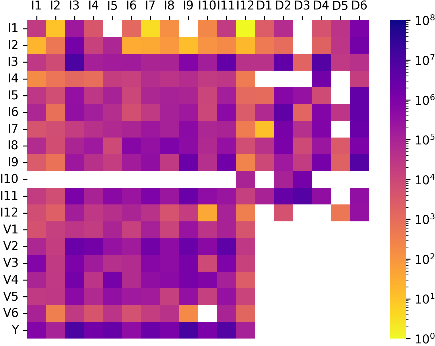
Figures 2(a) and 2(b) are heatmaps representing the levels of error and error rates, respectively, for each item in the input–output table for Japan. These figures follows the structure of the input–output table. The labels “I1”, $\cdots$, “I12” correspond to the order in Table 2, “D1”, $\cdots$, “D6” correspond to the order in Table 3, “V1”, $\cdots$, “V6” correspond to the order in Table 4. Moreover, the label “Y” denotes gross outputs by industry.

Figure 2(a) reveals a positive correlation between the magnitude of error and the gross output of the corresponding industry. Industries with smaller gross output, such as agriculture, forestry, fisheries, and mining, tend to have smaller errors. In Figure 2(b), the error rates are generally high for items of final demand, particularly net exports.

Figure 3: Bar plot of prediction error rates for each item in the input–output table for Japan. Note that the rightmost bar represents the frequency of items with error rates greater than or equal to 100%, while the leftmost bar represents the frequency with error rates less than or equal to 100%

Furthermore, Figure 3 shows a bar plot of the error rates. The figure indicates that the prediction error rates for 159 items fall within the range of [-10%, 10%), which corresponds to approximately 55% of all items (including empty items, for a total of 288).

We compared the accuracy of the proposed method with that of conventional non-survey methods. As Morrison and Smith [1974] stated, the RAS method is usually more accurate than the LQ method when the actual values for row and column totals are available. However, input–output tables generally contain negative values. This makes it inappropriate to use the RAS method directly.

Therefore, as a conventional method, we adopted matrix balancing via cross-entropy maximization utilized also in our method. In this matrix balancing, the actual values of gross outputs by industry of Japan in 2015 were used as the row and column totals. Moreover, the 2011 input–output table for Japan and the 2015 input–output tables for each prefecture were employed as the initial values for the matrix balancing.

Table 8: Comparison of estimation errors in the input–output table for Japan. The values in the second and third rows were derived from the cross-entropy maximization

	STPE	MAD	$\text{U}_{2}$	RMSE	MAPE
Our method	0.0616	619,307.2	0.0543	1,712,645.36	0.4191
Based on 2011 table	0.0609	611,122.95	0.05848	1,849,283.51	0.5673
Based on 2015 tables	0.0921	936,386.96	0.0817	2,590,120.89	0.5996
for each prefecture
(minimum values)

Table 8 shows the estimation errors associated with the conventional methods. Using the 2011 table for Japan as the initial value yielded smaller errors than using the 2015 tables for prefectures. Compared to these errors, our method generally produced even smaller errors, except that the STPE and MAD were slightly larger than the errors of the estimates based on the 2011 table for Japan.

Table 9: Estimation errors of the 2015 input–output table for Japan using cross-entropy maximization with the 2011 table as the initial values. Due to the use of actual values for gross outputs by industry, the errors were zero

	STPE	MAD	$\text{U}_{2}$	RMSE	MAPE
All	0.0609	611,122.95	0.0585	1,849,283.51	0.5673
Intermediate input	0.1019	382,716.03	0.0858	1,123,784.12	0.3589
Final demand	0.1088	1,204,079.56	0.1307	3,146,936.67	1.5716
(Excluding net	0.0871	1,102,510.08	0.1222	3,245,723.25	1.7398
export)
(Net export only)	0.4358	1,630,671.41	0.3932	2,692,744.4	0.8483
Gross value added	0.0862	683,274.31	0.1017	1,744,021.36	0.2852
Gross output	0.0	0.0	0.0	0.0	0.0

Table 9 shows the estimation errors for each sector using the conventional method. This initial value of the method was the 2011 input–output table for Japan. Compared to Table 7, the errors for intermediate inputs, final demand (excluding MAPE), and gross value added were larger than the errors from our method. However, for net exports in the final demand sector, the errors were smaller than those produced by our method.

The overall errors were closer between the two methods compared to the errors by sector. This was due to the presence or absence of estimation of gross outputs by industry. In our method, estimation errors occurred for these gross outputs because they were estimation targets. In contrast, the conventional method used actual measured values for these gross outputs. Consequently, as shown in Table 9, the errors were zero. It is plausible that the discrepancies in the estimation of gross outputs by industry affected the overall error. Excluding them, the STPE and MAD were $0.0743$ and $481,307.12$, respectively, using our method, and $0.0991$ and $640,813.13$, respectively, using the conventional method. Our method yielded smaller values for other indicators as well.

Using the method developed in this study, we estimated input–output tables for each of the three cities in Japan: Sapporo, Gujo, and Okayama. The estimation employed the published gross production values for each city, and the top 100 principal component scores with the highest contribution were selected as the inputs for the model. Subsequently, we compared the input–output tables published by these three cities with the estimates.

The estimates derived from our method differed relatively large from the published values of the three cities for certain items. The sub-tables in Table 10 show the differences between the estimated and published values for the three cities, as measured by STPE, MAD, $\text{U}_{2}$, RMSE, and MAPE. The sub-figures in Figure 4, 5, and 6 display heatmaps of the differences and difference rates for each item in the input–output tables for each city.

Examining the STPE, $\text{U}_{2}$, and MAPE in Table 10, which are independent of the magnitude of the amounts, exhibit that their values for the three cities were generally higher than those for Japan. Particularly for the final demands of Okayama City, the MAPE was notably large. As illustrated in Figure 4, 5, and 6, there were positive correlations between the gross outputs by industry and these levels of differences similar to when the input–output table for Japan was estimated. Moreover, these figures reveal a tendency for high difference rates in inputs for mining in all cities. Sapporo City exhibited high difference rates in inputs associated with agriculture, forestry, and fisheries, as well as manufacturing. Gujo City exhibited high difference rates in inputs related to electricity, gas, and water supply.

Table 10: Differences between estimated and published values of the input–output tables for the three cities

(a) Sapporo City

	STPE	MAD	$\text{U}_{2}$	RMSE	MAPE
All	0.2836	34,865.25	0.2768	103,627.72	2.97
Intermediate input	0.46	14,261.55	0.7341	53,983.27	2.566
Final demand	0.2357	46,044.0	0.2026	82,581.09	1.7841
(Excluding net export)	0.1959	32,761.71	0.1849	67,712.0	2.0149
(Net export only)	0.3264	103,157.85	0.2324	128,175.42	0.792
Gross value added	0.2474	24,919.91	0.1968	47,802.69	4.7716
Gross output	0.2896	257,299.97	0.2889	397,695.21	2.0569

(b) Gujo City

	STPE	MAD	$\text{U}_{2}$	RMSE	MAPE
All	0.2872	789.95	0.2287	1,948.58	2.3382
Intermediate input	0.2491	232.33	0.1478	483.1	0.9138
Final demand	0.3508	1,312.44	0.3697	2,698.03	5.6894
(Excluding net export)	0.2598	917.84	0.3079	2,306.06	4.6207
(Net export only)	0.65	3,009.22	0.6184	3,964.03	10.2846
Gross value added	0.4804	978.94	0.482	2,207.45	2.6
Gross output	0.1486	3,157.61	0.1319	4,365.02	0.7508

(c) Okayama City

	STPE	MAD	$\text{U}_{2}$	RMSE	MAPE
All	0.3447	17,297.46	0.4101	60,707.5	9.7622
Intermediate input	0.4414	6,846.4	0.7077	30,544.7	1.3049
Final demand	0.4368	30,337.7	0.5683	78,142.05	44.7271
(Excluding net export)	0.2184	16,101.99	0.2242	33,512.15	55.9721
(Net export only)	1.6498	84,433.42	2.0824	158,246.71	1.9963
Gross value added	0.2581	10,442.13	0.2143	19,101.08	2.7065
Gross output	0.2915	115,733.1	0.3601	206,160.0	0.5674

(a) Levels of difference. Color-coded on a logarithmic scale

(b) Difference rates

Figure 4: Levels of difference (millions of yen) and difference rates (%) between estimates and published values for each item in the input–output tables for Sapporo City. Each cell represents an absolute value. Items without published values are left blank

(a) Levels of difference. Color-coded on a logarithmic scale

(b) Difference rates

Figure 5: Levels of difference (millions of yen) and difference rates (%) between estimates and published values for each item in the input–output tables for Gujo City. Each cell represents an absolute value. Items without published values are left blank

(a) Levels of difference. Color-coded on a logarithmic scale

(b) Difference rates

Figure 6: Levels of difference (millions of yen) and difference rates (%) between estimates and published values for each item in the input–output tables for Okayama City. Each cell represents an absolute value. Items without published values are left blank

However, it is important to note that the above results do not necessarily represent estimation accuracy. Therefore, it was not possible to reach a definitive conclusion about the validity of the method developed in this study for estimating input–output tables for three cities in Japan. Estimation accuracy is determined by comparing estimates with true values or values close to them. The input–output tables published by these cities, however, were estimated using non-survey or hybrid methods due to the insufficient primary statistics required for their compilation. These methods have larger estimation errors compared to survey method and do not guarantee proximity to true values. Consequently, the estimation accuracy of the input–output tables of these cities could not be determined by comparing the estimates with the published values.

4 Discussion

This study proposed a method for estimating regional input–output tables using deep learning. The properties of this method were verified by estimating input–output tables for regions in Japan.

The proposed method generally achieved higher accuracy in estimating the input–output table for Japan compared to conventional methods. When estimating the 2015 input–output table for Japan, the conventional matrix balancing using the 2011 table and the 2015 gross outputs by industry, both of which were obtained through survey methods, represents an estimation under particularly ideal assumptions. In comparison with the conventional method based on these assumptions, our method generally produced lower errors. This is a noteworthy observation.

The high accuracy of this method is primarily attributable to the implementation of deep learning. This study addressed overfitting in deep learning by generating virtual regions through data augmentation. When the model was trained on the augmented data, the prediction accuracy extrapolated to the input–output table for Japan was satisfactory, indicating that data augmentation effectively mitigated overfitting.

Compared to more precise conventional methods, this study may achieve equivalent accuracy. Hosoe [2014] estimated the 2005 Japan input–output table by balancing the past tables revised with the available data at that time. The results showed that MAPE was approximately 40%, and 53% of the table’s 486 items had an error rate within $[-10\%,10\%)$. In contrast, the method proposed in this study yielded a MAPE of approximately 43% and an error rate within $[-10\%,10\%)$ for approximately 55% of all items. Based solely on these metrics, the prediction accuracy of the two methods can be considered comparable.

The method proposed in this study circumvents the instability associated with selecting reference values, which was necessary in conventional estimation methods. Both cross-entropy maximization and the RAS method require an initial table for calculation. The LQ method requires selecting the target region to derive location quotients. These selections can affect estimation accuracy. As shown in Table 8, the conventional cross-entropy maximization exhibited varying estimation accuracy depending on the initial table selected. In contrast, while our method requires the establishment of explanatory variables, it does not necessitate selecting a small number of reference values as conventional methods do. Therefore, it does not exhibit the accuracy fluctuations observed in conventional methods.

In comparison with cross-entropy maximization and the RAS method, our approach has the additional advantage of requiring fewer specified values in advance. For example, the cross-entropy method requires gross outputs by industry, which serve as the row and column sums during balancing. In contrast, our method merely requires the total of gross outputs. In general, the estimation of the total is less challenging than that of the gross outputs for each industry. For Japanese municipalities, estimating the total of gross outputs is relatively straightforward because various data sources, such as the Economic Census, are available.

Although our method demonstrated higher accuracy than conventional approaches in estimating the input–output table for Japan than conventional approaches, its efficacy in smaller regions, such as cities, remains to be elucidated. In three cities of Japan, relatively large differences were observed between our estimates and the published values for certain items. If these differences are attributable to city-specific characteristics, our model may not fully capture them. Furthermore, the regions used for training were predominantly prefectures. Consequently, the model may not accurately reflect the properties of cities. However, it is important to acknowledge that the published values for these cities are also estimates and may not accurately reflect the true values.

The accuracy of certain items of final demand, particularly net exports, could be improved. One potential improvement would be to introduce explanatory variables that correlate more closely with these items. However, this study could not identify suitable variables for small-area estimation.

The method of this study does not entirely supplant conventional methods. Because our method alone is incapable of satisfying the constraints of input–output tables, the conventional matrix balancing method must be used alongside it. Moreover, our method is limited in its ability to directly estimate exports and imports. Therefore, alternative methods are required to estimate them.

While the proposed method is amenable to improvement and has certain limitations, it can serve as a foundation for obtaining input–output tables in regions where compiling them using primary data is difficult. Such regions are not exclusive to Japan. The compilation of national-level tables may also pose challenges in certain countries. For these regions, our methodology could facilitate the creation of more precise and stable input–output tables compared to conventional methods.

Appendix A An overview of the matrix balancing using cross-entropy maximization

This section provides an overview of the matrix balancing employed in this study.

To ensure that the estimated input–output table satisfies the relevant constraints, matrix balancing was implemented in this study. The method was based on the cross-entropy maximization formulation by Chlebus and Kasapu [2023]. The objective function of the GRAS method, as described in Junius and Oosterhaven [2003] and Lenzen et al. [2007] was incorporated into the formulation, along with additional constraints regarding non-household consumption expenditure.

Let $K$ be the number of industries in an input–output table, $L$ be the number of sub-sectors in gross value added, and $M$ be the number of sub-sectors in final demand. The row and column indices of the input–output table are denoted by $i$ and $j$, respectively. For each item in the table, we denote the value divided by the total of gross outputs as $p_{i,j}\ (1\leq i\leq K+L,1\leq j\leq K+M)$, which is estimated using matrix balancing. An initial input–output table is required for this estimation. For the initial table, we also use the value divided by the total of gross outputs for each item, denoted by $p^{0}_{i,j}\ (1\leq i\leq K+L,1\leq j\leq K+M)$.

The purpose of matrix balancing is to identify the values of $p_{i,j}$ that minimize the following objective function:

$$-\sum_{i=1}^{K+L}\sum_{j=1,p^{0}\geq 0}^{K+M}p_{i,j}\log\frac{p_{i,j}}{e\cdot p^{0}_{i,j}}+\sum_{i=1}^{K+L}\sum_{j=1,p^{0}<0}^{K+M}\log\frac{p_{i,j}}{e\cdot p^{0}_{i,j}}.$$ (2)

Notation $p^{0}\geq 0$ indicates that the sum is comprised exclusively of terms where $p^{0}$ is greater than or equal to zero. Conversely, $p^{0}<0$ denotes that the sum consists only of terms where $p^{0}_{i,j}$ is less than zero. Elements in which $i>K$ and $j>K$ are excluded from the objective function due to their absence.

In the minimization process, certain constraints must be satisfied. In input–output tables, the total input and total demand for an industry are equal to the gross output of that industry. Therefore, the following constraints must be considered:

$$\sum_{j=1}^{K+M}p_{i,j}=y_{i},\quad 1\leq i\leq K$$ (3)

$$\sum_{i=1}^{K+L}p_{i,j}=y_{j},\quad 1\leq j\leq K,$$ (4)

where $y_{i}$ is the gross output of industry $i$ divided by the total of the gross outputs. When $i=j$, it follows that $y_{i}=y_{j}$.

In the input–output tables of Japan, it is customary to include a sub-sector of consumption expenditure outside households in both final demand and gross value added. The totals of consumption expenditure outside households across all industries in final demand and gross value added must be equal each other. Therefore, the following constraint is imperative:

$$\sum_{j=1}^{K}p_{\phi,j}=\sum_{i=1}^{K}p_{i,\phi},$$ (5)

where $\phi\ (\phi>K)$ represents the index of consumption expenditure outside households sector in final demand and gross value added.

From the objective function and constraints enumerated above, the first-order conditions for optimization with Lagrange multipliers specify that the estimates of $p_{i,j}$, obtained through matrix balancing, are as follows:

$$\text{For intermediate input}\ (1\leq i\leq K,1\leq j\leq K)\text{:}$$

$$\qquad p_{i,j}=\begin{cases}p^{0}_{i,j}\exp(\lambda_{i}+\tau_{j}),\quad p^{0}_{i,j}\geq 0\\ p^{0}_{i,j}\exp(-\lambda_{i}-\tau_{j}),\quad p^{0}_{i,j}<0\\ \end{cases}$$ (6)

For final demand without consumption expenditure outside households

$$\ (1\leq i\leq K,K<j\leq K+M,j\neq\phi)\text{:}$$

$$\qquad\quad p_{i,j}=\begin{cases}p^{0}_{i,j}\exp(\lambda_{i}),\quad p^{0}_{i,j}\geq 0\\ p^{0}_{i,j}\exp(-\lambda_{i}),\quad p^{0}_{i,j}<0\\ \end{cases}$$ (7)

For gross value added without consumption expenditure outside

$$\text{households}\ (K<i\leq K+L,i\neq\phi,1\leq j\leq K)\text{:}$$

$$\qquad p_{i,j}=\begin{cases}p^{0}_{i,j}\exp(\tau_{j}),\quad p^{0}_{i,j}\geq 0\\ p^{0}_{i,j}\exp(-\tau_{j}),\quad p^{0}_{i,j}<0\\ \end{cases}$$ (8)

For consumption expenditure outside households in final demand

$$(1\leq i\leq K,j=\phi)\text{:}$$

$$\qquad p_{i,\phi}=\begin{cases}p^{0}_{i,\phi}\exp(\lambda_{i}-\eta),\quad p^{0}_{i,j}\geq 0\\ p^{0}_{i,\phi}\exp(-\lambda_{i}+\eta),\quad p^{0}_{i,j}<0\\ \end{cases}$$ (9)

For consumption expenditure outside households in gross value added

$$(i=\phi,1\leq j\leq K)\text{:}$$

$$\qquad p_{\phi,j}=\begin{cases}p^{0}_{\phi,j}\exp(\tau_{j}+\eta),\quad p^{0}_{i,j}\geq 0\\ p^{0}_{\phi,j}\exp(-\tau_{j}-\eta),\quad p^{0}_{i,j}<0,\\ \end{cases}$$ (10)

where $\lambda_{i}$, $\tau_{j}$, and $\eta$ are the Lagrange multipliers associated with the constraint equations of Eq. (3), (4), and (5), respectively.

The expressions for $\exp(\lambda_{i})$, $\exp(\tau_{j})$, and $\exp(\eta)$ are derived from the above equations, along with Eq. (3), (4), and (5):

$$\left(\sum_{j=1,p^{0}\geq 0}^{K}p^{0}_{i,j}\exp(\lambda_{i})\exp(\tau_{j})+\sum_{j=1,p^{0}<0}^{K}\frac{p^{0}_{i,j}}{\exp(\lambda_{i})\exp(\tau_{j})}\right)$$

$$\quad+p^{0}_{i,\phi}\frac{\exp(\lambda_{i})}{\exp(\eta)}+\left(\sum_{\begin{subarray}{c}j=K+1,j\neq\phi,\\ p^{0}\geq 0\end{subarray}}^{K+M}p^{0}_{i,j}\exp(\lambda_{i})+\sum_{\begin{subarray}{c}j=K+1,j\neq\phi,\\ p^{0}<0\end{subarray}}^{K+M}\frac{p^{0}_{i,j}}{\exp(\lambda_{i})}\right)$$

$$=y_{i},\ (1\leq i\leq K,\ p^{0}_{i,\phi}\geq 0)$$ (11)

$$\left(\sum_{j=1,p^{0}\geq 0}^{K}p^{0}_{i,j}\exp(\lambda_{i})\exp(\tau_{j})+\sum_{j=1,p^{0}<0}^{K}\frac{p^{0}_{i,j}}{\exp(\lambda_{i})\exp(\tau_{j})}\right)$$

$$\quad+p^{0}_{i,\phi}\frac{\exp(\eta)}{\exp(\lambda_{i})}+\left(\sum_{\begin{subarray}{c}j=K+1,j\neq\phi,\\ p^{0}\geq 0\end{subarray}}^{K+M}p^{0}_{i,j}\exp(\lambda_{i})+\sum_{\begin{subarray}{c}j=K+1,j\neq\phi,\\ p^{0}<0\end{subarray}}^{K+M}\frac{p^{0}_{i,j}}{\exp(\lambda_{i})}\right)$$

$$=y_{i},\ (1\leq i\leq K,\ p^{0}_{i,\phi}<0)$$ (12)

$$\left(\sum_{i=1,p^{0}\geq 0}^{K}p^{0}_{i,j}\exp(\lambda_{i})\exp(\tau_{j})+\sum_{i=1,p^{0}<0}^{K}\frac{p^{0}_{i,j}}{\exp(\lambda_{i})\exp(\tau_{j})}\right)$$

$$\quad+p^{0}_{\phi,j}\exp(\tau_{j})\exp(\eta)$$

$$\quad+\left(\sum_{\begin{subarray}{c}i=K+1,i\neq\phi,\\ p^{0}\geq 0\end{subarray}}^{K+L}p^{0}_{i,j}\exp(\tau_{j})+\sum_{\begin{subarray}{c}i=K+1,i\neq\phi,\\ p^{0}<0\end{subarray}}^{K+L}\frac{p^{0}_{i,j}}{\exp(\tau_{j})}\right)$$

$$=y_{j},\ (1\leq j\leq K,\ p^{0}_{\phi,j}\geq 0)$$ (13)

$$\left(\sum_{i=1,p^{0}\geq 0}^{K}p^{0}_{i,j}\exp(\lambda_{i})\exp(\tau_{j})+\sum_{i=1,p^{0}<0}^{K}\frac{p^{0}_{i,j}}{\exp(\lambda_{i})\exp(\tau_{j})}\right)$$

$$\quad+\frac{p^{0}_{\phi,j}}{\exp(\tau_{j})\exp(\eta)}+\left(\sum_{\begin{subarray}{c}i=K+1,i\neq\phi,\\ p^{0}\geq 0\end{subarray}}^{K+L}p^{0}_{i,j}\exp(\tau_{j})+\sum_{\begin{subarray}{c}i=K+1,i\neq\phi,\\ p^{0}<0\end{subarray}}^{K+L}\frac{p^{0}_{i,j}}{\exp(\tau_{j})}\right)$$

$$=y_{j},\ (1\leq j\leq K,\ p^{0}_{\phi,j}<0).$$ (14)

The solutions for $\exp(\lambda_{i})$, $\exp(\tau_{j})$, and $\exp(\eta)$ are determined by solving the system of nonlinear equations formed by Eq. (11) - (14). Substituting these values into Eq. (6)-(9) provides the estimates of $p_{i,j}$.

In this study, the “root” function of the “optimize” module in the Scipy library of Python was employed to numerically solve the system of equations.

Adknowledgments

The author would like to express gratitude to Dr. Tomohiro Iwamoto (Nagoya Gakuin University) for providing relevant research materials and data, which enhanced the data of this study. I am also grateful to Dr. Ryutaro Nozaki (Kurume University) for his insightful advice on presenting the estimation results. Furthermore, I would like to thank Dr. Mitsuru Morita (Aoyama Gakuin University) for his useful discussions about the research content, including estimation methods.

References

- Bacharach [1970] Michael Bacharach. Biproportional Matrices & Input–Output Change. Cambridge University Press, 1970.
- Bonfiglio and Francesco [2008] Andrea Bonfiglio and Chelli Francesco. Assessing the behaviour of non-survey methods for constructing regional input–output tables through a monte carlo simulation. Economic Systems Research, 20(3):243–258, 2008. doi: 10.1080/09535310802344315.
- Chen et al. [2023] Luyang Chen, Markus Pelger, and Jason Zhu. Deep learning in asset pricing. Management Science, 70(2):714–750, 2023. doi: 10.1287/mnsc.2023.4695.
- Chlebus and Kasapu [2023] Edward Chlebus and Viswatej Kasapu. An entropy optimizing ras-equivalent algorithm for iterative matrix balancing. Comptes Rendus Mathématique, 361:737–746, 2023. doi: 10.5802/crmath.398.
- Ding and Qin [2020] Guangyu Ding and Liangxi Qin. Study on the prediction of stock price based on the associated network model of lstm. International Journal of Machine Learning and Cybernetics, 11:1307–1317, 2020. doi: 10.1007/s13042-019-01041-1.
- Flegg and Tohmo [2012] Anthony T. Flegg and Timo Tohmo. A comment on tobias kronenberg’s “construction of regional input–output tables using nonsurvey methods: The role of cross-hauling”. International Regional Science Review, 36(2):235–257, 2012. doi: 10.1177/0160017612446371.
- Flegg and Tohmo [2016] Anthony T. Flegg and Timo Tohmo. Estimating regional input coefficients and multipliers: The use of the flq is not a gamble. Technical Report 2, 2016.
- Flegg et al. [2021] Anthony T. Flegg, Guiseppe R. Lamonica, Francesco M. Chelli, Maria C. Recchioni, and Timo Tohmo. A new approach to modelling the input–output structure of regional economies using non-survey methods. Journal of Economic Structures, 10(12), 2021. doi: 10.1186/s40008‑021‑00242‑8.
- Fukui [2025] Shogo Fukui. Estimating input coefficients for regional input–output tables using deep learning with mixup. Computational Economics, 65:2423–2448, 2025. doi: 10.1007/s10614-024-10641-1.
- Géron [2019] Aurélien Géron. Hands-On Machine Learning with Scikit-Learn, Keras, and TensorFlow: Concepts, Tools, and Techniques to Build Intelligent Systems. O’Reilly, second edition, 2019.
- He et al. [2016] Kaiming He, Xiangyu Zhang, Shaoqing Ren, and Jian Sun. Deep residual learning for image recognition. In Proceedings of the IEEE Conference on Computer Vision and Pattern Recognition, 2016.
- Hewings [1977] Geoffrey J. D. Hewings. Evaluating the possibilities for exchanging regional input–output coefficients. Environment and Planning A: Economy and Space, 9(8):927–944, 1977. doi: 10.1068/a090927.
- Hiramatsu et al. [2016] Tomoru Hiramatsu, Hiroki Inoue, and Yasuhiko Kato. Estimation of interregional input–output table using hybrid algorithm of the ras method and real-coded genetic algorithm. Transportation Research Part E: Logistics and Transportation Review, 95:385–402, 2016. doi: 10.1016/j.tre.2016.07.007.
- Holỳ and Šafr [2023] Vladimír Holỳ and Karel Šafr. Disaggregating input–output tables by the multidimensional ras method: A case study of the czech republic. Economic Systems Research, 35(1):95–117, 2023. doi: 10.1080/09535314.2022.2091978.
- Hosoe [2014] Nobuhiro Hosoe. Estimation errors in input–output tables and prediction errors in computable general equilibrium analysis. Economic Modelling, 42:277–286, 2014. doi: 10.1016/j.econmod.2014.07.012.
- Ioffe and Szegedy [2015] Sergey Ioffe and Christian Szegedy. Batch normalization: Accelerating deep network training by reducing internal covariate shift. In International Conference on Machine Learning, 2015.
- Isserman [1977] Andrew M. Isserman. The location quotient approach to estimating regional economic impacts. Journal of the American Institute of Planners, 43(1):33–41, 1977. doi: 10.1080/01944367708977758.
- Junius and Oosterhaven [2003] Theo Junius and Jan Oosterhaven. The solution of updating or regionalizing a matrix with both positive and negative entries. Economic Systems Research, 15(1):87–96, 2003. doi: 10.1080/0953531032000056954.
- Kjaer et al. [2015] Louise Laumann Kjaer, Niels Karim Høst-Madsen, Jannick H. Schmidt, and Tim C. McAloone. Application of environmental input–output analysis for corporate and product environmental footprints—learnings from three cases. Sustainability, 7(9):11438–11461, 2015. doi: 10.3390/su70911438.
- Koks et al. [2016] Elco E. Koks, Lorenzo Carrera, Olaf Jonkeren, Jeroen C. J. H. Aerts, Trond G. Husby, Mark Thissen, Gabriele Standardi, and Jaroslav Mysiak. Regional disaster impact analysis: Comparing input–output and computable general equilibrium models. Natural Hazards and Earth System Sciences, 16(8), 2016. doi: 10.5194/nhess-16-1911-2016.
- Kronenberg [2009] Tobias Kronenberg. Construction of regional input–output tables using nonsurvey methods: The role of cross-hauling. International Regional Science Review, 32(1):40–64, 2009. doi: 10.1177/0160017608322555.
- Lamonica and Chelli [2018] Guiseppe R. Lamonica and Francesco M. Chelli. The performance of non-survey techniques for constructing sub-territorial input–output tables. Papers in Regional Science, 97(4):1169–1203, 2018. doi: 10.1111/pirs.12297.
- Lemelin [2009] André Lemelin. A gras variant solving for minimum information loss. Economic Systems Research, 21(4):399–408, 2009. doi: 10.1080/09535311003589310.
- Lenzen et al. [2007] Manfred Lenzen, Richard Wood, and Blanca Gallego. Some comments on the gras method. Economic Systems Research, 19(4):461–465, 2007. doi: 10.1080/09535310701698613.
- Lenzen et al. [2014] Manfred Lenzen, Daniel D. Moran, Arne Geschke, and Keiichiro Kanemoto. A non-sign-preserving ras variant. Economic Systems Research, 26(2):197–208, 2014. doi: 10.1080/09535314.2014.897933.
- McDougall [1999] Robert. A. McDougall. Entropy theory and ras are friends. GTAP Working Papers 6, 1999.
- Miller and Blair [2022] Ronald E. Miller and Peter D. Blair. Input–Output Analysis. Cambridge University Press, third edition, 2022.
- Morrison and Smith [1974] W. I. Morrison and P. Smith. Nonsurvey input–output techniques at the small area level: An evaluation. Journal of Regional Science, 14(1):1–14, 1974. doi: 10.1111/j.1467-9787.1974.tb00425.x.
- Okuyama [2007] Yasuhide Okuyama. Economic modeling for disaster impact analysis: Past, present, and future. Economic Systems Research, 19(2):115–124, 2007. doi: 10.1080/09535310701328435.
- Pakizeh and Kashani [2022] Amir Hossein Pakizeh and Hamed Kashani. Application of machine-learning models to estimate regional input coefficients and multipliers. Spatial Economic Analysis, 17(2):178–205, 2022. doi: 10.1080/17421772.2021.1959046.
- Papadas and Hutchinson [2002] Christos T. Papadas and W. George Hutchinson. Neural network forecasts of input–output technology. Applied Economics, 34(13):1607–1615, 2002. doi: 10.1080/00036840110118133.
- Pereira-López et al. [2020] Xesús Pereira-López, André Carrascal-Incera, and Melchor Fernández-Fernández. A bidimensional reformulation of location quotients for generating input–output tables. Spatial Economic Analysis, 15(4), 2020. doi: 10.1080/17421772.2020.1729996.
- Riddington et al. [2006] Geoff Riddington, Hervey Gibson, and John Anderson. Comparison of gravity model, survey and location quotient-based local area tables and multipliers. Regional Studies, 40(9):1069–1081, 2006. doi: 10.1080/00343400601047374.
- Round [1983] Jeffery I. Round. Nonsurvey techniques: A critical review of the theory and the evidence. International Regional Science Review, 8(3):189–212, 1983. doi: 10.1177/016001768300800302.
- Smith [2017] Leslie N. Smith. Cyclical learning rates for training neural networks. arXiv, 2017.
- Srivastava et al. [2014] Nitish Srivastava, Geoffrey Hinton, Alex Krizhevsky, Ilya Sutskever, and Ruslan Salakhutdinov. Dropout: A simple way to prevent neural networks from overfitting. Journal of Machine Learning Research, 15(1), 2014. doi: 10.5555/2627435.2670313.
- Srivinay et al. [2022] Srivinay, B. C. Manujakshi, Mohan Govindsa Kabadi, and Nagaraj Naik. A hybrid stock price prediction model based on pre and deep neural network. Data, 7(5), 2022. doi: 10.3390/data7050051.
- Temursho et al. [2021] Umed Temursho, Jan Oosterhaven, and M. A. Cardenete. A multi-regional generalized ras updating technique. Spatial Economic Analysis, 16(3):271–286, 2021. doi: 10.1080/17421772.2020.1825782.
- Zhang et al. [2018] Hongyi Zhang, Moustapha Cisse, Yann N. Dauphin, and David Lopez-Paz. Mixup: Beyond empirical risk minimization. In International Conference on Learning Representations, 2018. URL: https://openreview.net/forum?id=r1Ddp1-Rb.