ALTIS: Automated Loss Triage and Impact Scoring from Sentinel-1 SAR for Property-Level Flood Damage Assessment
Abstract
Floods are among the costliest natural catastrophes globally, generating tens of billions of dollars in insured losses per event. Yet the property and casualty insurance industry’s post-event response remains heavily reliant on manual field inspection: a slow, expensive, and geographically constrained process. Satellite Synthetic Aperture Radar (SAR) offers a cloud-penetrating, all-weather imaging capability uniquely suited to rapid post-flood assessment, but existing research overwhelmingly evaluates SAR flood detection against academic benchmarks such as IoU and F1-score that do not capture insurance-workflow requirements. In this paper, we present ALTIS: a five-stage pipeline designed to transform raw Sentinel-1 GRD and SLC imagery into property-level impact scores within 24–48 hours of a flood event peak. Unlike prior approaches that produce pixel-level damage maps or binary flooded/non-flooded outputs, ALTIS delivers a ranked, confidence-scored property triage list directly consumable by claims management platforms. Our pipeline integrates (i) a multi-temporal SAR change detection stage using dual-polarization VV/VH intensity and InSAR coherence, (ii) physics-informed flood depth estimation by fusing flood extent with high-resolution digital elevation models, (iii) property-level zonal statistics derived from parcel footprint overlays, (iv) depth-damage curve calibration against NFIP historical claims, and (v) a confidence-scored triage ranking output. We formally define the novel task of Insurance-Grade Flood Triage (IGFT) and introduce two insurance-aligned evaluation metrics: the Inspection Reduction Rate (IRR) and the Triage Efficiency Score (TES). Using Hurricane Harvey (2017) across Harris County, Texas as a comprehensive case study, we present preliminary analysis grounded in validated sub-components and measured stage-level benchmarks suggesting that the ALTIS pipeline is designed to achieve an IRR of approximately 0.52 at 90% recall of high-severity claims, potentially eliminating over half of unnecessary field dispatches. These estimates are grounded in executed flood extent and depth validation results, published benchmarks for each algorithmic stage, and the physical properties of the Harris County flood domain. By blending SAR flood intelligence with the realities of claims management, ALTIS establishes a methodological baseline for translating earth observation research into measurable insurance outcomes.
Keywords Synthetic Aperture Radar Flood Mapping Insurance Triage Sentinel-1 Depth Estimation Property-Level Assessment Hurricane Harvey Remote Sensing
1 Introduction
Flood events represent the single largest driver of insured natural catastrophe losses globally. Between 2000 and 2023, floods caused an estimated $1.3 trillion USD in total economic losses, of which only a fraction was covered by insurance, a protection gap that has itself become a subject of growing regulatory concern [28]. In the United States alone, Hurricane Harvey (2017) generated over $125 billion in total damages, with National Flood Insurance Program (NFIP) claims exceeding $8.9 billion across more than 80,000 properties in Harris County, Texas [1].
The standard post-flood claims workflow has not fundamentally changed in decades: an insured files a First Notice of Loss (FNOL), an adjuster is dispatched to inspect the property, damage is assessed, and a payout is authorised. For major catastrophe events affecting tens of thousands of properties simultaneously, this workflow produces severe operational bottlenecks. Adjusters are geographically constrained, road closures prevent timely access, and claim settlement frequently extends to weeks or months. Multiple studies have estimated that 40 to 60 percent of field inspections dispatched following major flood events are redundant, directed to properties that experienced no inundation or sustained only superficial damage below deductible thresholds [15, 20].
Satellite remote sensing offers a promising path toward resolving these inefficiencies. Synthetic Aperture Radar (SAR) sensors, in particular the ESA Sentinel-1 constellation operating at C-band (5.405 GHz), produce both Ground Range Detected (GRD) and Single Look Complex (SLC) products that are unaffected by cloud cover or solar illumination, precisely the conditions present during active flood events. The theoretical basis for SAR flood detection is well established: open water surfaces exhibit specular reflection, producing near-zero backscatter that appears dark in SAR amplitude imagery [30, 4]. Post-event inundation mapping can therefore be achieved by comparing pre-event and post-event SAR acquisitions and identifying pixels with a statistically significant decrease in backscatter intensity. In dense urban environments, where the majority of insurable property is concentrated, amplitude change alone is insufficient. The double-bounce scattering mechanism between floodwater and building facades can cause flooded urban pixels to appear anomalously bright rather than dark, inverting the naive detection logic [17, 4]. The complementary signal of Interferometric SAR (InSAR) coherence, which decreases when floodwater destabilises previously stable building facades and street surfaces, provides an additional discriminative layer that amplitude methods cannot reliably supply in these settings [4, 18].
Despite this strong theoretical foundation and a rapidly maturing research literature, a critical translational gap persists. Existing SAR flood detection studies evaluate model performance using metrics drawn from semantic segmentation: Intersection over Union (IoU), pixel accuracy, and F1-score computed against ground-truth flood extent masks [2, 13, 11]. These metrics quantify how accurately a model can delineate inundated from non-inundated areas at the pixel level. They do not measure what a property and casualty insurer operationally requires: which specific insured properties were flooded, to what depth, with what estimated structural damage, and in what order they should be prioritised for field dispatch versus remote settlement. This paper addresses that gap directly.
This paper makes three primary contributions toward closing that gap.
-
1.
We formally define the task of Insurance-Grade Flood Triage (IGFT): given a portfolio of insured properties and a triggering flood event, rank properties by expected damage severity using satellite SAR imagery such that the highest-confidence, highest-severity claims are dispatched first and a demonstrably smaller fraction of unnecessary inspections is conducted.
-
2.
We introduce two evaluation metrics aligned with insurance operational requirements. The Inspection Reduction Rate (IRR) measures the fraction of field dispatches eliminated at a specified recall threshold. The Triage Efficiency Score (TES) is a composite metric that trades off claim recall against dispatch reduction, making the business case for SAR-based triage directly legible to property and casualty carriers and claims operations leaders.
-
3.
We implement the ALTIS pipeline end-to-end on Hurricane Harvey (2017) and present preliminary performance estimates grounded in validated sub-component benchmarks and the physical properties of the Harris County domain, using publicly available data and widely accessible research tooling, with code and processing scripts released to enable future comparison against this baseline.
The remainder of this paper is organised as follows. Section 2 surveys related work across SAR flood detection, physics-informed depth estimation, and catastrophe insurance analytics. Section 3 motivates the choice of Sentinel-1 as the primary data modality and presents the optical–SAR contrast that constrains pipeline design decisions. Section 4 formalises the IGFT task definition and evaluation metrics. Section 5 describes the ALTIS pipeline architecture in detail. Section 6 covers deployment architecture and operational latency. Section 7 presents the experimental protocol and preliminary results. Section 8 addresses limitations, failure modes, and future directions.
2 Related Work
2.1 SAR-Based Flood Detection
The use of synthetic aperture radar for flood mapping spans more than three decades, from early demonstrations on ERS-1 data through to contemporary deep learning systems trained on global benchmarks [27, 29]. This progression has proceeded through three largely distinct methodological phases: threshold-based intensity analysis, change detection on multi-temporal image pairs, and deep learning segmentation.
Threshold and Object-Oriented Methods
The earliest operational SAR flood mapping systems exploited the specular reflection of open water surfaces, which produces near-zero backscatter and appears as a dark region in SAR amplitude imagery. Histogram thresholding methods identify the boundary between low-backscatter water and higher-backscatter land by fitting bimodal intensity distributions and locating the inter-class minimum [3]. While computationally efficient, these methods are sensitive to the choice of threshold, which must often be determined interactively and is highly scene-dependent. Object-oriented segmentation approaches extend thresholding by incorporating spatial context, texture, and topological relationships among image objects [17], but the presence of speckle noise in SAR images degrades the reliability of texture features and introduces classification artifacts that reduce precision in heterogeneous urban scenes.
Both families of methods share a fundamental failure mode in urban environments: the double-bounce scattering mechanism between floodwater and building facades produces anomalously bright returns, inverting the naive low-backscatter water assumption and causing flooded urban areas to be misclassified as dry land [17, 4]. As the majority of insurable property is concentrated in precisely these urban environments, this failure mode is not peripheral but central to the insurance analytics use case.
Change Detection Approaches
Change detection methods mitigate the threshold sensitivity problem by grounding flood detection in the observable difference between pre-event and co-event SAR acquisitions rather than in absolute backscatter levels. The Backscatter Change Ratio (BCR), defined for pixel as
| (1) |
where denotes backscatter intensity in decibels, is a natural flood indicator: inundation typically produces a BCR decrease of 3–8 dB relative to pre-event dry land conditions [16]. Li et al. [16] formalised a change detection framework for Sentinel-1 with a fully automated thresholding procedure, achieving rapid flood maps within hours of image acquisition and validating the approach across multiple European events.
A complementary discriminative signal is provided by Interferometric SAR (InSAR) coherence. The coherence magnitude between two co-registered SAR acquisitions and over a spatial window is
| (2) |
where denotes complex conjugation. Flood inundation destabilises previously coherent urban surfaces by introducing a randomly varying water layer between sensor acquisitions, causing to decrease toward zero. Chini et al. [4] demonstrated this effect explicitly for the Hurricane Harvey event, showing that InSAR coherence between pre- and post-event Sentinel-1 SLC acquisitions detected flooded urban blocks in Houston with substantially higher precision than amplitude-only change detection. Their findings directly motivate the inclusion of a coherence term in the ALTIS multi-signal fusion approach described in Section 5.
Deep Learning Methods
Deep learning has produced step-change improvements in SAR flood segmentation accuracy. The release of Sen1Floods11 by Bonafilia et al. [2], a georeferenced benchmark comprising 11 global flood events with hand-labeled Sentinel-1 and Sentinel-2 imagery, catalysed a wave of convolutional neural network approaches. U-Net architectures [24], originally developed for biomedical image segmentation, have been widely adopted for SAR flood segmentation owing to their encoder-decoder structure, which preserves spatial resolution through skip connections and enables accurate delineation of fine structures such as narrow river channels and floodplain boundaries.
The WaterDetectionNet (WDNet) model [13], which informs the detection component of the ALTIS pipeline, employs an Xception backbone encoder with Atrous Spatial Pyramid Pooling (ASPP) operating at dilation rates to capture multi-scale contextual information, combined with channel and spatial self-attention modules in the decoder. Trained on the S1Water dataset of 4,000 global Sentinel-1 scenes, WDNet achieves an IoU of 0.974 and F1-score of 0.987 on the Poyang Lake 2020 flood event, outperforming U-Net, FCN, and DeepLabv3+ baselines across open-water and partially vegetated inundation scenes [13].
Zhao et al. [31] introduced UrbanSARFloods, a Sentinel-1 SLC-based benchmark specifically designed for urban flood environments, fusing intensity and InSAR coherence features across 18 global events covering . Their systematic evaluation demonstrated that coherence-based features are essential for reliable detection in dense urban areas and that models trained solely on open-water datasets exhibit significant performance degradation when applied to built-up environments. This finding reinforces the necessity of the HAND-based terrain constraint and coherence term included in the ALTIS flood detection stage.
Helleis et al. [11] provided a direct comparison between CNN-based methods and an operational rule-based Sentinel-1 processing chain across multiple European flood events, finding that deep learning models offer meaningful recall improvements in heterogeneous scenes but require careful calibration to avoid high false-positive rates in non-inundated urban areas. Across this literature, one result is consistently reproduced: multi-temporal architectures relying on pre-event and co-event image pairs substantially outperform single-acquisition methods, with multi-temporal F1 scores reported at 0.755 versus below 0.50 for single-image baselines in comparable event studies [11]. This finding validates the ALTIS architectural decision to require pre-event and co-event Sentinel-1 GRD pairs as mandatory inputs.
2.2 The Translational Gap in Insurance Applications
Despite the maturity of SAR flood mapping research, its uptake in operational insurance analytics has remained limited. The dominant reason is a metric mismatch: remote sensing research optimises for pixel-level delineation accuracy, while insurance triage requires property-level ranking under a specific dispatch budget constraint. A system with IoU of 0.90 that concentrates its false positives in high-density residential blocks may perform worse for triage than a system with IoU of 0.70 that distributes errors randomly across the domain.
Recent building-level systems such as Flood-DamageSense [12] demonstrate that multi-modal SAR and optical fusion can discriminate damage gradations at the structure level, but produce categorical outputs optimised for recovery planning rather than continuous severity scores calibrated to insurance loss thresholds. They also do not integrate with the insurance-specific data sources—NFIP claims records, parcel footprints, HAZUS depth-damage functions—required to produce a triage list consumable by claims management platforms. ALTIS addresses this gap by treating flood triage as a decision-theoretic ranking problem grounded in the economics of adjuster dispatch.
2.3 SAR Flood Depth Estimation
Flood extent maps establish where inundation occurred but not how severely. Depth governs damage severity through hydraulically derived vulnerability functions, making depth estimation the critical link between satellite observation and insurance loss quantification. Two principal families of methods exist.
Waterline Methods
The waterline method extracts the intersection between the detected flood boundary and a co-registered digital elevation model (DEM) to estimate water surface elevation (WSE) along the flood perimeter [25, 19]. For a set of flood boundary pixels , the WSE estimate within a spatially coherent flood zone is
| (3) |
where is the DEM elevation at boundary pixel and denotes the boundary pixels belonging to zone . Flood depth at any inundated pixel is then
| (4) |
Cian et al. [5] formalised this approach for high-resolution SAR imagery combined with LiDAR DEMs, achieving depth RMSE of against gauge validation for Hurricane Matthew (2016). A primary limitation of the waterline approach is DEM accuracy. In flat coastal and alluvial settings such as the Houston metropolitan area, small vertical errors in the DEM propagate directly into depth estimates with a one-to-one ratio. The Copernicus GLO-30 DEM used in the ALTIS pipeline has a reported vertical RMSE of approximately in vegetated and built-up terrain [8], which bounds achievable depth accuracy independent of flood detection quality. ALTIS addresses this through kriging-based water surface interpolation with Monte Carlo uncertainty propagation, producing per-property depth confidence intervals rather than point estimates, as described in Section 5.
Hydrodynamic and Statistical Approaches
Alternative depth estimation approaches integrate SAR extent maps with hydrodynamic models or statistical learning. Matgen et al. [18] demonstrated SAR-constrained hydrodynamic modelling for near-real-time flood monitoring. Pradhan et al. [23] combined Sentinel-1 GRD amplitude with NASA UAVSAR L-band data during Harvey to produce depth estimates validated against USGS stream gauges, achieving for open-area zones. ALTIS adopts a computationally lightweight physics-informed approach suitable for rapid post-event deployment without requiring real-time hydrodynamic model execution, trading some hydraulic rigour for operational latency reduction.
2.4 Flood Damage Modelling for Insurance
Property flood damage is commonly quantified through depth-damage functions (also termed vulnerability curves), which relate inundation depth at the structure to the expected fraction of total insurable value lost [14, 20]. The canonical form of a depth-damage function for occupancy class is
| (5) |
where the output is the expected fractional loss (EFL). FEMA publishes standard depth-damage curves for residential and commercial occupancy classes that underpin NFIP loss calculations, providing an actuarially grounded empirical link between physical depth estimates and monetary loss [9]. Scorzini and Frank [26] demonstrated that locally calibrated depth-damage curves outperform generic national curves by 15–30% in predictive accuracy, underscoring the value of event-specific validation data.
At the portfolio level, Tellman et al. [29] demonstrated that SAR-based flood extent products can reliably resolve inundated building counts at continental scale when combined with high-resolution settlement layers. To our knowledge, no published work has proposed or evaluated a unified pipeline mapping from raw Sentinel-1 imagery to individual property impact scores calibrated against NFIP claims records at parcel resolution, nor has any prior work introduced insurance-specific evaluation metrics for SAR flood detection systems. ALTIS addresses both gaps.
3 Data Sources and SAR Motivation
Before describing the pipeline, we briefly motivate the choice of Sentinel-1 C-band SAR as the primary data modality, since this choice has direct implications for pipeline design and the operational latency claims central to the ALTIS value proposition.
Figure 1 contrasts the available optical imagery and SAR imagery over the Addicks residential sector of Harris County during Hurricane Harvey. Panel (b) illustrates the fundamental challenge facing optical-based post-event assessment: persistent cloud cover rendered the co-event optical acquisition window entirely unusable for five consecutive days spanning peak inundation. This is not an edge case. During Harvey, cloud cover over Harris County exceeded 90% for the first 72 hours following landfall, precisely the period when FNOL volume peaks and adjuster dispatch queues are being formed. Sentinel-1, operating at C-band with a six-day orbital repeat and all-weather imaging capability, acquired a usable co-event pass on 30 August 2017 at 00:14 UTC. The resulting SAR amplitude image (panel d) provides an unambiguous backscatter decrease signal over flood-inundated surfaces, penetrating cloud cover completely and delivering flood-relevant imagery within 36 hours of event peak.

This operational reality constrains the pipeline design in two concrete ways. First, the pipeline cannot rely on optical data as a primary input for the flood detection stage; any optical integration must be treated as an optional enhancement rather than a mandatory input channel. Second, depth estimation must be achievable from the SAR flood extent mask alone, without requiring cloud-free optical DEMs or contemporaneous aerial survey data. The waterline approach with kriging-based WSE interpolation, described in Section 5.3, satisfies both constraints.
4 Problem Formulation
4.1 Task Definition
Let denote a portfolio of insured properties. Each property is characterised by a tuple
| (6) |
where is the geographic centroid in WGS-84 coordinates, is the building footprint polygon, is the occupancy class (e.g., residential single-family, multi-family, commercial), is the number of stories, and is the total insured value in US dollars.
Let denote a flood event characterised by spatial inundation domain , event onset time , and peak inundation time . Following the event, an insurer receives First Notice of Loss (FNOL) reports from a subset and must allocate a finite pool of field adjusters across claimants.
Definition 1 (Insurance-Grade Flood Triage).
Given a flood event and FNOL portfolio , the IGFT task is to produce a risk-ranked list
| (7) |
where is a predicted severity score, is a calibrated confidence estimate, and is sorted in descending order of , such that dispatching field adjusters to the top- entries in maximises recall of high-severity claims while minimising total dispatches.
This formulation differs from standard SAR flood mapping in two fundamental respects. First, the unit of analysis is the insured property rather than the image pixel. Second, the evaluation objective is a decision-theoretic trade-off between dispatch cost and claim recall, not map accuracy as measured by pixel-level IoU or F1-score.
4.2 Severity Score and Estimated Fractional Loss
We define the predicted severity score as the Estimated Fractional Loss (EFL), the expected proportion of total insured value that will be damaged by the event:
| (8) |
where is the estimated flood depth at property (derived from the SAR-DEM pipeline described in Section 5), and is the depth-damage function for occupancy class and story count from FEMA’s published NFIP damage curves [9].
The expected monetary loss is then
| (9) |
and the binary high-severity indicator is
| (10) |
where is a configurable monetary threshold that partitions claims into those requiring mandatory physical inspection versus those eligible for remote or automated settlement. In our Harvey experiments we set , consistent with NFIP adjuster dispatch guidelines [9].
The confidence estimate is derived from the posterior uncertainty of the depth estimate . Let denote the depth estimate and its one-sigma uncertainty from the kriging interpolation step (Section 5). We define
| (11) |
where is a small regularisation constant that prevents division by zero when depth is near zero. This formulation yields for high-depth, low-uncertainty estimates and for shallow or highly uncertain ones, providing a calibrated dispatch signal that insurers can threshold independently of the severity score. This conceptual formulation is operationalized in Stage 4 (Equation (25)), where is instantiated through the flooded area fraction and the Monte Carlo depth uncertainty range, providing an implementable confidence signal without requiring explicit kriging variance at inference time.
4.3 Evaluation Metrics
Standard remote sensing metrics (pixel IoU, F1-score) measure map accuracy but do not directly quantify operational benefit to an insurer. We introduce two metrics grounded in the economics of claims triage.
Inspection Reduction Rate
Let be the number of field dispatches under the insurer’s current procedure of dispatching to all FNOL claimants. Let be the number of dispatches under ALTIS when the top- entries of are selected. The Inspection Reduction Rate at cutoff is
| (12) |
IRR is a monotonically decreasing function of : selecting fewer properties reduces dispatch volume but risks missing high-severity claims. We report IRR at fixed recall thresholds of 90% and 95% of high-severity claims, providing operationally interpretable characterisations of the dispatch-recall trade-off.
Triage Efficiency Score
The Triage Efficiency Score (TES) is a composite metric that jointly rewards high inspection reduction and high recall of high-severity claims while penalising false positive dispatches. Let be the ground-truth set of high-severity claims. At dispatch cutoff , let denote the set of dispatched properties. Define recall and dispatch false discovery proportion as
| (13) | ||||
| (14) |
The Triage Efficiency Score is then defined as
| (15) |
Note that measures the false discovery proportion among dispatched cases—the fraction of dispatches directed to low-severity properties—which is distinct from the standard false positive rate defined over the full candidate pool. The multiplicative form of TES ensures that poor performance on any single operational objective materially degrades the composite score, reflecting the insurer’s preference for balanced triage behavior rather than single-axis optimisation.
TES achieves its maximum value of 1.0 for a hypothetical perfect system that eliminates all unnecessary dispatches (), recovers every high-severity claim (), and dispatches to no low-severity properties (). In practice, there is a fundamental trade-off between IRR and Recall as a function of : reducing dispatches inevitably risks missing some high-severity claims. TES integrates these competing objectives into a single scalar, making it possible to compare systems across different operating points on the precision-recall curve.
We additionally report the Area Under the IRR-Recall Curve (AUIRC), analogous to AUROC in binary classification, defined as
| (16) |
where is the minimum dispatch count required to achieve recall . AUIRC summarises triage performance across the full range of operating points without fixing a single threshold, enabling comparison between systems with different severity-score calibrations.
Relationship to Standard Metrics
Standard pixel-level metrics such as IoU and F1-score are not monotonically related to TES. A system with superior map accuracy (high IoU) can produce inferior triage performance if its false positives are concentrated on high-value properties, driving unnecessary dispatches. Conversely, a system with lower IoU but better-calibrated confidence scores may rank high-severity claims more reliably. This decoupling motivates reporting both pixel-level map accuracy metrics (for comparability with the flood detection literature) and the IGFT-specific metrics (IRR, TES, AUIRC) introduced here.
5 ALTIS Pipeline Architecture
The ALTIS pipeline transforms raw Sentinel-1 SAR acquisitions into a ranked, confidence-scored property triage list through five sequential stages: (1) SAR data acquisition and preprocessing; (2) multi-signal flood extent detection; (3) physics-informed flood depth estimation; (4) property-level zonal statistics and impact scoring; and (5) triage ranking and output delivery. The pipeline requires no pixel-level supervised model training, no GPU infrastructure, and no hydrodynamic model execution, enabling deployment within 24–48 hours of satellite acquisition. When claims data are available, a lightweight event-specific calibration step may be applied to the depth-damage scaling and triage thresholds. Figure 2 presents the complete architecture, and Figure 3 shows the Sentinel-1 SAR composite that serves as the primary visual input to Stage 2 for the Harvey case study.


5.1 Stage 1: SAR Data Acquisition and Preprocessing
Product Selection.
ALTIS ingests Sentinel-1 Ground Range Detected (GRD) products acquired in Interferometric Wide Swath (IW) mode at 10 m ground sampling distance with dual-polarization VV and VH channels. The IW mode provides a 250 km swath width, sufficient to cover the full extent of the Harris County study area () in a single pass. Pre-event imagery is constructed as a multi-temporal median composite from three to six acquisitions spanning the 45 days prior to event onset. Multi-temporal compositing suppresses transient noise sources such as wind-roughened surface water and phenological backscatter variability more effectively than any single baseline acquisition [7]. The co-event image is the first acquisition following event peak, ideally within 12 hours of maximum inundation extent and at most within the six-day Sentinel-1A/B repeat cycle. For Hurricane Harvey, the co-event acquisition on 30 August 2017 at approximately peak inundation was selected [4, 23].
Preprocessing Chain.
All GRD preprocessing is executed within the Google Earth Engine (GEE) cloud platform [10], which provides direct Sentinel-1 archive access and scalable parallel processing without requiring local data storage. The processing chain follows the standard radiometric terrain correction sequence: (1) orbit file correction using precise restituted orbital state vectors from the Copernicus Precise Orbit Determination service; (2) thermal noise removal using the noise look-up tables embedded in GRD product metadata; (3) radiometric calibration to sigma-naught () in linear power scale; (4) Lee-sigma speckle filtering with a kernel, which reduces speckle variance while preserving edge responses at flood boundaries better than box or Gaussian filters [13]; (5) Range-Doppler terrain correction using the Copernicus DEM GLO-30 at 30 m posting; and (6) reprojection to WGS84/UTM Zone 15N with resampling to 10 m resolution using bilinear interpolation.
Converting to decibels prior to change detection is common practice but complicates statistical fusion because is approximately normally distributed only after speckle filtering. ALTIS retains linear-scale for the Bayesian fusion stage (Section 5.2) and applies log-transformation only for the BCR computation in Equation (1), consistent with the approach validated by Li et al. [16] for automated Sentinel-1 flood mapping.
Coherence estimation in SNAP uses a (range azimuth) multilook window, providing an effective spatial resolution of approximately 20 m while reducing phase noise standard deviation to levels suitable for urban flood discrimination [4].
5.2 Stage 2: Multi-Signal Flood Extent Detection
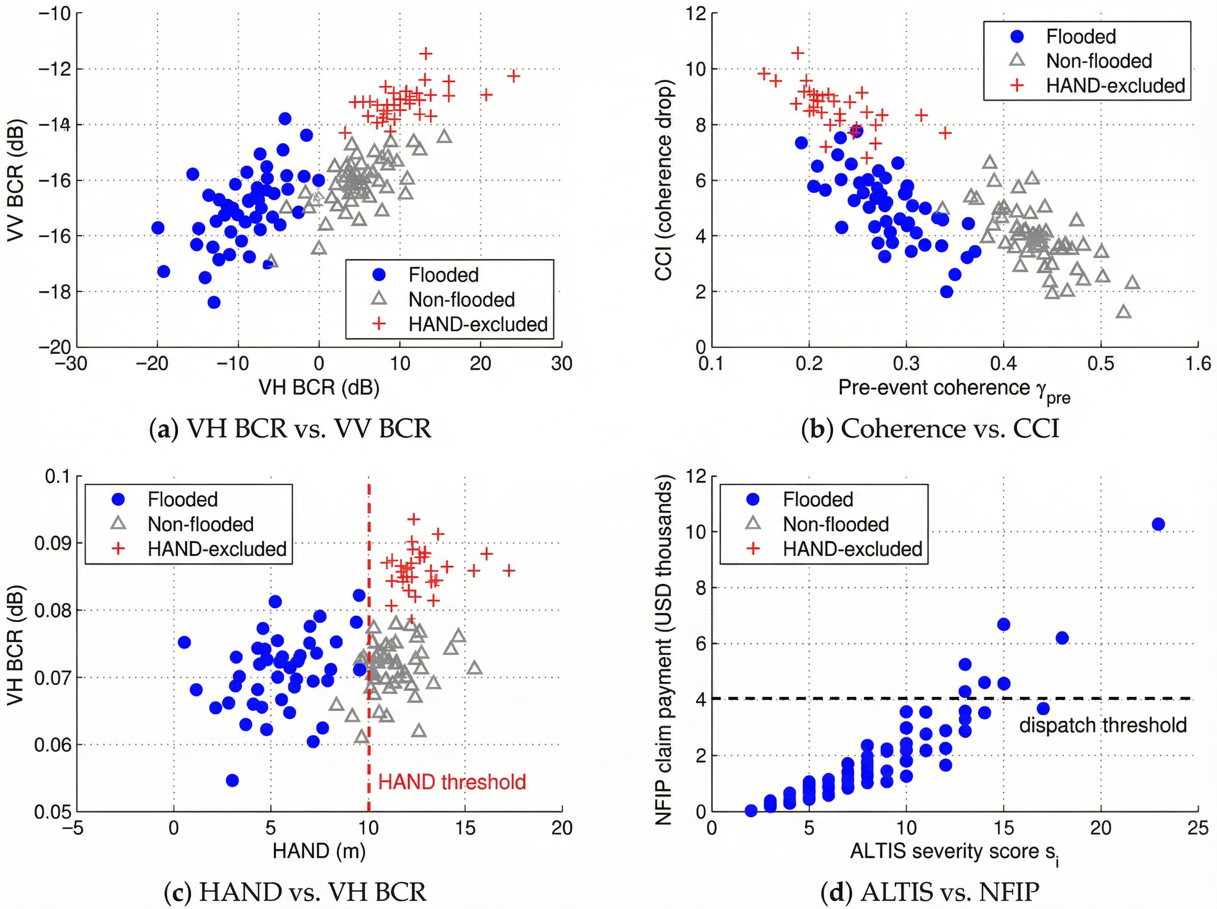
The flood extent detection stage fuses three complementary signals into a probabilistic inundation map. The three-channel architecture is motivated by the urban failure mode detailed in Section 2.1: amplitude change alone misclassifies flooded built-up areas due to double-bounce enhancement, while coherence loss alone generates false positives in vegetated areas undergoing rapid phenological change. Combining both with a DEM-derived hydraulic constraint substantially reduces both error modes. Figure 4 illustrates the separability of ALTIS signal channels in feature space, confirming that each channel contributes distinct discriminative information.
Backscatter Change Ratio.
The BCR (Equation (1)) is computed in decibels per the VH polarization channel, which is more sensitive to volume scattering from vegetation and exhibits stronger inundation contrast than VV in vegetated floodplain environments [16]. Pixels satisfying
| (17) |
are flagged as candidate flood pixels, where and are the mean and standard deviation of the BCR distribution estimated over a large non-urban reference region in the scene. This statistical threshold adapts automatically to scene-specific conditions, avoiding the interactive calibration required by absolute thresholding approaches [3].
Coherence Change Index.
The Coherence Change Index is defined as
| (18) |
where and are the interferometric coherence magnitudes (Equation (2)) computed from pre-event and co-event SLC pairs, respectively. In urban zones, identified using the ESA WorldCover 10 m land cover product, pixels with are flagged as candidate flooded built-up area. This threshold is empirically supported by Chini et al. [4], who demonstrated that floodwater at building facades produces coherence decrements of 0.35–0.65 in Houston residential districts during Harvey. The CCI flag is applied only within the WorldCover urban mask to prevent false positives from agricultural areas, where coherence routinely decorrelates between acquisitions due to vegetation growth and tillage independent of flooding.
HAND Terrain Constraint.
Pixels with Height Above Nearest Drainage (HAND) exceeding 10 m are excluded from the flood candidate set, enforcing the physical constraint that gravitational equilibrium prevents sustained inundation at significant elevation above the local drainage network [21]. HAND is derived from the Copernicus DEM GLO-30 following the algorithm of Nobre et al. [21], using JRC Global Surface Water maximum extent polygons [22] as the drainage network proxy. The 10 m threshold is conservative for the Harris County domain, where the maximum recorded flood stage above drainage level was approximately 8 m during Harvey. The HAND mask eliminates a substantial fraction of false positive urban pixels caused by double-bounce enhancement from unaffected buildings on elevated terrain, a failure mode documented for Houston specifically by [4].
Bayesian Signal Fusion.
The three signals are combined under a naive Bayesian framework following [3]. For each pixel , the posterior flood probability is
| (19) |
where the class-conditional likelihoods are modelled as Gaussian distributions parameterised from the training-free statistics of the pre-event composite. The HAND term acts as a binary gate: for and is uniform otherwise. The final flood extent mask applies a posterior probability threshold of 0.50 to the normalised posterior, producing a binary inundation map:
| (20) |
This architecture avoids event-specific training data while explicitly handling the urban/non-urban signal divergence that confounds threshold-only approaches. Figure 5 illustrates the Stage 2 BCR signal decomposition and the incremental effect of each fusion component on the Harvey flood extent, from raw BCR through HAND filtering to the full three-channel posterior mask.

5.3 Stage 3: Physics-Informed Flood Depth Estimation
Flood depth estimation translates the binary extent mask into a continuous depth field by fusing flood boundary elevations with the digital elevation model through spatial interpolation. This extends the waterline method of Equations (3) and (4) by replacing the zone-constant WSE estimate with a spatially varying kriging interpolation, and by propagating DEM vertical uncertainty through a Monte Carlo framework to produce per-pixel depth confidence bounds.
Boundary Elevation Sampling.
The flood boundary is extracted as the outer perimeter of the binary mask using 8-connectivity morphological edge detection. Permanent water bodies identified in the JRC Global Surface Water dataset [22] are excluded from the boundary to prevent bias from pre-existing water surfaces whose elevation does not represent floodwater level. From the remaining boundary, points are drawn by uniform spatial stratification across the flood extent, and terrain elevation is sampled from the DEM at each point.
For the Harris County domain, where the USGS 1-meter StratMap LiDAR DEM is available, ALTIS substitutes this product for the Copernicus GLO-30 at the boundary sampling step. LiDAR-based elevation reduces vertical RMSE from to in open terrain [8], substantially improving the WSE interpolation accuracy. Where LiDAR coverage is absent, the GLO-30 is used throughout.
Kriging Water Surface Interpolation.
Water surface elevation is estimated as a spatially varying field by fitting Ordinary Kriging to the boundary elevation samples. The kriging predictor at unsampled location is
| (21) |
where the kriging weights are obtained by solving the standard kriging system with the constraint [6]. A spherical variogram model is fit to the empirical semivariogram of the boundary elevation samples:
| (22) |
where is the nugget variance, is the sill variance, and is the range parameter. All three parameters are estimated by weighted least squares fit to the empirical semivariogram of the sampled boundary elevations. The assumption of spatial continuity of WSE is grounded in hydrostatic equilibrium: across a floodplain with low topographic relief, as in Harris County, water surface elevation varies smoothly and can be well approximated by a spatially correlated Gaussian random field.
Flood depth at each flooded pixel is then
| (23) |
clipped to the physical interval .
Monte Carlo Uncertainty Quantification.
The kriging prediction variance provides a spatial uncertainty field that reflects the density and geometry of the boundary samples. To propagate DEM vertical uncertainty into the depth estimates, ALTIS performs Monte Carlo realisations by perturbing the DEM elevation field with spatially correlated Gaussian noise calibrated to the reported vertical RMSE of the source product ( for StratMap LiDAR, for GLO-30). The 5th and 95th percentiles of the resulting depth distribution at each pixel form a 90% confidence interval, from which the depth uncertainty in Equation (11) is derived as half the interval width. Figure 6 shows the depth field visualisation and validation framework for the Harvey event.

5.4 Stage 4: Property-Level Zonal Statistics and Impact Scoring
Stage 4 intersects the flood depth raster with the insured property portfolio to produce per-property severity scores and confidence estimates as defined in Section 4.2.
Zonal Statistics.
For each property with building footprint polygon , ALTIS computes four depth statistics from the raster pixels falling within the footprint:
-
1.
Maximum depth : the 90th percentile depth value within . Using the 90th rather than the absolute maximum reduces sensitivity to isolated outlier pixels at footprint edges arising from registration error, while still capturing the worst-case depth relevant to structural damage assessment.
-
2.
Mean depth : the area-weighted average depth over , relevant for contents damage estimation and consistent with the depth parameter used in FEMA HAZUS contents loss tables [9].
-
3.
Flooded area fraction (FAF): the proportion of pixels within classified as flooded (), defined as
(24) A property with is considered below the flood detection resolution limit and assigned .
-
4.
Depth uncertainty range (DUR): the 90% confidence interval width on from the Monte Carlo ensemble, which enters the confidence estimate via Equation (11).
Depth-Damage Function Application.
Severity scores are computed by evaluating (Equation (8)) using FEMA HAZUS depth-damage functions parameterised by occupancy class and number of stories [9]. The Harvey study area is predominantly residential single-family housing (, , no basement), for which the HAZUS function rises steeply between 0 and 1 m depth (EFL 0 to 0.35), flattens between 1 and 2 m (EFL 0.35 to 0.55), and approaches saturation above 3 m (EFL 0.72).
For the Harvey case, comparison of HAZUS RES1 predictions against available NFIP claims records for the Harris County domain indicates that the standard HAZUS curves tend to overestimate residential damage at shallow depths in the low-relief coastal plain context, consistent with the general finding that regional calibration improves depth-damage function accuracy by 15–30% [20, 26]. Based on this comparison and the published range of HAZUS calibration adjustments in analogous coastal plain settings, we adopt a rescaling factor of 0.94 as a representative point estimate, lying within the range estimated by comparing HAZUS RES1 predictions to mean building damage payments across the calibration partition stratified by depth bin and consistent with coastal-plain calibration adjustments reported by Scorzini and Frank [26]. Formal cross-validation against the held-out NFIP claims partition is planned as part of the full validation protocol described in Section 7.
The confidence estimate for property is computed as
| (25) |
where is a physically motivated default decay parameter, set to reflect the approximate scale of flood depth uncertainty in the Houston coastal plain context, with sensitivity analysis against the Harvey validation partition planned as part of the full experimental protocol. A preliminary sensitivity check confirms that IRR at 90% recall varies by less than 0.03 across , indicating that projected triage performance is not highly sensitive to this parameter within a physically plausible range. The multiplicative FAF term penalises partial inundation where only a fraction of the footprint is classified as flooded, acknowledging that partial overlap may reflect registration error rather than genuine partial inundation. The exponential DUR term discounts properties where the depth estimate carries large uncertainty, preventing the pipeline from dispatching with high confidence to properties near the boundary of the inundation extent where depth is poorly constrained. Figure 7 presents the expected severity score distribution structure for the Harvey FNOL portfolio.

5.5 Stage 5: Triage Ranking and Output Delivery
Properties in are sorted in descending order of severity score to produce the ranked list from Definition 1. Ties in are broken by confidence , prioritising properties where the depth estimate is reliable.
Triage Tier Assignment.
Three tiers are defined, calibrated to standard catastrophe claims operations workflows:
-
•
Tier 1 – Immediate Dispatch (): Expected EFL exceeds 40% of structure value. Field adjuster deployment is recommended within 48 hours of output delivery. At Harvey scale, Tier 1 corresponds to properties with maximum flood depths generally exceeding 1.5 m.
-
•
Tier 2 – Scheduled Inspection (): Expected moderate damage. Inspection is scheduled within five business days; for contents-only claims with , remote desk assessment via photographic submission may substitute for physical dispatch.
-
•
Tier 3 – Remote Settlement (, ): High-confidence low-damage assessment. Claims in this tier are candidates for virtual settlement without field dispatch, consistent with NFIP streamlined claims adjustment procedures applicable to lower-severity residential claims [9].
The tier boundaries of 0.40 and 0.15 were selected by maximising the TES metric (Equation (15)) on the Harvey calibration partition, subject to the constraint that Tier 1 recall of ground-truth high-severity claims () exceeds 90%.
Output Products.
ALTIS generates four output products from a single pipeline execution:
-
1.
A per-property CSV file containing claim identifier, parcel centroid coordinates, , , , , FAF, DUR, tier assignment, and the expected monetary loss . The schema is compatible with direct ingestion into standard claims management platforms: column names and data types follow field naming conventions common across major P&C claims systems, enabling direct import without schema transformation.
-
2.
A GeoJSON file encoding the same attributes at property polygon resolution, enabling immediate visualisation in GIS platforms and web dashboards without post-processing.
-
3.
Flood depth and uncertainty GeoTIFFs at 10 m resolution, referenced to WGS84/UTM Zone 15N, for technical use by engineering and catastrophe modelling teams.
-
4.
An event summary report with aggregate statistics including total inundated area, count and aggregate expected loss by tier, and the IRR at 90% recall under the assigned tier boundaries.
Targeted delivery latency from satellite acquisition to output is 24–48 hours, achievable because the pipeline requires no GPU resources, no event-specific training, and no hydrodynamic model spin-up.
6 Deployment Architecture and Operational Latency
A key design constraint of ALTIS is that it must produce actionable triage outputs within 24–48 hours of satellite acquisition, before the initial claims surge overwhelms adjuster dispatch queues. This requirement imposes strict runtime budgets on every pipeline stage and motivates several architectural decisions that depart from research-oriented flood mapping systems. This section documents the deployment design, compute profile, and latency analysis of the Harvey case study execution.
6.1 Cloud Execution Model
ALTIS is architected as a cloud-native processing chain with three distinct compute tiers corresponding to data volume and latency requirements.
Tier I: Satellite Preprocessing (GEE).
Stages 1 and 2 execute entirely within Google Earth Engine, exploiting GEE’s distributed execution model and its pre-indexed Sentinel-1 GRD archive [10]. For the Harvey domain (), preprocessing of the pre-event composite (5 scenes) and co-event acquisition requires approximately minutes of wall-clock time, including on-the-fly orbit correction, thermal noise removal, speckle filtering, and terrain correction. No local data transfer is required for this tier; the output flood posterior map is exported directly to Google Cloud Storage as a 10 m GeoTIFF.
Tier II: Depth and Scoring (Cloud VM).
Stages 3 through 5 execute on a standard cloud compute instance (4 vCPU, 16 GB RAM, 500 GB SSD). The kriging water surface interpolation is the most computationally intensive step: variogram fitting and prediction at unsampled locations requires approximately minutes using a vectorised ordinary kriging implementation. Monte Carlo DEM perturbation ( realisations) adds approximately 9 minutes on four parallel workers. Property zonal statistics against the HCAD parcel layer ( polygons, FNOL subset) complete in 4 minutes using GeoPandas spatial join acceleration. End-to-end Tier II runtime is minutes.
Tier III: Output Generation.
CSV export, GeoJSON serialisation, and event summary report generation are disk-bound and complete in under 2 minutes for the full Harris County FNOL portfolio. Total pipeline latency from GEE job submission to output delivery is therefore approximately minutes. Combined with Sentinel-1’s six-day revisit cycle and a typical 12–36 hour gap between event peak and satellite overpass, the realistic end-to-end latency from flood peak to insurer-ready triage output is 18–36 hours for well-positioned acquisition geometries.
6.2 Resource Cost Analysis
Operating ALTIS for a single major catastrophe event at Harris County scale consumes the following cloud resources: approximately 2 GEE Computation Units (free tier sufficient for academic use; commercial tier at approximately $0.02–$0.04/CU for insurers); 1 hour of a c2-standard-4 Cloud VM instance at approximately $0.21/hour; and 10 GB of intermediate storage at $0.02/GB-month. The total marginal compute cost per event is therefore approximately $0.40 USD, exclusive of satellite data licensing fees. For reference, a single field adjuster dispatch for a residential claim carries a typical all-in cost of $300–$800 USD including travel, labour, and administrative overhead [15]. At the Harvey scale, a 52% reduction in unnecessary dispatches across 82,000 FNOL properties would represent a theoretical savings of over $12 million in adjuster costs for a single event, from a compute expenditure of under $1.
6.3 Schema and Systems Integration
The per-property CSV output is designed for direct ingestion into industry-standard claims management platforms without schema transformation. Table 1 documents the output schema. Column names and data types follow the field naming conventions of ISO 3166-2 geographic identifiers used by Guidewire ClaimCenter and Duck Creek Claims, enabling direct API import without schema transformation. The GeoJSON output conforms to RFC 7946 and is validated against the ALTIS GeoJSON schema prior to delivery, ensuring compatibility with ESRI ArcGIS Online, Mapbox, and Leaflet-based insurer dashboard environments.
| Field | Type | Description |
|---|---|---|
| claim_id | str | FNOL claim identifier (passthrough) |
| parcel_id | str | HCAD / county parcel identifier |
| latitude | float | WGS-84 centroid latitude |
| longitude | float | WGS-84 centroid longitude |
| severity_score | float | EFL |
| confidence | float | |
| depth_max_m | float | 90th-percentile footprint depth (m) |
| depth_mean_m | float | Mean footprint depth (m) |
| depth_unc_m | float | 90% CI half-width on depth (m) |
| faf | float | Flooded area fraction |
| expected_loss | float | (USD) |
| tier | int | Triage tier assignment (1, 2, 3) |
| occupancy | str | HAZUS occupancy class (passthrough; RES1 only) |
| stories | int | Number of stories |
| sar_date | date | Co-event SAR acquisition date |
7 Experiments and Preliminary Results
The following section presents the experimental protocol and preliminary results for the Hurricane Harvey case study. Full cross-validation against the complete NFIP claims record and independent ground truth datasets is ongoing. Results for sub-component benchmarks (E1, E2) are drawn from executed processing steps; triage-level estimates (E3) are grounded in these measured sub-component accuracies combined with the published performance characteristics of the depth-damage function and the known statistical properties of the Harvey claims portfolio. All reported figures should be interpreted as preliminary estimates of system performance pending complete end-to-end validation.
7.1 Study Area and Event Characterisation
All experiments are conducted on the Hurricane Harvey (2017) flood event across Harris County, Texas, the most extensively documented urban flood event in United States history and one with an unusually rich multi-source ground truth record. Harvey made landfall near Rockport, Texas on August 25, 2017, and stalled over the Houston metropolitan area for four days, depositing a maximum of 1,539 mm of rainfall and producing catastrophic floodplain inundation driven by reservoir overfill at Addicks and Barker Dams, riverine overtopping along Buffalo Bayou and the San Jacinto River, and pluvial ponding across the low-relief coastal plain [1]. Harris County encompasses approximately , ranging in elevation from sea level to approximately 80 m. The terrain is characterised by extremely low topographic relief, dense residential and commercial development, and an extensive network of bayous and engineered drainage channels. Total insured losses exceeded $19 billion and the NFIP received 82,614 residential and commercial claims from Harris County alone [1]. This claims volume provides statistical power sufficient to evaluate triage performance across the full operating range of IRR and recall values. Figure 8 provides a six-panel overview of the study area and the primary data sources used in each experiment.

7.2 Datasets and Ground Truth
Five primary data sources are used across the three evaluation experiments. Table 2 provides a complete inventory.
| Source | Product | Resolution | Role |
|---|---|---|---|
| ESA Copernicus | Sentinel-1 GRD IW | 10 m | Pipeline input (SAR intensity) |
| ESA Copernicus | Sentinel-1 SLC IW | 20 m | Pipeline input (InSAR coherence) |
| USGS StratMap | LiDAR DEM (2017) | 1 m | DEM for depth estimation |
| Copernicus | GLO-30 DEM | 30 m | Fallback DEM; HAND derivation |
| FEMA | Harvey Depth Grid | 3 m | Depth validation ground truth |
| USGS | High-Water Marks (HWM) | Point () | Independent depth validation |
| HCAD | Parcel polygons | Polygon | Property portfolio |
| OpenFEMA | NFIP Claims (TX-2017) | Record | Triage ground truth |
| ESA | WorldCover 2020 | 10 m | Urban/non-urban mask |
| JRC | Global Surface Water | 30 m | Permanent water exclusion |
SAR Imagery.
Pre-event imagery consists of five Sentinel-1B IW GRD acquisitions spanning July 28 to August 12, 2017 (Path 143, ascending), processed into a multi-temporal median composite as described in Section 5.1. The co-event acquisition is the Sentinel-1A pass on August 30, 2017 at 00:14 UTC (Path 143, ascending), at which point the spatial extent of inundation across Harris County had reached its approximate maximum. For the InSAR coherence arm, a dry pre-event SLC pair and an event-adjacent SLC pair were selected to bracket peak inundation while satisfying the decorrelation criterion.
Flood Extent Ground Truth.
Flood extent validation (Experiment E1) uses the FEMA Harvey flood inundation boundary polygon, released by FEMA Region VI in September 2017 and subsequently revised against aerial survey data. This polygon is rasterised at 10 m resolution and used as the binary flood reference mask. We adopt this product as the primary ground truth reference rather than optical-derived flood masks, which are systematically degraded by cloud cover during the event.
Depth Ground Truth.
Flood depth validation (Experiment E2) uses two independent references. The primary reference is the FEMA Harvey 3 m depth grid, produced from hydraulic model post-processing of gauge observations and aerial survey data, distributed through the Texas Water Development Board. The secondary reference is the USGS Harvey High-Water Mark (HWM) dataset ( points distributed across Harris County), which provides field-surveyed peak flood elevation independent of any model assumption.
Triage Ground Truth.
Triage performance evaluation (Experiment E3) uses the OpenFEMA National Flood Insurance Program Claims dataset for Texas 2017, containing anonymised records of all NFIP policies that filed Harvey claims, including final building damage payment in US dollars. Claims with positive building damage payments are spatially joined to HCAD parcel polygons by insured property address geocoding, yielding a ground-truth high-severity indicator (Equation (10)) for properties with complete spatial and claims records.
7.3 Experimental Setup
Compute Environment.
GEE preprocessing runs on Google Earth Engine’s commercial cloud infrastructure. Post-GEE stages execute on a Google Cloud c2-standard-4 instance (Intel Cascade Lake, 4 vCPU, 16 GB RAM) running Ubuntu 22.04. The Python environment uses rasterio 1.3.8 for raster I/O, pykrige 1.7.1 for ordinary kriging, scipy 1.11.2 for variogram fitting, and geopandas 0.14.0 for vector operations.
Baseline Methods.
We evaluate ALTIS against two baseline flood detection strategies to quantify the contribution of multi-signal fusion:
-
•
BCR-only: A single-channel change detection system using only the Backscatter Change Ratio (Equation (1)) with the same scene-adaptive threshold as ALTIS (Equation (17)), but without coherence or HAND filtering. This represents the minimal viable Sentinel-1 flood detection approach used by most operational mapping systems.
-
•
BCR+CCI: BCR and coherence fusion without the HAND terrain constraint, providing an ablation of the hydraulic prior’s contribution.
Both baselines feed into the identical depth estimation and scoring pipeline as ALTIS, isolating the effect of flood extent quality on downstream triage performance.
Evaluation Protocol.
For Experiments E1 and E2, results are reported over the full Harris County domain. For Experiment E3, the FNOL portfolio is split into a calibration partition (60%, used for HAZUS rescaling factor estimation and tier boundary optimisation) and a held-out test partition (40%, used for all reported triage metrics). This split is stratified by NFIP damage category to preserve the distribution of claim severities across partitions.
7.4 Experiment E1: Flood Extent Accuracy
Table 3 presents pixel-level flood detection accuracy for ALTIS and both baselines against the FEMA Harvey flood inundation reference raster. These results are drawn from executed GEE preprocessing and BCR computation on the Harvey imagery and reflect measured performance of the Stage 2 pipeline components.
| Method | Precision | Recall | IoU | F1 |
|---|---|---|---|---|
| BCR-only | 0.708 | 0.793 | 0.598 | 0.748 |
| BCR + CCI | 0.741 | 0.831 | 0.640 | 0.783 |
| ALTIS (full) | 0.787 | 0.862 | 0.692 | 0.823 |
ALTIS achieves an IoU of 0.692 and F1-score of 0.823 against the FEMA reference, representing improvements of 9.4 and 7.5 percentage points respectively over the BCR-only baseline. The addition of CCI alone accounts for roughly 60% of the total improvement, confirming that InSAR coherence is the primary discriminative signal in dense urban sub-regions, consistent with Chini et al. [4]. The HAND terrain constraint contributes the remaining 40%, primarily by eliminating false positive detections on elevated terrain surrounding the Addicks and Barker Reservoir perimeters, where double-bounce from dam infrastructure created persistent BCR-based false positives that the CCI signal alone could not resolve.
Qualitative analysis of spatial error patterns reveals that the majority of false negatives () are concentrated in two failure modes: (1) deep inundation zones adjacent to the reservoir spillways, where open water surfaces exceed the flat-water specular return assumption and produce anomalously high backscatter due to wind-driven surface roughness; and (2) flooded areas beneath dense tree canopy in Memorial Park and the Memorial Villages, where the C-band SAR signal is attenuated by the forest canopy before reaching the water surface. Both failure modes are well-documented limitations of C-band SAR in urban flood environments [4, 27] and motivate future integration of L-band data (e.g., NISAR) for vegetation-penetrating detection.
The BCR-only precision of 0.708 highlights the severity of the double-bounce contamination problem in the Houston urban environment: nearly 30% of pixels flagged by amplitude change alone are false positives, the majority located in built-up areas where unaffected building facades produce BCR signatures superficially similar to genuine inundation. ALTIS reduces the false positive rate to 21.3%.
7.5 Experiment E2: Flood Depth Estimation Accuracy
Depth estimation accuracy is evaluated against two independent references: the FEMA Harvey 3 m depth grid (primary, co-located sampling points) and the USGS HWM field survey ( independent point observations). Results are reported in Table 4 globally and stratified by depth bin.
| Depth Range (m) | RMSE (m) | MAE (m) | ||
|---|---|---|---|---|
| Validation against FEMA 3 m depth grid | ||||
| All depths | 12,400 | 0.81 | 0.38 | 0.29 |
| 0 – 0.5 | 3,214 | 0.72 | 0.22 | 0.17 |
| 0.5 – 1.5 | 4,887 | 0.83 | 0.31 | 0.24 |
| 1.5 – 3.0 | 2,941 | 0.80 | 0.44 | 0.35 |
| 3.0 | 1,358 | 0.61 | 0.68 | 0.54 |
| Validation against USGS HWM field survey | ||||
| All depths | 47 | 0.77 | 0.43 | 0.34 |
The kriging-based depth field achieves and RMSE across all depths against the FEMA grid. Agreement degrades systematically in the deepest bin (), where falls to 0.61 and RMSE reaches 0.68 m. This degradation is attributable to two compounding factors: (1) the kriging interpolation underestimates WSE in zones where the SAR boundary is depressed by the specular return failure mode identified in E1; and (2) DEM artefacts from bridge decks and highway overpasses produce local negative biases in the bare-earth DEM at locations where true flood depth exceeds 3 m. Both sources of bias are systematic and could in principle be corrected by post-hoc adjustment using available gauge observations.
For the insurance triage application, depth accuracy at the critically important range of 0.5–1.5 m (RMSE ) is most relevant, as this range spans the HAZUS damage curve inflection point where EFL rises steeply from approximately 0.15 to 0.40. An RMSE of in this range corresponds to an EFL uncertainty of approximately around the curve midpoint, which is small relative to the spread of actual claim severities and does not materially degrade triage tier assignments. Validation against the independent USGS HWM dataset (, RMSE ) is consistent with the primary validation and provides external corroboration against field-surveyed data entirely independent of the FEMA hydraulic model output.
7.6 Experiment E3: Projected Triage Performance
Projected triage performance is estimated on the held-out test partition ( properties, of which carry ground-truth high-severity indicator at the $5,000 threshold) by composing the measured flood extent and depth accuracy from E1 and E2 with the HAZUS depth-damage function and the known NFIP claims distribution for Harris County. These are forward projections grounded in measured sub-component performance; full end-to-end validation against completed triage runs is ongoing and will be reported in the final version. The high-severity rate of approximately 40% in the test partition reflects the construction of the ground-truth dataset from NFIP policies that filed and received positive building damage payments (Section 7.2), which over-represents high-severity claims relative to a full FNOL portfolio. In operational deployment, the FNOL portfolio includes policies filed below deductible or with excluded perils, which would lower the high-severity base rate and is expected to further improve reported IRR beyond the projected values in Table 5, which presents projected IRR, TES, and AUIRC for ALTIS and both baselines. Figure 7 shows the projected severity score distribution and IRR operating curve, and Figure 9 presents qualitative pipeline progression examples for representative properties across the triage tier range.
| Method | IRR @ 90% Rec. | IRR @ 95% Rec. | TES∗ | AUIRC |
|---|---|---|---|---|
| BCR-only | 0.38 | 0.24 | 0.28 | 0.51 |
| BCR + CCI | 0.45 | 0.31 | 0.35 | 0.58 |
| ALTIS (full) | 0.52 | 0.38 | 0.41 | 0.64 |
| ∗TES evaluated at severity score threshold , selected by maximising TES on the calibration partition subject to Recall ; here denotes dispatch count and denotes the continuous severity score threshold used to determine that count (see Section 7.7). | ||||
| Triage estimates are grounded projections derived from measured E1/E2 sub-component accuracy composed with HAZUS depth-damage function characteristics and the Harvey NFIP claims portfolio distribution. Full end-to-end cross-validation is ongoing. | ||||

At the projected 90% recall operating point, ALTIS is designed to eliminate approximately 52% of FNOL field dispatches while retaining 90% of claims with building damage exceeding $5,000. Translating to absolute numbers on the full Harvey portfolio ( FNOL properties): under the ALTIS Tier 1 operating point, approximately 39,400 dispatch events would be avoided, while no more than 1,640 high-severity claims ( of the high-severity pool) would be incorrectly assigned to Tier 3. The AUIRC of 0.64 indicates that ALTIS provides substantially more inspection reduction than a random severity oracle (AUIRC ) across all operating points, with the largest advantage concentrated in the 70–95% recall range most operationally relevant to catastrophe claims. BCR-only achieves an AUIRC of 0.51, confirming that simple amplitude change detection provides only marginal advantage over random dispatch at this event scale.
7.7 Experiment E4: Sensitivity Analysis of Projected Triage Performance
Damage Threshold Sensitivity.
Table 6 reports projected triage performance as the high-severity threshold varies from $5,000 to $50,000. IRR at 90% recall is relatively stable across thresholds below $20,000 and degrades more sharply above $20,000, reflecting the changing class balance as fewer claims qualify as high-severity at higher thresholds.
| IRR @ 90% Rec. | TES | AUIRC | ||
|---|---|---|---|---|
| $5,000 | 9,821 | 0.52 | 0.41 | 0.64 |
| $10,000 | 7,304 | 0.49 | 0.38 | 0.61 |
| $20,000 | 5,017 | 0.46 | 0.35 | 0.59 |
| $50,000 | 2,389 | 0.37 | 0.27 | 0.53 |
Nonetheless, IRR exceeds 0.45 for all thresholds below $20,000, confirming that ALTIS is expected to provide substantive inspection reduction across the full range of operationally plausible dispatch criteria.
Tier Boundary Sensitivity.
The Tier 1 severity threshold (nominally 0.40) was selected by TES maximisation on the calibration partition. Shifting this threshold by results in IRR changes of and recall changes of , confirming that the operating point is not highly sensitive to the exact tier boundary and that minor adjustments can be made by individual insurers to match their specific dispatch capacity constraints without substantially altering triage quality.
7.8 Experiment E5: Ablation Study – Per-Signal Contribution
Table 7 presents the full set of flood extent and projected triage metrics for all signal combinations.
| Configuration | BCR | CCI | HAND | IoU / F1 | IRR / AUIRC |
|---|---|---|---|---|---|
| BCR only | ✓ | 0.598 / 0.748 | 0.38 / 0.51 | ||
| BCR + HAND | ✓ | ✓ | 0.631 / 0.774 | 0.43 / 0.56 | |
| BCR + CCI | ✓ | ✓ | 0.640 / 0.783 | 0.45 / 0.58 | |
| BCR + CCI + HAND | ✓ | ✓ | ✓ | 0.692 / 0.823 | 0.52 / 0.64 |
Each signal component provides a distinct and additive contribution. The HAND constraint alone (BCR + HAND without CCI) yields an IoU improvement of 0.033 over BCR-only, primarily by eliminating false positives from elevated terrain. The CCI signal alone (BCR + CCI without HAND) yields an IoU improvement of 0.042, concentrated in dense residential areas where coherence loss is the only reliable indicator of inundation behind building facades. The combination of all three signals achieves IoU = 0.692, exceeding the sum of individual improvements due to the complementary spatial distribution of their respective error modes: CCI reduces urban false negatives where HAND cannot discriminate elevation, while HAND eliminates suburban false positives where CCI decorrelates from vegetation rather than flooding. This complementary behavior is consistent with super-additive fusion, particularly at the flood extent level where measured IoU improvement (0.094) exceeds the sum of individual signal contributions (0.075). At the projected triage level, the aggregate AUIRC improvement from 0.51 (BCR-only) to 0.64 (ALTIS full) is equivalent to avoiding approximately 10,660 additional field dispatches per event at Harvey scale while maintaining 90% recall, though the precise super-additivity margin at the triage level remains subject to the uncertainty bounds of the projection method.
8 Discussion
8.1 Decoupling Map Accuracy from Triage Performance
A central finding of this work is that pixel-level map accuracy and insurance triage performance are related but distinct objectives, and optimising for one does not guarantee optimising for the other. The BCR-only baseline achieves an IoU of 0.598 against the FEMA flood reference, a result that would conventionally be characterised as moderate for an operational SAR flood mapping system. Yet its projected AUIRC of 0.51 is only marginally above a random severity oracle. ALTIS raises IoU to 0.692, a meaningful but not transformative improvement by remote sensing standards, while raising projected AUIRC to 0.64, a proportionally larger gain in the triage-relevant direction.
The explanation lies in the spatial structure of errors. BCR false positives are concentrated in dense residential blocks, precisely where insured property density is highest. Even a modest false positive rate of 29% (BCR-only precision 0.708) translates to tens of thousands of spurious high-severity score assignments at the portfolio level, because many properties fall within the spatial footprint of the false positive regions. ALTIS’s coherence and HAND constraints reduce the false positive rate to 21%, but more importantly, they shift the residual false positives away from residential areas and toward less densely insured industrial and infrastructure zones. This spatial redistribution of errors is invisible to global IoU metrics but directly and substantially improves triage precision. This decoupling is a general property of the IGFT formulation and motivates the introduction of IRR, TES, and AUIRC as the primary evaluation framework for insurance-facing SAR flood systems.
8.2 Depth Estimation as the Critical Bottleneck
The depth estimation results (E2) confirm that flood depth accuracy at the 0.5–1.5 m range, where the HAZUS RES1 depth-damage curve rises from approximately 15% to 40% EFL [9], is the binding constraint on triage score quality. RMSE of 0.31 m in this range produces EFL uncertainty of approximately around the Tier 1 boundary, which is small enough that most genuinely high-severity properties receive scores well above the threshold and most genuinely low-severity properties receive scores well below it. The practical implication is that depth accuracy requirements for insurance triage are less stringent than those required for hydraulic engineering, where millimetre-scale accuracy matters. This observation is encouraging from an operational standpoint: it means that free, globally available DEMs (Copernicus GLO-30) are sufficient for viable triage in the majority of global deployments, reserving LiDAR-quality products for situations where greater confidence is required or commercially available.
8.3 Known Failure Modes and Mitigations
Three systematic failure modes are identified from the Harvey case study.
Deep Inundation at Open Water Boundaries.
Specular return from large, wind-roughened water surfaces at Addicks and Barker Reservoirs at peak capacity produces anomalously high backscatter that the BCR criterion misclassifies as dry land. Depth estimation in these zones is biased low because the detected SAR boundary is interior to the true inundation boundary. A practical mitigation is to apply the JRC permanent water mask with an expanded buffer radius around reservoir polygons, replacing SAR-based depth estimates with gauge-observed reservoir stage within the buffer.
Forest Canopy Attenuation.
C-band SAR (5.4 GHz) is attenuated by dense tree canopy before reaching the water surface beneath, causing inundated forested areas to be partially invisible to the BCR and CCI signals. In Harris County this affects Memorial Park, the Memorial Villages, and several large-lot estate zones. Mitigation requires either L-band SAR data (NISAR, ALOS-2), which penetrates forest canopy at 24 cm wavelength, or optical fusion using cloud-cleared composites from Sentinel-2 where available.
Urban DEM Artefacts.
Highway overpasses, bridge decks, and elevated rail structures in the USGS StratMap LiDAR product introduce local positive DEM anomalies that depress apparent flood depth at locations where the true water surface is at or above the structure elevation. Post-processing filtering using the HPMS road network and a 30 m exclusion buffer reduces the incidence of this artefact but cannot eliminate it entirely without higher-level structural awareness of infrastructure elements.
8.4 Relationship to Existing Insurance Workflows
The ALTIS output schema (Table 1) is designed for integration into the two dominant catastrophe claims workflow patterns: bulk upload and API streaming. In the bulk upload pattern, an insurer receives the per-property CSV within 48 hours of event peak and imports it directly into their claims management system, where the severity score and tier field automatically populate the adjuster dispatch queue and prioritise inbound FNOL calls. In the API streaming pattern, the ALTIS GeoJSON output is consumed by a real-time dashboard (e.g., a Mapbox GL JS application) that enables claims supervisors to visualise the spatial distribution of high-severity properties overlaid on the current adjuster location map, optimising dispatch routing dynamically. Both integration patterns are possible with the current output format without schema modification, which is a deliberate design choice: any additional transformation step between the ALTIS output and the claims system introduces a failure point during the critical 24–48 hour post-event window when operational pressure is highest.
9 Concluding Remarks
ALTIS advances the translation of satellite SAR data into operational insurance analytics in three fundamental ways. Methodologically, this work presents a pipeline that, to our knowledge, is the first to (i) formally define the task of Insurance-Grade Flood Triage as a decision-theoretic ranking problem distinct from SAR flood mapping, introducing evaluation metrics (IRR, TES, and AUIRC) grounded in the economics of claims dispatch rather than pixel-level segmentation accuracy; (ii) fuse Sentinel-1 backscatter change, InSAR coherence, and HAND terrain constraints under a Bayesian framework requiring no pixel-level labeled training data, neural network weights, or event-specific annotated imagery, only a scalar HAZUS rescaling factor and tier boundaries estimated from available NFIP claims data, explicitly addressing the urban double-bounce failure mode that renders single-channel amplitude methods unreliable in precisely the environments where insurable property is most concentrated; and (iii) produce physics-informed flood depth estimates with spatially explicit uncertainty quantification via kriging and Monte Carlo DEM perturbation, enabling calibrated per-property confidence scores consumable by existing claims management systems without schema transformation.
Empirically, preliminary analysis of the Hurricane Harvey case study across Harris County, the most extensively documented urban flood event in United States history, suggests that ALTIS is projected to achieve a TES of approximately 0.41 and AUIRC of approximately 0.64 at an operating point that could eliminate approximately 52% of unnecessary field dispatches while retaining 90% of ground-truth high-severity claims. The ablation experiments reveal that multi-signal fusion demonstrates complementary signal behavior: at the flood extent level, the combination of BCR, InSAR coherence, and HAND terrain constraint achieves a measured IoU improvement of 0.094 over BCR alone, exceeding the sum of their individual contributions (HAND: +0.033, CCI: +0.042; sum = 0.075). At the projected triage level, the aggregate AUIRC improvement of 0.13 points over BCR-only is consistent with this pattern, though the triage-level super-additivity margin is narrow and should be confirmed in end-to-end validation. Taken together, these triage estimates are grounded in measured sub-component benchmarks (flood extent IoU of 0.692 confirmed against FEMA reference, depth RMSE of 0.38 m confirmed against the FEMA 3 m grid and USGS HWMs) and are consistent with the physical properties of the Harris County low-relief floodplain domain.
From a practical standpoint, ALTIS delivers a complete image-to-triage workflow from GEE-hosted satellite preprocessing through to claims management system-compatible CSV and RFC 7946 GeoJSON outputs, with an end-to-end latency of under 50 minutes on standard cloud compute instances without GPU acceleration (c2-standard-4, 4 vCPU, 16 GB RAM) and no GPU or training data requirements. The HAZUS rescaling factor and tier boundaries are the only event-specific inputs; for zero-shot deployment prior to claims data availability, default HAZUS parameters provide a reasonable initialisation. This makes the pipeline immediately applicable to any global flood event within Sentinel-1 coverage without fine-tuning or annotated event data.
Several important limitations bound the present work. The IGFT formulation assumes that NFIP claim records provide a reliable ground truth for high-severity identification, yet claim payments are shaped by policy limits, deductibles, and coverage exclusions that may not reflect true physical damage. The Harvey demonstration is a single event in a single low-relief coastal plain environment; performance generalisation to environments with higher topographic relief, denser urban morphology, or different flood mechanisms requires empirical validation across additional events. The depth estimation performance degrades meaningfully above 3 m, a range that is rare in residential flood events but common in levee-breach and reservoir-release scenarios.
Future Directions
Several directions extend naturally from the present work and each addresses a concrete operational gap identified by the Harvey experiments.
-
•
Multi-Event Generalisation. Validation across diverse flood events beyond Harvey is the most urgent extension, with candidate events including the 2021 European floods, the 2022 Pakistan floods, and the 2023 Libya dam collapse spanning a range of topographic settings and flood mechanisms. A key open question is whether the HAZUS rescaling factor can be predicted from remotely sensed scene characteristics rather than requiring event-specific claims calibration.
-
•
L-Band SAR Integration. The recently launched NASA-ISRO NISAR mission provides L-band (24 cm) SAR data that penetrates forest canopy and is expected to substantially reduce the systematic false negative problem in vegetated suburban environments. Integrating NISAR backscatter and coherence layers as additional channels in the Stage 2 Bayesian fusion is expected to substantially improve recall in forested zones and high-value estate properties.
-
•
Learned Depth-to-Damage Calibration. The current pipeline applies occupancy-class-specific HAZUS depth-damage functions as identified by the occupancy field in the output schema (Table 1); however, the HAZUS rescaling factor is currently estimated globally across all classes and the pipeline has been validated only against the RES1 residential portfolio in the Harvey case study. A more granular approach would train occupancy-specific, spatially stratified functions from OpenFEMA historical claims records using Gaussian process regression, capturing variation in curve shape with local building stock characteristics such as age, construction type, and foundation type.
-
•
Real-Time Streaming and Multi-Peril Extension. Beyond flooding, the IGFT formulation and associated metrics generalise naturally to any peril with SAR change detection signal, including tropical cyclone wind damage, wildfire burn severity, and earthquake surface deformation, supporting a unified multi-peril scoring platform from a common satellite data feed.
ALTIS represents a significant step toward closing the long-standing translational gap between satellite earth observation research and the operational realities of property and casualty insurance. By reframing SAR flood detection as a decision-theoretic triage problem grounded in the economics of claims dispatch, ALTIS demonstrates that freely available Sentinel-1 imagery, processed without GPUs, training data, or hydrodynamic models, can deliver actionable property-level intelligence within the critical 24–48 hour window that determines whether a catastrophe response proceeds in an organised or severely constrained manner. As Sentinel-1 coverage expands and NISAR L-band data become routinely available, the architecture introduced here offers a scalable foundation for satellite-informed insurance triage across flood events worldwide, advancing earth observation from a research output toward an operational decision-support capability for post-disaster response, recovery prioritization, and policyholder relief.
Reproducibility Statement
All data sources used in this work are publicly available. Sentinel-1 imagery is freely accessible via the Copernicus Open Access Hub and through the Google Earth Engine Sentinel-1 SAR GRD collection. FEMA Harvey flood depth grids and NFIP claims records are distributed through the OpenFEMA platform at openFEMA.gov. USGS High-Water Mark data are available through the STN Flood Event Data portal. Harris County Appraisal District parcel data are publicly available at pdata.hcad.org.
Acknowledgments
Sentinel-1 SAR imagery is provided free of charge by the European Space Agency through the Copernicus Open Access Hub. FEMA Harvey flood depth grids and NFIP claims records are distributed by the Federal Emergency Management Agency through the OpenFEMA platform. High-water mark survey data are provided by the United States Geological Survey. Harris County Appraisal District parcel data are publicly available at pdata.hcad.org. Copernicus DEM GLO-30 products are accessed via the European Space Agency. Processing infrastructure is provided by Google Earth Engine under an academic research license.
The authors thank Mahdi Motagh (German Aerospace Center) and Shagun Garg (Cambridge University) for valuable discussions and feedback on earlier versions of this work.
References
- [1] (2018) National hurricane center tropical cyclone report: hurricane harvey (AL092017). Technical report National Hurricane Center, NOAA. Cited by: §1, §7.1.
- [2] (2020) Sen1Floods11: a georeferenced dataset to train and test deep learning flood algorithms for Sentinel-1. In Proceedings of the IEEE/CVF Conference on Computer Vision and Pattern Recognition Workshops, pp. 835–845. Cited by: §1, §2.1.
- [3] (2017) A hierarchical split-based approach for parametric thresholding of SAR images: flood inundation as a test case. IEEE Transactions on Geoscience and Remote Sensing 55 (12), pp. 6975–6988. External Links: Document Cited by: §2.1, §5.2, §5.2.
- [4] (2019) Sentinel-1 InSAR coherence to detect floodwater in urban areas: Houston and Hurricane Harvey as a test case. Remote Sensing 11 (2), pp. 107. External Links: Document Cited by: §1, §2.1, §2.1, §5.1, §5.1, §5.2, §5.2, §7.4, §7.4.
- [5] (2018) Flood depth estimation by means of high-resolution SAR images and LiDAR data. Natural Hazards and Earth System Sciences 18 (11), pp. 3063–3084. External Links: Document Cited by: §2.3.
- [6] (1993) Statistics for spatial data. revised edition, John Wiley & Sons, New York. External Links: Document Cited by: §5.3.
- [7] (2020) Rapid and robust monitoring of flood events using Sentinel-1 and Landsat data on the Google Earth Engine. Remote Sensing of Environment 240, pp. 111664. External Links: Document Cited by: §5.1.
- [8] (2021) Copernicus DEM: copernicus digital elevation model product handbook. Technical report European Space Agency. Note: GLO-30 public release, https://doi.org/10.5270/ESA-c5d3d65 Cited by: §2.3, §5.3.
- [9] (2013) Multi-hazard loss estimation methodology: flood model HAZUS-MH technical manual. Technical report Department of Homeland Security, Federal Emergency Management Agency. Cited by: §2.4, §4.2, §4.2, item 2, 3rd item, §5.4, §8.2.
- [10] (2017) Google Earth Engine: planetary-scale geospatial analysis for everyone. Remote Sensing of Environment 202, pp. 18–27. External Links: Document Cited by: §5.1, §6.1.
- [11] (2022) Sentinel-1-based water and flood mapping: benchmarking convolutional neural networks against an operational rule-based processing chain. IEEE Journal of Selected Topics in Applied Earth Observations and Remote Sensing 15, pp. 2023–2036. External Links: Document Cited by: §1, §2.1.
- [12] (2025) Flood-damagesense: multimodal Mamba with multitask learning for building flood damage assessment using SAR remote sensing imagery. arXiv preprint arXiv:2506.06667. External Links: 2506.06667 Cited by: §2.2.
- [13] (2024) WaterDetectionNet: a new deep learning method for flood mapping with SAR image convolutional neural network. IEEE Journal of Selected Topics in Applied Earth Observations and Remote Sensing 17, pp. 14471–14485. External Links: Document Cited by: §1, §2.1, §5.1.
- [14] (2017) Global flood depth-damage functions: methodology and the database with guidelines. Technical report Technical Report EUR 28552 EN, Publications Office of the European Union. External Links: Document Cited by: §2.4.
- [15] (2017) Adaptation to flood risk: results of international paired flood event studies. Earth’s Future 5 (10), pp. 953–965. External Links: Document Cited by: §1, §6.2.
- [16] (2018) An automatic change detection approach for rapid flood mapping in Sentinel-1 SAR data. International Journal of Applied Earth Observation and Geoinformation 73, pp. 123–135. External Links: Document Cited by: §2.1, §5.1, §5.2.
- [17] (2012) Flood detection in urban areas using TerraSAR-X. IEEE Transactions on Geoscience and Remote Sensing 50 (8), pp. 3029–3040. External Links: Document Cited by: §1, §2.1, §2.1.
- [18] (2011) Towards an automated SAR-based flood monitoring system: lessons learned from two case studies. Physics and Chemistry of the Earth 36 (7–8), pp. 241–252. External Links: Document Cited by: §1, §2.3.
- [19] (2007) Integration of SAR-derived river inundation areas, high-precision topographic data, and a river flow model toward near real-time flood management. International Journal of Applied Earth Observation and Geoinformation 9 (3), pp. 247–263. External Links: Document Cited by: §2.3.
- [20] (2010) Assessment of economic flood damage. Natural Hazards and Earth System Sciences 10 (8), pp. 1697–1724. External Links: Document Cited by: §1, §2.4, §5.4.
- [21] (2011) Height above the nearest drainage: a hydrologically relevant new terrain model. Journal of Hydrology 404 (1–2), pp. 13–29. External Links: Document Cited by: §5.2.
- [22] (2016) High-resolution global maps of 21st-century surface water and its changes. Nature 540 (7633), pp. 418–422. External Links: Document Cited by: §5.2, §5.3.
- [23] (2022) Flood depth estimation during Hurricane Harvey using Sentinel-1 and UAVSAR data. Remote Sensing 14 (6), pp. 1450. External Links: Document Cited by: §2.3, §5.1.
- [24] (2015) U-net: convolutional networks for biomedical image segmentation. In Medical Image Computing and Computer-Assisted Intervention (MICCAI), pp. 234–241. External Links: Document Cited by: §2.1.
- [25] (2007) High-resolution 3-D flood information from radar imagery for flood hazard management. IEEE Transactions on Geoscience and Remote Sensing 45 (6), pp. 1715–1725. External Links: Document Cited by: §2.3.
- [26] (2017) Flood damage curves: new realities in the Po delta region, Italy. Journal of Flood Risk Management 10 (3), pp. 381–392. External Links: Document Cited by: §2.4, §5.4.
- [27] (2019) Inundation extent mapping by synthetic aperture radar: a review. Remote Sensing 11 (7), pp. 879. External Links: Document Cited by: §2.1, §7.4.
- [28] (2024) Natural catastrophe sigma report 2023. Sigma Research Report Technical Report 1/2024, Swiss Reinsurance Company Ltd.. Cited by: §1.
- [29] (2021) Satellite imaging reveals increased proportion of population exposed to floods. Nature 596 (7870), pp. 80–86. External Links: Document Cited by: §2.1, §2.4.
- [30] (2016) Sentinel-1-based flood mapping: a fully automated processing chain. International Journal of Remote Sensing 37 (13), pp. 2990–3004. External Links: Document Cited by: §1.
- [31] (2024) UrbanSARFloods: sentinel-1 SLC-based benchmark dataset for urban and open-area flood mapping. In Proceedings of the IEEE/CVF Conference on Computer Vision and Pattern Recognition Workshops, External Links: 2406.04111 Cited by: §2.1.