Notes on an intuitive approach to elliptic homogenization

Abstract

Elliptic homogenization is used to determine coarse-grained properties of materials with features on small scales for heat transfer and elasticity. When microstructural features of a material have rapid, periodic fluctuations, the solution corresponding to a “homogenized” coefficient field closely resembles the true solution based on the heterogeneous material. Most presentations of elliptic homogenization rely on methods from perturbation theory, which can make an intuitive, physical understanding of the homogenized coefficients elusive. In this set of notes, we derive the homogenized coefficients for one- and two-dimensional elliptic boundary value problems based on arguments which are physically motivated, and with no recourse to perturbation theory. Then, we discuss homogenization of the Laplace-Beltrami operator for heat conduction on thin surfaces with multiscale curvature, an example which has seen minimal treatment in existing literature.

Keywords Elliptic homogenization $\cdot$ multiscale mechanics $\cdot$ Laplace-Beltrami operator $\cdot$ Differential geometry

1 Introduction

Figure 1: The heterogeneity of this fibrous material is apparent when viewed with an electron micrograph. The microstructure consists of a tangle of curved fibers with empty space between them. Image taken from [7].

All materials are heterogeneous at sufficiently small length scales. Figure 1 shows an example of the microstructure of a fibrous material, a material which is often used as an insulator in thermal applications [9]. Although this material is highly variable at the millimeter scale, engineering experience suggests that it is not necessary to have fine-grained knowledge of the microstructure to perform calculations on macroscopic bodies. For example, as illustrated in Figure 2, if we sought the temperature distribution $U(\mathbf{X})$ in a heated body made of the fibrous material, it is natural to assume that the details of the microstructure are inconsequential. After all, aircraft are designed without modeling every microscopic crack or pore in the aluminum structure [4], bridges are safely built without knowledge of the exact position of the aggregate in the cement matrix [10], and the maximum temperature of a space vehicle upon re-entry should be relatively independent of the particular batch of the fibrous material used in the heat shield [8]. In other words, materials can be assigned properties (thermal conductivity, Young’s modulus, Poisson ratio, etc.) without recourse to the particulars of their microstructure. The theory of elliptic homogenization is used to justify the emergence of well-defined macroscopic properties from materials that are heterogeneous on small scales [5]. Our focus will be on elliptic homogenization, which is used to derive effective material properties for linear elliptic partial differential equations, such as those encountered in linear elasticity and heat transfer [11, 6]. Going forward, we call problems involving materials with features on small scales “multiscale.”

Figure 2: Intuitively, it is not necessary to have fine-grained knowledge of the microstructure of the material of a heated body in order to calculate the temperature field $U(\mathbf{X})$. At least, this is the case so long as the body is large compared to the length scale on which the material is heterogeneous. This is the notion of scale separation that is often encountered in the homogenization literature.

2 Elliptic homogenization

2.1 Motivation

A one-dimensional elliptic boundary value problem illustrates how materials with small-scale heterogeneity admit effective descriptions. We note that the terms “coarse-grained,” “effective,” and “homogenized” are used throughout to indicate a property that is averaged in some way over small scales. To ground the problem in physics, we think of the following boundary value problem as describing the steady-state temperature distribution of a rod heated on its right end:

$$\frac{\partial}{\partial X}\quantity(\kappa(X;\eta)\frac{\partial U}{\partial X})=0,\quad U(0)=0,\quad\kappa(1)\frac{\partial U}{\partial X}(1)=h,$$ (1)

where $X\in[0,1]$ is the spatial coordinate, $U(X)$ is the temperature field, $h$ is the prescribed heat flux, and $\kappa(X;\eta)$ is the heterogeneous conductivity parameterized by $\eta$. By assumption, the conductivity varies periodically in space, and the frequency of the oscillations is inversely proportional to $\eta$. For example, the conductivity field may have a form like

$$\kappa(X;\eta)=\kappa_{0}\quantity(1+\frac{1}{2}\sin(X/\eta)),$$ (2)

Figure 3: As the frequency of the periodic oscillations of the material property increases, the corresponding oscillations in the solution die out. More concretely, in the presence of rapid fluctuations of the conductivity, the temperature responds as if the material were constant. The goal of elliptic homogenization is to determine this effective material property.

which shows how $\eta\ll 1$ controls the frequency of the oscillations. These periodic fluctuations are used as a model for materials with features on small scales (holes, pores, cracks, etc.). In other words, we imagine that the small-scale heterogeneities of the material are repeated periodically throughout the body. To be clear, this is an idealization of a real material, in which the microstructural features may vary randomly from one point to the next.

Using Eqs. (1) and (2), we can illustrate the emergence of an effective description of the material as $\eta\rightarrow 0$. We take $\kappa_{0}=1$, $h=1$, and numerically compute the solution to Eq. (1) at three different values of $\eta$. As seen in Figure 3, the solution $U(X;\eta)$ approaches a uniform temperature gradient as $\eta$ is decreased. We observe that when the conductivity varies at low frequencies, the temperature also oscillates. However, when the conductivity fluctuations are sufficiently rapid, the oscillations in the temperature die out, and the solution approaches a linear temperature profile. A linear temperature profile solves the following problem:

$$\frac{\partial}{\partial X}\quantity(\hat{\kappa}\frac{\partial U}{\partial X})=0,\quad U(0)=0,\quad\hat{\kappa}\frac{\partial U}{\partial X}(1)=h,$$ (3)

where $\hat{\kappa}$ is the effective or homogenized conductivity. The boundary conditions are the same as Eq. (1), but the heterogeneous conductivity has been replaced by a constant. This simple example is meant to motivate elliptic homogenization: when the coefficient field exhibits rapid periodic variations, the corresponding solution behaves approximately as if the material were constant. Naturally, the question becomes: how do we compute the constant homogenized conductivity? This is the goal of elliptic homogenization, and the focus of the following two subsections.

2.2 One-dimensional heat conduction

Figure 4: A bar with periodic material heterogeneity. We think of one period of the fluctuation as the microstructure, and the domain as built from these cells of microstructure.

The goal of elliptic homogenization is to obtain $\hat{\kappa}$ from $\kappa(X;\eta)$ by appropriately “averaging out” the effects of the material heterogeneity. Going forward, we refer to the microstructure of the material as one period of the fluctuation in $\kappa(X;\eta)$. This is shown in Figure 4, where the microstructure of the material is taken to be one of the repeated two-hole cells. The usual approach to obtaining the homogenized conductivity is to introduce “slow” and “fast” spatial coordinates, treat them as independent, use perturbation theory to obtain a hierarchy of boundary value problems, and average over the fast coordinate. This approach boils down to following a mathematical recipe rather than making a physical argument as to how a body with small-scale features ought to behave. In the opinion of the author, perturbation theory makes the physics of homogenization extremely difficult to understand. Here, our goal is to derive the homogenized conductivity for one- and two-dimensional heat conduction on entirely physical grounds. We begin with a one-dimensional bar problem.

Consider the bar with periodically fluctuating material properties shown in Figure 4. We again use the example of heat transfer, so our goal is to find the effective conductivity $\hat{\kappa}$. To do this, we imagine performing an experiment. Suppose that we extract one “cell” of the material and ask: what is the heat flux through the cell given a prescribed temperature gradient? To answer this question, we give the cell an arbitrary length $L$ and define a cell coordinate $Y$. The conductivity in the cell is $\kappa(Y)$, where $Y\in[0,L]$ traverses one period of the fluctuation, and $U(Y)$ is the temperature in the cell. The response of the cell is driven by applied temperatures $U(0)=U_{0}$ and $U(L)=U_{L}$. Of course, we do not know in advance the temperature gradient that the cell experiences, so we use this general form, which specifies the temperature at both ends. This will be used to determine a constitutive relation, rather than the response of the cell to a particular input. We enforce these boundary conditions automatically by writing the temperature in the cell as $U(Y)=U_{0}+(U_{L}-U_{0})Y/L+\chi(Y)$. The governing equation is then

$$\frac{\partial}{\partial Y}\quantity(\kappa(Y)\frac{\partial}{\partial Y}\quantity(U_{0}+\frac{U_{L}-U_{0}}{L}Y+\chi(Y)))=0,\quad\chi(0)=\chi(L)=0,$$ (4)

where $\chi(Y)$ corrects the linear displacement field for the heterogeneous conductivity in the cell. As such, we call $\chi(Y)$ the “corrector.” Eq. (4) can be integrated to solve for the corrector:

$$\chi(Y)=-\frac{U_{L}-U_{0}}{L}Y+\frac{U_{L}-U_{0}}{L}\quantity(\frac{1}{L}\int_{0}^{L}\frac{d\xi}{\kappa(\xi)})^{-1}\int_{0}^{Y}\frac{d\xi}{\kappa(\xi)}=\frac{U_{L}-U_{0}}{L}\chi_{1}(Y),$$

where we take the final equality to define $\chi_{1}(Y)$, which is the corrector for a unit temperature gradient. The heat flux in the cell at position $Y$ is given by

$$\kappa(Y)\frac{\partial U}{\partial Y}=\frac{U_{L}-U_{0}}{L}\quantity(\frac{1}{L}\int_{0}^{L}\frac{d\xi}{\kappa(\xi)})^{-1},$$

which shows that the flux is constant at every point in the cell, as required by conservation of energy in the absence of source terms. Thus, we can write the heat flux through the cell, which is independent of the position $Y$, as linear in the temperature gradient:

$$q=\frac{U_{L}-U_{0}}{L}\quantity(\frac{1}{L}\int_{0}^{L}\frac{d\xi}{\kappa(\xi)})^{-1}.$$

Note that the quantity $\quantity(\frac{1}{L}\int_{0}^{L}\frac{d\xi}{\kappa(\xi)})^{-1}$ is independent of the choice of $L$. In other words, so long as the cell represents a single chunk of microstructure, this quantity, called the “harmonic mean,” does not depend on the choice of the cell length. Thus, we define a new constant:

$$\hat{\kappa}=\quantity(\frac{1}{L}\int_{0}^{L}\frac{d\xi}{\kappa(\xi)})^{-1}.$$ (5)

Returning to the macroscopic structure, given that $\eta\ll 1$, we take the cell to be very small compared to the length of the bar. Suppose the cell occupies the region $[X,X+\Delta X]$. For a temperature difference $\Delta U=U_{L}-U_{0}$, the heat flux across the cell is

$$q(X)=\hat{\kappa}\frac{\Delta U}{\Delta X}.$$

This shows that the constant $\hat{\kappa}$ furnishes the relationship between a temperature gradient and heat flux at the macroscopic scale in the bar. Thus, we identify Eq. (5) as the homogenized conductivity. In order for $\Delta U/\Delta X$ to be a true derivative, the cell must be infinitesimally small. Figure 5 shows for finite sized cells, the temperature field behaves as if the material were constant. Furthermore, even when the entire structure comprises only about $3$ cells ($\eta=0.05$), the homogenized solution is a reasonably accurate approximation of the true temperature. The idea of “scale separation” is often proposed as a requirement for homogenization, meaning that the cells are extremely small compared to the structure. Experience with these problems suggests that the homogenized solution is often very accurate, even when the requirement of scale separation is violated.

Figure 5: Computing the homogenized conductivity with Eq. (5), we solve the boundary value problem of Eq. (3). Even when the cells are large compared to the length of the bar, the homogenized solution provides a reasonable approximation of the true temperature field.

We remark that Eq. (5) can be written in a different way. Using $U(Y)=U_{0}+\frac{U_{L}-U_{0}}{L}(Y+\chi_{1}(Y))$ and that the flux is constant through the cell, the heat flux can be written as

$$q(Y)=\kappa(Y)\frac{\partial U}{\partial Y}=\frac{1}{L}\int_{0}^{L}\kappa(Y)\frac{\partial U}{\partial Y}dY=\frac{U_{L}-U_{0}}{L}\quantity(\frac{1}{L}\int_{0}^{L}\kappa(Y)\quantity(1+\frac{\partial\chi_{1}}{\partial Y})dY).$$

This yields a homogenized conductivity of

$$\hat{\kappa}=\ \frac{1}{L}\int_{0}^{L}\kappa(Y)\quantity(1+\frac{\partial\chi_{1}}{\partial Y})dY.$$ (6)

The definition of $\chi_{1}$ can be used to show that Eqs. (5) and (6) are equivalent. This alternative formulation is included because it mirrors the effective conductivity tensor for two-dimensional heat conduction, which we derive in the following subsection.

2.3 Two-dimensional heat conduction

Figure 6: A two-dimensional body with small-scale heterogeneity. We determine the homogenized constitutive relation by extracting a cell of material and computing the flux through the cell as a function of applied temperature gradients. We refer to $\mathbf{X}\in\Omega_{X}$ as the macroscopic coordinate and $\mathbf{Y}\in\Omega_{Y}$ as the cell coordinate. The strangeness of the cell problem is that we treat the two coordinates as independent, even though the cells are in $\Omega_{X}$.

We now turn our attention to deriving the homogenized conductivity tensor for two-dimensional heat conduction using similar arguments as above. Consider the body $\Omega_{X}\in\mathbb{R}^{2}$ shown in Figure 6 with a conductivity $\kappa(\mathbf{X};\eta)$ that oscillates periodically with a frequency inversely proportional to the parameter $\eta$. Inside the body and in the absence of source terms, the steady-state temperature field is governed by

$$\frac{\partial}{\partial X_{i}}\quantity(\kappa(\mathbf{X};\eta)\frac{\partial U}{\partial X_{i}})=0,\quad\mathbf{X}\in\Omega_{X}.$$ (7)

We need not worry about the boundary conditions on $\Omega_{X}$ in the following discussion. Like the one-dimensional case, numerical experiments show that the temperature fluctuations induced by the heterogeneous conductivity die out as $\eta\rightarrow 0$. Thus, our goal is to find the homogenized conductivity tensor $\boldsymbol{\hat{\kappa}}$, such that when $\eta$ is small, the solution to Eq. (7) is accurately approximated by

$$\frac{\partial}{\partial X_{i}}\quantity(\hat{\kappa}_{ij}\frac{\partial U}{\partial X_{j}})=0,\quad\mathbf{X}\in\Omega_{X}.$$

We allow that the homogenization process introduces anisotropy in the material, even when the original problem is isotropic. As in the one-dimensional problem, we take the constitutive relation at each point to be determined by a cell of material which contains a single period of the fluctuating conductivity. Per Figure 6, we introduce the coordinate $\mathbf{Y}$ to index the cell, whose domain we call $\Omega_{Y}$. The conductivity inside the cell is $\kappa(\mathbf{Y})$ and the temperature is $U(\mathbf{Y})$. Like the one-dimensional case, we drive the cell problem with prescribed temperature gradients. However, doing this in two dimensions is more delicate. At this point, we simply say that the cell problem is

$$\frac{\partial}{\partial Y_{i}}\quantity(\kappa(\mathbf{Y})\frac{\partial}{\partial Y_{i}}\quantity(U_{0}+\frac{\Delta U_{1}}{L}Y_{1}+\frac{\Delta U_{2}}{L}Y_{2}+\chi(\mathbf{Y})))=0,$$

where $\Delta U_{1}/L$ is the $Y_{1}$ temperature gradient and $\Delta U_{2}/L$ is the $Y_{2}$ temperature gradient. The additional field $\chi(\mathbf{Y})$ again corrects the assumed linear displacement field for the heterogeneity of the cell. We leave the boundary conditions on the corrector $\chi$ unspecified for now. We note that the cell problem can be written as

$$\nabla_{Y}\cdot\quantity(\kappa(\mathbf{Y})\nabla_{Y}\chi)=-\nabla_{Y}\cdot\quantity(\kappa(\mathbf{Y})\quantity(\begin{bmatrix}\Delta U_{1}/L\\ 0\end{bmatrix}+\begin{bmatrix}0\\ \Delta U_{2}/L\end{bmatrix})).$$ (8)

By linearity of the above boundary value problem, we write the corrector as a linear combination of two terms:

$$\chi(\mathbf{Y})=\frac{\Delta U_{1}}{L}\chi_{1}(\mathbf{Y})+\frac{\Delta U_{2}}{L}\chi_{2}(\mathbf{Y}),$$

where $\chi_{1}$ solves Eq. (8) for $\Delta U_{1}/L=1$ and $\Delta U_{2}/L=0$. Similarly, $\chi_{2}$ solves Eq. (8) for $\Delta U_{1}/L=0$ and $\Delta U_{2}/L=1$. The temperature in the cell is then given by

$$U(\mathbf{Y})=U_{0}+\frac{\Delta U_{1}}{L}(Y_{1}+\chi_{1})+\frac{\Delta U_{2}}{L}(Y_{2}+\chi_{2}).$$ (9)

We now want to compute the fluxes through the cell as a function of the applied temperature gradients. In the one-dimensional case, the flux was well-defined because it was constant throughout the cell. There was no ambiguity in the definition of the flux through the cell. It is not clear that this is the case with the two-dimensional cell problem. To investigate this, we first look at the flux in the $Y_{1}$ direction, which we denote $q_{1}$. In particular, we investigate whether the total flux through a $Y_{1}$ cross-section of the cell depends on the position of the cross-section. To do this, we compute the total flux through the boundary of a rectangular region, as shown in Figure 7. This reads

$$\int_{1+2+3+4}\mathbf{q}\cdot\hat{\mathbf{n}}dS=-\int_{a}^{b}q_{2}(Y_{1},0)dY_{1}+\int_{0}^{L}q_{1}(b,Y_{2})dY_{2}+\int_{a}^{b}q_{2}(Y_{1},L)dY_{1}-\int_{0}^{L}q_{1}(a,Y_{2})dY_{2},$$ (10)

Figure 7: In order to determine the homogenized constitutive relation, we want to find the flux through the cell as a function of applied temperature gradients. To do this, we must argue that the total heat flux through parallel cross-sections of the cell is independent of the position of the cross-section. If the total flux through a cross-section of the cell depends on position, it is not clear that the constitutive behavior of the cell admits an effective description.

where $\hat{\mathbf{n}}$ is an outward-facing normal vector. Eq. (10) shows that the flux through the $Y_{1}$ cross-section of the cell is independent of the position $a$ and $b$ if $\int_{a}^{b}q_{2}(Y_{1},0)dY_{1}=\int_{a}^{b}q_{2}(Y_{1},L)dY_{1}$. Using that $q_{i}=\kappa(\mathbf{Y})\partial U/\partial Y_{i}$ along with the definition of temperature field given in Eq. (9), this condition requires that

$$\int_{a}^{b}\kappa(Y_{1},0)\quantity(\frac{\Delta U_{1}}{L}\frac{\partial\chi_{1}}{\partial Y_{2}}(Y_{1},0)+\frac{\Delta U_{2}}{L}\frac{\partial\chi_{2}}{\partial Y_{2}}(Y_{1},0))dY_{1}=\int_{a}^{b}\kappa(Y_{1},L)\quantity(\frac{\Delta U_{1}}{L}\frac{\partial\chi_{1}}{\partial Y_{2}}(Y_{1},L)+\frac{\Delta U_{2}}{L}\frac{\partial\chi_{2}}{\partial Y_{2}}(Y_{1},L))dY_{1}.$$ (11)

By the assumed periodicity of the material in the cell, $\kappa(Y_{1},0)=\kappa(Y_{1},L)$, but this is not sufficient to ensure the equality. Noting that the satisfaction of Eq. (11) leads to a well-defined $Y_{1}$ flux through the cell, we take this condition as imposing requirements on the correctors $\chi_{1}$ and $\chi_{2}$. In particular, if these two fields are periodic, their derivatives agree on either edge of the domain. This is not the only means of enforcing Eq. (11), but it is the most common choice in the homogenization literature. Thus, we take $\chi_{1}$ and $\chi_{2}$ to have periodic boundary conditions. Extending this argument to $Y_{2}$ cross-sections, periodic boundary conditions on the corrector fields ensures that

$$\int_{0}^{L}q_{1}(a,Y_{2})dY_{2}=\int_{0}^{L}q_{1}(b,Y_{2})dY_{2}\quad\forall a,b,\quad\int_{0}^{L}q_{2}(Y_{1},c)dY_{1}=\int_{0}^{L}q_{2}(Y_{1},d)dY_{1}\quad\forall c,d.$$

This means that the total flux through the cell in the two coordinate directions is independent of the position of cross-sections, and thus well-defined. To avoid dependence of the cell-based constitutive relation on the arbitrary size $L$ of the cell problem and to restore the correct units, the quantity of interest is the average flux through the cross-section. Starting with the $Y_{1}$ flux, this is given by

$$\frac{1}{L}\int_{0}^{L}q_{1}(Y_{1},Y_{2})dY_{2}=\frac{1}{L^{2}}\int_{\Omega_{Y}}q_{1}(\mathbf{Y})d\Omega=\frac{1}{L^{2}}\int_{\Omega_{Y}}\kappa(\mathbf{Y})\frac{\partial U}{\partial Y_{1}}d\Omega=\frac{1}{L^{2}}\int_{\Omega_{Y}}\kappa(\mathbf{Y})\quantity(\frac{\Delta U_{1}}{L}\quantity(1+\frac{\partial\chi_{1}}{\partial Y_{1}})+\frac{\Delta U_{2}}{L}\frac{\partial\chi_{2}}{\partial Y_{1}})d\Omega,$$

where the first equality follows from the equivalence of fluxes through each cross-section. Similarly, for the $Y_{2}$ flux, we write

$$\frac{1}{L}\int_{0}^{L}q_{2}(Y_{1},Y_{2})dY_{1}=\frac{1}{L^{2}}\int_{\Omega_{Y}}q_{2}(\mathbf{Y})d\Omega=\frac{1}{L^{2}}\int_{\Omega_{Y}}\kappa(\mathbf{Y})\frac{\partial U}{\partial Y_{2}}d\Omega=\frac{1}{L^{2}}\int_{\Omega_{Y}}\kappa(\mathbf{Y})\quantity(\frac{\Delta U_{1}}{L}\frac{\partial\chi_{1}}{\partial Y_{2}}+\frac{\Delta U_{2}}{L}\quantity(1+\frac{\partial\chi_{2}}{\partial Y_{2}}))d\Omega.$$

Defining the average flux in each coordinate direction as $\hat{q}_{1}=\int q_{1}d\Omega/L^{2}$ and $\hat{q}_{2}=\int q_{2}d\Omega/L^{2}$, we obtain the following relationship between the fluxes and the applied temperature gradients:

$$\begin{bmatrix}\hat{q}_{1}\\ \hat{q}_{2}\end{bmatrix}=\begin{bmatrix}\int_{\Omega_{Y}}\kappa(\mathbf{Y})\quantity(1+\frac{\partial\chi_{1}}{\partial Y_{1}})d\Omega/L^{2}&\int_{\Omega_{Y}}\kappa(\mathbf{Y})\quantity(\frac{\partial\chi_{2}}{\partial Y_{1}})d\Omega/L^{2}\\ \int_{\Omega_{Y}}\kappa(\mathbf{Y})\quantity(\frac{\partial\chi_{1}}{\partial Y_{2}})d\Omega/L^{2}&\int_{\Omega_{Y}}\kappa(\mathbf{Y})\quantity(1+\frac{\partial\chi_{2}}{\partial Y_{2}})d\Omega/L^{2}\par\end{bmatrix}\begin{bmatrix}\Delta U_{1}/L\\ \Delta U_{2}/L\end{bmatrix}.$$ (12)

Note that, due to the presence of off-diagonal terms, the effective conductivity is anisotropic in general, even when the underlying multiscale material is not. It is not clear that the tensor of conductivities in Eq. (12) is symmetric. To see this, we test the governing equations for the correctors against the opposite corrector and subtract one equation from the other:

$$\int_{\Omega_{Y}}\chi_{2}\quantity(\nabla_{Y}\cdot\quantity(\kappa(\mathbf{Y})\quantity(\nabla_{Y}\chi_{1}+\begin{bmatrix}1\\ 0\end{bmatrix})))d\Omega-\int_{\Omega_{Y}}\chi_{1}\quantity(\nabla_{Y}\cdot\quantity(\kappa(\mathbf{Y})\quantity(\nabla_{Y}\chi_{2}+\begin{bmatrix}0\\ 1\end{bmatrix})))d\Omega=0.$$

Integrating the divergences by parts onto the test functions, using periodicity to cancel boundary terms, and eliminating a common term, this becomes

$$\int_{\Omega_{Y}}\quantity(\kappa(\mathbf{Y})\nabla_{Y}\chi_{2}\begin{bmatrix}1\\ 0\end{bmatrix}-\kappa(\mathbf{Y})\nabla_{Y}\chi_{1}\begin{bmatrix}0\\ 1\end{bmatrix})d\Omega=0,$$

which proves the necessary equality for the symmetry of the effective conductivity. Note that the expression for the homogenized conductivity tensor can be written compactly as

$$\hat{\kappa}_{j\ell}=\frac{1}{L^{2}}\int_{\Omega_{Y}}\kappa(\mathbf{Y})\quantity(\delta_{j\ell}+\frac{\partial\chi_{\ell}}{\partial Y_{j}})d\Omega,$$ (13)

which agrees with the standard homogenized coefficient tensor from elliptic homogenization when $L=1$, i.e., the cell is unit size. The standard derivation based on perturbation theory is given in Appendix A. It is amazing that the perturbative derivation seems to reproduce all of these steps, without making any obvious physical claims. To see that Eq. (13) does in fact provide a macroscale constitutive relation, we propose that the entries of conductivity tensor are independent of the cell side length $L$. This means that we can model the microstructure with any dimensions that we wish so long as it contains a single period of the fluctuation. If the cell occupies a region $[X_{1}+\Delta X_{1},X_{2}+\Delta X_{2}]$, the heat flux is given by

$$\mathbf{q}(\mathbf{X})=\boldsymbol{\hat{\kappa}}\begin{bmatrix}\Delta U_{1}/\Delta X_{1}\\ \Delta U_{2}/\Delta X_{2}\end{bmatrix}.$$

This suggests that as $\eta\rightarrow 0$, the cell gets arbitrarily small, and the quantities $\Delta U_{1}/\Delta X_{1}$ and $\Delta U_{2}/\Delta X_{2}$ are increasingly accurate approximations of the temperature gradients at a point. In this scenario, $\mathbf{\hat{\kappa}}$ furnishes the relationship between the temperature gradient and the heat flux at each point $\mathbf{X}\in\Omega_{X}$, and thus acts as a homogenized constitutive relation.

3 Homogenized Laplace-Beltrami equation

Figure 8: A parameterized graph surface with multiscale curvature. The graph surface has both coarse- and fine-scale fluctuations, giving rise to a metric tensor with two scales. This might be a model for heat conduction on thin, wrinkled surfaces, like aluminum foil.

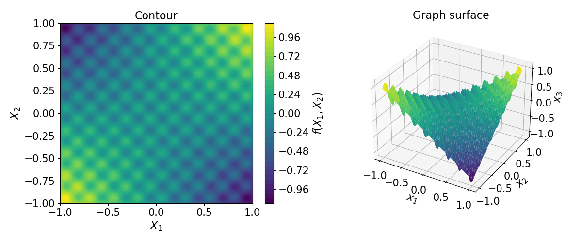
An interesting application of elliptic homogenization is heat conduction on surfaces with multiscale curvature. If the problem is formulated in terms of a parameterization of the surface, we must homogenize the “Laplace-Beltrami” operator, which is the generalization of the Laplacian to thin, curved surfaces. Multiscale Laplace-Beltrami problems have received little attention in the literature [3, 1, 2], though they may be used for modeling heat conduction on wrinkled and/or rough surfaces. To motivate this problem, consider a graph surface given by:

$$\mathbf{x}(\mathbf{X};\eta)=\begin{bmatrix}X_{1}\\ X_{2}\\ f(X_{1},X_{2};\eta)\end{bmatrix}.$$ (14)

An example of this is shown in Figure 8, where $f(X_{1},X_{2};\eta)=X_{1}X_{2}+\eta\sin(2\pi X_{1}/\eta)\sin(2\pi X_{2}/\eta)$ for $\eta=0.25$. This is a surface parameterized by the two coordinates $X_{1}$ and $X_{2}$, and $\eta$ again controls the frequency of oscillation. The metric tensor and its determinant are given by

$$g_{ij}=\frac{\partial\mathbf{x}}{\partial X_{i}}\cdot\frac{\partial\mathbf{x}}{\partial X_{j}},\quad|\mathbf{g}|=\det\mathbf{g}.$$ (15)

Suppose that we have a temperature field $U(\mathbf{X})$ defined on a thin surface parameterized by $\mathbf{x}(\mathbf{X})$. Steady-state temperature distributions on the thin surface have zero Laplacian when the normal components of the gradient and divergence are projected out. To avoid solving the projected Laplace problem in three spatial dimensions, we can compute this surface Laplacian quantity in terms of the parameters $\mathbf{X}$. As shown in Appendix B, this gives rise to the Laplace-Beltrami operator $\Delta_{M}$, which governs steady-state temperature distributions on the surface:

$$\Delta_{M}U:=\frac{1}{\sqrt{|\mathbf{g}|}}\frac{\partial}{\partial X_{i}}\quantity(\sqrt{|\mathbf{g}|}g^{-1}_{ij}\frac{\partial U}{\partial X_{j}}),\quad\Delta_{M}U=0.$$ (16)

Here, we assume that the conductivity of the material is unity, i.e., $\kappa=1$. In the absence of source terms, we note that the factor $1/\sqrt{|\mathbf{g}|}$ can be multiplied out of Eq. (16). In this case, The Laplace-Beltrami problem is simply an elliptic partial differential equation with coefficient field $\sqrt{|\mathbf{g}|}\mathbf{g}^{-1}$. If the surface parameterization varies periodically with $\eta$, so will the metric tensor:

$$\frac{\partial}{\partial X_{i}}\quantity(\sqrt{|\mathbf{g}|(\mathbf{X};\eta)}g^{-1}_{ij}(\mathbf{X};\eta)\frac{\partial U}{\partial X_{j}})=0.$$

It is thus natural to seek to homogenize the effective coefficient field arising from the pull-back of the Laplacian to the parametric domain. This effectively “averages out” the effect of curvature on the heat conduction problem, changing the effective conductivity based on the modified distances that heat needs to traverse along the surface. Except for the fact that the Laplace-Beltrami coefficient field is anisotropic, the derivation of the homogenized tensor follows the derivation in the previous section and Appendix A. Note that when the metric tensor changes with both $\mathbf{X}$ and $\mathbf{X}/\eta$, the cell problem needs to be solved at every point in the macroscopic domain $\Omega_{X}$. In principle, this is not a problem, but in practice it can incur a high computational cost.

To illustrate homogenization of Laplace-Beltrami for cell problems which vary at each point in the domain, we consider a one-dimensional graph surface. The parameterized curve is given by

$$\mathbf{x}(X)=\begin{bmatrix}X\\ \sin(\pi X)+\eta\sin(2\pi X/\eta)\end{bmatrix},\quad X\in[0,1].$$

The metric is thus scalar:

$$g=\frac{\partial\mathbf{x}}{\partial X}\cdot\frac{\partial\mathbf{x}}{\partial X}=1+\pi^{2}\Big(\cos^{2}(\pi X)+4\cos(\pi X)\cos(2\pi X/\eta)+4\cos^{2}(2\pi X/\eta)\Big).$$

In one dimension, the Laplace-Beltrami problem we consider is

$$\frac{\partial}{\partial X}\quantity(\frac{1}{\sqrt{g(X;\eta)}}\frac{\partial U}{\partial X})=0,\quad U(0)=0,\quad\frac{1}{\sqrt{g(1;\eta)}}\frac{\partial U}{\partial X}(1)=h.$$

Identifying $g^{-1/2}\leftrightarrow\kappa$, we define the variable $Y=X/\eta$ to build cell problems. In particular, we define the cell corresponding to point $X$ as given by $\kappa(X,Y)$, where $X$ indexes the slow variation and $Y$ indexes the fast variation. Using Eq. (5), the homogenized material property is

$$\hat{\kappa}(X)=\quantity(\int_{0}^{1}\frac{d\xi}{\kappa(X,\xi)})^{-1},$$

where $Y\in[0,1]$ gives a single period of the microstructural fluctuation. We associate a chunk of microstructure given by one period of the fluctuation to each point $X$, where the slow variation in the material property sets the average conductivity in the cell at the point. The introduction of slow and fast variables is simply a convenient way to construct cell problems when the material property varies on both scales. Using the homogenized material property, which now has only macroscopic dependence, we solve the following homogenized boundary value problem:

$$\frac{\partial}{\partial X}\quantity(\hat{\kappa}(X)\frac{\partial U}{\partial X})=0,\quad U(0)=0,\quad\hat{\kappa}(1)\frac{\partial U}{\partial X}(1)=h.$$

Taking $h=10$, Figure 9 shows the exact and homogenized solutions for three settings of $\eta$. Once again, we see that the scale separation assumption need not be strictly satisfied for the homogenized solution to be accurate.

Figure 9: At three different values of $\eta$, we show the graph surface on which heat conduction takes place (left column), the multiscale material property induced by the Laplace-Beltrami equation (center column), and a comparison of the exact and homogenized solutions (right column). With fluctuations in the temperature that die out as $\eta\rightarrow 0$, the Laplace-Beltrami equation behaves like any other elliptic operator. This means that it can be homogenized using the same techniques developed above.

4 Conclusion

We have sketched a way of thinking about elliptic homogenization that does not require perturbation theory or a strong notion of scale separation. In the context of heat transfer, the homogenized material property is obtained simply by removing a chunk, or cell, of microstructure, imposing uniform temperature gradients, and computing the resulting flux in different coordinate directions. We saw that periodic boundary conditions on the corrector field in the cell were one way to ensure that the flux through the cell was well-defined, meaning that the total flux through cross-sections did not depend on the position of the cross-section. We then discussed the Laplace-Beltrami operator, which models heat conduction on thin curved surfaces. This gives rise to an elliptic boundary value problem, which has seen minimal treatment in the homogenization literature. The multiscale Laplace-Beltrami operator has a number of interesting applications, chief among which is heat conduction on wrinkled surfaces. By homogenizing the coefficient field arising from pulling back to the surface parameters, it is possible to build effective thermal properties that account for the modified distances heat travels on the surface. Future notes may focus on intuitive approaches to non-linear homogenization, and future work on applying the multiscale Laplace-Beltrami problem to wrinkled materials from real-world applications.

Appendix A Elliptic homogenization with perturbation theory

We derive the effective conductivity tensor using the standard approach based on perturbation theory. The governing equation is

$$\frac{\partial}{\partial X_{i}}\quantity(\kappa(\mathbf{X};\eta)\frac{\partial U}{\partial X_{i}})=0,$$

where $\eta\ll 1$ is a scale parameter that controls the frequency of the periodic oscillations of the material. We introduce a “fast coordinate” $\mathbf{Y}=\mathbf{X}/\eta$, which is taken to be independent of $\mathbf{X}$. The conductivity is taken to have both slow and fast fluctuations. Following the standard approach to periodic homogenization, we write the multiscale Laplace problem as

$$\frac{\partial}{\partial X^{\eta}_{i}}\quantity(\kappa(\mathbf{X},\mathbf{Y})\frac{\partial U^{\eta}}{\partial X_{i}^{\eta}})=0,\quad\frac{\partial}{\partial X^{\eta}_{i}}=\frac{\partial}{\partial X_{i}}+\frac{1}{\eta}\frac{\partial}{\partial Y_{i}},\quad U^{\eta}(\mathbf{X},\mathbf{Y})=U^{0}(\mathbf{X})+\eta U^{1}(\mathbf{X},\mathbf{Y}),$$

Plugging in the definition of the multiscale temperature, the definition of the multiscale derivative, and taking note of the dependencies of each variable in the above expression, we can expand the multiscale Laplace problem:

$$\frac{\partial}{\partial X_{i}}\quantity(\kappa\frac{\partial U^{0}}{\partial X_{i}})+\frac{1}{\eta}\frac{\partial}{\partial Y_{i}}\quantity(\kappa\frac{\partial U^{0}}{\partial X_{i}})+\eta\frac{\partial}{\partial X_{i}}\quantity(\kappa\frac{\partial U^{1}}{\partial X_{i}})+\frac{\partial}{\partial Y_{i}}\quantity(\kappa\frac{\partial U^{1}}{\partial X_{i}})$$

$$+\frac{\partial}{\partial X_{i}}\quantity(\kappa\frac{\partial U^{1}}{\partial Y_{i}})+\frac{1}{\eta}\frac{\partial}{\partial Y_{i}}\quantity(\kappa\frac{\partial U^{1}}{\partial Y_{i}}).$$

The terms multiplying $\eta^{-1}$ provide the cell problem:

$$\frac{\partial}{\partial Y_{i}}\quantity(\kappa\frac{\partial U^{1}}{\partial Y_{i}})=-\frac{\partial\kappa}{\partial Y_{i}}\frac{\partial U^{0}}{\partial X_{i}}.$$

Now, by linearity, we define a solution to this problem as $U^{1}(\mathbf{X},\mathbf{Y})=\chi_{j}(\mathbf{X},\mathbf{Y})\frac{\partial U^{0}}{\partial X_{j}}(\mathbf{X})$, where $\chi_{j}$ is the solution of the above equation for $\partial U^{0}/\partial X_{j}=\mathbf{e}_{j}$ and has periodic boundary conditions. The so-called “macroscale” equation is obtained by looking at terms of order $\eta^{0}$:

$$\frac{\partial}{\partial X_{i}}\quantity(\kappa\frac{\partial U^{0}}{\partial X_{i}})+\frac{\partial}{\partial Y_{i}}\quantity(\kappa\frac{\partial U^{1}}{\partial X_{i}})+\frac{\partial}{\partial X_{i}}\quantity(\kappa\frac{\partial U^{1}}{\partial Y_{i}})=0.$$

We use the result of the cell problem to write the microscale solution in terms of the macroscale solution:

$$\frac{\partial}{\partial X_{i}}\quantity(\kappa\frac{\partial U^{0}}{\partial X_{i}})+\frac{\partial}{\partial Y_{i}}\quantity(\kappa\chi_{k}\frac{\partial^{2}U^{0}}{\partial X_{k}\partial X_{i}})+\frac{\partial}{\partial X_{i}}\quantity(\kappa\frac{\partial\chi_{k}}{\partial Y_{i}}\frac{\partial U^{0}}{\partial X_{k}})=0.$$

Now, note that this equation cannot be satisfied pointwise in $\mathbf{Y}$, as the unknown solution $U^{0}(\mathbf{X})$ is purely macroscopic, yet $\kappa$ and $\boldsymbol{\chi}$ have slow and fast components. This equation can only be satisfied in an average sense:

$$\int_{\Omega_{Y}}\quantity[\frac{\partial}{\partial X_{i}}\quantity(\kappa\frac{\partial U^{0}}{\partial X_{i}})+\frac{\partial}{\partial Y_{i}}\quantity(\kappa\chi_{k}\frac{\partial^{2}U^{0}}{\partial X_{k}\partial X_{i}})+\frac{\partial}{\partial X_{i}}\quantity(\kappa\frac{\partial\chi_{k}}{\partial Y_{i}}\frac{\partial U^{0}}{\partial X_{k}})]d\Omega=0.$$

We now use the fact that the microscale corrector $\boldsymbol{\chi}$ is periodic. The integral of the divergence of a periodic quantity is zero, thus we can cancel a term and refactor to obtain the homogenized governing equation:

$$\frac{\partial}{\partial X_{j}}\quantity[\int_{\Omega_{Y}}\kappa\quantity(\delta_{j\ell}+\frac{\partial\chi_{\ell}}{\partial Y_{j}})d\Omega\frac{\partial U^{0}}{\partial X_{\ell}}]=0.$$

The homogenized coefficient tensor is thus

$$\boldsymbol{\hat{\kappa}}(\mathbf{X})=\int_{\Omega_{Y}}\kappa(\mathbf{X},\mathbf{Y})\quantity(\delta_{j\ell}+\frac{\partial\chi_{\ell}(\mathbf{X},\mathbf{Y})}{\partial Y_{j}})d\Omega.$$

Appendix B Derivation of the Laplace-Beltrami operator

Figure 10: Transformation of an area element between the intrinsic and extrinsic descriptions of the surface. We use these relationships to derive the Laplace-Beltrami operator.

Here, we derive the Laplace-Beltrami operator on a parameterized surface $\mathbf{x}(\mathbf{X})$ from definitions of the divergence and gradient. We refer to descriptions of the surface in terms of the parameters $\mathbf{X}\in\mathbb{R}^{2}$ as intrinsic, and descriptions of the surface in $\mathbb{R}^{3}$ as extrinsic. We begin by computing the intrinsic divergence $\nabla_{M}\cdot()$ of a vector field $\mathbf{V}(\mathbf{X})$ defined in terms of the tangent basis $\mathbf{x}_{1}=\frac{\partial\mathbf{x}}{\partial X_{1}}$ and $\mathbf{x}_{2}=\frac{\partial\mathbf{x}}{\partial X_{2}}$, i.e., $\mathbf{V}=V_{i}\mathbf{x}_{i}$. The two-dimensional divergence is defined as the net outflow per area at a point. Thus, to compute the divergence operator, we find the flux through the sides of an area element on the surface. For a small area $\Delta X_{1}\Delta X_{2}$ in the intrinsic coordinate system, the corresponding area element on the surface is $\sqrt{|\mathbf{g}|}\Delta X_{1}\Delta X_{2}$. The side lengths transform with $\lVert\mathbf{x}_{i}\rVert^{2}\Delta X_{i}^{2}=g_{ii}\Delta X_{i}^{2}$, where the metric is evaluated at the center point of the side in the intrinsic coordinates. We also evaluate the vector field $\mathbf{V}(\mathbf{X})$ at the centers of the sides in the intrinsic coordinates, and approximate it as constant over the sides in computing the flux. In computing the flux, we need to extract the component of the vector field normal to the side. To this end, we introduce the “dual basis” $\mathbf{x}^{i}$, which is defined as

$$\mathbf{x}^{i}\cdot\mathbf{x}_{j}=\mathbf{g}^{-1}_{ik}\mathbf{x}_{k}\cdot\mathbf{x}_{j}=\delta_{ij}.$$

Note that this implies the dual basis is orthogonal to the tangent vectors which define the sides of the area element on the surface. We can show that $\mathbf{x}^{i}\cdot\mathbf{x}^{j}=\mathbf{g}^{-1}_{ij}$, meaning that the dual basis is neither normalized nor orthogonal. A useful property of the dual basis is that

$$\mathbf{V}\cdot\mathbf{x}^{i}=\sum_{j}V_{j}\mathbf{x}_{j}\cdot\mathbf{x}^{i}=V_{i},$$

meaning that $V_{i}$ gives the component of $\mathbf{V}$ normal to the side aligned with the $X_{i}$ direction. With these results, we can compute the fluxes through the four sides as follows:

$$\text{top}=V_{2}(X_{1},X_{2}+\Delta X_{2}/2)\Delta X_{1}\sqrt{g_{11}(X_{1},X_{2}+\Delta X_{2}/2)}/\sqrt{g^{-1}_{22}(X_{1},X_{2}+\Delta X_{2}/2)},$$

$$\text{bottom}=-V_{2}(X_{1},X_{2}-\Delta X_{2}/2)\Delta X_{1}\sqrt{g_{11}(X_{1},X_{2}-\Delta X_{2}/2)}/\sqrt{g^{-1}_{22}(X_{1},X_{2}-\Delta X_{2}/2)},$$

$$\text{right}=V_{1}(X_{1}+\Delta X_{1}/2,X_{2})\Delta X_{2}\sqrt{g_{22}(X_{1}+\Delta X_{1}/2,X_{2})}/\sqrt{g^{-1}_{11}(X_{1}+\Delta X_{1}/2,X_{2})},$$

$$\text{left}=-V_{1}(X_{1}-\Delta X_{1}/2,X_{2})\Delta X_{2}\sqrt{g_{22}(X_{1}-\Delta X_{1}/2,X_{2})}/\sqrt{g^{-1}_{11}(X_{1}-\Delta X_{1}/2,X_{2})}.$$

In the case of $2\times 2$ matrices, we have that $\sqrt{g_{11}}/\sqrt{g^{-1}_{22}}=\sqrt{g_{22}}/\sqrt{g^{-1}_{11}}=\sqrt{|\mathbf{g}|}$. With this, we can write

$$\nabla_{M}\cdot\mathbf{V}=\lim_{\text{area}\rightarrow 0}\frac{\text{flow out}}{\text{area}}=\lim_{\Delta X_{1}\Delta X_{2}\rightarrow 0}\frac{1}{\sqrt{|\mathbf{g}|}\Delta X_{1}\Delta X_{2}}(\text{top}+\text{bottom}+\text{right}+\text{left})=\frac{1}{\sqrt{|\mathbf{g}|}}\frac{\partial}{\partial X_{i}}(\sqrt{|\mathbf{g}|}V_{i}).$$

With the divergence defined, we now use it to compute the Laplacian. The intrinsic Laplacian is defined as $\Delta_{M}U(\mathbf{X})=\nabla_{M}\cdot\nabla_{M}U(\mathbf{X})$. Thus, we need to determine how to compute the gradient of a scalar field with respect to intrinsic coordinates. To this, we note that the differential of a scalar field is a coordinate-independent quantity. This allows us to find a relationship between $\partial U/\partial X_{i}$ and the extrinsic representation of the gradient in terms of the tangent basis:

$$dU=\frac{\partial U}{\partial X_{i}}a_{i}=V_{j}\mathbf{x}_{j}\cdot a_{i}\mathbf{x}_{i}\implies V_{j}=g^{-1}_{jk}\frac{\partial U}{\partial X_{k}},$$

where the coefficients $a_{i}$ define an arbitrary direction in which to compute the differential $dU$ and the $V_{j}$ are the coordinates of the gradient vector in terms of the tangent basis. Combining this result with the expression for the divergence, we obtain the Laplace-Beltrami operator as

$$\Delta_{M}U=\frac{1}{\sqrt{|\mathbf{g}|}}\frac{\partial}{\partial X_{i}}\quantity(\sqrt{|\mathbf{g}|}g^{-1}_{ij}\frac{\partial U}{\partial X_{j}}).$$

References

- [1] M. Amar, D. Andreucci, R. Gianni, and C. Timofte. Concentration and homogenization in electrical conduction in heterogeneous media involving the Laplace–Beltrami operator. Calculus of Variations and Partial Differential Equations, 59(3):99, May 2020.
- [2] Micol Amar and Roberto Gianni. Error estimate for a homogenization problem involving the Laplace-Beltrami operator, May 2017.
- [3] María Anguiano. Homogenization of parabolic problems with dynamical boundary conditions of reactive-diffusive type in perforated media, December 2019.
- [4] O. A. Bauchau and J. I. Craig. Structural Analysis: With Applications to Aerospace Structures. Springer Science & Business Media, August 2009. Google-Books-ID: GYRX8ZYVNYQC.
- [5] Alain Bensoussan, Jacques-Louis Lions, George Papanicolaou, and T. K. Caughey. Asymptotic Analysis of Periodic Structures. In Journal of Applied Mechanics, volume 46, pages 477–477, June 1979.
- [6] G. A. Francfort and F. Murat. Homogenization and optimal bounds in linear elasticity. Archive for Rational Mechanics and Analysis, 94(4):307–334, December 1986.
- [7] M. Kaviany. Fluid Mechanics. In M. Kaviany, editor, Principles of Heat Transfer in Porous Media, pages 15–113. Springer US, New York, NY, 1991.
- [8] Vinh Tung Le and Nam Seo Goo. Improved Metallic Thermal Protection Systems for Reentry Vehicles: Thermomechanical and Impact Considerations. Journal of Spacecraft and Rockets, 62(2):433–451, March 2025.
- [9] James Davis A. Senig and John F. Maddox. An Investigation Into the Effective Gaseous Thermal Conductivity of Fibrous Insulation Materials. In AIAA AVIATION FORUM AND ASCEND 2024. American Institute of Aeronautics and Astronautics, 2025. _eprint: https://arc.aiaa.org/doi/pdf/10.2514/6.2024-4030.
- [10] Takahiro Yamaguchi and Tsukasa Mizutani. A Physics-Informed Neural Network for the Nonlinear Damage Identification in a Reinforced Concrete Bridge Pier Using Seismic Responses. Structural Control and Health Monitoring, 2024(1):5532909, 2024. _eprint: https://onlinelibrary.wiley.com/doi/pdf/10.1155/2024/5532909.
- [11] I. Özdemir, W. a. M. Brekelmans, and M. G. D. Geers. Computational homogenization for heat conduction in heterogeneous solids. International Journal for Numerical Methods in Engineering, 73(2):185–204, 2008. _eprint: https://onlinelibrary.wiley.com/doi/pdf/10.1002/nme.2068.