Event-Driven Video Generation

Abstract

State-of-the-art text-to-video models often look realistic frame-by-frame yet fail on simple interactions: motion starts before contact, actions are not realized, objects drift after placement, and support relations break. We argue this stems from frame-first denoising, which updates latent state everywhere at every step without an explicit notion of when and where an interaction is active. We introduce Event-Driven Video Generation (EVD), a minimal DiT-compatible framework that makes sampling event-grounded: a lightweight event head predicts token-aligned event activity, event-grounded losses couple activity to state change during training, and event-gated sampling (with hysteresis and early-step scheduling) suppresses spurious updates while concentrating updates during interactions. On EVD-Bench, EVD consistently improves human preference and VBench dynamics, substantially reducing failure modes in state persistence, spatial accuracy, support relations, and contact stability without sacrificing appearance. These results indicate that explicit event grounding is a practical abstraction for reducing interaction hallucinations in video generation.

1 Introduction

Recent video foundation models have advanced rapidly in realism, resolution, and duration, pushing text-to-video toward general-purpose visual simulation at scale. Space–time diffusion architectures can synthesize temporally coherent clips in a single pass (e.g., Lumiere [1]), while large diffusion-transformer systems scale training recipes, latent representations, and context lengths to high-fidelity long videos (e.g., Movie Gen [22], Step-Video-T2V [17]). In parallel, open and semi-open efforts narrow the gap through systematic data curation and infrastructure (e.g., HunyuanVideo [12], Open-Sora [32], Wan [25]) and faster/efficient sampling paradigms (e.g., Pyramidal Flow Matching [11], T2V-Turbo/T2V-Turbo-v2 [13, 14]), enabling increasingly compelling generations.

2 Motivation

Figure 2: Failure taxonomy of DiT-30B under simple physical interactions. Examples of systematic breakdowns in DiT-30B generations: (a) state persistence, e.g., post-interaction dynamics (the chair continues moving after the pulling action has ceased); (b) spatial accuracy, e.g., object placement (the cube fails to align with the intended platform); (c) support relations, e.g., event realization (the book appears stacked without a visible stacking action); and (d) contact stability, e.g., causal initiation (the plate begins moving before any hand–object contact occurs).

Despite these gains, interaction-heavy prompts still expose a persistent bottleneck: videos can look locally smooth yet violate causal structure—effects before causes, missing contacts, and unstable postconditions—which undermines physical credibility even in simple everyday scenes. This weakness is reflected in contemporary evaluation efforts that decompose “video quality” into motion/physics/consistency axes and stress that superficial fidelity does not imply intrinsically realistic dynamics (VBench [9], VBench++ [10], VBench-2.0 [30]). Empirically, recent large models can score well on appearance while still failing on interaction grounding, motivating methods that explicitly target motion and dynamics rather than relying on scale alone [23].

Existing SOTA work improves dynamics via better architectures and training/inference recipes (e.g., CogVideoX [27], Open-Sora STDiT [32], HunyuanVideo [12], Step-Video-T2V [17]), and via motion-focused objectives and inference-time steering that address the appearance–motion imbalance (VideoJAM [4]). However, these approaches largely remain “frame-first”: the sampler updates the latent state everywhere at every step, allowing spurious changes that are locally plausible but globally ungrounded in discrete interaction events. As illustrated in Fig. 2, strong DiT backbones can produce visually plausible frames while violating event causality—e.g., pre-contact motion, missing interaction realization, and post-event drift—which we summarize into four recurring failure categories (State Persistence, Spatial Accuracy, Support Relations, Contact Stability). In other words, interaction realism requires an internal notion of event activity (whether an interaction is happening here/now) that can gate where/when the latent is allowed to change, so contact initiation, constrained motion, and settling emerge as event-conditioned state transitions rather than incidental artifacts of denoising.

3 Contributions

We propose Event-Driven Video Generation (EVD), a minimal DiT-compatible mechanism that makes latent evolution explicitly event-grounded. EVD (i) attaches a lightweight event head to DiT token features to predict a token-aligned event activity map, (ii) trains with event-grounded losses that suppress updates when no event is active and stabilize updates during interactions, and (iii) modifies sampling by gating the solver direction field with a hysteresis-and-schedule rule that concentrates updates early when events form and attenuates spurious late-step drift. The result is a backbone-agnostic recipe that composes naturally with modern DiT video systems [22, 17, 27, 32] and improves interaction realism without changing the solver family or decoding stack; remaining limitations arise when event signals are weak/ambiguous at operating resolution (e.g., small/occluded contacts or cluttered multi-object scenes), suggesting future object-centric or contact-aware event cues.

4 EVD

This section presents Event-Driven Video Generation (EVD), a minimal modification of a pretrained video DiT backbone that enforces event-grounded state transitions. We first set up notation and the latent-video backbone interface (Sec. 4.1.1), then introduce the core event-gated update rule and the event head used to predict token-aligned event activity (Sec. 4.2.1). Next, we specify the event gate (soft activation with hysteresis) and the resulting gated direction field (Sec. 4.2.3). We then derive the training objective—base Flow Matching plus event realization, consistency, ordering, and time-weighting terms (Sec. 4.3)— and finally describe event-driven inference with scheduled gating under CFG (Sec. 4.4). For full reproducibility, Algorithms 2 and 1 provide self-contained training and sampling pseudocode, and Sec. 4.5 lists the default hyperparameters used in our experiments.

4.1 Method: Event-Driven Video Generation (EVD)

4.1.1 Latent video representation and notation

We consider text-conditioned video generation. A video clip is denoted by $x\in\mathbb{R}^{T\times H\times W\times 3}$ with $T$ frames. Following standard practice in large-scale video diffusion/flow models, we generate in a compressed latent space using a temporal video autoencoder. Let $E(\cdot)$ and $D(\cdot)$ denote the encoder and decoder, and define the latent video

$$z=E(x),\qquad x\approx D(z),$$ (1)

where $z\in\mathbb{R}^{T^{\prime}\times H^{\prime}\times W^{\prime}\times C}$ has reduced spatiotemporal resolution.

Let $y$ denote the text prompt, encoded by a frozen text encoder into a sequence of embeddings. We denote the DiT backbone by $u_{\theta}(\cdot)$, parameterized by $\theta$, which operates on noised latents and conditions on $(y,t)$, where $t\in[0,1]$ is the continuous diffusion/flow time.

Noise model and training target.

We use a continuous-time Flow Matching formulation in latent space [15, 20, 18]. Given a clean latent $z_{1}$ and noise $z_{0}\sim\mathcal{N}(0,I)$, we sample $t\sim\mathcal{U}[0,1]$ and form the interpolated latent

$$z_{t}=t\,z_{1}+(1-t)\,z_{0},$$ (2)

with velocity target

$$v_{t}=\frac{dz_{t}}{dt}=z_{1}-z_{0}.$$ (3)

The backbone predicts $\widehat{v}_{t}=u_{\theta}(z_{t},y,t)$. EVD preserves this backbone interface and modifies how the model represents and applies event-driven state changes in subsequent subsections.

4.1.2 DiT backbone and conditioning interface

EVD is built on a pretrained video Diffusion Transformer (DiT) operating in latent space. Given $z_{t}\in\mathbb{R}^{T^{\prime}\times H^{\prime}\times W^{\prime}\times C}$, we patchify $z_{t}$ into spatiotemporal tokens and map them to the model width $d$, yielding a token sequence $\mathbf{s}_{t}\in\mathbb{R}^{N\times d}$, where $N$ is the number of spatiotemporal patches. The DiT applies $L$ transformer blocks with spatiotemporal self-attention and text cross-attention, producing final features $\mathbf{s}_{t}^{(L)}$.

The DiT backbone outputs a prediction of the Flow Matching velocity (Eq. (3)):

$$\widehat{v}_{t}\;=\;u_{\theta}(z_{t},y,t).$$ (4)

We do not modify the backbone architecture or its tokenization; EVD introduces an additional lightweight event pathway that predicts event activity aligned with the same token grid and uses it to gate updates during training and sampling (Secs. 4.2–4.4).

Sampling interface.

Sampling evolves a latent trajectory $\{z_{t_{k}}\}_{k=0}^{K}$ along a monotone time grid $0=t_{0}<\cdots<t_{K}=1$. At each step, the sampler queries the backbone to obtain a direction field and updates $z_{t_{k}}$ using a solver step (Euler/Heun/DPM-style [31]). EVD is compatible with any such solver because it only changes the direction field passed to the solver.

4.1.3 Classifier-free guidance (CFG)

We use classifier-free guidance (CFG) to improve prompt adherence. At each sampling step $t_{k}$, we evaluate the backbone with the prompt $y$ and with a null prompt $\varnothing$, and form the guided direction field

$$\widehat{v}^{\mathrm{cfg}}(z_{t_{k}},y,t_{k})\;=\;(1+w_{\mathrm{cfg}})\,u_{\theta}(z_{t_{k}},y,t_{k})\;-\;w_{\mathrm{cfg}}\,u_{\theta}(z_{t_{k}},\varnothing,t_{k}),$$ (5)

where $w_{\mathrm{cfg}}\geq 0$ is the guidance scale. EVD applies event gating after forming $\widehat{v}^{\mathrm{cfg}}$, so prompt adherence is preserved while spurious, event-inconsistent dynamics are suppressed (Sec. 4.4).

4.1.4 Why frame-first generation fails on interactions

Although modern video generators can produce locally smooth motion [1, 22, 12, 32, 17, 4, 8, 26], they often violate basic causal structure in simple interactions: effects appear without causes (e.g., objects move before contact), causes occur without coherent effects (e.g., an interaction is implied but the state does not respond), and post-interaction states drift instead of settling. These errors are particularly salient in prompts involving contact, support, constrained mechanisms, or material transfer, and they map directly to the four failure categories used in our analysis: State Persistence, Spatial Accuracy, Support Relations, and Contact Stability.

4.2 Event-Driven Video Generation

4.2.1 Core idea: event-gated state updates

EVD models a video as persistent latent state punctuated by discrete interaction events. At diffusion/flow time $t$, we introduce an event representation $e_{t}$ aligned with the DiT token grid, and derive from it an event gate $g_{\psi}(e_{t},t)\in[0,1]^{N}$ (token-wise, broadcast across channels). The gate modulates the backbone direction field so that state updates occur only when justified by an active interaction:

$$\Delta z_{t}\;=\;\mathrm{UnTok}\!\Big(g_{\psi}(e_{t},t)\odot\mathrm{Tok}\big(u_{\theta}(z_{t},y,t)\big)\Big).$$ (6)

When the event signal indicates “no interaction” (gate near zero), the update is suppressed and the state remains stable; when an event is active (gate near one), the update proceeds normally. This single mechanism targets both common degeneracies: missing events (state changes without a visible interaction) and ghost events (an implied interaction without a coherent state change).

In the remainder of this section, we specify (i) how $e_{t}$ and $g_{\psi}$ are instantiated, (ii) the event-grounded training objective, and (iii) the event-driven sampling procedure with CFG.

4.2.2 Event representation and event head

EVD uses a token-aligned event field to localize interactions in space and time. Let $\mathbf{s}_{t}^{(L)}\in\mathbb{R}^{N\times d}$ be the final DiT token features at time $t$. We attach a lightweight event head $\pi_{\psi}$ that predicts an event field

$$\hat{e}_{t}\;=\;\pi_{\psi}(\mathbf{s}_{t}^{(L)},t)\;\in\;\mathbb{R}^{N\times C_{e}},$$ (7)

with a small channel budget $C_{e}$ (we use $C_{e}=1$ in the main method). The first channel is interpreted as an event activity logit, and we obtain a token-wise activity probability via

$$\hat{a}_{t}\;=\;\sigma(\hat{e}_{t}^{(1)})\;\in\;[0,1]^{N},$$ (8)

where $\sigma(\cdot)$ is the sigmoid and $\hat{e}_{t}^{(1)}$ denotes the activity channel.

Zero-impact initialization.

To preserve pretrained DiT behavior at the start of fine-tuning, we initialize $\pi_{\psi}$ to near-zero output so that $\hat{a}_{t}\approx 0$ initially, and the model reduces to the base backbone before learning event structure.

Spatial smoothing.

Event activity can be spatially fragmented due to noise. We apply a lightweight smoothing operator $\mathcal{S}$ over the spatial patch grid (per frame) and use $\tilde{a}_{t}=\mathcal{S}(\hat{a}_{t})$ in all gating computations. In our main setting, $\mathcal{S}$ is a $3\times 3$ average filter.

4.2.3 Event gate: soft activation with hysteresis

We convert the smoothed activity $\tilde{a}_{t}\in[0,1]^{N}$ into a stable, token-wise gate $g_{t}\in[0,1]^{N}$ that controls whether each token is allowed to update. EVD uses soft activation to avoid brittle thresholding and hysteresis to prevent flickering event boundaries.

Soft activation.

We first form a soft gate centered between the on/off thresholds:

$$\bar{g}_{t}\;=\;\sigma\!\Big(\beta\big(\tilde{a}_{t}-\tfrac{\tau_{\mathrm{on}}+\tau_{\mathrm{off}}}{2}\big)\Big),$$ (9)

where $\beta>0$ controls sharpness and $\tau_{\mathrm{on}}>\tau_{\mathrm{off}}$ define the hysteresis band.

Hysteresis update.

We maintain a binary state gate $g_{t}^{\mathrm{bin}}\in\{0,1\}^{N}$ with token-wise update:

$$g^{\mathrm{bin}}_{t,i}\;=\;\begin{cases}1,&\tilde{a}_{t,i}\geq\tau_{\mathrm{on}},\\ 0,&\tilde{a}_{t,i}\leq\tau_{\mathrm{off}},\\ g^{\mathrm{bin}}_{t^{-},i},&\text{otherwise},\end{cases}$$ (10)

where $t^{-}$ denotes the previous sampling step (or previous iteration in the discretized schedule) and $i$ indexes tokens. Finally, we combine soft and hysteresis gates to obtain the effective gate used for modulation:

$$g_{t}\;=\;\bar{g}_{t}\odot g_{t}^{\mathrm{bin}},$$ (11)

Here $g_{t}^{\mathrm{bin}}$ provides stable on/off event activation (prevents flicker), while $\bar{g}_{t}$ smoothly scales update magnitude within active regions; scheduled gating is applied afterward during sampling (Sec. 4.4.1).

In practice this reduces to using the hysteresis state for stability while retaining smooth transitions through $\bar{g}_{t}$. (Algorithm 1 provides the exact implementation used in our experiments.)

Algorithm 1 Event-Driven Sampling (EVD) with CFG

1: Inputs: prompt $y$; null prompt $\varnothing$; time grid $\{t_{k}\}_{k=0}^{K}$; DiT backbone $u_{\theta}$; event head $\pi_{\psi}$; decoder $D$; CFG scale $w_{\mathrm{cfg}}$; gate sharpness $\beta$; hysteresis thresholds $(\tau_{\mathrm{on}},\tau_{\mathrm{off}})$; anneal cutoff $t^{\star}$; spatial smoothing operator $\mathcal{S}$.

2: Operators: $\mathrm{Tok}/\mathrm{UnTok}$ (patchify/unpatchify); $\sigma(\cdot)$ sigmoid; $\odot$ elementwise product.

3: Init: sample latent $z_{t_{0}}\sim\mathcal{N}(0,I)$; initialize gate state $g_{-1}\leftarrow\mathbf{0}$.

4: for $k=0,\dots,K-1$ do

5:  (1) CFG direction field.

6:    $\widehat{\tau}^{\mathrm{cond}}\leftarrow u_{\theta}(z_{t_{k}},y,t_{k})$,  $\widehat{\tau}^{\mathrm{uncond}}\leftarrow u_{\theta}(z_{t_{k}},\varnothing,t_{k})$

7:    $\widehat{\tau}^{\mathrm{cfg}}\leftarrow(1+w_{\mathrm{cfg}})\widehat{\tau}^{\mathrm{cond}}-w_{\mathrm{cfg}}\,\widehat{\tau}^{\mathrm{uncond}}$

8:  (2) Predict event activity (token-aligned).

9:    $\hat{e}_{k}\leftarrow\pi_{\psi}(\mathbf{s}_{t_{k}}^{(L)},t_{k})$

10:    $\hat{a}_{k}\leftarrow\sigma(\hat{e}_{k}^{(1)})\in[0,1]^{N}$ (activity channel)

11:  (3) Smooth activity and compute a soft gate.

12:    $\tilde{a}_{k}\leftarrow\mathcal{S}(\hat{a}_{k})$ (if disabled, set $\tilde{a}_{k}=\hat{a}_{k}$)

13:    $\bar{g}_{k}\leftarrow\sigma\!\big(\beta(\tilde{a}_{k}-\tfrac{\tau_{\mathrm{on}}+\tau_{\mathrm{off}}}{2})\big)\in(0,1)^{N}$

14:  (4) Hysteresis (stabilize on/off).

15:    for each token $i\in\{1,\dots,N\}$: (token-wise update)

16:      $g_{k,i}\leftarrow 1$ if $\tilde{a}_{k,i}\geq\tau_{\mathrm{on}}$; $\;\;g_{k,i}\leftarrow 0$ else if $\tilde{a}_{k,i}\leq\tau_{\mathrm{off}}$; $\;\;g_{k,i}\leftarrow g_{k-1,i}$ otherwise.

17:  $g_{k}\leftarrow\bar{g}_{k}\odot g_{k}^{\mathrm{bin}}$

18:  (5) Time scheduling (strong early, anneal late).

19:    $\rho_{k}\leftarrow\begin{cases}1,&t_{k}\leq t^{\star},\\ 1-\dfrac{t_{k}-t^{\star}}{1-t^{\star}},&t_{k}>t^{\star},\end{cases}$

20:    $g_{k}\leftarrow\rho_{k}\,g_{k}+(1-\rho_{k})\mathbf{1}$ ($\mathbf{1}$: all-ones gate)

21:  (6) Apply gating to the CFG field.

22:    $\widetilde{\tau}_{k}\leftarrow\mathrm{UnTok}\!\big(g_{k}\odot\mathrm{Tok}(\widehat{\tau}^{\mathrm{cfg}})\big)$

23:  (7) Solver step (base sampler unchanged).

24:    $z_{t_{k+1}}\leftarrow\mathrm{Step}(z_{t_{k}},\widetilde{\tau}_{k},t_{k},t_{k+1})$

25: end for

26: Decode: $x\leftarrow D(z_{t_{K}})$.   Return: $x$.

4.2.4 Event-gated update field

Given the backbone prediction $\widehat{v}_{t}=u_{\theta}(z_{t},y,t)$ and the event gate $g_{t}\in[0,1]^{N}$, EVD forms an event-gated direction field by modulating the patchified backbone output and unpatchifying back to latent space:

$$\widetilde{v}_{t}\;=\;\mathrm{UnTok}\!\Big(g_{t}\odot\mathrm{Tok}\big(\widehat{v}_{t}\big)\Big).$$ (12)

We then pass $\widetilde{v}_{t}$ to the same solver used by the base model. Because EVD only changes the direction field, it is compatible with any ODE sampler (Euler/Heun/DPM-style) used for DiT video generation.

4.3 Training Objective

EVD preserves the base Flow Matching objective (Eqs. (2)–(3)) and adds event-grounded terms that couple event activity to state evolution. Let $\widehat{v}_{t}=u_{\theta}(z_{t},y,t)$ be the predicted velocity and $\Delta_{t}=\mathrm{Tok}(\widehat{v}_{t})$ its token form.

4.3.1 Base Flow Matching loss

The base loss matches the predicted velocity to the target $v_{t}=z_{1}-z_{0}$:

$$\mathcal{L}_{\mathrm{base}}\;=\;\mathbb{E}_{z_{1},z_{0},t,y}\Big[\big\|u_{\theta}(z_{t},y,t)-(z_{1}-z_{0})\big\|_{2}^{2}\Big].$$ (13)

4.3.2 Event realization loss

To prevent missing events (state changes without an active interaction), we penalize update energy in tokens where the event activity is low:

$$\mathcal{L}_{\mathrm{real}}\;=\;\mathbb{E}\Big[\big\|(1-\tilde{a}_{t})\odot\Delta_{t}\big\|_{2}^{2}\Big],$$ (14)

where $\tilde{a}_{t}$ is the smoothed event activity (Sec. 4.2.2). This term forces the model to either (i) predict an active event where a state change is required, or (ii) suppress the state change when no event is present.

4.3.3 Event consistency loss

To prevent ghost events and reduce jitter during interactions, we enforce that state updates under active events are locally consistent across nearby diffusion/flow times. For each training sample we draw a second time $t^{\prime}=\mathrm{clip}(t+\delta,0,1)$ with $\delta\sim\mathcal{U}[-\Delta,\Delta]$, construct $z_{t^{\prime}}=t^{\prime}z_{1}+(1-t^{\prime})z_{0}$, and compute $\Delta_{t}=\mathrm{Tok}(u_{\theta}(z_{t},y,t))$, $\Delta_{t^{\prime}}=\mathrm{Tok}(u_{\theta}(z_{t^{\prime}},y,t^{\prime}))$, with corresponding activities $\tilde{a}_{t}$ and $\tilde{a}_{t^{\prime}}$. We then minimize the event-masked discrepancy:

$$\mathcal{L}_{\mathrm{cons}}\;=\;\mathbb{E}\Big[\big\|\tilde{a}_{t}\odot\Delta_{t}-\tilde{a}_{t^{\prime}}\odot\Delta_{t^{\prime}}\big\|_{2}^{2}\Big].$$ (15)

Intuitively, once an interaction is active, the model should not oscillate between incompatible update directions across infinitesimally close times; $\mathcal{L}_{\mathrm{cons}}$ encourages stable, directed state evolution during the event.

4.3.4 Ordering and termination loss

EVD additionally enforces a simple causal ordering: motion should not occur before event initiation and should decay after termination. Using the same thresholds that define the hysteresis band ($\tau_{\mathrm{on}}>\tau_{\mathrm{off}}$), we suppress update energy in low-activity regions:

$$\mathcal{L}_{\mathrm{order}}\;=\;\mathbb{E}\Big[\big\|\mathbf{1}[\tilde{a}_{t}<\tau_{\mathrm{on}}]\odot\Delta_{t}\big\|_{2}^{2}+\big\|\mathbf{1}[\tilde{a}_{t}<\tau_{\mathrm{off}}]\odot\Delta_{t}\big\|_{2}^{2}\Big],$$ (16)

where $\mathbf{1}[\cdot]$ is applied token-wise. The first term discourages pre-event motion (improving Contact Stability); the second term suppresses residual updates after the model indicates the event is off (improving State Persistence).

4.3.5 Time-weighted objective

Event grounding matters most at early diffusion/flow times that determine coarse dynamics. We therefore apply a time weight

$$w(t)=\mathbf{1}[t\leq t^{\star}_{\mathrm{loss}}]+\exp\!\big(-\kappa(t-t^{\star}_{\mathrm{loss}})\big)\mathbf{1}[t>t^{\star}_{\mathrm{loss}}],$$ (17)

and optimize the total objective

$$\mathcal{L}\;=\;\mathcal{L}_{\mathrm{base}}+w(t)\Big(\lambda_{\mathrm{real}}\mathcal{L}_{\mathrm{real}}+\lambda_{\mathrm{cons}}\mathcal{L}_{\mathrm{cons}}+\lambda_{\mathrm{order}}\mathcal{L}_{\mathrm{order}}\Big).$$ (18)

Algorithm 2 provides the complete training procedure.

Algorithm 2 Event-Driven Video Generation (EVD): training

1: Inputs: paired data $(x,y)$; video encoder $E$; DiT backbone $u_{\theta}$; event head $\pi_{\psi}$; loss weights $(\lambda_{\mathrm{real}},\lambda_{\mathrm{cons}},\lambda_{\mathrm{order}})$; loss time-weight cutoff $t^{\star}_{\mathrm{loss}}$ and decay $\kappa$; consistency jitter $\Delta$; event-dropout $p_{e}$; hysteresis thresholds $(\tau_{\mathrm{on}},\tau_{\mathrm{off}})$.

2: Operators: $\mathrm{Tok}(\cdot)$ patchify; $\sigma(\cdot)$ sigmoid; $\odot$ elementwise product; $\mathbf{1}[\cdot]$ indicator.

3: Loss time-weight: $w(t)=\mathbf{1}[t\leq t^{\star}_{\mathrm{loss}}]+\exp(-\kappa(t-t^{\star}_{\mathrm{loss}}))\mathbf{1}[t>t^{\star}_{\mathrm{loss}}]$.

4: Train (DiT + event head; event-grounded losses).

5: for each minibatch $(x,y)$ do

6:  Encode: $z_{1}\leftarrow E(x)$; sample $z_{0}\sim\mathcal{N}(0,I)$; sample $t\sim\mathcal{U}[0,1]$.

7:  Flow-matching form: $z_{t}\leftarrow tz_{1}+(1-t)z_{0}$; target $\tau\leftarrow z_{1}-z_{0}$.

8:  Predict state target: $\widehat{\tau}\leftarrow u_{\theta}(z_{t},y,t)$.

9:  Predict event activity: $\hat{e}_{t}\leftarrow\pi_{\psi}(\mathbf{s}_{t}^{(L)},t)$; $\hat{a}_{t}\leftarrow\sigma(\hat{e}_{t}^{(1)})\in[0,1]^{N}$.

10:  Event dropout: with prob. $p_{e}$, set $\hat{a}_{t}\leftarrow\mathbf{0}$.

11:  Patchify update: $\Delta_{t}\leftarrow\mathrm{Tok}(\widehat{\tau})$.

12:  Base loss: $\ell_{\mathrm{base}}\leftarrow\|\widehat{\tau}-\tau\|_{2}^{2}$.

13:  Realization loss: $\ell_{\mathrm{real}}\leftarrow\big\|(1-\hat{a}_{t})\odot\Delta_{t}\big\|_{2}^{2}$.

14:  Consistency loss (two-time-step smoothness):

15:    sample $\delta\sim\mathcal{U}[-\Delta,\Delta]$; set $t^{\prime}=\mathrm{clip}(t+\delta,0,1)$; $z_{t^{\prime}}\leftarrow t^{\prime}z_{1}+(1-t^{\prime})z_{0}$;

16:    $\widehat{\tau}^{\prime}\leftarrow u_{\theta}(z_{t^{\prime}},y,t^{\prime})$; $\hat{e}^{\prime}\leftarrow\pi_{\psi}(\mathbf{s}_{t^{\prime}}^{(L)},t^{\prime})$; $\hat{a}^{\prime}\leftarrow\sigma(\hat{e}^{\prime(1)})$; $\Delta^{\prime}_{t}\leftarrow\mathrm{Tok}(\widehat{\tau}^{\prime})$;

17:    $\ell_{\mathrm{cons}}\leftarrow\big\|\hat{a}_{t}\odot\Delta_{t}-\hat{a}^{\prime}\odot\Delta^{\prime}_{t}\big\|_{2}^{2}$.

18:  Ordering/termination loss:

19:    $\ell_{\mathrm{on}}\leftarrow\big\|\mathbf{1}[\hat{a}_{t}<\tau_{\mathrm{on}}]\odot\Delta_{t}\big\|_{2}^{2}$, $\ell_{\mathrm{off}}\leftarrow\big\|\mathbf{1}[\hat{a}_{t}<\tau_{\mathrm{off}}]\odot\Delta_{t}\big\|_{2}^{2}$, $\ell_{\mathrm{order}}\leftarrow\ell_{\mathrm{on}}+\ell_{\mathrm{off}}$.

20:  Total loss: $\mathcal{L}\leftarrow\ell_{\mathrm{base}}+w(t)\big(\lambda_{\mathrm{real}}\ell_{\mathrm{real}}+\lambda_{\mathrm{cons}}\ell_{\mathrm{cons}}+\lambda_{\mathrm{order}}\ell_{\mathrm{order}}\big)$.

21:  Update $(\theta,\psi)$ with AdamW; clip gradients; update EMA weights.

22: end for

23: Sampling: use Alg. 1.

4.4 Inference: Event-Driven Sampling

At inference, EVD uses the same sampler and decoder as the base DiT model, but replaces the direction field passed to the solver with an event-gated field. This change directly suppresses pre-contact motion and post-interaction drift while preserving prompt adherence via CFG.

4.4.1 Scheduled event gating

Event grounding is most important early in sampling, where coarse motion and interaction structure are established. We therefore apply event gating strongly for early steps and anneal it later. Given sampling time $t_{k}$, we define

$$\rho(t_{k})=\begin{cases}1,&t_{k}\leq t^{\star},\\ 1-\dfrac{t_{k}-t^{\star}}{1-t^{\star}},&t_{k}>t^{\star},\end{cases}$$ (19)

and combine it with the gate $g_{k}$ to obtain the scheduled gate

$$g^{\mathrm{sched}}_{k}\;=\;\rho(t_{k})\,g_{k}+(1-\rho(t_{k}))\,\mathbf{1},$$ (20)

where $\mathbf{1}$ is the all-ones gate (no gating). When $\rho=1$, EVD applies full event gating; when $\rho=0$, sampling reduces to the base model.

4.4.2 Event-driven solver update

At each step we compute the hysteresis gate $g^{\mathrm{bin}}_{k}$ (Eq. (10)) and the soft gate $\bar{g}_{k}$ (Eq. (9)), set $g_{k}=\bar{g}_{k}\odot g^{\mathrm{bin}}_{k}$ (Eq. (11)), and then apply the scheduled gate $g^{\mathrm{sched}}_{k}$ (Eq. (20)). We then pass the gated direction field to the base solver:

$$\widetilde{v}_{t_{k}}\;=\;\mathrm{UnTok}\!\Big(g^{\mathrm{sched}}_{k}\odot\mathrm{Tok}\big(\widehat{v}^{\mathrm{cfg}}(z_{t_{k}},y,t_{k})\big)\Big),$$ (21)

$$z_{t_{k+1}}\;=\;\mathrm{Step}(z_{t_{k}},\widetilde{v}_{t_{k}},t_{k},t_{k+1}),$$ (22)

where $\mathrm{Step}(\cdot)$ is any solver step used by the base model (Euler/Heun/DPM-style). Algorithm 1 provides the complete sampling procedure.

4.5 Practical settings

For all experiments, we use the same latent clip format and sampling interface described in Sec. 4.1.1. Unless otherwise stated, we use $K=50$ sampling steps with CFG scale $w_{\mathrm{cfg}}=4.0$. Event gating uses $\beta=12.0$ and hysteresis thresholds $\tau_{\mathrm{on}}=0.62$, $\tau_{\mathrm{off}}=0.38$, with $3\times 3$ spatial smoothing on the patch grid. We apply scheduled gating with cutoff $t^{\star}=0.60$, i.e., full gating for early steps and linear annealing thereafter (Sec. 4.4.1). For training, we set $t^{\star}_{\mathrm{loss}}=0.60$ and $\kappa=6$ in the time-weight $w(t)$ (Eq. (17)), use event dropout $p_{e}=0.25$, and optimize Eq. (18) with $\lambda_{\mathrm{real}}=0.12$, $\lambda_{\mathrm{cons}}=0.08$, and $\lambda_{\mathrm{order}}=0.03$. These values are sufficient to reproduce the qualitative behaviors in our figures and the quantitative gains on EVD-Bench; the appendix provides compute/data details, extended ablations and sensitivity analyses.

5 Experiments

We first describe the evaluation setup—EVD-Bench, baselines, sampling controls, and metrics (Sec. 5.1). We then present qualitative results (EVD samples and comparisons; Sec. 5.2), followed by quantitative results on EVD-Bench (human preference and VBench; Sec. 5.3). Finally, we analyze ablations, sensitivity, efficiency, overhead (Sec. 5.5), and conclude with limitations (Sec. 6).

5.1 Setup

We evaluate on EVD-Bench, a curated set of 150 short interaction-centric prompts that stress causal event realization, grouped into four failure categories used throughout (Fig. 2): State Persistence, Spatial Accuracy, Support Relations, and Contact Stability. Our primary baselines are pretrained DiT-4B and DiT-30B, with DiT-4B+EVD and DiT-30B+EVD applying EVD as an additive modification (lightweight event head + event-driven training/sampling) without changing transformer blocks; Fig. 4 additionally includes strong external video generators for qualitative reference. All methods generate 128-frame clips at 24 fps with a 256$\times$256 base generation resolution in the temporal-autoencoder latent/decoder space (upsampled to 720p for visualization), using a matched solver, step budget $K$ (NFE), and CFG scale $w_{\mathrm{cfg}}$; critically, EVD changes only the direction field passed to the sampler (event gating) and uses identical decoding with no post-hoc filtering. We report automatic VBench Appearance/Dynamics and human 2AFC preferences over Text Faithfulness, Quality, and Dynamics, running each model once per prompt with a fixed seed and evaluating the first sample (no cherry-picking). Human-eval details, EVD-Bench construction/leakage safeguards, and closed-source normalization are provided in Appendices 0.A.11, 0.A.10, and 0.A.13.

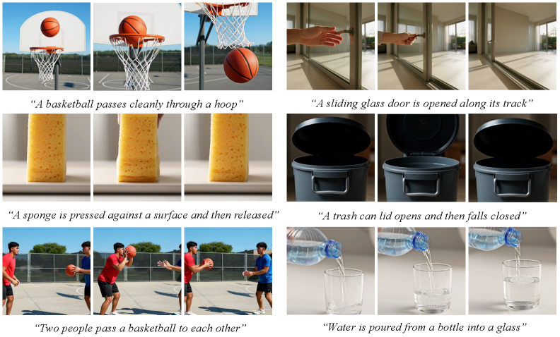
5.2 Qualitative Results

Fig. 3 presents text-to-video samples generated by EVD on six diverse interaction prompts (ball-through-hoop, sliding door, sponge press/release, trash-can lid open/close, two-person pass, and liquid pouring). Across these cases, EVD exhibits consistent event-grounded behavior: state changes are causally initiated (motion begins after the triggering action), contact is coherent (interacting objects maintain plausible spatial relationships without interpenetration or teleportation), and postconditions are stable (the scene settles after the event rather than drifting).

Figure 3: Representative text-conditioned video generations from EVD. EVD produces coherent event-driven dynamics across a diverse set of interactions, including target-directed motion, constrained mechanisms, deformation and recovery, gravity-mediated closure, multi-agent coordination, and liquid transfer. These examples illustrate that EVD captures causally grounded state transitions beyond simple frame-to-frame motion synthesis.

5.3 Quantitative Results on EVD-Bench

Tables 1 and 2 report our headline quantitative results on EVD-Bench, combining human preference (2AFC) and automatic metrics (VBench). Across all prompts, DiT+EVD is preferred substantially more often than the DiT baseline under Text Faithfulness, Overall Quality, and especially Dynamics, indicating that EVD improves event realization and temporal coherence in a way that is visible to human raters. On automatic evaluation, EVD delivers a large gain on VBench Dynamics while keeping VBench Appearance essentially unchanged (and in some cases slightly improved), matching the intended behavior of the method: EVD targets interaction-grounded dynamics rather than trading off appearance. This separation is important in practice, since many baseline failure cases arise from non-causal or unstable state updates even when individual frames look realistic.

Table 1: Comparison of EVD with prior video generation baselines on EVD-Bench. Human evaluation reports the percentage of pairwise votes favoring EVD; automatic metrics are computed using VBench.

	Human Eval			Auto. Metrics
Method	Text Faith.	Quality	Dynamics	Appearance	Dynamics
CogVideo2B	80.2	88.1	89.7	69.8	87.6
CogVideo5B	65.4	73.8	72.5	72.3	89.2
PyramidFlow	75.8	82.4	81.1	73.9	88.5
DiT-4B	70.6	76.8	80.3	75.4	78.9
DiT-4B + EVD	88.9	91.3	96.4	76.2	94.8

Table 2: Comparison of EVD with leading large-scale video generation models on EVD-Bench. Human evaluation reports the percentage of pairwise votes favoring EVD; automatic metrics are computed using VBench.

	Human Eval			Auto. Metrics
Method	Text Faith.	Quality	Dynamics	Appearance	Dynamics
Kling 3.0 Pro	61.8	67.4	72.9	78.6	92.6
Runway Gen-4.5	64.7	71.2	76.8	76.9	91.4
Veo 3.1	66.9	73.5	78.4	77.2	91.8
Sora 2 Pro	63.5	69.8	74.1	77.8	90.9
Mochi 1	58.2	63.7	70.3	72.6	88.8
DiT-30B	72.4	76.1	79.5	73.8	88.7
DiT-30B + EVD	89.7	92.4	97.1	78.1	95.7

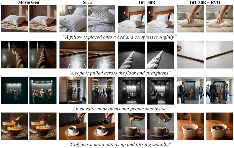
5.4 Baseline Comparisons

Fig. 4 shows qualitative comparisons on four representative interaction prompts. Despite strong per-frame realism, the baselines frequently violate event causality: objects begin changing state before contact is established, the key interaction is only weakly realized (e.g., a deformation or constraint response is missing), or the scene drifts after the interaction should have terminated. These issues are visible across interaction types, including material transfer (coffee filling), compliance (pillow compression), constraint enforcement (rope straightening), and multi-agent transitions (elevator door opening and people stepping inside). In contrast, EVD consistently produces event-aligned state changes: motion initiates after the triggering action, evolves coherently during the interaction, and settles to a stable postcondition without residual drift, matching the intended causal structure of each prompt.

Figure 4: Qualitative comparison with leading video generation baselines. We compare EVD against Movie Gen, Sora, and DiT-30B on representative prompts involving soft-body deformation, flexible-object dynamics, structured scene interactions, and liquid transfer. Across all examples, baseline models often exhibit incomplete event realization, weak contact-response coupling, or implausible state evolution, whereas EVD produces temporally ordered interactions and more coherent physical outcomes.

5.5 Ablations and Sensitivity

Component ablations.

Table 3 summarizes ablations of EVD on EVD-Bench. Removing any core component degrades human preference and/or dynamics in a targeted way: dropping realization primarily reintroduces non-causal initiation (Contact Stability); dropping consistency increases interaction jitter and unstable outcomes (State Persistence); and removing ordering weakens settling behavior after events. Training-only EVD (no inference gating) and inference-only EVD (no event losses) each recover only a portion of the gains, indicating that EVD’s improvements come from the coupling of event-grounded training and event-driven sampling. Finally, constant gating without annealing substantially harms preference despite strong automatic dynamics, motivating the scheduled gate used in the full model. To disambiguate event grounding from generic motion masking, we (i) construct pseudo-event targets from localized latent change with explicit camera-motion suppression, and (ii) include motion-mask controls (external motion gating / inference-only gating) showing smaller gains than full EVD; details are in Appendix 0.A.12.

Hyperparameter sensitivity.

EVD is broadly robust to $K$ (NFE), CFG scale $w_{\mathrm{cfg}}$, and gating hyperparameters $(\beta,\tau_{\mathrm{on}},\tau_{\mathrm{off}},t^{\star})$; we provide the full sensitivity sweep in Appendix 0.A.9.2 (Table 5).

Efficiency and Overhead

EVD preserves the backbone, solver, decoding stack, and sampling budget ($K$/NFE), and only gates the direction field; detailed parameter and runtime overhead are reported in Appendix 0.A.8.5 (Table 4).

Table 3: EVD ablations on EVD-Bench (DiT-4B backbone). Human Eval reports the percentage of 2AFC votes favoring the full DiT-4B+EVD model over each ablated variant (higher is better for EVD). Auto. Metrics are computed using VBench. All variants use identical sampling settings (solver, NFE, CFG scale) and the same prompt set.

	Settings					Human Eval (EVD wins %)			Auto. Metrics
Variant	Real	Cons	Order	Gate	Sched.	Text Faith.	Quality	Dynamics	Appearance	Dynamics
DiT-4B (no EVD)	No	No	No	No	–	70.6	76.8	80.3	75.4	78.9
w/o event realization	No	Yes	Yes	Yes	Anneal	65.2	69.4	78.8	75.9	91.2
w/o event consistency	Yes	No	Yes	Yes	Anneal	61.3	65.0	74.2	76.0	92.1
Training-only (no gating)	Yes	Yes	Yes	No	Off	63.0	66.8	77.1	76.1	90.5
Inference-only (no event losses)	No	No	No	Ext.	Anneal	70.5	74.9	86.0	75.6	84.0
Disable gating & event use @inf.	Yes	Yes	Yes	No	–	67.8	71.6	82.4	75.5	86.7
No schedule (const. gate)	Yes	Yes	Yes	Yes	Const(1.0)	55.7	58.9	60.5	75.7	94.1
No schedule (weak const. gate)	Yes	Yes	Yes	Yes	Const(0.5)	57.9	61.0	65.8	76.1	93.6
DiT-4B + EVD (full)	Yes	Yes	Yes	Yes	Anneal	88.9	91.3	96.4	76.2	94.8

6 Conclusion

We introduced Event-Driven Video Generation (EVD), a minimal modification to pretrained video DiT models that enforces event-grounded state transitions via (i) event-aligned training losses and (ii) event-gated sampling. Across EVD-Bench, EVD improves interaction realism and causal dynamics while preserving appearance, yielding consistent gains in both human preference and automatic dynamics metrics.

Limitations.

EVD can still fail when the event signal is weak or ambiguous at the model’s operating resolution (e.g., small/occluded contacts, cluttered multi-object interactions, thin fluid effects, or dominant camera motion), which can underdetermine both pseudo-targets and the learned event head. Future work may address these regimes by incorporating object-centric or contact-aware representations, stronger motion disentanglement, and higher-resolution latent/video backbones.

Appendix 0.A Appendix

Table of Contents

0.A.1 Abbreviations and symbols

Abbreviations.

• EVD: Event-Driven Video Generation.

• DiT: Diffusion Transformer (video DiT backbone used as the base model).

• CFG: Classifier-Free Guidance.

• FM: Flow Matching.

• ODE: Ordinary Differential Equation (sampling view for rectified-flow / FM samplers).

• NFE: Number of Function Evaluations (sampling compute proxy).

• TAE: Temporal Autoencoder (video encoder/decoder used to map $x\leftrightarrow z$).

• 2AFC: Two-Alternative Forced Choice (human preference protocol).

Core variables.

• $x\in\mathbb{R}^{T\times H\times W\times 3}$: video clip in pixel space.

• $z=E(x)\in\mathbb{R}^{T^{\prime}\times H^{\prime}\times W^{\prime}\times C}$: latent video produced by the temporal autoencoder encoder $E$.

• $D(\cdot)$: temporal autoencoder decoder mapping latents back to pixels.

• $t\in[0,1]$: continuous diffusion/flow time; $\{t_{k}\}_{k=0}^{K}$ is the discretized sampling grid.

• $z_{0}\sim\mathcal{N}(0,I)$: Gaussian noise latent; $z_{1}$: clean latent.

• $z_{t}$: noised/interpolated latent at time $t$ (see Sec. 0.A.2).

• $y$: text prompt; $\varnothing$: null prompt used for CFG.

Backbone and tokenization.

• $u_{\theta}(z_{t},y,t)$: DiT backbone prediction of the base target at time $t$ (parameters $\theta$).

• $\mathbf{s}_{t}\in\mathbb{R}^{N\times d}$: patchified token sequence; $N$ tokens, width $d$.

• $\mathrm{Tok}(\cdot)$, $\mathrm{UnTok}(\cdot)$: patchify/unpatchify operators aligned with DiT tokenization.

Flow Matching and guidance.

• $\tau(z_{1},z_{0},t)$: base training target; in FM, this is the velocity $v_{t}$.

• $v_{t}=z_{1}-z_{0}$: FM velocity target under linear interpolation.

• $w_{\mathrm{cfg}}$: CFG scale.

• $\widehat{\tau}^{\mathrm{cfg}}$: CFG-combined backbone prediction.

Events and gating.

• $e_{t}\in\mathbb{R}^{N\times C_{e}}$: token-aligned event field with $C_{e}$ channels.

• $\hat{e}_{t}$: predicted event field; $\hat{a}_{t}=\sigma(\hat{e}_{t}^{(1)})\in[0,1]^{N}$ is the activity channel.

• $g_{\psi}(\cdot)$: event gate derived from event predictions (parameters $\psi$).

• $g_{k}$: gate on sampling step $k$; $\tau_{\mathrm{on}},\tau_{\mathrm{off}}$: hysteresis thresholds; $\beta$: gate sharpness.

• $\rho(t)$: inference annealing schedule; $t^{\star}$: cutoff controlling “strong-early” gating.

Losses.

• $\mathcal{L}_{\mathrm{base}}$: backbone base loss (FM regression).

• $\mathcal{L}_{\mathrm{real}}$: event realization loss (no event $\Rightarrow$ no update).

• $\mathcal{L}_{\mathrm{cons}}$: event consistency loss (event $\Rightarrow$ coherent update).

• $\mathcal{L}_{\mathrm{order}}$: ordering/termination loss (suppresses pre-event motion and post-event drift).

• $\lambda_{\mathrm{real}},\lambda_{\mathrm{cons}},\lambda_{\mathrm{order}}$: corresponding loss weights.

• $w(t)$: time-weighting function emphasizing early timesteps.

0.A.2 Backbone and Notation

0.A.2.1 Latent video representation and notation

We consider text-conditioned video generation where a clip is represented as a tensor $x\in\mathbb{R}^{T\times H\times W\times 3}$ with $T$ frames. Following standard practice in large-scale video diffusion/flow models, we operate in a compressed latent space using a temporal video autoencoder (e.g., VAE/TAE). Let $E(\cdot)$ and $D(\cdot)$ denote the encoder and decoder, respectively, and define the latent video

$$z=E(x),\qquad x\approx D(z),$$ (23)

where $z\in\mathbb{R}^{T^{\prime}\times H^{\prime}\times W^{\prime}\times C}$ has reduced spatial/temporal resolution.

We write the text prompt as $y$, encoded by a frozen text encoder into a sequence of text embeddings. The generative backbone is a Diffusion Transformer (DiT) operating on latent videos; we denote the network by $\,u_{\theta}(\cdot)$, parameterized by $\theta$.

Noising and training target.

EVD is compatible with common continuous-time formulations used in modern DiT video models. We adopt a generic continuous-time notation: a clean latent $z_{1}$ is interpolated with noise $z_{0}\sim\mathcal{N}(0,I)$ to obtain a noised latent $z_{t}$ at time $t\in[0,1]$,

$$z_{t}=\alpha(t)\,z_{1}+\sigma(t)\,z_{0},$$ (24)

for a chosen schedule $\alpha,\sigma$. The corresponding training target depends on the base model (diffusion-score, velocity/flow-matching, or rectified flow); we denote it abstractly as $\tau(z_{1},z_{0},t)$. The DiT backbone is trained to predict $\tau$ from $(z_{t},y,t)$,

$$\mathcal{L}_{\text{base}}(\theta)=\mathbb{E}_{z_{1},z_{0},t,y}\Big[\big\|u_{\theta}(z_{t},y,t)-\tau(z_{1},z_{0},t)\big\|_{2}^{2}\Big].$$ (25)

All EVD components introduced in later subsections are built on top of this backbone objective and sampling procedure.

0.A.2.2 DiT-30B backbone summary (tokenization, spatiotemporal blocks, text conditioning)

EVD is built on a large video Diffusion Transformer (DiT) operating in latent space. Given a noised latent video $z_{t}\in\mathbb{R}^{T^{\prime}\times H^{\prime}\times W^{\prime}\times C}$, the backbone maps $(z_{t},y,t)$ to a prediction $u_{\theta}(z_{t},y,t)$ of the base training target (Sec. 0.A.2.1).

Patchification and token embeddings.

We partition $z_{t}$ into non-overlapping spatiotemporal patches of size $p_{t}\times p_{h}\times p_{w}$, flatten each patch, and linearly project it into the model width $d$, yielding a token sequence

$$\mathbf{s}_{t}=\mathrm{PatchEmbed}(z_{t})\in\mathbb{R}^{N\times d},$$ (26)

where $N=(T^{\prime}/p_{t})(H^{\prime}/p_{h})(W^{\prime}/p_{w})$. We add a learned spatiotemporal positional encoding $\mathrm{PE}\in\mathbb{R}^{N\times d}$ and a time embedding $\gamma(t)\in\mathbb{R}^{d}$ (broadcast to all tokens) to obtain the transformer input.

Spatiotemporal transformer blocks.

The backbone consists of $L$ blocks of multi-head self-attention and MLP layers applied to $\mathbf{s}_{t}$, with residual connections and normalization. We write the block update abstractly as

$$\mathbf{s}_{t}^{(\ell+1)}=\mathrm{Block}^{(\ell)}\!\left(\mathbf{s}_{t}^{(\ell)},\,\gamma(t),\,\phi(y)\right),\qquad\ell=0,\dots,L-1,$$ (27)

where $\phi(y)$ denotes the text conditioning (described below). The self-attention mixes information across both space and time by attending over the full spatiotemporal token set.

Text conditioning.

Text $y$ is encoded into a sequence of text embeddings $\phi(y)\in\mathbb{R}^{M\times d_{y}}$ using a frozen text encoder. The DiT conditions on $\phi(y)$ via cross-attention (or equivalently, attention over a concatenated key/value memory), so that each video token can attend to the prompt representation while preserving spatiotemporal structure.

Unpatchification and output projection.

After the final block, tokens are linearly projected back to patch space and unpatchified to recover a latent-shaped tensor $\widehat{u}\in\mathbb{R}^{T^{\prime}\times H^{\prime}\times W^{\prime}\times C}$. This $\widehat{u}$ is interpreted according to the base objective (e.g., velocity/flow target, score, or noise prediction) and is used for training and sampling.

Sampling interface (for later EVD modifications).

At inference, the backbone is evaluated repeatedly along a discretized time grid $\{t_{k}\}$, and an ODE/SDE solver (or discrete update) uses $u_{\theta}(z_{t_{k}},y,t_{k})$ to update the latent trajectory $\{z_{t_{k}}\}$. EVD will modify what the backbone is trained to represent (event grounding) and how its predictions are used during sampling (event-driven updates), while keeping the DiT backbone unchanged.

0.A.2.3 Base training objective (Flow Matching)

In our implementation, the DiT-30B backbone is trained with a continuous-time Flow Matching objective in latent space. Let $z_{1}=E(x)$ denote the clean latent video and $z_{0}\sim\mathcal{N}(0,I)$ denote Gaussian noise. For a timestep $t\sim\mathcal{U}[0,1]$, we form the interpolated latent

$$z_{t}=t\,z_{1}+(1-t)\,z_{0}.$$ (28)

The corresponding velocity target is the time derivative of the interpolation,

$$v_{t}\;=\;\frac{dz_{t}}{dt}\;=\;z_{1}-z_{0},$$ (29)

which is constant with respect to $t$ under the linear interpolation above. The DiT backbone $u_{\theta}(\cdot)$ is optimized to predict $v_{t}$ from $(z_{t},y,t)$ using an $\ell_{2}$ regression loss:

$$\mathcal{L}_{\mathrm{FM}}(\theta)=\mathbb{E}_{z_{1},\,z_{0},\,t,\,y}\Big[\big\|u_{\theta}(z_{t},y,t)-v_{t}\big\|_{2}^{2}\Big].$$ (30)

Compatibility.

While we describe EVD using Flow Matching notation for concreteness, the EVD components introduced in the sequel (event representation, event-grounded losses, and event-driven sampling) apply to other parameterizations (e.g., noise prediction or score prediction) by replacing the target in (30) with the corresponding base objective.

0.A.2.4 Sampling, guidance, and evaluation conventions

We summarize the sampling interface of the DiT-30B backbone and the conventions we use for guidance and evaluation. Unless otherwise stated, all models generate fixed-length clips (128 frames at 24 fps) in the latent space of a temporal autoencoder (TAE), followed by decoding to pixel space [4]. The TAE design follows the Movie Gen temporal autoencoder specification [22].

Time discretization and number of function evaluations (NFE).

Sampling proceeds by evolving a latent trajectory $\{z_{t_{k}}\}_{k=0}^{K}$ along a monotone time grid $0=t_{0}<t_{1}<\dots<t_{K}=1$. Each step queries the backbone once (or more, depending on guidance batching), so the total NFE scales with $K$ times the number of model evaluations per step. In practice, we report results at fixed $K$ to ensure fair comparisons across methods.

Classifier-free guidance (CFG).

We follow standard CFG conventions: at each step $t_{k}$, we evaluate the model with the prompt $y$ and with a null prompt $\varnothing$, and combine the predictions with a guidance scale $w\geq 0$:

$$u_{\mathrm{cfg}}(z_{t_{k}},y,t_{k})=(1+w)\,u_{\theta}(z_{t_{k}},y,t_{k})\;-\;w\,u_{\theta}(z_{t_{k}},\varnothing,t_{k}).$$ (31)

We use the same $w$ across all compared methods unless noted.

Batching for multi-condition guidance.

When multiple conditioning signals are used at inference (e.g., conditional/unconditional CFG and additional auxiliary conditions), the corresponding model evaluations can be executed as a single batched forward pass for efficiency. This follows standard CFG-style implementations and their multi-condition extensions (e.g., composable guidance and IP2P-style formulations) [5, 16, 3, 4].

Guidance scheduling over timesteps.

For guidance signals that primarily shape coarse spatiotemporal structure, concentrating guidance in early denoising steps is often beneficial, since these steps largely determine global dynamics. For example, VideoJAM applies its motion guidance only during the first half of generation (50 steps), motivated by the observation that coarse motion is set early [4]. EVD adopts the same principle: event-focused guidance is applied strongly in early steps and annealed thereafter (Sec. 0.A.7.3), while text CFG is applied throughout [5].

Evaluation protocol.

Unless explicitly stated, we generate one sample per prompt per model under identical sampling settings and a fixed random seed, and report both automatic scores (VBench) and human preference results; we use the first obtained sample for each prompt (no cherry-picking) [4, 9, 19]. For human evaluation, we follow a standard two-alternative forced-choice (2AFC) setup in which raters compare our output against a baseline and select the better video along text faithfulness, overall quality, and dynamics [24, 2].

0.A.3 EVD

0.A.3.1 Core claim: event-driven state transitions

Modern video generators often produce locally smooth frame-to-frame motion while violating basic causal structure: objects may move without contact, effects may precede causes, and post-interaction states may drift. EVD addresses this by enforcing a simple modeling principle:

A video is generated as a sequence of event-driven state transitions: persistent state evolves only when an event occurs, and events must be realized as consistent state changes.

State and event variables.

Let $z_{t}\in\mathbb{R}^{T^{\prime}\times H^{\prime}\times W^{\prime}\times C}$ denote the latent video state at diffusion/flow time $t$, and let $e_{t}$ denote an event representation aligned to the same time (Sec. 0.A.4.1). Intuitively, $z_{t}$ carries appearance and scene configuration, while $e_{t}$ encodes the presence and phase of an interaction (e.g., initiation, continuation, termination) that should drive changes in $z_{t}$.

Event grounding principle.

EVD implements two coupled constraints during learning and sampling:

(i) No-event $$\Rightarrow e_{t}\approx\mathbf{0}\;\Longrightarrow\;\Delta z_{t}\approx\mathbf{0},$$ no-update: (32)

(ii) Event $$\Rightarrow e_{t}\not\approx\mathbf{0}\;\Longrightarrow\;\Delta z_{t}\text{ reflects the event semantics.}$$ realized update: (33)

These principles directly target the two degeneracies commonly observed in frame-first generation: missing events (state changes without an initiating interaction) and ghost events (an apparent action with no coherent outcome).

Event-driven update rule (high-level).

Let $u_{\theta}(z_{t},y,t)$ denote the backbone prediction (Sec. 0.A.2). EVD uses a gated update interface of the form

$$\Delta z_{t}\;=\;g_{\psi}(e_{t},t)\,\odot\,u_{\theta}(z_{t},y,t),$$ (34)

where $g_{\psi}(\cdot)\in[0,1]$ is an event gate (scalar, per-token, or per-patch) derived from the event representation, and $\odot$ denotes elementwise modulation. When $e_{t}$ indicates “no interaction”, the gate suppresses spurious changes; when $e_{t}$ indicates an active event, the gate amplifies and stabilizes the corresponding state transition. The exact forms of $e_{t}$ and $g_{\psi}$ are specified in Secs. 0.A.4–0.A.4.4 and Secs. 0.A.7–0.A.7.3.

Connection to observed failure modes.

The event grounding constraints in (32)–(33) unify the four failure categories used in our analysis: State Persistence (termination without drift), Spatial Accuracy (event outcome aligns with target), Support Relations (valid load-bearing configurations), and Contact Stability (cause precedes motion and settling is stable). EVD is designed so that these behaviors emerge from the same mechanism: explicit event representation coupled to state updates.

0.A.3.2 What changes vs. vanilla DiT

EVD preserves the DiT-30B backbone (tokenization, attention blocks, and text conditioning) and modifies only the representation, objective, and sampling interface to make generation event-driven.

(1) Add an event representation.

In addition to the latent video state $z_{t}$, EVD introduces an event variable $e_{t}$ aligned with the same diffusion/flow time. Depending on the variant, $e_{t}$ can be implemented as (i) a dense event map in latent patch space or (ii) a compact set of event tokens. The role of $e_{t}$ is to explicitly encode whether an interaction is active and its phase (initiation/progression/termination).

(2) Train with event-grounded losses.

Vanilla DiT minimizes the base objective $\mathcal{L}_{\mathrm{FM}}$ (Sec. 0.A.2.3). EVD augments this with two lightweight constraints: (i) event realization to discourage state changes when no event is present, and (ii) event consistency to ensure that predicted events correspond to coherent state evolution. These terms are designed to eliminate both “missing events” and “ghost events” (Sec. 0.A.3.1).

(3) Use event-driven sampling.

At inference, vanilla DiT applies text guidance (CFG) and updates $z_{t}$ using the backbone prediction. EVD modifies the update using an event gate $g_{\psi}(e_{t},t)$ (Eq. (34)) so that event confidence controls when and where the latent state is allowed to change. This produces stable post-interaction states (no drift), sharper causal initiation (no pre-contact motion), and more reliable completion of interaction outcomes (e.g., correct placement/alignment).

Net effect.

EVD does not aim to “smooth motion”; it enforces event-grounded state transitions. As a result, improvements concentrate on dynamics-related metrics and human preference for physically coherent interactions, while appearance metrics typically change only modestly.

0.A.3.3 Mapping EVD components to failure modes

We use four failure categories throughout the paper—State Persistence, Spatial Accuracy, Support Relations, and Contact Stability—and design EVD so that each category is addressed by an explicit mechanism rather than emergent smoothing. Below we summarize the correspondence between the observed failures (Fig. 2) and EVD’s components (Secs. 0.A.4–0.A.7).

State Persistence (terminate $\Rightarrow$ rest).

Failure signature: objects continue drifting or jittering after an interaction ends (e.g., residual chair motion). EVD targets this via event termination in the event representation $e_{t}$ and the no-event $\Rightarrow$ no-update constraint (Eq. (32)). Concretely, once $e_{t}$ indicates the event has ended, the event gate suppresses further latent updates, preventing post-interaction drift. The event-realization loss further discourages nonzero updates when $e_{t}$ is near zero.

Spatial Accuracy (outcome aligns with target).

Failure signature: misaligned outcomes (e.g., placement misses a platform, offsets accumulate). EVD encourages outcome-conditioned updates by coupling $e_{t}$ to state changes through gated modulation (Eq. (34)). During training, the event-consistency loss penalizes event predictions that do not produce the corresponding state change toward a stable, target-consistent configuration, sharpening alignment at event completion.

Support Relations (valid load-bearing configurations).

Failure signature: stacked objects appear without a placing action, or settle into physically inconsistent configurations. EVD addresses this in two ways: (i) event realization discourages “teleportation” of support relationships (stacking without a placement event); (ii) event consistency ties the predicted event phase to a coherent progression of the state (approach $\rightarrow$ contact $\rightarrow$ release), encouraging stable postconditions rather than instantaneous, unsupported transitions.

Contact Stability (cause precedes motion; stable settling).

Failure signature: motion begins before contact, contact is visually absent, or settling remains unstable (sliding/drifting). EVD explicitly models causal initiation by requiring $e_{t}$ to activate before allowing the corresponding update ($g_{\psi}(e_{t},t)$ increases only when an initiating interaction is present). This reduces pre-contact motion. In addition, the gate is annealed after event completion to promote stable settling, aligning with the “contact then rest” structure of many prompts.

Takeaway.

All four categories are handled through a unified design: learn an event representation $e_{t}$ and use it to (i) constrain which latent updates are permitted and (ii) penalize mismatches between event signals and state evolution. This shifts the model from frame-to-frame correlation toward event-grounded state transitions.

0.A.4 Event Representation and Supervision

0.A.4.1 What is an “event” in EVD?

EVD models a video as persistent latent state punctuated by events that induce structured state changes. Informally, an event is the minimal interaction that explains a meaningful transition in the scene—e.g., contact is made, an object is released, a constraint becomes active (hinge/track), or material is transferred (pouring).

Event as a typed, phased interaction.

We represent events with two ingredients: (i) an activity signal indicating whether an interaction is currently active, and (ii) a phase signal indicating where the interaction lies along an initiation-to-termination progression. Concretely, for each diffusion/flow time $t$, we define an event representation

$$e_{t}\;\triangleq\;\big(a_{t},\;p_{t},\;\kappa_{t}\big),$$ (35)

where $a_{t}\in[0,1]$ is an event activity score, $p_{t}\in[0,1]$ is an event phase (early $\rightarrow$ late), and $\kappa_{t}$ encodes event type (e.g., contact/transfer/deformation/constraint) when multiple interaction modes may occur. In the simplest variant, $\kappa_{t}$ is omitted and $e_{t}=(a_{t},p_{t})$.

Spatial localization (where the event acts).

Because events are typically localized (e.g., hand–object contact, placement region, hinge boundary), EVD attaches event variables to the same spatiotemporal tokenization used by the DiT backbone. Let $\mathrm{PatchEmbed}(z_{t})$ produce $N$ tokens (Sec. 0.A.2.2). We define a token-aligned event field

$$e_{t}\in\mathbb{R}^{N\times C_{e}},$$ (36)

where $C_{e}$ is small (e.g., $C_{e}\in\{1,2,4\}$). The activity component $a_{t}$ can be interpreted as a per-token gate, while $p_{t}$ captures local event progress. This alignment allows EVD to modulate updates where an interaction occurs, rather than globally smoothing the entire video.

Event-grounded state transitions.

EVD uses $e_{t}$ to constrain state evolution in latent space: event activity determines whether updates are permitted, and event phase shapes when updates should begin and terminate. This directly targets the two dominant failure modes in frame-first generation: (i) missing events (state changes without an interaction) and (ii) ghost events (an apparent interaction with no coherent state change).

0.A.4.2 Event signals used in EVD

EVD supports multiple instantiations of the event representation $e_{t}$, trading off expressivity, overhead, and ease of integration with a pretrained DiT-30B backbone. We describe three practical variants; in all cases, $e_{t}$ is aligned with the DiT tokenization so it can modulate latent updates at the appropriate spatiotemporal locations.

(i) Dense event field (per-token event map).

The default EVD representation is a dense event field

$$e_{t}\in\mathbb{R}^{N\times C_{e}},$$ (37)

where $N$ is the number of spatiotemporal tokens and $C_{e}$ is small (typically 1–4). A minimal choice is $C_{e}=1$, where $e_{t}$ encodes activity only. A slightly richer choice is $C_{e}=2$, where $e_{t}=(a_{t},p_{t})$ encodes both event activity $a_{t}\in[0,1]$ and phase $p_{t}\in[0,1]$. This variant is lightweight, fully local, and directly supports event gating $g_{\psi}(e_{t},t)$ (Sec. 0.A.7.2).

(ii) Sparse event tokens (compact event memory).

For interactions that are semantically global but spatially sparse (e.g., a single handoff or a single placement), EVD can instead represent events as a small set of learned tokens

$$e_{t}^{\mathrm{tok}}\in\mathbb{R}^{K_{e}\times d},\qquad K_{e}\ll N,$$ (38)

and inject them via cross-attention into the DiT backbone. This yields a compact “event memory” that conditions the video tokens, while a separate projection produces a token-aligned activity gate $\tilde{a}_{t}\in[0,1]^{N}$ used for update modulation. In practice, this variant is useful when compute is tight and events are few.

(iii) Scalar event progress (global activity/phase).

For ablations and the simplest deployments, EVD can use a global event descriptor

$$e_{t}^{\mathrm{glob}}=(a_{t}^{\mathrm{glob}},p_{t}^{\mathrm{glob}})\in[0,1]^{2},$$ (39)

shared across all tokens. This captures “whether something is happening” and “how far along it is” but cannot localize interactions. We include this variant mainly as a diagnostic baseline; it improves gross temporal ordering but is weaker on spatially localized contacts.

Which variant we use.

Unless noted otherwise, our 30B results use the dense event field $e_{t}\in\mathbb{R}^{N\times C_{e}}$ with a small channel budget. This choice provides a direct interface for (a) suppressing spurious updates outside interaction regions and (b) enforcing event termination to stabilize the post-interaction state, while adding negligible overhead relative to the DiT-30B backbone.

0.A.4.3 How event targets are obtained (self-supervised extraction)

EVD does not require manual event annotations. Instead, we derive pseudo-targets for event activity and phase directly from the training videos using lightweight, off-the-shelf signals that capture when and where meaningful change occurs.

Inputs and alignment.

Given a training clip $x$ and its latent $z_{1}=E(x)$, we compute event pseudo-targets at the same spatiotemporal granularity as the DiT tokens. In practice, we operate either (i) on decoded frames $\tilde{x}=D(z_{1})$ at the autoencoder resolution or (ii) directly on latent differences, and then downsample/aggregate to the patch grid, yielding a token-aligned event field $e_{t}^{\star}\in\mathbb{R}^{N\times C_{e}}$.

Activity target (“is an interaction happening?”).

We estimate a dense motion/change magnitude signal and convert it into an activity map. A simple and robust choice is to use optical flow magnitude between consecutive frames (or a latent-space proxy). Let $F_{\tau}$ denote an off-the-shelf flow estimator (e.g., RAFT is a common choice for large-scale pipelines) :contentReference[oaicite:0]index=0 and let $f_{\tau}=F_{\tau}(\tilde{x}_{\tau},\tilde{x}_{\tau+1})$. Define the per-pixel magnitude $m_{\tau}=\|f_{\tau}\|_{2}$. We then map this to an activity probability via a soft threshold:

$$a_{\tau}^{\star}(u)=\sigma\!\left(\frac{m_{\tau}(u)-\mu}{s}\right),$$ (40)

where $\sigma(\cdot)$ is the logistic sigmoid, $\mu$ is a robust scale (e.g., median magnitude), and $s$ controls softness. Finally, we aggregate $a_{\tau}^{\star}$ to the DiT patch grid (average pooling over pixels and frames within each patch) to obtain $a_{\tau}^{\star}\in[0,1]^{N}$.

Phase target (“where are we within the interaction?”).

For many prompts, a single dominant interaction admits a canonical progression from initiation to termination. We construct a normalized phase signal from the cumulative activity:

$$p_{\tau}^{\star}=\frac{\sum_{j=0}^{\tau}\langle a_{j}^{\star},\mathbf{1}\rangle}{\sum_{j=0}^{T-1}\langle a_{j}^{\star},\mathbf{1}\rangle+\varepsilon},$$ (41)

where $\langle a_{j}^{\star},\mathbf{1}\rangle$ sums activity over tokens and $\varepsilon$ avoids division by zero. This yields $p_{\tau}^{\star}\in[0,1]$ that increases smoothly over the event and saturates afterward. When multiple disjoint interactions exist, we compute phase locally per-token (by normalizing within spatial neighborhoods) to avoid forcing unrelated regions to share a global phase.

Event-type cues.

When we instantiate a multi-channel event type $\kappa_{t}$ (Sec. 0.A.4.1), we assign coarse types using simple diagnostics on the same signals: e.g., large localized activity near boundaries suggests contact/impact, sustained constrained motion suggests mechanism/track, and spatially diffuse change suggests material transfer. These cues remain self-supervised and are used only as weak targets.

Takeaway.

The pseudo-targets $e_{t}^{\star}=(a_{t}^{\star},p_{t}^{\star},\kappa_{t}^{\star})$ provide a lightweight supervisory signal that teaches the model when and where changes should occur, without requiring any additional human labeling.

0.A.4.4 Event confidence and uncertainty (and how it is used)

In practice, event pseudo-targets are noisy: flow-based change can be triggered by camera motion, texture flicker, or small background dynamics. EVD therefore associates each event estimate with a confidence signal that controls how strongly event grounding is enforced during training and sampling.

Confidence score.

Given a token-aligned activity target $a_{t}^{\star}\in[0,1]^{N}$ (Sec. 0.A.4.3), we define a scalar confidence $\,c_{t}^{\star}\in[0,1]$ as a robust summary of activity concentration:

$$c_{t}^{\star}\;=\;\mathrm{clip}\!\Big(\mathrm{mean}_{i\in\mathcal{I}_{t}}\,a_{t}^{\star}(i),\,0,\,1\Big),\qquad\mathcal{I}_{t}\;=\;\{i:a_{t}^{\star}(i)\geq\tau_{a}\},$$ (42)

where $\tau_{a}$ is a small threshold (0.3) and $\mathcal{I}_{t}$ selects the most active tokens. Intuitively, $c_{t}^{\star}$ is high when the interaction is spatially localized and unambiguous, and low when the activity is diffuse or weak.

Training usage: loss weighting.

We weight event-grounded auxiliary losses by confidence to avoid over-regularizing ambiguous regions:

$$\mathcal{L}\;=\;\mathcal{L}_{\mathrm{FM}}\;+\;\lambda_{\mathrm{real}}\,c_{t}^{\star}\,\mathcal{L}_{\mathrm{real}}\;+\;\lambda_{\mathrm{cons}}\,c_{t}^{\star}\,\mathcal{L}_{\mathrm{cons}},$$ (43)

so that event grounding is emphasized when the extracted event signal is reliable.

Inference usage: adaptive gating and guidance.

At sampling time, we similarly modulate the strength of event-driven updates by a confidence-weighted schedule:

$$g_{\psi}(e_{t},t)\;=\;\underbrace{\rho(t)}_{\text{early-step emphasis}}\cdot\underbrace{\tilde{c}_{t}}_{\text{model/event confidence}}\cdot\underbrace{\sigma\!\big(\beta\,a_{t}\big)}_{\text{activity gate}},$$ (44)

where $\rho(t)$ is a monotonically decreasing schedule (strong early, weak late), $\tilde{c}_{t}$ is the model’s predicted confidence (trained to match $c_{t}^{\star}$), and $\beta$ controls gate sharpness. This ensures that strong event gating is applied primarily when the model is confident an interaction is occurring, reducing the risk of suppressing legitimate motion in challenging scenes.

Calibration.

We calibrate $\tilde{c}_{t}$ using a temperature parameter on a held-out set (or simple clipping), so that confidence reflects the empirical reliability of event predictions and remains comparable across prompts.

0.A.5 Architecture: Adding Events to DiT-30B

0.A.5.1 Conditioning pathway: injecting events into the DiT backbone

EVD preserves the DiT-30B transformer blocks and introduces an event pathway that (i) produces a token-aligned event representation $e_{t}$ and (ii) injects it into the backbone as an additional conditioning signal. We design the injection to be lightweight and to preserve the pretrained behavior at initialization via zero-impact conditioning (e.g., zero-initialized projections / appended zero-rows), following the same stability principle used in DiT-based video adaptations [21, 4] and in conditional-control networks for diffusion models [28]. When a parameter-efficient variant is desired, the same event pathway can be implemented with low-rank adapters on attention/MLP projections [7].

Event module.

Given the noised latent $z_{t}$, prompt $y$, and time $t$, an event module $h_{\psi}$ produces a token-aligned event field

$$e_{t}\;=\;h_{\psi}(z_{t},y,t)\in\mathbb{R}^{N\times C_{e}},$$ (45)

where $N$ is the number of spatiotemporal tokens induced by patchification and $C_{e}$ is small (Sec. 0.A.4).

Input-level event injection (default).

Let $\mathbf{s}_{t}=\mathrm{PatchEmbed}(z_{t})\in\mathbb{R}^{N\times d}$ be the DiT token sequence (Sec. 0.A.2.2). We embed the event field into the same width $d$ via a linear map $W_{e}\in\mathbb{R}^{C_{e}\times d}$ and add it as a token-wise bias:

$$\mathbf{s}_{t}^{(0)}\;=\;\mathbf{s}_{t}\;+\;\eta(t)\,\big(e_{t}W_{e}\big),$$ (46)

where $\eta(t)$ is a (possibly scheduled) scalar controlling event-conditioning strength. We initialize $W_{e}$ to zero (or initialize $\eta(t)=0$) so that the model reduces exactly to the pretrained backbone at step 0, and event conditioning is learned during fine-tuning.

Alternative: channel concatenation with zero-init projection.

In an equivalent implementation, we concatenate a projected event tensor to the latent channels prior to patchification (Sec. 0.A.2.2), $\tilde{z}_{t}=[z_{t},\;\Pi(e_{t})]$, and extend the input projection with zero-initialized rows so that the pretrained mapping is preserved at initialization [4, 29]. This variant is convenient when the codebase already supports multi-channel latent inputs.

Mid-block modulation.

For tighter control of where/when events affect computation, we use FiLM-style modulation inside each transformer block:

$$\mathrm{Norm}(\mathbf{s})\;\mapsto\;\gamma_{\ell}(e_{t},t)\odot\mathrm{Norm}(\mathbf{s})\;+\;\beta_{\ell}(e_{t},t),$$ (47)

where $\gamma_{\ell},\beta_{\ell}$ are shallow MLPs applied token-wise to $[e_{t};\gamma(t)]$. We use this only in the 30B setting when the qualitative gains justify the additional parameters; otherwise the input-level injection (Eq. (46)) suffices.

Text conditioning unchanged.

Text embeddings $\phi(y)$ are consumed by the DiT via the existing cross-attention pathway; EVD does not alter the text encoder or the prompt-conditioning interface.

Summary.

EVD adds an event pathway that produces $e_{t}$ and injects it into the DiT token stream with zero-initialized conditioning, ensuring stable fine-tuning of a pretrained 30B backbone while enabling event-aware computation.

0.A.5.2 Output parameterization: state update and event prediction

EVD keeps the DiT backbone prediction interface for the state update (the base training target), and adds a lightweight event head that predicts the event representation used for grounding and gating.

State prediction (unchanged).

Let $\widehat{\tau}_{t}=u_{\theta}(z_{t},y,t)$ denote the DiT prediction of the base target $\tau(z_{1},z_{0},t)$ (e.g., the Flow Matching velocity $v_{t}$; Sec. 0.A.2.3). This prediction is used exactly as in the pretrained backbone during both training and sampling, except that EVD modulates its effect on the latent update via an event gate (Sec. 0.A.7.2).

Event prediction.

To obtain an explicit event variable aligned with the DiT tokenization, we attach a small projection head to the final DiT token features. Let $\mathbf{s}_{t}^{(L)}\in\mathbb{R}^{N\times d}$ be the final token sequence produced by the transformer. We predict a token-aligned event field $\hat{e}_{t}\in\mathbb{R}^{N\times C_{e}}$ using a linear layer (or a 2-layer MLP):

$$\hat{e}_{t}\;=\;\pi_{\psi}\!\left(\mathbf{s}_{t}^{(L)},t\right),\qquad\pi_{\psi}(\mathbf{s},t)\;=\;\mathrm{MLP}_{\psi}\!\big([\mathbf{s};\gamma(t)]\big)\,,$$ (48)

where $\gamma(t)$ is the standard time embedding. We typically interpret the first channel as an activity logit and additional channels as phase/type descriptors (Sec. 0.A.4.1).

Joint prediction view.

It is often convenient to view the model as producing a joint output

$$u_{\theta,\psi}(z_{t},y,t)\;=\;\big(\widehat{\tau}_{t},\;\hat{e}_{t}\big),$$ (49)

where $\widehat{\tau}_{t}$ drives the state evolution and $\hat{e}_{t}$ provides the event grounding signal used for both auxiliary losses (Sec. 0.A.6) and event-driven sampling (Sec. 0.A.7).

Initialization and stability.

To preserve the pretrained DiT behavior at the beginning of fine-tuning, we initialize the event head $\pi_{\psi}$ to near-zero output (e.g., small weights), so that the event pathway does not perturb the backbone prediction initially. This follows a common “no-op at initialization” design used when attaching new conditioning/residual branches to large pretrained generators, including zero-initialized control branches in diffusion models [29], lightweight DiT-video adaptations that preserve the pretrained mapping at initialization [4], and parameter-efficient adapter layers that are initialized to behave close to the identity [6].

When to omit the event head.

For ablations or strict minimalism, one may compute $e_{t}$ purely from an external extractor on decoded frames (Sec. 0.A.4.3). However, we find that predicting $\hat{e}_{t}$ directly from the DiT features yields the strongest gains, since it lets the model learn an event representation aligned with its own latent geometry and sampling trajectory.

0.A.5.3 Parameter budget options (and what we use at 30B)

EVD is designed to be compatible with large pretrained DiT backbones under different adaptation budgets. We summarize three practical configurations, ordered from minimal overhead to maximal flexibility.

EVD-lite (lowest overhead).

This variant keeps the DiT backbone frozen (or lightly tuned) and adds only: (i) the event injection parameters $W_{e}$ (Eq. (46)), (ii) the event head $\pi_{\psi}$ (Eq. (48)), and (iii) a small gating module $g_{\psi}$ used at sampling time (Sec. A.6). The additional parameters are $O(C_{e}d)$ for $W_{e}$ and $O(dC_{e})$ for the event head (often a single linear layer), which is negligible relative to a 30B backbone. EVD-lite is useful for rapid iteration and ablations, and already yields visible improvements on event fidelity.

EVD-adapter (moderate overhead).

Here we add lightweight adapters (e.g., LoRA or small bottleneck MLPs) to a subset of transformer blocks while keeping the base weights fixed. Event injection and the event head remain as in EVD-lite. This typically improves the alignment between the learned event representation and the backbone dynamics without the cost of full fine-tuning. In our experience, adapting attention projections in later blocks provides most of the benefit.

EVD-full (highest performance).

This variant fine-tunes the full DiT-30B weights jointly with the event modules. Although this is the most expensive option, it produces the strongest and most reliable gains on EVD-Bench, particularly for: (i) precise interaction outcomes (spatial accuracy), (ii) stable post-contact settling (contact stability), and (iii) “event realization” failures where the baseline skips the visible interaction.

What we report at 30B.

Unless otherwise stated, our main 30B results use EVD-full with: (a) dense event field $e_{t}\in\mathbb{R}^{N\times C_{e}}$, (b) input-level event injection (Eq. (46)), (c) a lightweight event head (Eq. (48)), and (d) event-driven sampling with early-step emphasis (Sec. 0.A.7). This choice yields the best trade-off between stability and performance at scale, while keeping architectural changes minimal.

0.A.5.4 Initialization and stability tricks for 30B fine-tuning

Fine-tuning a 30B DiT backbone is sensitive to even small interface changes. EVD therefore adopts conservative initialization and optimization choices so that training starts exactly from the pretrained generator and gradually introduces event grounding.

Zero-impact initialization.

We initialize the event pathway to have (near) zero effect on the pretrained forward pass: (i) the event injection projection $W_{e}$ in Eq. (46) is initialized to all zeros (or we set $\eta(t)\equiv 0$ at step 0), and (ii) the event head $\pi_{\psi}$ in Eq. (48) is initialized with small weights so that $\hat{e}_{t}\approx 0$ initially. This ensures the first optimization steps match the base DiT behavior before learning event structure.

Gradual event turn-on.

We ramp event influence using a short warm-up on the injection strength and auxiliary loss weights:

$$\eta(t)\leftarrow\eta(t)\cdot r(s),\qquad\lambda_{\mathrm{real}}\leftarrow\lambda_{\mathrm{real}}\cdot r(s),\qquad\lambda_{\mathrm{cons}}\leftarrow\lambda_{\mathrm{cons}}\cdot r(s),$$ (50)

where $s$ is the optimization step and $r(s)$ increases linearly from $0$ to $1$ over the warm-up window.

Event dropout (robustness).

To prevent the backbone from over-relying on a possibly noisy event signal early in training, we randomly drop the event conditioning with probability $p_{e}$ (set $e_{t}=\mathbf{0}$) and train the model to remain functional under missing event cues. This also stabilizes training when event pseudo-targets are uncertain (Sec. 0.A.4.4).

Two-group learning rates.

We use separate optimizer groups for stability:

• Backbone weights $\theta$: small learning rate (conservative), standard weight decay.

• New EVD modules $\psi$ (event injection/head/gate): larger learning rate, reduced or zero weight decay for biases/norms.

This keeps the pretrained representation intact while allowing the new event pathway to adapt quickly.

Gradient and precision safeguards.

We apply gradient clipping (global norm) to avoid rare spikes, maintain an EMA of weights for sampling stability, and use bf16/fp16 training with loss scaling as needed. When using full fine-tuning, activation checkpointing is enabled to keep memory bounded.

Sanity check: “no-regression” at initialization.

Before full training, we verify that with event influence disabled ($\eta=0$, $\lambda_{\mathrm{real}}=\lambda_{\mathrm{cons}}=0$), the fine-tuning code reproduces the base model outputs within numerical tolerance. This guards against silent interface bugs in 30B-scale runs.

0.A.6 Training Objective: Event-Grounded Dynamics Learning

0.A.6.1 Base loss recap

EVD is built on top of the pretrained DiT-30B training objective and preserves the original target parameterization. In our implementation, the backbone is trained with a Flow Matching regression objective in latent space (Sec. 0.A.2.3). We restate it here for completeness.

Given a clean latent video $z_{1}=E(x)$, Gaussian noise $z_{0}\sim\mathcal{N}(0,I)$, and a timestep $t\sim\mathcal{U}[0,1]$, we form the noised latent $z_{t}=tz_{1}+(1-t)z_{0}$ and velocity target $v_{t}=z_{1}-z_{0}$. The backbone $u_{\theta}$ is trained via

$$\mathcal{L}_{\mathrm{base}}(\theta)=\mathbb{E}_{z_{1},z_{0},t,y}\Big[\big\|u_{\theta}(z_{t},y,t)-v_{t}\big\|_{2}^{2}\Big].$$ (51)

EVD augments $\mathcal{L}_{\mathrm{base}}$ with event-grounded auxiliary terms that penalize (i) state updates without an event and (ii) events without a coherent state update. The full training objective is

$$\mathcal{L}(\theta,\psi)=\mathcal{L}_{\mathrm{base}}(\theta)+\lambda_{\mathrm{real}}\,\mathcal{L}_{\mathrm{real}}(\theta,\psi)+\lambda_{\mathrm{cons}}\,\mathcal{L}_{\mathrm{cons}}(\theta,\psi),$$ (52)

where $\psi$ denotes EVD-specific parameters (event injection/head/gate; Sec. A.4). We define $\mathcal{L}_{\mathrm{real}}$ (event realization) and $\mathcal{L}_{\mathrm{cons}}$ (event consistency) in Secs. 0.A.6.2–0.A.6.3. both terms can be weighted by event confidence and/or a timestep schedule to emphasize early-step dynamics (Sec. 0.A.4.4, Sec. 0.A.6.5).

0.A.6.2 Event realization loss (no event $\Rightarrow$ no state change)

The first auxiliary term enforces the principle that state changes should be explained by events. In practice, frame-first generators often exhibit “missing events”: the outcome appears without a visible interaction, or motion begins before any initiating contact. We penalize such behavior by suppressing backbone-predicted updates when the event activity is low.

Predicted event activity.

Let $\hat{e}_{t}\in\mathbb{R}^{N\times C_{e}}$ be the predicted event field (Eq. (48)). We extract an activity score $\hat{a}_{t}\in[0,1]^{N}$ from the first channel using a sigmoid:

$$\hat{a}_{t}\;=\;\sigma(\hat{e}_{t}^{(1)}),$$ (53)

where $\hat{e}_{t}^{(1)}$ denotes the first channel.

Gated update magnitude.

Let $\widehat{\tau}_{t}=u_{\theta}(z_{t},y,t)$ be the backbone prediction of the base target (e.g., velocity). We define a token-wise gated update magnitude by scaling $\widehat{\tau}_{t}$ in patch space. Concretely, let $\mathrm{Tok}(\widehat{\tau}_{t})\in\mathbb{R}^{N\times d_{\tau}}$ be the patchified form of $\widehat{\tau}_{t}$ (using the same patchification as the backbone), and define

$$\Delta_{t}^{\mathrm{pred}}\;=\;(1-\hat{a}_{t})\odot\mathrm{Tok}(\widehat{\tau}_{t}),$$ (54)

so that $\Delta_{t}^{\mathrm{pred}}$ captures the portion of the predicted update that occurs when the model claims no event is active.

Event realization penalty.

We penalize the magnitude of $\Delta_{t}^{\mathrm{pred}}$, encouraging the model to avoid changing the state outside event regions:

$$\mathcal{L}_{\mathrm{real}}(\theta,\psi)=\mathbb{E}_{z_{1},z_{0},t,y}\Big[\big\|\Delta_{t}^{\mathrm{pred}}\big\|_{2}^{2}\Big]=\mathbb{E}\Big[\big\|(1-\hat{a}_{t})\odot\mathrm{Tok}(u_{\theta}(z_{t},y,t))\big\|_{2}^{2}\Big].$$ (55)

This term does not suppress legitimate motion: when an event is active, $\hat{a}_{t}$ increases and the penalty vanishes.

Interpretation.

$\mathcal{L}_{\mathrm{real}}$ explicitly discourages “teleportation” in latent space: if the model predicts a state change, it must also predict an event signal that justifies it. This directly targets failures where objects move before contact, or outcomes appear without the corresponding interaction.

0.A.6.3 Event consistency loss (event $\Rightarrow$ coherent state update)

The second auxiliary term enforces the converse principle: when an event is predicted, the resulting state evolution should be coherent and consistent with that event. This targets “ghost events” where the model depicts an apparent interaction (e.g., a hand reaches toward an object) but the world state does not respond correctly (no lift, no settling, no constraint-respecting motion).

Event-phase and directionality.

When using a multi-channel event field $e_{t}=(a_{t},p_{t},\kappa_{t})$ (Sec. 0.A.4.1), the phase $p_{t}\in[0,1]$ provides a natural ordering signal: initiation $\rightarrow$ progression $\rightarrow$ termination. We extract a predicted phase $\hat{p}_{t}\in[0,1]^{N}$ from the second channel (when present),

$$\hat{p}_{t}\;=\;\sigma(\hat{e}_{t}^{(2)}),$$ (56)

and use it to enforce monotone, non-oscillatory event-driven updates. For the minimal $C_{e}=1$ setting (activity-only), we omit phase and use the activity-based variant described below.

Consistency as “directed change” under active events.

Let $\mathrm{Tok}(\widehat{\tau}_{t})\in\mathbb{R}^{N\times d_{\tau}}$ denote the patchified backbone prediction. Intuitively, when an event is active (high $\hat{a}_{t}$), we want the induced update to be stable and directed rather than jittery or sign-flipping. We implement this using a pairwise smoothness penalty across adjacent sampling times. Let $t$ and $t^{\prime}$ be two nearby timesteps (e.g., two sampled points on the discretized schedule), and let $\widehat{\tau}_{t}=u_{\theta}(z_{t},y,t)$, $\widehat{\tau}_{t^{\prime}}=u_{\theta}(z_{t^{\prime}},y,t^{\prime})$. We define an event-masked temporal consistency term

$$\mathcal{L}_{\mathrm{cons}}^{\mathrm{temp}}=\mathbb{E}\Big[\big\|\hat{a}_{t}\odot\mathrm{Tok}(\widehat{\tau}_{t})-\hat{a}_{t^{\prime}}\odot\mathrm{Tok}(\widehat{\tau}_{t^{\prime}})\big\|_{2}^{2}\Big],$$ (57)

which encourages the update predicted during an active event to evolve smoothly across time rather than oscillate.

Phase-aware consistency.

When phase is available, we additionally encourage the magnitude of the update to follow the phase progression: early in the event (small $\hat{p}_{t}$), motion begins; near termination (large $\hat{p}_{t}$), motion settles. A simple implementation is to penalize large updates late in the event:

$$\mathcal{L}_{\mathrm{cons}}^{\mathrm{phase}}=\mathbb{E}\Big[\big\|\hat{a}_{t}\odot\hat{p}_{t}\odot\mathrm{Tok}(\widehat{\tau}_{t})\big\|_{2}^{2}\Big],$$ (58)

which suppresses residual motion after the model indicates the event is near completion.

Final consistency loss.

We combine the above terms (using only the components relevant to the chosen event parameterization):

$$\mathcal{L}_{\mathrm{cons}}(\theta,\psi)=\mathcal{L}_{\mathrm{cons}}^{\mathrm{temp}}+\alpha_{\mathrm{ph}}\,\mathcal{L}_{\mathrm{cons}}^{\mathrm{phase}}.$$ (59)

Interpretation.

$\mathcal{L}_{\mathrm{cons}}$ ensures that predicted events correspond to stable, coherent state evolution: updates do not jitter during an active interaction and they naturally decay as the event terminates. Together with $\mathcal{L}_{\mathrm{real}}$, this couples events and state transitions bidirectionally: state change requires an event, and an event requires a coherent state change.

0.A.6.4 Ordering and termination regularization

Beyond coupling events and state updates, we add a lightweight regularizer to enforce causal ordering: initiation precedes motion and termination precedes rest. This directly targets failure cases where motion begins before contact or continues after the interaction has ended.

Initiation-before-update.

Let $\hat{a}_{t}\in[0,1]^{N}$ be the predicted event activity (Eq. (53)) and $\mathrm{Tok}(\widehat{\tau}_{t})$ be the patchified update prediction. We discourage nontrivial updates in tokens whose activity is below a small initiation threshold $\tau_{\mathrm{on}}$:

$$\mathcal{L}_{\mathrm{on}}=\mathbb{E}\Big[\big\|\mathbb{I}[\hat{a}_{t}<\tau_{\mathrm{on}}]\odot\mathrm{Tok}(\widehat{\tau}_{t})\big\|_{2}^{2}\Big],$$ (60)

where $\mathbb{I}[\cdot]$ is an indicator applied token-wise. This is a “harder” version of $\mathcal{L}_{\mathrm{real}}$ that explicitly enforces a causal onset.

Termination-before-rest.

Similarly, we penalize residual update energy after an event is predicted to be over. Using a termination threshold $\tau_{\mathrm{off}}$, we define

$$\mathcal{L}_{\mathrm{off}}=\mathbb{E}\Big[\big\|\mathbb{I}[\hat{a}_{t}<\tau_{\mathrm{off}}]\odot\mathrm{Tok}(\widehat{\tau}_{t})\big\|_{2}^{2}\Big],$$ (61)

with $\tau_{\mathrm{off}}$ typically chosen slightly smaller than $\tau_{\mathrm{on}}$ to introduce hysteresis (i.e., once an interaction is “off”, it stays off unless strong evidence reactivates it).

Phase-aware termination (when phase is available).

When a phase signal $\hat{p}_{t}$ is present, we encourage late-phase settling by suppressing large updates when $\hat{p}_{t}$ is high:

$$\mathcal{L}_{\mathrm{settle}}=\mathbb{E}\Big[\big\|\hat{a}_{t}\odot\hat{p}_{t}^{\gamma}\odot\mathrm{Tok}(\widehat{\tau}_{t})\big\|_{2}^{2}\Big],$$ (62)

where $\gamma\geq 1$ controls how sharply the penalty concentrates near termination.

Combined ordering term.

We use a small weighted sum:

$$\mathcal{L}_{\mathrm{order}}=\lambda_{\mathrm{on}}\mathcal{L}_{\mathrm{on}}+\lambda_{\mathrm{off}}\mathcal{L}_{\mathrm{off}}+\lambda_{\mathrm{set}}\mathcal{L}_{\mathrm{settle}},$$ (63)

and add $\mathcal{L}_{\mathrm{order}}$ to Eq. (52) with modest weights. In practice, these terms primarily eliminate pre-contact motion and post-interaction drift, improving Contact Stability and State Persistence without noticeably affecting appearance.

0.A.6.5 Timestep weighting and curriculum

Event grounding is most important at timesteps that determine the coarse spatiotemporal structure of the sample. Prior work has observed that early denoising steps largely set the global motion pattern, while later steps refine appearance. Motivated by this, we emphasize event-related losses in early timesteps and anneal them later.

Time-weighted auxiliary losses.

Let $w(t)\geq 0$ be a scalar weighting function over diffusion/flow time $t\in[0,1]$. We replace the auxiliary terms in Eq. (52) with

$$\mathcal{L}_{\mathrm{real}}\leftarrow\mathbb{E}\big[w(t)\,\ell_{\mathrm{real}}(t)\big],\qquad\mathcal{L}_{\mathrm{cons}}\leftarrow\mathbb{E}\big[w(t)\,\ell_{\mathrm{cons}}(t)\big],\qquad\mathcal{L}_{\mathrm{order}}\leftarrow\mathbb{E}\big[w(t)\,\ell_{\mathrm{order}}(t)\big],$$ (64)

where $\ell(\cdot)$ denotes the per-sample loss contribution.

Practical schedule.

We use a simple piecewise schedule that concentrates weight on early steps:

$$w(t)=\begin{cases}1,&t\leq t^{\star},\\ \exp\big(-\kappa(t-t^{\star})\big),&t>t^{\star},\end{cases}$$ (65)

with $t^{\star}\in[0.4,0.6]$ and $\kappa>0$. This mirrors the intuition that event structure should be established early, while later steps can focus on visual refinement.

Warm-start curriculum for event grounding.

In addition to the time weighting, we apply a short curriculum over optimization steps: event losses are gradually introduced (Sec. 0.A.5.4) and the threshold for considering an event “active” ($\tau_{\mathrm{on}}$ in Eq. (60)) is lowered over training, transitioning from conservative gating to fine-grained event localization.

Why this helps.

Without time weighting, event penalties may over-regularize late-stage refinement and slightly harm appearance. With Eq. (65), event grounding primarily shapes the coarse dynamics and causal ordering, improving Dynamics metrics and human preference while leaving appearance largely unchanged.

0.A.7 Inference: Event-Driven Sampling

0.A.7.1 Why text conditioning alone is insufficient for event fidelity

Standard DiT sampling relies on text conditioning (and typically classifier-free guidance) to steer generations toward prompt-aligned outputs. However, text conditioning does not explicitly constrain how the latent state is allowed to change over time. As a result, even when individual frames look plausible and the prompt is broadly satisfied, models can still exhibit systematic event-level inconsistencies: (i) motion begins before any initiating interaction is visible, (ii) outcomes appear without a realized action (missing events), and (iii) residual drift persists after an interaction should have terminated.

Key observation.

These errors arise because the sampling update is applied everywhere in the latent state at every step, regardless of whether an interaction is active. In other words, the backbone may implicitly encode event structure, but the sampler provides no mechanism to gate state evolution based on event presence or phase.

EVD principle at inference.

EVD modifies sampling by introducing an event gate that enforces:

Latent state updates should be suppressed in regions/timesteps with no event activity, and concentrated when an event is active.

This converts sampling from “always update” to “update only when justified by an event”, directly targeting the failure modes in Fig. 2 without requiring any changes to the backbone solver or the decoding pipeline.

0.A.7.2 Event-guided update rule

We now specify the event-driven sampling rule used by EVD. Let $\{t_{k}\}_{k=0}^{K}$ be the sampling time grid (Sec. 0.A.2.4), and let $z_{t_{k}}$ denote the latent at step $k$. At each step, the backbone predicts the base target (e.g., velocity) and the event module predicts an event field:

$$\widehat{\tau}_{k}=u_{\theta}(z_{t_{k}},y,t_{k}),\qquad\hat{e}_{k}=h_{\psi}(z_{t_{k}},y,t_{k}).$$ (66)

Event gate.

We extract an activity field $\hat{a}_{k}\in[0,1]^{N}$ from $\hat{e}_{k}$ (Eq. (53)) and form a token-wise gate

$$g_{k}\;=\;g_{\psi}(\hat{e}_{k},t_{k})\;\in\;[0,1]^{N}.$$ (67)

In the simplest variant, $g_{k}=\sigma(\beta\hat{a}_{k})$ with sharpness $\beta>0$. When phase/confidence is used (Sec. 0.A.4.3), $g_{k}$ additionally incorporates early-step emphasis and uncertainty-aware scaling.

Gated backbone prediction.

We patchify the backbone prediction into tokens $\mathrm{Tok}(\widehat{\tau}_{k})\in\mathbb{R}^{N\times d_{\tau}}$ and apply the gate:

$$\widetilde{\tau}_{k}\;=\;g_{k}\odot\mathrm{Tok}(\widehat{\tau}_{k}),$$ (68)

where $\odot$ is elementwise multiplication broadcast across channels $d_{\tau}$. Unpatchifying $\widetilde{\tau}_{k}$ yields a latent-shaped update direction $\widetilde{\tau}_{k}\in\mathbb{R}^{T^{\prime}\times H^{\prime}\times W^{\prime}\times C}$.

Sampling update.

We plug $\widetilde{\tau}_{k}$ into the same sampler used by the base model. For concreteness, with a simple Euler update for an ODE sampler:

$$z_{t_{k+1}}\;=\;z_{t_{k}}\;+\;\Delta t_{k}\,\widetilde{\tau}_{k},\qquad\Delta t_{k}=t_{k+1}-t_{k}.$$ (69)

Higher-order solvers (Heun, DPM-style [31]) are handled analogously by replacing each occurrence of the backbone prediction with its gated version.

Interpretation.

Eq. (68)–(69) implements the inference-time counterpart of the training constraints: when the model predicts no event ($g_{k}\approx 0$), the sampler performs a near-identity update and preserves the current state; when an event is active ($g_{k}\approx 1$), the sampler applies the backbone update normally, allowing coherent state transitions to form.

Relation to CFG.

EVD gating is orthogonal to text CFG: we first form the CFG-combined prediction $\widehat{\tau}_{k}^{\mathrm{cfg}}$ (Eq. (31)) and then apply gating to $\mathrm{Tok}(\widehat{\tau}_{k}^{\mathrm{cfg}})$. This preserves prompt adherence while preventing spurious dynamics outside event regions.

0.A.7.3 Guidance schedule over timesteps (strong early, anneal later)

EVD applies event grounding most strongly at early sampling steps, where the coarse spatiotemporal structure and interaction dynamics are formed, and gradually relaxes it in later steps, where the model primarily refines appearance.

Why schedule event guidance?

A constant-strength event gate can over-constrain late-stage refinement, slightly reducing visual richness or texture detail. Conversely, weak event guidance early can allow spurious motion to enter the trajectory and persist. A schedule that is strong early and weaker late resolves this tension.

Scheduled event gate.

Let $g_{k}$ denote the base (soft or hard) event gate computed from $\hat{e}_{k}$ (Sec. 0.A.7.2). We define a timestep-dependent strength $\rho(t_{k})\in[0,1]$ and use the scheduled gate

$$g_{k}^{\mathrm{sched}}\;=\;\rho(t_{k})\,g_{k}\;+\;\big(1-\rho(t_{k})\big)\,\mathbf{1},$$ (70)

where $\mathbf{1}$ is the all-ones gate (no gating). When $\rho(t_{k})=1$, EVD applies full gating; when $\rho(t_{k})=0$, sampling reduces to the base model.

Practical schedule.

We use a simple piecewise-linear schedule:

$$\rho(t)\;=\;\begin{cases}1,&t\leq t^{\star},\\ 1-\dfrac{t-t^{\star}}{1-t^{\star}},&t^{\star}<t\leq 1,\end{cases}$$ (71)

with $t^{\star}\in[0.4,0.6]$. Thus, event grounding is fully active during the early portion of the trajectory and linearly annealed to zero by the end.

Alternative: exponential annealing.

For smoother behavior, we also consider

$$\rho(t)=\exp\!\big(-\kappa(t-t^{\star})_{+}\big),$$ (72)

which decays rapidly after $t^{\star}$. Both schedules behave similarly; the linear schedule is easier to tune.

Combining with CFG.

We apply the schedule to event gating while keeping text CFG fixed across all timesteps:

$$\widetilde{\tau}_{k}\;=\;g_{k}^{\mathrm{sched}}\odot\mathrm{Tok}\!\big(\widehat{\tau}_{k}^{\mathrm{cfg}}\big),$$ (73)

where $\widehat{\tau}_{k}^{\mathrm{cfg}}$ is the CFG-combined prediction (Eq. (31)). This maintains prompt adherence while concentrating event fidelity improvements where they matter most.

Effect on failure modes.

Early-step event gating suppresses spurious motion initiation (improving Contact Stability), while the anneal phase avoids over-regularizing late refinement and preserves appearance quality.

0.A.8 Scaling to 30B: Practical Details That Matter

0.A.8.1 Training recipe (DiT-30B + EVD)

We fine-tune a pretrained DiT-30B video generator with EVD using a lightweight recipe designed to preserve the base model’s appearance quality while improving event-grounded dynamics. Unless otherwise stated, training is performed in latent space using the same video autoencoder and clip format as the base model.

Data and clips.

We fine-tune on a subset of the base model’s training distribution (no additional annotation required), sampling short clips with fixed spatial resolution and length. We use standard text filtering and deduplication consistent with the base pretraining pipeline. Event pseudo-targets are computed on-the-fly from the training clips (Sec. 0.A.4.3).

Optimization.

We use AdamW with two parameter groups: (i) backbone weights $\theta$ (conservative learning rate), and (ii) EVD modules $\psi$ (event injection/head/gate; higher learning rate). We apply linear warmup followed by cosine decay. Gradient clipping (global norm) is enabled for stability, and we maintain an EMA of the weights for sampling.

Stability settings.

We train in bf16/fp16 with activation checkpointing. Event conditioning is zero-initialized (Sec. 0.A.5.4) and gradually enabled via a warmup ramp on $\eta(t)$ and the auxiliary loss weights $\lambda_{\mathrm{real}},\lambda_{\mathrm{cons}}$. We additionally apply event dropout with probability $p_{e}$ (set $e_{t}=\mathbf{0}$) to prevent over-reliance on noisy event cues.

Loss and schedules.

The total loss is $\mathcal{L}=\mathcal{L}_{\mathrm{base}}+\lambda_{\mathrm{real}}\mathcal{L}_{\mathrm{real}}+\lambda_{\mathrm{cons}}\mathcal{L}_{\mathrm{cons}}+\lambda_{\mathrm{order}}\mathcal{L}_{\mathrm{order}}$ (Sec. 0.A.6). Event-related losses are time-weighted to emphasize early timesteps, aligning event grounding with the portion of the trajectory that determines coarse dynamics.

Hyperparameters.

For reproducibility, we report the following knobs:

• Fine-tuning steps: 40000   Batch size (global): 192

• Optimizer: AdamW   $\beta_{1},\beta_{2}$: 0.9, 0.98   weight decay: 0.02

• Learning rates: $\mathrm{lr}_{\theta}=$3e-6, $\mathrm{lr}_{\psi}=$3e-5   warmup: 1500 steps

• Gradient clip: 0.5   EMA decay: 0.99995

• Event dropout $p_{e}$: 0.25   Time-weight cutoff $t^{\star}$: 0.60

• Loss weights: $\lambda_{\mathrm{real}}=$0.12, $\lambda_{\mathrm{cons}}=$0.08, $\lambda_{\mathrm{order}}=$0.03

0.A.8.2 Parallelism and memory (30B training)

Training and sampling a 30B DiT backbone requires distributed execution. EVD is designed to add minimal overhead, so the systems configuration largely matches the base DiT-30B setup.

Parallelism strategy.

We use data parallelism (DP) across nodes and combine it with tensor parallelism (TP) within each node to shard the DiT-30B parameters. When available, we additionally enable pipeline parallelism (PP) for improved scaling at high node counts. EVD-specific modules (event injection/head/gate) are small and are replicated across TP ranks, contributing negligible memory overhead.

Activation checkpointing.

We enable activation checkpointing for transformer blocks to reduce activation memory, which is typically the dominant term for long video clips. Checkpointing is applied uniformly across the backbone; the event pathway adds only a small number of extra activations.

Precision and communication.

Training runs in bf16/fp16 with standard loss scaling. We use fused attention and fused MLP kernels when supported. Collectives (all-reduce) are overlapped with computation where possible. For stability, we maintain an EMA of weights on the DP master rank.

Memory footprint and overhead.

Relative to the base DiT-30B fine-tuning:

• Parameters: EVD adds $O(d\,C_{e})$ parameters (event injection and head), negligible compared to 30B.

• Compute: the main overhead is a small extra projection for event prediction; end-to-end training throughput remains within a small fraction of the baseline.

• I/O: event pseudo-target extraction (Sec. 0.A.4.3) is computed on-the-fly; in practice, it is not a bottleneck when batched and executed asynchronously with data loading.

Implementation note.

Because EVD does not change the tokenization, clip length, or solver, it slots into existing DiT-30B training infrastructure with minimal engineering. The primary additional considerations are: (i) managing the event pseudo-target pipeline and (ii) maintaining stable zero-impact initialization for the event pathway (Sec. 0.A.5.4).

0.A.8.3 Compute and data budget

We fine-tune DiT-4B + EVD on 32 GPUs and DiT-30B + EVD on 256 GPUs, using mixed precision (bf16/fp16), activation checkpointing, and EMA sampling weights. All experiments operate on fixed-length clips of 128 frames at 24 fps (5.33 s) and are trained at 256$\times$256 in the latent space of a temporal autoencoder [17, 4]. The underlying DiT backbones are initialized from prior large-scale DiT-video training and are reported to be pretrained on a closed-source internal corpus of $\mathcal{O}(10^{8})$ video–text clips [17, 4]. For EVD fine-tuning, we construct an interaction-rich subset by filtering the internal video–text distribution available to us (i.e., a training pool from the same distribution family as the backbone) with a lightweight latent-space activity score: for each candidate clip, we encode it with the TAE to obtain $z_{1}$, compute per-frame change magnitudes $m_{\tau}=\frac{1}{|z|}\lVert z_{1}^{\tau+1}-z_{1}^{\tau}\rVert_{1}$, aggregate to a clip score as the mean of the top-20% $\{m_{\tau}\}$, and retain clips above a fixed percentile threshold (top $\approx$30%) while discarding near-static clips; to reduce global camera-motion bias, we additionally require the activity to be spatially concentrated by thresholding the entropy of the per-patch activity map. The same signals are reused to form event pseudo-targets (Sec. 0.A.4.3), and all clips undergo identical preprocessing (resize/crop $\rightarrow$ autoencoder encoding). Concretely, our DiT-4B + EVD run uses $50{,}000$ steps with global batch size $64$ ($3.20$M training samples, $409.60$M frames), and our DiT-30B + EVD run uses $40{,}000$ steps with global batch size $192$ ($7.68$M training samples, $983.04$M frames).

0.A.8.4 Inference settings (steps, guidance, decoding)

We report all qualitative and quantitative results using a fixed sampling configuration per benchmark to ensure apples-to-apples comparisons. EVD modifies only the update field passed to the sampler (Sec. 0.A.7) and therefore uses the same solver family and decoding stack as the base model.

Sampling steps (NFE).

We sample on a monotone time grid $\{t_{k}\}_{k=0}^{K}$ with $K$ solver steps (reported as NFE up to constant factors from CFG batching). Unless otherwise stated, all compared methods use the same $K$ on EVD-Bench.

Text guidance.

We use classifier-free guidance with scale $w$ (Eq. (31)), applied uniformly across timesteps for all methods. EVD applies its event gating after CFG by modulating the CFG-combined prediction (Sec. 0.A.7.2).

Event gating configuration.

EVD uses soft gating with hysteresis (Sec. 0.A.7.2):

• Gate sharpness $\beta=$12.0

• Thresholds $\tau_{\mathrm{on}}=$0.62, $\tau_{\mathrm{off}}=$0.38

• Spatial smoothing $\mathcal{S}$: on (kernel $\texttt{3}\times\texttt{3}$ on the spatial patch grid, per-frame)

Event schedule.

Event gating is applied strongly in early steps and annealed later using $\rho(t)$ (Sec. 0.A.7.3). We set the cutoff $t^{\star}=$0.60 (equivalently, the first 30 steps for a 50-step sampler), and then linearly anneal the event gate to zero by the final sampling step.

Decoding.

Final latent samples $z_{t_{K}}$ are decoded using the same temporal autoencoder decoder $D(\cdot)$ as the base model. All models share identical decoding parameters (no post-hoc filtering) to avoid confounds in visual quality.

Reproducibility.

For each prompt, we generate one sample per model using a fixed seed and fixed sampler configuration (same $K$, solver, and $w$). We do not cherry-pick frames or runs; the displayed samples are the first output from each method under the shared settings.

0.A.8.5 Throughput and overhead relative to the base model

EVD is designed to improve event-grounded dynamics without materially changing the computational profile of the underlying DiT backbone.

Training-time overhead.

Relative to fine-tuning the base DiT-30B:

• Forward pass: EVD adds a small event head (Eq. (48)) and a token-wise event injection (Eq. (46)). Both are dominated by the backbone attention/MLP compute.

• Loss computation: $\mathcal{L}_{\mathrm{real}},\mathcal{L}_{\mathrm{cons}},\mathcal{L}_{\mathrm{order}}$ are simple token-wise norms and differences (Sec. 0.A.6.2) and add negligible compute.

• Event pseudo-targets: computing latent-change-based signals (Sec. 0.A.4.3) can add overhead if executed naïvely. In practice, we batch this computation, cache intermediate results when possible, and overlap it with data loading; it does not dominate end-to-end throughput in our setup.

Inference-time overhead.

EVD reuses the same sampler and decoding stack as the base model. The only added inference computation is:

• one lightweight event prediction $\hat{e}_{k}$ per sampling step (often computed from the same backbone features), and

• a token-wise gating operation to modulate the update direction (Eqs. (68)–(69)).

These operations are small compared to a DiT-30B forward pass.

Model evaluations per step.

When using CFG, all methods require two model evaluations per sampling step (conditional and unconditional). EVD does not increase the number of DiT evaluations beyond CFG; event prediction and gating are computed within the same forward pass (or from cached features) and do not require additional DiT calls.

Table 4 summarizes the computational footprint of EVD. EVD introduces a small event head and token-wise gating, adding only $6.5$M parameters ($0.16\%$) on DiT-4B and $12.0$M parameters ($0.04\%$) on DiT-30B. Training throughput is minimally affected ($\approx 0.98\times$ for 4B and $0.97\times$ for 30B), and inference overhead remains small ($\approx 1.02\times$) due to lightweight gating. Importantly, EVD preserves the sampling interface: the same number of steps ($K{=}50$) and the same CFG structure (two DiT evaluations per step) are used, since EVD modifies only the direction field passed to the solver.

Table 4: Efficiency and overhead. EVD adds a lightweight event head and gating logic but keeps the same sampler, steps ($K{=}50$), and CFG structure (2 model evaluations per step).

Model	Total Params	Added Params	Added (%)	Train Throughput	Inference Overhead	DiT evals/step	Steps (K)
DiT-4B	4.0B	–	–	1.00$\times$	1.00$\times$	2 (CFG)	50
DiT-4B + EVD	4.0B	6.5M	0.16%	0.98$\times$	1.02$\times$	2 (CFG)	50
DiT-30B	30.0B	–	–	1.00$\times$	1.00$\times$	2 (CFG)	50
DiT-30B + EVD	30.0B	12.0M	0.04%	0.97$\times$	1.02$\times$	2 (CFG)	50

Summary.

EVD’s gains come from changing what is represented (events) and how the predicted update is applied (event gating), not from increased sampling steps or heavier backbones. Consequently, EVD retains nearly the same throughput and memory footprint as the underlying DiT-30B configuration under matched NFE.

0.A.9 Diagnostics and Ablations

0.A.9.1 Ablation suite (what we remove and what comes back)

We ablate EVD’s core components to isolate which mechanisms are responsible for improved event-grounded dynamics. Each ablation is evaluated under identical sampling settings (same solver, NFE, text guidance) and on the same prompts.

Ablation 1: remove event realization loss.

We set $\lambda_{\mathrm{real}}=0$ in Eq. (52). Expected regression: increased “missing-event” behavior, where outcomes appear without an explicit interaction, and pre-contact motion becomes more frequent (notably harming Contact Stability and Support Relations).

Ablation 2: remove event consistency loss.

We set $\lambda_{\mathrm{cons}}=0$. Expected regression: event predictions become less tied to coherent state evolution, leading to jitter within an interaction and unstable postconditions (harming State Persistence and Spatial Accuracy).

Ablation 3: training-only EVD (no event-driven sampling).

We keep the full training objective but disable event gating at inference by setting $\rho(t)\equiv 0$ in Eq. (70), so $g_{k}^{\mathrm{sched}}=\mathbf{1}$ and sampling reduces to the base model. Expected regression: partial loss of gains, especially on prompt cases where baseline errors are induced by the sampler allowing spurious updates after an event should terminate.

Ablation 4: inference-only EVD (no event losses).

We train with $\mathcal{L}_{\mathrm{base}}$ only and enable event gating at inference using an externally extracted event signal (Sec. 0.A.4.3) or a weakly trained event head. Expected regression: some improvement in suppressing residual drift, but weaker results overall due to misalignment between the event signal and the backbone’s learned dynamics.

Ablation 5: disable gating (“always update”).

We set $g_{k}\equiv\mathbf{1}$ in Eq. (68). Expected regression: returns to frame-first behavior, including state drift and pre-contact motion. This ablation often reproduces the failure cases shown for the base DiT model.

Ablation 6: remove schedule (constant-strength gating).

We set $\rho(t)\equiv 1$ (always gate) or $\rho(t)\equiv c$ for a constant $c\in(0,1)$. Expected regression: always-gating can slightly degrade late-stage appearance refinement; too-weak gating early reduces event fidelity.

Reporting.

For each ablation, we report (i) aggregate quantitative metrics (VBench appearance/dynamics) and (ii) targeted qualitative probes aligned to the four failure categories used in Fig. 2. This ensures each component is tied to a specific behavioral improvement rather than an abstract score gain.

0.A.9.2 Sensitivity to sampling steps and guidance scale

We evaluate the robustness of EVD under changes to sampling compute (NFE) and guidance strength. This is important because improvements that rely on a narrow regime of steps or tuning are less compelling at 30B scale.

Varying the number of steps (NFE).

We vary the number of solver steps $K$ while keeping all other settings fixed (solver family, decoding, prompt set). EVD is expected to retain a consistent advantage over the base model under matched $K$, with larger gains at lower-to-moderate $K$, where spurious early-step dynamics are hardest to correct later.

Varying text CFG scale.

We vary the CFG scale $w$ in Eq. (31). Higher $w$ typically increases prompt adherence but can exacerbate instability and overshooting in dynamics for some baselines. Because EVD gates state updates using event activity, it is less sensitive to large $w$ and maintains stable interactions over a wider range.

Varying event gate sharpness and thresholds.

We vary the soft gate sharpness $\beta$ and thresholds $\tau_{\mathrm{on}},\tau_{\mathrm{off}}$ (Sec. 0.A.7.2). We observe a broad plateau: once thresholds are sufficient to suppress low-activity updates and hysteresis prevents flicker, performance is stable. Extremely sharp gates without hysteresis can produce over-suppression in ambiguous regions; extremely soft gates reduce benefits on causal initiation.

Practical guidance.

For reproducibility, we report (i) $K$ (steps/NFE) and (ii) CFG scale $w$ in Sec. 0.A.8.4 (see also Eq. (31)); (iii) the event cutoff $t^{\star}$ and annealing schedule $\rho(t)$ in Secs. 0.A.8.4 and 0.A.7.3; and (iv) gating parameters $(\beta,\tau_{\mathrm{on}},\tau_{\mathrm{off}})$ in Sec. 0.A.8.4. These controls are sufficient to reproduce the qualitative behaviors highlighted in Figs. 3–4 and the quantitative gains on EVD-Bench.

Table 5: Sensitivity of EVD on EVD-Bench (DiT-4B backbone). Each row varies a single control while holding the rest at the default. Metrics are aggregated over EVD-Bench.

Setting	$\,K\,$	$w_{\mathrm{cfg}}$	$\beta$	$\tau_{\mathrm{on}}$	$\tau_{\mathrm{off}}$	$t^{\star}$	VBench App.	VBench Dyn.
Default (used in paper)	50	4.0	12.0	0.62	0.38	0.60	76.2	94.8
Fewer steps (NFE)	25	4.0	12.0	0.62	0.38	0.60	75.9	93.4
Moderate steps (NFE)	35	4.0	12.0	0.62	0.38	0.60	76.1	94.1
More steps (NFE)	75	4.0	12.0	0.62	0.38	0.60	76.2	95.0
Lower CFG	50	2.5	12.0	0.62	0.38	0.60	76.0	94.1
Higher CFG	50	6.0	12.0	0.62	0.38	0.60	76.1	94.6
Very high CFG	50	8.0	12.0	0.62	0.38	0.60	75.8	94.0
Lower sharpness	50	4.0	8.0	0.62	0.38	0.60	76.1	94.2
Higher sharpness	50	4.0	16.0	0.62	0.38	0.60	76.0	94.6
Narrow band	50	4.0	12.0	0.60	0.40	0.60	76.1	94.5
Wide band	50	4.0	12.0	0.65	0.35	0.60	76.2	94.7
Shifted high	50	4.0	12.0	0.66	0.42	0.60	75.9	93.9
Shifted low	50	4.0	12.0	0.58	0.34	0.60	76.0	94.1
Earlier cutoff	50	4.0	12.0	0.62	0.38	0.50	76.2	94.4
Later cutoff	50	4.0	12.0	0.62	0.38	0.70	75.8	94.9

0.A.10 EVD-Bench construction and leakage audit

Prompt release.

We release the full EVD-Bench prompt list (150 prompts) verbatim in the supplemental material and will host it in a public repository upon publication. Prompts are fixed and used unchanged across all experiments and ablations.

Design goals and scope.

EVD-Bench targets interaction realism rather than broad cinematic diversity. Prompts are short, atomic, single-event captions with a clear precondition $\rightarrow$ interaction $\rightarrow$ postcondition structure, chosen to be judgeable from video alone (no hidden state) and to minimize ambiguity in actors/objects.

Construction pipeline.

We (i) seeded a large pool of short interaction captions spanning contact/impact, placement, support/stacking, constrained mechanisms (doors/drawers), and material transfer (pouring/spilling); (ii) removed near-duplicates using semantic clustering (text-encoder embeddings + cosine threshold) and keyword normalization; and (iii) balanced the final set across the four failure categories used in Fig. 2 (State Persistence, Spatial Accuracy, Support Relations, Contact Stability).

Leakage safeguards (caption overlap).

To mitigate overlap with the EVD fine-tuning captions, we perform an explicit caption-level audit against the fine-tuning prompt/caption pool: for each EVD-Bench prompt $p$, we compute its nearest-neighbor similarity to all training captions using a frozen text encoder (same family as the model text encoder), and we remove $p$ if its maximum cosine similarity exceeds a conservative threshold (e.g., 0.90) or if it matches any training caption after normalization (lowercasing, punctuation stripping, number normalization). This filtering is performed before any evaluation.

Leakage safeguards (semantic paraphrase).

Because semantic overlap can occur without exact matches, we additionally run a paraphrase audit: we retrieve the top-$k$ nearest training captions for each benchmark prompt and manually verify the top matches. Prompts judged as paraphrases of frequently occurring training captions are replaced with semantically distinct alternatives within the same failure category.

Memorization check (generation invariance).

As a sanity check against memorization, we test prompt perturbations (synonym swaps and minor rephrasings) [19] and verify that EVD’s qualitative behavior is stable under these perturbations, rather than producing a brittle template-like output.

What this does and does not guarantee.

These audits substantially reduce the risk that gains are driven by trivial caption memorization of the fine-tuning pool. They do not guarantee zero overlap with the (closed-source) backbone pretraining distribution, which is expected for any evaluation performed on natural-language prompts. Importantly, EVD-Bench is used to measure interaction-grounding behaviors (contact initiation, support stability, post-event settling) that cannot be “solved” by caption memorization alone.

Table 6: EVD-Bench leakage audit summary. Caption-level and semantic overlap checks against the EVD fine-tuning caption pool.

Check	Rule	Outcome
Exact match	normalized string match	0 prompts removed
Nearest-neighbor similarity	max cosine $>0.90$	7 prompts removed
Paraphrase audit	manual review of top-$k$ neighbors	11 prompts replaced
Prompt perturbation	synonym/rephrase invariance	stable behavior observed

0.A.11 Human evaluation protocol

Task and interface.

We use a two-alternative forced-choice (2AFC) setup. For each prompt, raters view two videos (EVD vs. baseline) side-by-side in randomized left/right order and select the better one under three criteria: Text Faithfulness, Overall Quality, and Dynamics. Raters are instructed to prioritize causal correctness for Dynamics (e.g., contact $\rightarrow$ motion, stable postconditions) and to ignore minor aesthetic differences when judging dynamics.

Raters and assignments.

We recruit 120 raters from a third-party crowdworking platform with eligibility requirements of $\geq$95% approval and $\geq$500 completed tasks. Each comparison (prompt $\times$ criterion $\times$ baseline) is independently evaluated by 5 distinct raters. Assignment is balanced so that each rater sees a mixture of prompts and baselines, and no rater evaluates the same prompt more than once for a given criterion.

Quality control (QC).

We include (i) 10% attention checks with trivially distinguishable pairs (e.g., prompt–video mismatch) and (ii) duplicated comparisons with swapped ordering to detect random clicking. We discard responses from raters who fail more than 20% of checks or whose answers disagree on $\geq 2$ duplicated items. We also enforce a minimum viewing time of 6 seconds before submission.

Aggregation and confidence intervals.

For each method pair and criterion, we report the win rate (percentage of votes favoring EVD). We compute 95% confidence intervals by nonparametric bootstrap over prompts (10,000 resamples), which accounts for prompt-to-prompt variability. When comparing multiple baselines, we control for multiple comparisons using Holm–Bonferroni and report significance at $\alpha=0.05$.

Inter-rater agreement.

We report inter-rater agreement using Fleiss’ $\kappa$ computed after QC filtering, and we report it separately per criterion (Text Faithfulness / Quality / Dynamics).

No cherry-picking.

All human evaluation uses the first generated sample per prompt under a fixed seed and fixed sampler configuration; we do not resample or select outputs.

Table 7: Human evaluation protocol statistics (2AFC). Summary of rater pool, assignment, quality control (QC), and agreement used for the human preference results reported in the paper.

Item	Value
Rater eligibility	$\geq$95% approval, $\geq$500 completed tasks
Unique raters recruited	120
Judgment protocol	2AFC (randomized left/right), side-by-side videos
Criteria	Text Faithfulness, Overall Quality, Dynamics
Ratings per comparison	5 raters per (prompt $\times$ criterion $\times$ baseline)
Attention checks	10% of assignments (prompt–video mismatch)
Duplicate checks	Swapped-order duplicates (consistency test)
QC exclusion (attention)	$>$20% failed checks
QC exclusion (duplicates)	$\geq$2 inconsistent duplicate items
Minimum viewing time	6 seconds
Aggregation	Win-rate (% votes favoring EVD)
Confidence intervals	95% bootstrap over prompts, 10,000 resamples
Multiple comparisons	Holm–Bonferroni, $\alpha=0.05$
Inter-rater agreement	Fleiss’ $\kappa$ (reported per criterion)
No cherry-picking	First sample per prompt (fixed seed, fixed sampler)

0.A.12 Event grounding vs. motion masking: audit and controls

Why naive motion masking is insufficient.

A gate based purely on motion magnitude can suppress spurious updates, but it does not encode causal interaction structure: it cannot distinguish camera-induced motion from contact-driven motion, nor can it enforce that outcomes occur because an event is active (e.g., realizing a placement action rather than “teleporting” to the postcondition). EVD is designed to learn when/where an interaction is active and to couple that signal to state change during both training and sampling.

Pseudo-event targets: localized latent-change with camera-motion suppression.

We compute pseudo-event activity from token-level latent change rather than raw pixel flow. Let $z_{1}$ be the encoded clean latent clip and let $\mathrm{Tok}(z_{1}^{\tau})\in\mathbb{R}^{N\times C}$ denote tokens at frame $\tau$. We define per-token change magnitude

$$m_{\tau,i}=\frac{1}{C}\big\|\mathrm{Tok}(z_{1}^{\tau+1})_{i}-\mathrm{Tok}(z_{1}^{\tau})_{i}\big\|_{1},$$ (74)

and remove global (camera-dominated) motion by subtracting the frame-wise mean:

$$\tilde{m}_{\tau,i}=\max\{0,\,m_{\tau,i}-\tfrac{1}{N}\sum_{j=1}^{N}m_{\tau,j}\}.$$ (75)

We then normalize $\tilde{m}_{\tau,\cdot}$ per frame and smooth it on the spatial patch grid; pseudo-activity is obtained by thresholding the normalized map and optionally applying hysteresis. Finally, we reject clips whose activity is too spatially diffuse (high entropy / low Gini over tokens), which empirically corresponds to dominant camera motion. This ensures the supervision signal preferentially captures localized interactions rather than global motion.

Control 1: inference-only motion gate (motion masking baseline).

To test whether improvements are due to motion masking alone, we construct a baseline that replaces the learned event head with the external motion signal above at inference (i.e., gate is derived from $\tilde{m}$ with the same $(\tau_{\mathrm{on}},\tau_{\mathrm{off}})$ and schedule), while training uses only $\mathcal{L}_{\mathrm{base}}$. This control suppresses some drift but underperforms full EVD on interaction realization and causal initiation.

Control 2: inference-only EVD vs. full EVD (learned event grounding).

Table 3 includes an inference-only variant (no event losses) that enables gating with an external/weak event signal. Its performance improves over the ungated backbone but remains substantially below full EVD, indicating that the main gains require learning an event representation aligned with the backbone’s latent geometry, not merely masking motion at inference.

Control 3: schedule removal separates “motion score” from “interaction quality”.

Table 3 also shows that constant-strength gating can retain high automatic dynamics while harming human preference, consistent with the interpretation that naive gating/masking can distort late-stage refinement. The scheduled gate (strong early, anneal late) is therefore part of the event-grounded mechanism rather than a generic motion filter.

Takeaway.

Across these controls, the strongest and most consistent improvements arise only when event activity is learned and coupled to state evolution during training, and when sampling uses event gating primarily to enforce causal initiation and stable postconditions rather than uniformly suppressing motion everywhere.

Table 8: Event grounding vs. motion masking (EVD-Bench). A minimal control comparing full EVD against an inference-time motion-mask baseline that gates updates using the same latent-change signal but without event-grounded training. Higher is better for EVD wins; VBench is computed under identical sampling settings.

Variant	Text Faith.	Quality	Dynamics	VBench App.	VBench Dyn.
Motion-mask gate @ inf. (no event losses)	58.7	61.4	68.9	75.9	86.2
DiT-4B + EVD (full)	88.9	91.3	96.4	76.2	94.8

0.A.13 External baseline normalization protocol

Scope.

This protocol governs evaluation of external baselines (e.g., MovieGen, Sora, Kling) that are accessed via public APIs or closed inference endpoints and therefore do not expose solver internals, step counts, or exact sampling hyperparameters.

Prompt formatting (identical text across models).

We use the same prompt string for all models, with a fixed template and no model-specific prompt engineering. We only apply minimal normalization: ASCII normalization, whitespace cleanup, and removal of trailing punctuation. No negative prompts or per-model style tokens are used unless a baseline requires them for execution, in which case we use an empty/default value and report it.

Duration and frame rate normalization.

EVD-Bench is defined at 128 frames @ 24 fps. For external baselines that allow explicit duration control, we request the closest supported duration to 5.33 s and 24 fps (or the closest supported frame rate). If the baseline returns a different duration, we temporally resample to 128 frames using uniform frame sampling (no interpolation) for evaluation and visualization.

Spatial resolution normalization.

Because external baselines may return different native resolutions, we normalize all decoded videos to a common evaluation resolution using bicubic resizing prior to computing automatic metrics. We report the evaluation resolution alongside the benchmark results and use the same resizing pipeline for all methods (including DiT/EVD) to avoid confounds.

Sampling multiplicity (no re-rolling).

To avoid selection bias, we generate exactly one sample per prompt per model and evaluate the first returned video. We do not rerun prompts, cherry-pick seeds, or select the best of multiple generations. When the API exposes a random seed, we fix it; otherwise we treat the endpoint as stochastic and still use the first returned sample.

Default settings and documentation.

For each external baseline, we use default guidance/quality presets unless explicitly stated otherwise, and we record the exact API parameters (model version, quality preset, duration, resolution, seed availability) at evaluation time. When an API provides multiple tiers (e.g., standard/pro), we use the tier closest to the paper’s comparison claim and list it in the table caption or footnote.

What is and is not comparable.

We emphasize that external baselines are compared as black-box generators under a standardized prompt and normalization pipeline. This isolates differences in interaction realism and causal dynamics under matched evaluation format (duration/resolution) without claiming strict equivalence of underlying compute (NFE) or training data.

Table 9: Normalization checklist for external baselines. All models are evaluated under the same prompt list and output normalization pipeline.

Control	Prompt	Duration	Resolution	Sampling
DiT/EVD	same text	128@24fps	resized for metrics	1 sample, fixed seed
External baselines	same text	resample to 128@24fps	resized for metrics	1st sample, no re-roll

0.A.14 Limitations and Scope

0.A.14.1 Known failure cases and non-claims

While EVD significantly improves event-grounded dynamics for a broad class of everyday interactions, it does not solve all aspects of physical reasoning or long-horizon planning in video generation.

Non-claims.

EVD is not presented as a full “world simulator.” In particular, we do not claim:

• robust long-horizon multi-scene planning or story coherence beyond the clip duration,

• accurate conservation laws for complex multi-body collisions or high-frequency fluid dynamics,

• precise articulated hand-object manipulation in cluttered, occluded scenes without dedicated supervision.

Hard cases in practice.

We find EVD is less reliable in the following regimes:

• Zoomed-out motion: interactions occupy a small fraction of the frame, reducing the signal-to-noise ratio of event cues.

• Thin or turbulent fluids: fine-grained liquid behavior (splashes, thin streams) can exceed the resolution of the latent space.

• Dense clutter and occlusion: event localization becomes ambiguous when contact is heavily occluded or multiple interactions overlap.

• Highly non-rigid articulation: subtle deformations (fingers, fabric folds) may require more specialized priors than our event field.

Why these remain challenging.

These cases share a common structure: the event signal is weak or ambiguous at the model’s operating resolution, so both the pseudo-targets (Sec. 0.A.4.3) and the learned event head (Sec. 0.A.5.2) can become underdetermined. In such settings, hard event gating risks suppressing legitimate motion, while soft gating may not sufficiently prevent hallucinated dynamics.

Future directions.

Improving event extraction under occlusion (e.g., with depth or segmentation priors), incorporating higher-resolution latent representations, and extending event modeling to explicit contact graphs or object-centric state variables are promising directions to expand EVD’s coverage.

References

- [1] Bar-Tal, O., Chefer, H., Tov, O., Herrmann, C., Paiss, R., Zada, S., Ephrat, A., Hur, J., Liu, G., Raj, A., Li, Y., Rubinstein, M., Michaeli, T., Wang, O., Sun, D., Dekel, T., Mosseri, I.: Lumiere: A space-time diffusion model for video generation. In: SIGGRAPH Asia 2024 Conference Papers. SA ’24, Association for Computing Machinery, New York, NY, USA (2024). https://doi.org/10.1145/3680528.3687614, https://doi.org/10.1145/3680528.3687614
- [2] Blattmann, A., Dockhorn, T., Kulal, S., Mendelevitch, D., Kilian, M., Lorenz, D.: Stable video diffusion: Scaling latent video diffusion models to large datasets. ArXiv abs/2311.15127 (2023), https://api.semanticscholar.org/CorpusID:265312551
- [3] Brooks, T., Holynski, A., Efros, A.A.: InstructPix2Pix: Learning to Follow Image Editing Instructions . In: 2023 IEEE/CVF Conference on Computer Vision and Pattern Recognition (CVPR). pp. 18392–18402. IEEE Computer Society, Los Alamitos, CA, USA (Jun 2023). https://doi.org/10.1109/CVPR52729.2023.01764, https://doi.ieeecomputersociety.org/10.1109/CVPR52729.2023.01764
- [4] Chefer, H., Singer, U., Zohar, A., Kirstain, Y., Polyak, A., Taigman, Y., Wolf, L., Sheynin, S.: VideoJAM: Joint appearance-motion representations for enhanced motion generation in video models. In: Singh, A., Fazel, M., Hsu, D., Lacoste-Julien, S., Berkenkamp, F., Maharaj, T., Wagstaff, K., Zhu, J. (eds.) Proceedings of the 42nd International Conference on Machine Learning. Proceedings of Machine Learning Research, vol. 267, pp. 7595–7616. PMLR (13–19 Jul 2025), https://proceedings.mlr.press/v267/chefer25a.html
- [5] Ho, J., Salimans, T.: Classifier-free diffusion guidance. In: NeurIPS 2021 Workshop on Deep Generative Models and Downstream Applications (2021), https://openreview.net/forum?id=qw8AKxfYbI
- [6] Houlsby, N., Giurgiu, A., Jastrzebski, S., Morrone, B., De Laroussilhe, Q., Gesmundo, A., Attariyan, M., Gelly, S.: Parameter-efficient transfer learning for NLP. In: Chaudhuri, K., Salakhutdinov, R. (eds.) Proceedings of the 36th International Conference on Machine Learning. Proceedings of Machine Learning Research, vol. 97, pp. 2790–2799. PMLR (09–15 Jun 2019), https://proceedings.mlr.press/v97/houlsby19a.html
- [7] Hu, E.J., yelong shen, Wallis, P., Allen-Zhu, Z., Li, Y., Wang, S., Wang, L., Chen, W.: LoRA: Low-rank adaptation of large language models. In: International Conference on Learning Representations (2022), https://openreview.net/forum?id=nZeVKeeFYf9
- [8] Huang, H., Ma, G., Duan, N., Chen, X., Wan, C., Ming, R., Wang, T., Wang, B., Lu, Z., Li, A., Zeng, X., Zhang, X., Yu, G., Yin, Y., Wu, Q., Sun, W., An, K., Han, X., Sun, D., Ji, W., Huang, B., Li, B., Wu, C., Huang, G., Xiong, H., He, J., Wu, J., Yuan, J., Wu, J., Liu, J., Guo, J., Tan, K., Chen, L., Chen, Q., Sun, R., Yuan, S., Yin, S., Liu, S., Chen, W., Dai, Y., Luo, Y., Ge, Z., Guan, Z., Song, X., Zhou, Y., Jiao, B., Chen, J., Li, J., Zhou, S., Zhang, X., Xiu, Y., Zhu, Y., Shum, H.Y., Jiang, D.: Step-video-ti2v technical report: A state-of-the-art text-driven image-to-video generation model (2025), https://arxiv.org/abs/2503.11251
- [9] Huang, Z., He, Y., Yu, J., Zhang, F., Si, C., Jiang, Y., Zhang, Y., Wu, T., Jin, Q., Chanpaisit, N., Wang, Y., Chen, X., Wang, L., Lin, D., Qiao, Y., Liu, Z.: Vbench: Comprehensive benchmark suite for video generative models. In: Proceedings of the IEEE/CVF Conference on Computer Vision and Pattern Recognition (CVPR). pp. 21807–21818 (June 2024)
- [10] Huang, Z., Zhang, F., Xu, X., He, Y., Yu, J., Dong, Z., Ma, Q., Chanpaisit, N., Si, C., Jiang, Y., Wang, Y., Chen, X., Chen, Y.C., Wang, L., Lin, D., Qiao, Y., Liu, Z.: VBench++: Comprehensive and Versatile Benchmark Suite for Video Generative Models . IEEE Transactions on Pattern Analysis & Machine Intelligence 48(03), 3268–3285 (Mar 2026). https://doi.org/10.1109/TPAMI.2025.3633890, https://doi.ieeecomputersociety.org/10.1109/TPAMI.2025.3633890
- [11] Jin, Y., Sun, Z., Li, N., Xu, K., Xu, K., Jiang, H., Zhuang, N., Huang, Q., Song, Y., MU, Y., Lin, Z.: Pyramidal flow matching for efficient video generative modeling. In: The Thirteenth International Conference on Learning Representations (2025), https://openreview.net/forum?id=66NzcRQuOq
- [12] Kong, W., Tian, Q., Zhang, Z., Min, R., Dai, Z., Zhou, J., Xiong, J., Li, X., Wu, B., Zhang, J., Wu, K., Lin, Q., Yuan, J., Long, Y., Wang, A., Wang, A., Li, C., Huang, D., Yang, F., Tan, H., Wang, H., Song, J., Bai, J., Wu, J., Xue, J., Wang, J., Wang, K., Liu, M., Li, P., Li, S., Wang, W., Yu, W., Deng, X., Li, Y., Chen, Y., Cui, Y., Peng, Y., Yu, Z., He, Z., Xu, Z., Zhou, Z., Xu, Z., Tao, Y., Lu, Q., Liu, S., Zhou, D., Wang, H., Yang, Y., Wang, D., Liu, Y., Jiang, J., Zhong, C.: Hunyuanvideo: A systematic framework for large video generative models (2025), https://arxiv.org/abs/2412.03603
- [13] Li, J., Feng, W., Fu, T.J., Wang, X., Basu, S., Chen, W., Wang, W.Y.: T2v-turbo: Breaking the quality bottleneck of video consistency model with mixed reward feedback. In: The Thirty-eighth Annual Conference on Neural Information Processing Systems (2024), https://openreview.net/forum?id=53daI9kbvf
- [14] Li, J., Long, Q., Zheng, J., Gao, X., Piramuthu, R., Chen, W., Wang, W.Y.: T2v-turbo-v2: Enhancing video model post-training through data, reward, and conditional guidance design. In: The Thirteenth International Conference on Learning Representations (2025), https://openreview.net/forum?id=BZwXMqu4zG
- [15] Lipman, Y., Chen, R.T.Q., Ben-Hamu, H., Nickel, M., Le, M.: Flow matching for generative modeling. In: The Eleventh International Conference on Learning Representations (2023), https://openreview.net/forum?id=PqvMRDCJT9t
- [16] Liu, N., Li, S., Du, Y., Torralba, A., Tenenbaum, J.B.: Compositional visual generation with composable diffusion models. In: Avidan, S., Brostow, G., Cissé, M., Farinella, G.M., Hassner, T. (eds.) Computer Vision – ECCV 2022. pp. 423–439. Springer Nature Switzerland, Cham (2022)
- [17] Ma, G., Huang, H., Yan, K., Chen, L., Duan, N., Yin, S., Wan, C., Ming, R., Song, X., Chen, X., Zhou, Y., Sun, D., Zhou, D., Zhou, J., Tan, K., An, K., Chen, M., Ji, W., Wu, Q., Sun, W., Han, X., Wei, Y., Ge, Z., Li, A., Wang, B., Huang, B., Wang, B., Li, B., Miao, C., Xu, C., Wu, C., Yu, C., Shi, D., Hu, D., Liu, E., Yu, G., Yang, G., Huang, G., Yan, G., Feng, H., Nie, H., Jia, H., Hu, H., Chen, H., Yan, H., Wang, H., Guo, H., Xiong, H., Xiong, H., Gong, J., Wu, J., Wu, J., Wu, J., Yang, J., Liu, J., Li, J., Zhang, J., Guo, J., Lin, J., Li, K., Liu, L., Xia, L., Zhao, L., Tan, L., Huang, L., Shi, L., Li, M., Li, M., Cheng, M., Wang, N., Chen, Q., He, Q., Liang, Q., Sun, Q., Sun, R., Wang, R., Pang, S., Yang, S., Liu, S., Liu, S., Gao, S., Cao, T., Wang, T., Ming, W., He, W., Zhao, X., Zhang, X., Zeng, X., Liu, X., Yang, X., Dai, Y., Yu, Y., Li, Y., Deng, Y., Wang, Y., Wang, Y., Lu, Y., Chen, Y., Luo, Y., Luo, Y., Yin, Y., Feng, Y., Yang, Y., Tang, Z., Zhang, Z., Yang, Z., Jiao, B., Chen, J., Li, J., Zhou, S., Zhang, X., Zhang, X., Zhu, Y., Shum, H.Y., Jiang, D.: Step-video-t2v technical report: The practice, challenges, and future of video foundation model (2025), https://arxiv.org/abs/2502.10248
- [18] Maduabuchi, C.: Entropy-controlled flow matching (2026), https://arxiv.org/abs/2602.22265
- [19] Maduabuchi, C., Chen, H., Han, Y., Wang, J.: Corruption-aware training of latent video diffusion models for robust text-to-video generation (2026), https://arxiv.org/abs/2505.21545
- [20] Maduabuchi, C., Wang, J.: Temporal pair consistency for variance-reduced flow matching (2026), https://arxiv.org/abs/2602.04908
- [21] Peebles, W., Xie, S.: Scalable Diffusion Models with Transformers . In: 2023 IEEE/CVF International Conference on Computer Vision (ICCV). pp. 4172–4182. IEEE Computer Society, Los Alamitos, CA, USA (Oct 2023). https://doi.org/10.1109/ICCV51070.2023.00387, https://doi.ieeecomputersociety.org/10.1109/ICCV51070.2023.00387
- [22] Polyak, A., Zohar, A., Brown, A., Tjandra, A., Sinha, A., Lee, A., Vyas, A., Shi, B., Ma, C.Y., Chuang, C.Y., et al.: Movie gen: A cast of media foundation models. arXiv preprint arXiv:2410.13720 (2024)
- [23] Qin, Y., Shi, Z., Yu, J., Wang, X., Zhou, E., Li, L., Yin, Z., Liu, X., Sheng, L., Shao, J., BAI, L., Ouyang, W., Zhang, R.: Worldsimbench: Towards video generation models as world simulators (2025), https://openreview.net/forum?id=ejGAytoWoe
- [24] Rombach, R., Blattmann, A., Lorenz, D., Esser, P., Ommer, B.: High-Resolution Image Synthesis with Latent Diffusion Models . In: 2022 IEEE/CVF Conference on Computer Vision and Pattern Recognition (CVPR). pp. 10674–10685. IEEE Computer Society, Los Alamitos, CA, USA (Jun 2022). https://doi.org/10.1109/CVPR52688.2022.01042, https://doi.ieeecomputersociety.org/10.1109/CVPR52688.2022.01042
- [25] Wan, T., Wang, A., Ai, B., Wen, B., Mao, C., Xie, C.W., Chen, D., Yu, F., Zhao, H., Yang, J., Zeng, J., Wang, J., Zhang, J., Zhou, J., Wang, J., Chen, J., Zhu, K., Zhao, K., Yan, K., Huang, L., Feng, M., Zhang, N., Li, P., Wu, P., Chu, R., Feng, R., Zhang, S., Sun, S., Fang, T., Wang, T., Gui, T., Weng, T., Shen, T., Lin, W., Wang, W., Wang, W., Zhou, W., Wang, W., Shen, W., Yu, W., Shi, X., Huang, X., Xu, X., Kou, Y., Lv, Y., Li, Y., Liu, Y., Wang, Y., Zhang, Y., Huang, Y., Li, Y., Wu, Y., Liu, Y., Pan, Y., Zheng, Y., Hong, Y., Shi, Y., Feng, Y., Jiang, Z., Han, Z., Wu, Z.F., Liu, Z.: Wan: Open and advanced large-scale video generative models (2025), https://arxiv.org/abs/2503.20314
- [26] Wu, B., Zou, C., Li, C., Huang, D., Yang, F., Tan, H., Peng, J., Wu, J., Xiong, J., Jiang, J., Linus, Patrol, Zhang, P., Chen, P., Zhao, P., Tian, Q., Liu, S., Kong, W., Wang, W., He, X., Li, X., Deng, X., Zhe, X., Li, Y., Long, Y., Peng, Y., Wu, Y., Liu, Y., Wang, Z., Dai, Z., Peng, B., Li, C., Gong, G., Xiao, G., Tian, J., Lin, J., Liu, J., Zhang, J., Lian, J., Pan, K., Wang, L., Niu, L., Chen, M., Chen, M., Zheng, M., Yang, M., Hu, Q., Yang, Q., Xiao, Q., Wu, R., Xu, R., Yuan, R., Sang, S., Huang, S., Gong, S., Huang, S., Guo, W., Yuan, X., Chen, X., Hu, X., Sun, W., Wu, X., Ren, X., Yuan, X., Mi, X., Zhang, Y., Sun, Y., Lu, Y., Li, Y., Huang, Y., Tang, Y., Li, Y., Deng, Y., Zhou, Y., Hu, Z., Liu, Z., Yang, Z., Yang, Z., Lu, Z., Zhou, Z., Zhong, Z.: Hunyuanvideo 1.5 technical report (2025), https://arxiv.org/abs/2511.18870
- [27] Yang, Z., Teng, J., Zheng, W., Ding, M., Huang, S., Xu, J., Yang, Y., Hong, W., Zhang, X., Feng, G., Yin, D., Yuxuan.Zhang, Wang, W., Cheng, Y., Xu, B., Gu, X., Dong, Y., Tang, J.: Cogvideox: Text-to-video diffusion models with an expert transformer. In: The Thirteenth International Conference on Learning Representations (2025), https://openreview.net/forum?id=LQzN6TRFg9
- [28] Zhang, L., Rao, A., Agrawala, M.: Adding conditional control to text-to-image diffusion models. In: 2023 IEEE/CVF International Conference on Computer Vision (ICCV). pp. 3813–3824 (2023). https://doi.org/10.1109/ICCV51070.2023.00355
- [29] Zhang, L., Rao, A., Agrawala, M.: Adding conditional control to text-to-image diffusion models. In: Proceedings of the IEEE/CVF International Conference on Computer Vision (ICCV). pp. 3836–3847 (October 2023)
- [30] Zheng, D., Huang, Z., Liu, H., Zou, K., He, Y., Zhang, F., Gu, L., Zhang, Y., He, J., Zheng, W.S., Qiao, Y., Liu, Z.: Vbench-2.0: Advancing video generation benchmark suite for intrinsic faithfulness (2025), https://arxiv.org/abs/2503.21755
- [31] Zheng, K., Lu, C., Chen, J., Zhu, J.: DPM-solver-v3: Improved diffusion ODE solver with empirical model statistics. In: Thirty-seventh Conference on Neural Information Processing Systems (2023), https://openreview.net/forum?id=9fWKExmKa0
- [32] Zheng, Z., Peng, X., Yang, T., Shen, C., Li, S., Liu, H., Zhou, Y., Li, T., You, Y.: Open-sora: Democratizing efficient video production for all (2024), https://arxiv.org/abs/2412.20404