A Stability-Aware Frozen Euler Autoencoder for
Physics-Informed Tracking in Continuum Mechanics
(SAFE-PIT-CM)

Abstract

We introduce a Stability-Aware Frozen Euler autoencoder for Physics-Informed Tracking in Continuum Mechanics (SAFE-PIT-CM) that recovers material parameters and temporal field evolution from videos of physical processes. The architecture is an autoencoder whose latent-space transition is governed by a frozen PDE operator rather than a learned layer: a convolutional encoder maps each video frame to a latent field; the SAFE operator propagates the latent field forward in time via sub-stepped finite differences; and a decoder reconstructs the video. Because the physics is embedded as a frozen, differentiable layer, backpropagation through the SAFE operator yields gradients that directly supervise an attention-based estimator for the transport coefficient $\alpha$, requiring no ground-truth labels.

The SAFE operator is the central technical contribution. Temporal snapshots are typically saved at intervals far larger than the original simulation time step; a forward Euler step at the frame interval violates the von Neumann stability condition, causing the learned $\alpha$ to collapse to an unphysical value. The SAFE operator resolves this by sub-stepping the frozen finite-difference stencil to match the original temporal resolution, restoring numerical stability and enabling accurate parameter recovery across the full range of transport coefficients.

We demonstrate SAFE-PIT-CM on the heat equation (diffusion, $\alpha<0$) and the reverse heat equation (mobility, $\alpha>0$), recovering $\alpha$ in both regimes. SAFE-PIT-CM also supports zero-shot inference: learning $\alpha$ from a single simulation with no training data, using only the SAFE loss (the physics residual of the SAFE operator) as supervision. Due to the unsupervised nature of SAFE-PIT-CM, the zero-shot mode achieves accuracy comparable to a pre-trained model. The architecture generalises to any PDE admitting a convolutional finite-difference discretisation, making it broadly applicable to inverse problems in continuum mechanics. Because the latent dynamics are governed by a known PDE rather than a black box, SAFE-PIT-CM is inherently explainable: every prediction is traceable to a physical transport coefficient and a step-by-step PDE propagation.

Keywords SAFE-PIT-CM $\cdot$ Differentiable Physics $\cdot$ Inverse Problems $\cdot$ Explainable AI $\cdot$ Scientific Machine Learning $\cdot$ Continuum Mechanics

1 Introduction

Recovering material parameters and temporal field evolution from videos of physical processes is a fundamental challenge in science and engineering. Transport coefficients such as thermal diffusivity, chemical diffusion, and mobility govern how fields evolve in time, directly influencing the behaviour of materials and systems. Classical calibration approaches rely on manual fitting, genetic algorithms, or gradient-free optimisation, all of which scale poorly with the number of unknowns.

Physics-informed neural networks (PINNs) [1] address this by embedding the governing PDE directly into the loss function, enabling parameter identification from data. However, PINNs typically require pointwise access to the solution field (position, time, and field value at each collocation point) and struggle with video-like observational data where the mapping between pixel intensities and physical quantities is unknown.

A complementary line of work embeds differentiable physics simulators directly inside neural network architectures as computational layers. De Avila Belbute-Peres et al. [2] demonstrated this for rigid-body dynamics: by analytically differentiating through a linear complementarity problem (LCP) solver, they enabled end-to-end learning of physical parameters, visual prediction, and gradient-based control, all within a single differentiable pipeline. Their work showed that structured physics knowledge, embedded as a frozen differentiable layer, yields dramatically better sample efficiency than black-box alternatives. However, their approach targets rigid-body mechanics (contact, friction, articulation) rather than continuum PDEs, and the numerical challenges differ fundamentally: rigid-body LCP solvers do not face the von Neumann stability constraints inherent to explicit time integration of parabolic equations.

Neural operators [3] and graph-based simulators [4] learn dynamics from data but do not directly recover material parameters. Solver-in-the-loop approaches [5] combine learned corrections with traditional solvers but focus on improving simulation accuracy rather than parameter identification. Physics-informed machine learning more broadly [6, 7] has demonstrated the value of combining physical knowledge with learned components, yet a gap remains: no existing method provides a physics-informed autoencoder whose latent-space transition is a frozen, stability-aware continuum PDE solver for material parameter identification from temporal field data. From an explainable AI perspective, this gap is significant: black-box video models can fit data accurately but offer no physical insight into why a field evolves as it does. An architecture whose latent dynamics are governed by a known PDE is inherently interpretable—the learned transport coefficient $\alpha$ has direct physical meaning (diffusivity or mobility), and the latent propagation can be inspected step by step.

In this work, we propose a Stability-Aware Frozen Euler autoencoder for Physics-Informed Tracking in Continuum Mechanics (SAFE-PIT-CM) that extends the differentiable-physics-as-a-layer paradigm from rigid-body dynamics to continuum PDEs. The architecture is an autoencoder in which the latent-space transition is not learned but is instead governed by a frozen PDE operator: a convolutional encoder maps video frames to a latent field; the SAFE operator propagates the latent field forward in time via sub-stepped finite differences; and a decoder reconstructs the video. Because the physics is embedded as a frozen, differentiable layer, backpropagation through the SAFE operator yields gradients that directly supervise an attention-based estimator for the transport coefficient.

Like the differentiable physics engine of [2], SAFE-PIT-CM embeds a frozen physics solver inside a neural network and backpropagates through it to learn physical parameters. However, SAFE-PIT-CM addresses a challenge absent from rigid-body simulation: numerical stability. When temporal data is saved at intervals coarser than the original simulation time step, a forward Euler step at the frame-to-frame interval through the embedded PDE operator violates the von Neumann stability condition, causing the learned transport coefficient to collapse to an unphysical value. The SAFE operator resolves this by decomposing each frame-to-frame transition into multiple small Euler steps that respect the stability bound. We show that this sub-stepping is essential for correct parameter recovery. The resulting SAFE-PIT-CM yields temporally and spatially precise segmentation of the evolving field, surpassing standard black-box video segmentation approaches.

Our contributions are:

1. SAFE-PIT-CM: an autoencoder architecture whose latent-space transition is a frozen PDE operator (the SAFE operator) rather than a learned layer. Because the physics is structurally embedded, the autoencoder can be trained without ground-truth labels, using only the physics residual as supervision.

2. The SAFE operator: a frozen finite-difference PDE operator with sub-stepping that is fully differentiable and numerically stable, enabling gradient-based material parameter optimisation through the solver.

3. An attention-based parameter estimator that infers per-simulation transport coefficients from the temporal correlation structure of the field, enabling accurate recovery of both diffusion ($\alpha<0$) and mobility ($\alpha>0$) parameters.

4. A zero-shot inference capability: SAFE-PIT-CM can learn $\alpha$ from a single simulation with no training data, using only the SAFE loss (the physics residual of the SAFE operator) as supervision.

5. A two-phase training strategy that prevents encoder degeneracy and ensures robust convergence of material parameters.

We demonstrate SAFE-PIT-CM on simulations of the heat equation (diffusion, $\alpha<0$) and the reverse heat equation (mobility, $\alpha>0$), recovering the transport coefficient across a range spanning nearly an order of magnitude. The lightweight architecture (${\sim}30\text{k}$ trainable parameters) trains in minutes on a single GPU, and zero-shot inference requires only ${\sim}200$ gradient steps per simulation—orders of magnitude faster than genetic-algorithm or grid-search calibration. The architecture generalises to any PDE admitting a convolutional finite-difference discretisation, making it broadly applicable for scientific machine learning and inverse problems in physics on videos.

2 Method

2.1 Governing equation

We consider a simplified transport equation on a two-dimensional periodic domain:

$$\frac{\partial u}{\partial t}=-D\,\nabla^{2}u\quad\text{or}\quad\frac{\partial u}{\partial t}=\kappa\,\nabla^{2}u$$ (1)

where $u(\mathbf{x},t)\in\mathbb{R}$ is a scalar physical field (e.g., temperature, composition, or a microstructural order parameter), $D$ is the diffusivity, and $\kappa$ is the mobility. The framework extends naturally to vector fields $\mathbf{u}\in\mathbb{R}^{n}$ (e.g., multi-component concentration or orientation fields) by applying the SAFE operator channel-wise. We unify both cases with a single transport coefficient $\alpha\in\mathbb{R}$, where $\alpha=-D$ for diffusion and $\alpha=\kappa$ for mobility (anti-diffusion, sharpening):

• $\alpha<0$ (diffusion): spatial gradients are smoothed over time, i.e. the classical heat equation.

• $\alpha>0$ (mobility): sharpening of spatial gradients, as occurs in spinodal decomposition, phase separation, and other destabilising processes.

This simplified formulation captures the essential numerical structure shared by a broad class of continuum models, namely any PDE whose dominant spatial operator is the Laplacian. We deliberately keep the model simple to isolate the key contribution (the SAFE operator) from application-specific complexity.

We discretize the Laplacian on a uniform grid with spacing $\Delta x=\Delta y$ using the standard five-point stencil with periodic boundary conditions:

$$\nabla^{2}u_{i,j}\approx\frac{u_{i+1,j}+u_{i-1,j}+u_{i,j+1}+u_{i,j-1}-4\,u_{i,j}}{\Delta x\,\Delta y}$$ (2)

Time integration uses explicit (forward) Euler: $u^{n+1}=u^{n}+\Delta t\,\alpha\,\nabla^{2}u^{n}$.

2.2 Data generation

Training data is generated by numerically integrating Eq. 1 on a $128\times 128$ grid with $\Delta x=\Delta y=0.5$ and periodic boundary conditions. The initial condition is a Voronoi tessellation of 15-35 grains/blobs with smooth $\tanh$ interfaces and position-dependent boundary roughness, mimicking a polycrystalline microstructure. The scalar field $u=\max_{i}(\eta_{i})$ represents the dominant grain or blob at each point, giving values near 1 in grain/blob interiors and ${\sim}0.5$ at boundaries.

We generate 50 independent simulations with transport coefficient $\alpha$ sampled uniformly from $[0.1,0.7]$. Each simulation runs for 5000 time steps ($\Delta t=0.005$) with snapshots saved every 50 steps, yielding 101 frames per simulation.

Mobility data via time reversal ($\alpha>0$).

To demonstrate recovery of positive $\alpha$ (mobility), we exploit time-reversal symmetry: if $u(\mathbf{x},t)$ solves $\partial u/\partial t=\alpha\,\nabla^{2}u$ with $\alpha=-D<0$ (diffusion), then $v(\mathbf{x},t):=u(\mathbf{x},T-t)$ solves $\partial v/\partial t=-\alpha\,\nabla^{2}v$ with $-\alpha=D>0$ (mobility). We generate 50 additional simulations by time-reversing the diffusion data, yielding 100 total simulations with $\alpha\in[-0.7,-0.1]\cup[0.1,0.7]$. The reversed sequences start from smooth (diffused) fields and evolve toward sharper boundaries, the hallmark of mobility.

The first 80 simulations (80%) are used for training and the remaining 20 for validation and testing, giving a balanced mix of both signs. Each simulation is stored as a single field.npy array of shape $[T,N_{x},N_{y}]$. The simulation parameters are summarized in Table 1. Further details on data generation are provided in Appendix A.

Table 1: Data generation parameters.

Parameter	Symbol	Value
Grid size	$N_{x}\times N_{y}$	$128\times 128$
Grid spacing	$\Delta x=\Delta y$	$0.5$
Time step	$\Delta t$	$0.005$
Number of time steps	$N_{\text{step}}$	$5000$
Save interval	$s$	$50$
Saved frame interval	$\Delta t_{\text{save}}$	$0.25$
Frames per simulation	$T$	$101$
Number of grains/blobs	–	$15$–$35$
Interface width	$w$	$2.5$
Transport coefficient	$\alpha$	$\mathcal{U}(0.1,\;0.7)$
Diffusion simulations (blobs)	–	$50$
Mobility simulations (grains)	–	$50$ (time-reversed)
Total simulations	–	$100$
Training / test split	–	$80\%$ / $20\%$

2.3 The SAFE-PIT-CM architecture

The SAFE-PIT-CM model (Fig. 1) is an autoencoder that processes a single-channel video $V\in\mathbb{R}^{T\times 1\times H\times W}$ of the evolving scalar field through four stages.

Figure 1: The SAFE-PIT-CM architecture. A video of physical evolution $V[t]$ is encoded into a latent field $F[t]$; the SAFE operator (frozen PDE solver) propagates the latent field forward in time; a decoder reconstructs the video. The transport coefficient $\hat{\alpha}$ is inferred by an attention-based estimator from the temporal structure of $F$.

Encoder.

A ResNet-style convolutional block maps each video frame into a latent field: $F=V+g_{\theta}(V)$, where $g_{\theta}$ consists of three convolutional blocks ($1\to c\to c\to c$ channels, with batch normalization, ReLU activations, circular padding for periodic boundaries, and skip connections) followed by a $1\times 1$ projection back to one channel. Crucially, the projection weights are initialized to zero, so that $F=V$ at the start of training. This prevents the encoder from immediately distorting the spatial structure of the field, which would destroy the Laplacian signal needed for parameter estimation.

Physics estimator.

An attention-based module estimates the transport coefficient $\alpha$ from the full temporal sequence of latent fields. Each frame $F[t]\in\mathbb{R}^{1\times H\times W}$ is spatially compressed by adaptive average pooling to $4\times 4$, followed by two convolutional layers ($1\to d/2\to d$ channels, where $d=d_{\text{model}}=32$) and a final global average pool, yielding a per-frame feature vector $\mathbf{z}_{t}\in\mathbb{R}^{d}$. The sequence $(\mathbf{z}_{0},\ldots,\mathbf{z}_{T-1})$ is processed by multi-head self-attention [8] with $n_{\text{heads}}=4$, a residual connection, and layer normalization. Mean pooling across the time dimension produces a single simulation-level representation, from which a two-layer MLP head with Softplus activation predicts $|\hat{\alpha}|>0$. The sign of $\alpha$ (diffusion vs. mobility) is provided from the known process type, giving $\hat{\alpha}=\mathrm{sign}\cdot|\hat{\alpha}|$.

The attention mechanism is key: by attending across all time steps simultaneously (including future frames), the estimator can compare the rate of spatial change between early and late frames—a signal that is directly proportional to $|\alpha|$. For diffusion ($\alpha<0$), grain boundaries blur faster when $|D|$ is large; for mobility ($\alpha>0$), boundaries sharpen faster when $\kappa$ is large. In both cases, the temporal attention weights learn to contrast frames at different stages of evolution, effectively measuring the characteristic time scale of the process and converting it into an estimate of the transport coefficient. This is fundamentally different from frame-by-frame (recurrent) approaches, which see only local temporal gradients and cannot exploit the global temporal structure.

Frozen PDE operator (SAFE operator).

A non-trainable module implements Eq. 1 with forward Euler time integration. The Laplacian (Eq. 2) is computed as a $3\times 3$ convolution with circular padding and frozen kernel weights $[0,1,0;\;1,-4,1;\;0,1,0]/(\Delta x\,\Delta y)$. Given the latent field $F[t]$ and the estimated $\hat{\alpha}$, the operator produces the predicted next frame:

$$P[t]=F[t]+\Delta t_{\text{save}}\cdot\hat{\alpha}\cdot\nabla^{2}F[t]$$ (3)

However, this formulation (corresponding to $N_{\text{sub}}=1$) is numerically unstable for most parameter values of interest, as we show next.

Decoder.

A mirror of the encoder maps the latent field back to video space: $\hat{V}=F+h_{\phi}(F)$, with the same zero-init projection ensuring $\hat{V}=F$ initially.

2.4 The SAFE operator: stability-aware sub-stepping

This is the central technical contribution. The training data consists of field snapshots saved every $s$ simulation steps, giving a frame-to-frame interval $\Delta t_{\text{save}}=s\cdot\Delta t$. For our data, $s=50$ and $\Delta t=0.005$, so $\Delta t_{\text{save}}=0.25$.

The forward Euler scheme applied to the discrete diffusion equation is stable if and only if the von Neumann condition is satisfied:

$$\Delta t\cdot\alpha\cdot\lambda_{\max}<2$$ (4)

where $\lambda_{\max}=8/(\Delta x\,\Delta y)$ is the maximum eigenvalue of the discrete Laplacian (the spectral radius of the five-point stencil on a periodic grid). For our grid ($\Delta x=\Delta y=0.5$), $\lambda_{\max}=32$. When $N_{\text{sub}}=1$ (Eq. 3), the operator uses $\Delta t=\Delta t_{\text{save}}=0.25$, giving the stability requirement:

$$0.25\cdot\alpha\cdot 32<2\quad\Rightarrow\quad\alpha<0.25$$ (5)

Since our data spans $\alpha\in[0.1,0.7]$, most simulations violate the stability condition. During training, the optimizer cannot increase $\alpha$ above ${\sim}0.25$ without causing the forward pass to diverge; it therefore converges to a small, stable value that minimizes the physics residual within the stable region, typically $\hat{\alpha}\approx 0.02$, an order of magnitude below the true values.

Solution: the SAFE operator.

The SAFE operator performs $N_{\text{sub}}$ sub-steps of size $\Delta t_{\text{sub}}=\Delta t_{\text{save}}/N_{\text{sub}}$:

$$P_{0}=F[t],\qquad P_{k+1}=P_{k}+\Delta t_{\text{sub}}\cdot\hat{\alpha}\cdot\nabla^{2}P_{k},\qquad k=0,\ldots,N_{\text{sub}}-1$$ (6)

with $P[t]:=P_{N_{\text{sub}}}$. Setting $N_{\text{sub}}=s=50$ recovers the original simulation time step $\Delta t_{\text{sub}}=0.005$, and the stability condition becomes:

$$0.005\cdot\alpha\cdot 32=0.16\,\alpha<2\quad\Rightarrow\quad\alpha<12.5$$ (7)

which is satisfied for any physically reasonable transport coefficient. Table 2 summarises the three time scales and Table 3 shows the stability properties for each tested $N_{\text{sub}}$ value.

Table 2: Time scales in SAFE-PIT-CM. Two distinct time steps govern the method: $\Delta t_{\text{save}}$, the interval between saved frames in the input data, and $\Delta t_{\text{sub}}$, the internal time step used by the SAFE operator for sub-stepping within each frame pair. The sub-step count $N_{\text{sub}}$ is a tuneable hyperparameter; we use $N_{\text{sub}}=50$ (matching the save interval $s$) as default and ablate over $N_{\text{sub}}\in\{1,2,5,10,25,50\}$ in Sec. 3.3.

Symbol	Name	Where	Definition	Value
$\Delta t$	Simulation time step	Data generation	(PDE solver step)	$0.005$
$s$	Save interval	Data generation	(steps between frames)	$50$
$\Delta t_{\text{save}}$	Frame interval	Between frames	$s\cdot\Delta t$	$0.25$
$N_{\text{sub}}$	Sub-step count	SAFE operator	(hyperparameter)	$50$ (default)
$\Delta t_{\text{sub}}$	Sub-step size	Within SAFE operator	$\Delta t_{\text{save}}/N_{\text{sub}}$	$0.005$ (at $N_{\text{sub}}\!=\!50$)

Table 3: Stability properties and zero-shot $\alpha$ recovery for each tested sub-step count $N_{\text{sub}}$. The von Neumann stability number $\sigma=\Delta t_{\text{sub}}\cdot\alpha\cdot\lambda_{\max}$ must satisfy $\sigma<2$; increasing $N_{\text{sub}}$ reduces $\Delta t_{\text{sub}}$ and expands the recoverable $\alpha$ range. The data spans $\alpha\in[0.1,0.7]$; $\sigma_{\max}$ is evaluated at $\alpha=0.7$. The last two columns report zero-shot recovery quality on 20 held-out simulations (see also Fig. 7).

$\boldsymbol{N_{\text{sub}}}$	$\boldsymbol{\Delta t_{\text{sub}}}$	$\boldsymbol{\sigma_{\max}}$	$\boldsymbol{\alpha_{\max}}$	Stable?	MAE	$\boldsymbol{R^{2}}$
1	0.2500	5.60	0.25	No	0.4192	$-0.28$
2	0.1250	2.80	0.50	No	0.2202	0.63
5	0.0500	1.12	1.25	Yes	0.0869	0.94
10	0.0250	0.56	2.50	Yes	0.0454	0.98
25	0.0100	0.22	6.25	Yes	0.0202	1.00
50	0.0050	0.11	12.50	Yes	0.0117	1.00

Because each sub-step is a differentiable operation (frozen convolution + scalar multiplication + addition), gradients propagate cleanly through all $N_{\text{sub}}$ steps via backpropagation through time, reaching the parameter estimator with a well-conditioned signal.

Why this matters for differentiable physics.

Previous work on differentiable physics engines [2] operates in the rigid-body regime, where the LCP formulation does not involve explicit time integration and von Neumann stability constraints do not arise. In the continuum PDE setting, however, numerical stability of the explicit integrator is an unavoidable concern. Any architecture that embeds a frozen explicit PDE solver as a differentiable layer must account for the stability of the time integrator, or risk learning parameters dictated by numerics rather than physics. To our knowledge, SAFE-PIT-CM is the first architecture to identify and resolve this issue.

2.5 Loss function

The model is trained with a composite loss (see Fig. 2):

$$\mathcal{L}=w_{\text{phys}}\,\mathcal{L}_{\text{phys}}+w_{\text{recon}}\,\mathcal{L}_{\text{recon}}+w_{\text{id}}\,\mathcal{L}_{\text{id}}+w_{\text{bounds}}\,\mathcal{L}_{\text{bounds}}$$ (8)

The SAFE loss (physics loss) measures how well the SAFE operator predicts the next latent frame:

$$\mathcal{L}_{\text{phys}}=\frac{1}{T-1}\sum_{t=0}^{T-2}\left\|P[t]-F[t+1]\right\|^{2}$$ (9)

The reconstruction loss ensures the encoder–decoder pair preserves the input video:

$$\mathcal{L}_{\text{recon}}=\frac{1}{T}\sum_{t=0}^{T-1}\left\|\hat{V}[t]-V[t]\right\|^{2}$$ (10)

The identity loss prevents the encoder from distorting the field away from the input, which would destroy the Laplacian signal:

$$\mathcal{L}_{\text{id}}=\frac{1}{T}\sum_{t=0}^{T-1}\left\|F[t]-V[t]\right\|^{2}$$ (11)

The bounds loss softly constrains the predicted transport coefficient to a physically plausible range $[\alpha_{\min},\alpha_{\max}]$:

$$\mathcal{L}_{\text{bounds}}=\mathrm{ReLU}(\alpha_{\min}-\hat{\alpha})^{2}+\mathrm{ReLU}(\hat{\alpha}-\alpha_{\max})^{2}$$ (12)

When ground-truth labels are available, optional supervised losses $\mathcal{L}_{\alpha}=(\hat{\alpha}-\alpha_{\text{true}})^{2}$ and $\mathcal{L}_{\text{sup}}=\|P[t]-U[t\!+\!1]\|^{2}$ can be added, where $\alpha_{\text{true}}$ and $U[t\!+\!1]$ are obtained from simulation data.

Figure 2: Data flow and training losses. The attention-based estimator predicts $\hat{\alpha}$ from the latent sequence; the frozen SAFE operator sub-steps the PDE forward. Solid red boxes denote unsupervised losses; dotted red boxes denote optional supervised losses available when simulation data is provided.

2.6 Two-phase training

The encoder can degenerate by learning to smooth the latent field $F$ until $\nabla^{2}F\approx 0$, making $\alpha$ unidentifiable (the SAFE loss becomes trivially zero regardless of $\alpha$). The zero-init projection mitigates this at initialization, but is insufficient during training. We therefore employ a two-phase strategy:

1. Phase 1 (parameter learning): Freeze the encoder and decoder. Since the zero-init projection ensures $F=V$, the physics estimator learns $\alpha$ directly from the raw data using the SAFE loss alone.

2. Phase 2 (refinement): Unfreeze the encoder and decoder, continuing with $w_{\text{phys}}\gg w_{\text{recon}}$ (typically $100{\times}$) to protect the learned $\alpha$ while allowing the encoder to refine the latent representation.

2.7 Zero-shot inference

A distinctive property of SAFE-PIT-CM is that it can recover $\alpha$ from a single simulation without any pre-training. Given one video sequence, a fresh (randomly initialized) model is optimized for $N$ gradient steps on the SAFE loss alone (with encoder and decoder frozen). Because the SAFE operator provides a strong inductive bias, the parameter estimator converges to the correct $\alpha$ from the SAFE loss signal within ${\sim}100$–$200$ steps. This zero-shot mode requires no training data, no hyperparameter tuning beyond the sub-step count, and no prior knowledge of the parameter range.

3 Experiments

3.1 Implementation details

SAFE-PIT-CM is implemented in PyTorch as a pip-installable Python package. The encoder uses $c=16$ intermediate channels. The SAFE operator uses $N_{\text{sub}}=50$ sub-steps, matching the save interval. The physics estimator uses $d_{\text{model}}=32$ with 4 attention heads.

Training uses Adam with learning rate $5\times 10^{-3}$ for the physics estimator and $1\times 10^{-3}$ for the encoder/decoder, with a ReduceLROnPlateau scheduler (factor $=$ 0.5, patience $=$ 5). Phase 1 occupies 30% of the total epochs; Phase 2 continues with early stopping (patience $=$ 5). Loss weights are $w_{\text{phys}}=100$, $w_{\text{recon}}=1$, and $w_{\text{bounds}}=10$ with $\alpha\in[0.05,0.9]$.

For trained-model inference, each held-out simulation undergoes 50 test-time training steps (Phase 1 + Phase 2) to refine $\alpha$. For zero-shot inference, a fresh model is optimized for 200 steps per simulation with the SAFE loss alone.

3.2 Results

Parameter recovery.

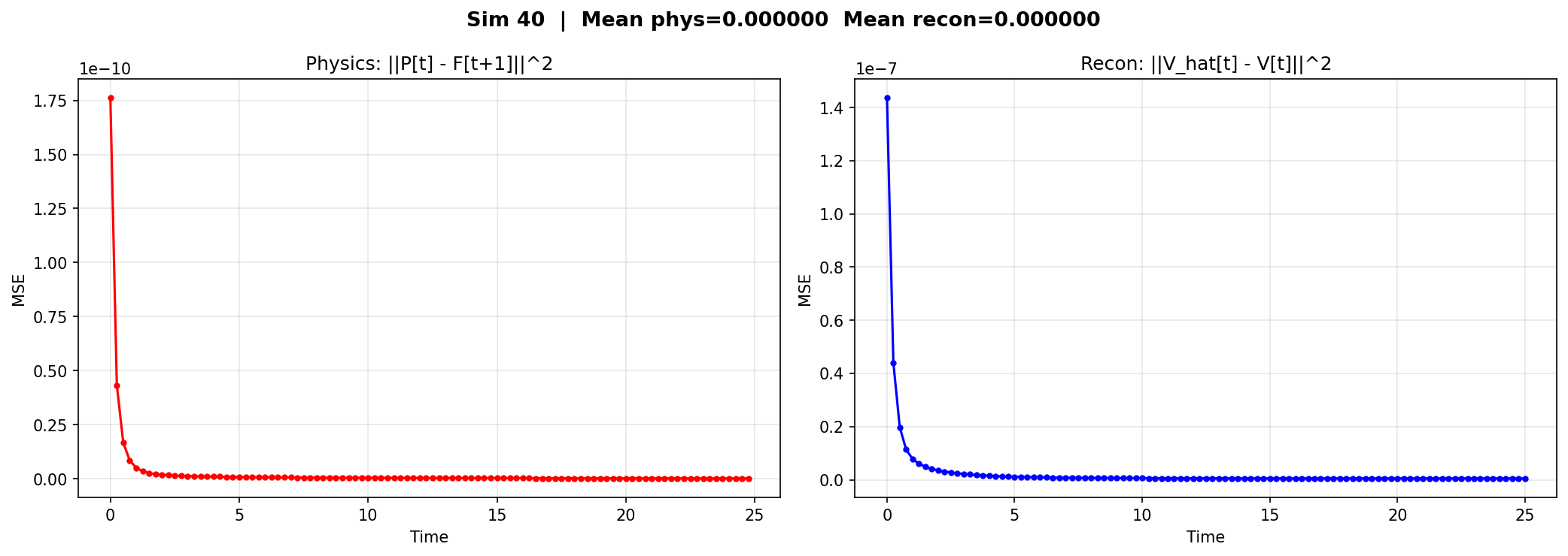
Table 4 and Fig. 3 summarize the quantitative results on 20 held-out simulations (10 diffusion, 10 mobility). Inference after training (Fig. 3(a)): the model is trained on 40 simulations and evaluated on the 20 held-out test simulations with 50 steps of test-time fine-tuning. It recovers $\alpha$ with overall mean absolute error (MAE $=$ $\frac{1}{n}\sum|\hat{\alpha}_{i}-\alpha_{i}|$) $=$ 0.0749 and $R^{2}_{\text{all}}=0.9245$, with excellent diffusion recovery ($R^{2}=0.9831$) but weaker mobility performance ($R^{2}=-0.33$), indicating that the trained model struggles to generalise for positive $\alpha$. Remarkably, zero-shot inference (Fig. 3(b)) achieves superior accuracy (MAE $=$ 0.0117, $R^{2}_{\text{all}}=0.9982$) with near-perfect recovery in both regimes, demonstrating that the SAFE loss alone provides sufficient supervision without any training data. Table 5 reports the field prediction quality: the mean SAFE loss (physics residual) is $9.6\times 10^{-8}$ and the mean reconstruction error is $4.3\times 10^{-8}$, confirming that the autoencoder faithfully reconstructs the input video while the SAFE operator accurately predicts the latent field evolution (Figs. 4–5).

Table 4: Transport coefficient recovery on 20 held-out simulations (10 diffusion, 10 mobility). SAFE-PIT-CM recovers $\alpha$ accurately for both negative (diffusion) and positive (mobility) values. The zero-shot mode, requiring no training data, achieves the best overall accuracy.

Setting	Sign	MAE	$\boldsymbol{R^{2}}$	$\boldsymbol{n}$ (sims)	True range
SAFE-PIT-CM (trained)	all	0.0749	0.9245	20	$[-0.7,0.7]$
	$\alpha<0$	–	0.9831	10	$[-0.7,-0.1]$
	$\alpha>0$	–	$-0.33$	10	$[0.1,0.7]$
SAFE-PIT-CM (zero-shot)	all	0.0117	0.9982	20	$[-0.7,0.7]$
	$\alpha<0$	–	1.0000	10	$[-0.7,-0.1]$
	$\alpha>0$	–	0.9674	10	$[0.1,0.7]$

Table 5: Field prediction quality (zero-shot, $N_{\text{sub}}=50$). The SAFE loss $\mathcal{L}_{\text{SAFE}}=\|P[t]-F[t\!+\!1]\|^{2}$ measures the physics residual; the reconstruction error $\mathcal{L}_{\text{recon}}=\|\hat{V}[t]-V[t]\|^{2}$ measures how faithfully the decoder reconstructs the input video. Both are mean squared errors averaged over all frames and simulations.

Regime	$n$	Mean $\mathcal{L}_{\text{SAFE}}$	Mean $\mathcal{L}_{\text{recon}}$
Diffusion ($\alpha<0$)	10	$1.4\times 10^{-9}$	$4.4\times 10^{-8}$
Mobility ($\alpha>0$)	10	$1.9\times 10^{-7}$	$2.8\times 10^{-8}$
All	20	$9.6\times 10^{-8}$	$4.3\times 10^{-8}$

(a) Inference after training (tested on held-out simulations).

(b) Zero-shot inference (no training data, fresh model per simulation).

Figure 3: Predicted vs. true transport coefficient $\alpha$ on 20 held-out simulations for both diffusion ($\alpha<0$, blue) and mobility ($\alpha>0$, red). (a) Inference after training: the model is trained on 40 simulations (sims 0–39) with $N_{\text{sub}}=50$, then evaluated on 20 held-out test simulations with 50 steps of test-time fine-tuning. MAE $=$ 0.0749, $R^{2}_{\text{all}}=0.9245$; diffusion $R^{2}=0.9831$, mobility $R^{2}=-0.33$. The trained model recovers diffusion accurately but fails on mobility. (b) Zero-shot inference: a fresh, randomly initialised model is optimised from scratch on each simulation individually (200 steps, no training data). MAE $=$ 0.0117, $R^{2}_{\text{all}}=0.9982$; diffusion $R^{2}=1.0000$, mobility $R^{2}=0.9674$.

Numerical stability is critical.

The sub-step ablation (Fig. 7 and Table 3) confirms that sufficient sub-stepping is essential for parameter recovery. For $N_{\text{sub}}\leq 2$, the von Neumann stability condition (Eq. 5) is violated for most of the data range, and mobility recovery collapses completely. At $N_{\text{sub}}=5$ the stability bound is satisfied for all $\alpha\in[0.1,0.7]$, and performance improves monotonically up to $N_{\text{sub}}=50$, which matches the original simulation save interval and reduces the per-step stability number by a factor of 50.

Zero-shot inference.

The zero-shot mode (Fig. 3(b)) demonstrates the power of the SAFE operator as an inductive bias. With no training data and no learned encoder (just a fresh random model), optimizing the SAFE loss on a single simulation for 200 steps recovers $\alpha$ with MAE $=$ 0.0117 and $R^{2}=0.9982$ across both diffusion and mobility regimes. This is possible because the Laplacian operator provides a direct, physics-grounded relationship between $\alpha$ and the frame-to-frame evolution: faster smoothing $\Rightarrow$ larger $|\alpha|$.

(a) $t=0$ (initial condition).

(b) $t=6.25$.

(c) $t=12.50$.

(d) $t=18.75$.

Figure 4: Diffusion ($\alpha<0$): example inference on simulation 40 ($\alpha_{\text{true}}=-0.198$, $\hat{\alpha}=-0.198$). Each row shows (left to right): input field $V[t]$, latent field $F[t]$, reconstructed field $\hat{V}[t]$, and absolute error $|P[t]-F[t+1]|$. The field evolves from a sharp Voronoi microstructure (a) through progressive smoothing (b, c) toward a diffused state (d).

(a) $t=0$ (initial condition).

(b) $t=6.25$.

(c) $t=12.50$.

(d) $t=18.75$.

Figure 5: Mobility ($\alpha>0$): example inference on simulation 90 ($\alpha_{\text{true}}=+0.198$, $\hat{\alpha}=+0.202$). Same layout as Fig. 4. The field sharpens over time: grain boundaries become increasingly pronounced as the reverse heat equation amplifies spatial gradients. Simulations 40 and 90 share the same $|\alpha|$ but opposite sign, illustrating the diffusion/mobility duality.

Figure 6: Per-frame error for the diffusion example (simulation 40). Left: SAFE loss $\|P[t]-F[t\!+\!1]\|^{2}$ (physics residual). Right: reconstruction error $\|\hat{V}[t]-V[t]\|^{2}$. Both errors are small and decrease over time as the field smooths. Mean physics error: ${\sim}10^{-7}$; mean reconstruction error: $5.5\times 10^{-6}$.

Training dynamics.

During Phase 1, $\alpha$ converges rapidly (within ${\sim}5$–10 epochs). The bounds penalty prevents early divergence but does not constrain the final values, which lie well within the allowed range. Phase 2 refines the reconstruction without disturbing the learned $\alpha$, thanks to the high SAFE loss weight.

3.3 Ablation studies

We conduct two ablation studies using zero-shot inference to isolate the effects of sub-stepping and temporal resolution on parameter recovery.

Effect of sub-step count $N_{\text{sub}}$.

Fig. 7 shows the $\alpha$ recovery MAE and $R^{2}$ as a function of $N_{\text{sub}}\in\{1,2,5,10,25,50\}$. For $N_{\text{sub}}\leq 2$, mobility ($\alpha>0$) suffers catastrophic failure due to the von Neumann stability violation (Eq. 5), while diffusion ($\alpha<0$) is unaffected by the stability constraint but still benefits from increased sub-stepping accuracy. At $N_{\text{sub}}=50$ (matching the simulation save interval), both regimes achieve near-perfect recovery.

Figure 7: Ablation: effect of sub-step count $N_{\text{sub}}$ on $\alpha$ recovery (zero-shot). Left: MAE (log scale). Right: $R^{2}$. For $N_{\text{sub}}\leq 2$, mobility ($\alpha>0$) collapses due to the stability violation; diffusion ($\alpha<0$) improves monotonically with $N_{\text{sub}}$.

Effect of temporal resolution.

Fig. 8 varies the frame step (using every $k$-th saved frame, $k\in\{1,2,5,10\}$). Reducing temporal resolution degrades mobility recovery while diffusion remains robust down to $T=21$ frames. At $T=11$ frames both regimes begin to degrade, suggesting a minimum temporal sampling requirement for accurate parameter identification.

Figure 8: Ablation: effect of temporal resolution (frame step) on $\alpha$ recovery (zero-shot). Left: MAE. Right: $R^{2}$. Mobility ($\alpha>0$) is more sensitive to reduced temporal resolution than diffusion ($\alpha<0$).

4 Discussion

SAFE-PIT-CM extends the differentiable-physics-as-a-layer paradigm from rigid-body dynamics [2] to continuum PDEs. The conceptual parallel is direct: both approaches embed a frozen physics solver inside a neural network and backpropagate through it. However, the numerical challenges differ. In rigid-body simulation, the solver is an LCP whose gradients can be computed analytically without stability concerns. In continuum PDE simulation, the explicit Euler integrator introduces a von Neumann stability constraint that, if ignored, silently corrupts the learned parameters. The SAFE operator—the frozen PDE layer at the heart of the autoencoder—resolves this issue and, to our knowledge, has not been addressed in prior work on differentiable PDE solvers.

Positive and negative transport coefficients.

We demonstrate recovery of both $\alpha=-D$ (diffusion, smoothing) and $\alpha=\kappa$ (mobility, sharpening). The mobility data is generated by time-reversing diffusion simulations, and the sign of $\alpha$ is provided as known process metadata. The SAFE operator and sign-aware estimation generalise naturally to more complex continuum models with multiple transport coefficients.

Numerical advantage of SAFE-PIT-CM for mobility.

Forward Euler integration of the mobility equation ($\alpha=\kappa>0$) is unconditionally unstable: the discrete amplification factor $G_{k}=1+\Delta t\cdot(-\alpha)\cdot\lambda_{k}$ exceeds unity for every non-constant Fourier mode, so high-frequency perturbations grow exponentially regardless of the time step. This is why mobility data must be generated via time reversal rather than direct simulation. SAFE-PIT-CM turns this limitation into an advantage: the attention-based estimator observes all frames simultaneously, including future states, so it can infer $|\alpha|$ from the rate of spatial sharpening without ever running the unstable forward problem. The SAFE operator always propagates in the numerically stable (diffusion) direction during training, even for mobility data, because the physics loss compares predicted and observed frames regardless of the sign of $\alpha$.

Explainability.

A key advantage of SAFE-PIT-CM over black-box video prediction models is interpretability. The latent-space transition is not a learned neural network but a frozen PDE operator with a single, physically meaningful parameter $\alpha$. Every prediction can be traced to (i) the encoder’s mapping from pixels to a physical field, (ii) a step-by-step Euler propagation with an inspectable $\hat{\alpha}$, and (iii) the decoder’s reconstruction. The predicted $\alpha$ is directly comparable to values measured by independent experiments (e.g., dilatometry, calorimetry), providing a built-in sanity check absent from black-box approaches. This positions SAFE-PIT-CM within the growing field of explainable scientific AI, where physical interpretability of learned models is as important as predictive accuracy.

Relation to PINNs.

PINNs [1] minimize the PDE residual at collocation points in the continuous domain. SAFE-PIT-CM minimizes the SAFE loss on the discrete grid, frame by frame, using the same finite-difference stencil as the data generator. This gives SAFE-PIT-CM two advantages: (i) the operator is exact (modulo floating-point precision) when the correct $\alpha$ is provided, eliminating approximation error; (ii) the method operates on video-like data without requiring pointwise field access.

Computational cost.

The dominant cost is the SAFE operator propagation: $\mathcal{O}(N_{\text{sub}}\times H\times W)$ per frame pair. For $N_{\text{sub}}=50$ and $128\times 128$ grids, each forward pass through the SAFE operator requires 50 convolutions. Training on 40 simulations with 101 frames each is fast on a single GPU. The attention-based estimator adds negligible overhead.

Limitations.

The current work uses synthetic data where the ground-truth PDE is known exactly. Applying SAFE-PIT-CM to experimental data introduces challenges: (i) measurement noise, (ii) non-periodic boundaries, (iii) unknown initial conditions, and (iv) possible model-form error if the true physics deviates from the assumed PDE. The explicit Euler sub-stepping is computationally expensive for stiff systems; implicit or spectral solvers could improve efficiency at the cost of more complex backward passes.

Future directions.

Extending to multi-parameter systems where positive and negative transport coefficients compete simultaneously is a natural follow-up. Applying the framework to experimental in-situ microscopy data, where a learned encoder maps raw pixel intensities to physical fields, is the ultimate goal.

5 Conclusion

We introduced SAFE-PIT-CM for recovering material parameters—both diffusion ($\alpha<0$) and mobility ($\alpha>0$)—from temporal sequences of field evolution. The key contributions are:

1. SAFE-PIT-CM: an autoencoder whose latent-space transition is a frozen PDE operator, enabling unsupervised material parameter recovery from video data.

2. The SAFE operator: a frozen finite-difference PDE operator with sub-stepping that is numerically stable and fully differentiable, enabling gradient-based parameter optimisation through the solver. We showed that without the SAFE operator, the learned transport coefficient collapses to an unphysical value dictated by numerical stability rather than the data—a failure mode not previously identified in the differentiable physics literature.

3. An attention-based parameter estimator that infers per-simulation material constants from the temporal structure of the field, without requiring ground-truth labels.

4. A zero-shot inference mode that recovers $\alpha$ from a single simulation with no training data, demonstrating that the SAFE-PIT-CM provides a sufficiently strong inductive bias for unsupervised parameter identification.

5. A two-phase training strategy that prevents encoder degeneracy and ensures robust convergence of material parameters.

The modular design of SAFE-PIT-CM supports extension to any PDE with a convolutional finite-difference discretisation—from diffusion and mobility to more complex multi-parameter continuum dynamics—opening a path toward automated material parameter identification from video observations of physical processes.

Code will be made available upon publication.

Appendix A Data generation

All training data is generated by numerically integrating the transport equation (Eq. 1) on a $128\times 128$ periodic grid with $\Delta x=\Delta y=0.5$, using forward Euler time integration with $\Delta t=0.005$ and 5000 steps per simulation. Snapshots are saved every 50 steps, yielding 101 frames per simulation (including the initial condition at $t=0$). The von Neumann stability condition (Eq. 4) is verified for each simulation before integration.

A.1 Initial conditions

The initial condition is a Voronoi tessellation of 15–35 grains/blobs on the periodic domain. Each grain centre is placed uniformly at random. For each grid point, the two nearest grain centres are identified, and the scalar field is set via a smooth $\tanh$ profile of the distance difference:

$$u_{i,j}=\tfrac{1}{2}\bigl(1+\tanh\bigl((d_{2}-d_{1}+\xi)\,/\,w\bigr)\bigr)$$ (13)

where $d_{1}$ and $d_{2}$ are the distances to the nearest and second-nearest grain centres, $w=2.5$ is the interface width, and $\xi$ is a spatially varying perturbation that introduces position-dependent boundary roughness. The composite field $u=\max_{i}(\eta_{i})$ takes values near 1 in grain interiors and ${\sim}0.5$ at grain boundaries, mimicking a polycrystalline microstructure.

A.2 Diffusion data ($\alpha=-D$): blobs

For diffusion (smoothing), 50 simulations are generated by integrating

$$\frac{\partial u}{\partial t}=-D\,\nabla^{2}u,\qquad\alpha=-D,\qquad|\alpha|\sim\mathcal{U}(0.1,\;0.7)$$ (14)

using forward Euler with $\Delta t=0.005$ for 5000 steps. The von Neumann stability condition requires

$$\Delta t\cdot|\alpha|\cdot\lambda_{\max}<2,\qquad\lambda_{\max}=\frac{8}{\Delta x\,\Delta y}=32$$ (15)

giving $|\alpha|<2/(0.005\times 32)=12.5$, which is satisfied for all sampled values. The simulation code verifies this condition before each run and reduces $\Delta t$ if needed.

Each simulation evolves from a sharp Voronoi microstructure toward a progressively smoother field as grain boundaries diffuse outward, producing soft, rounded structures we refer to as blobs. Snapshots are saved every $s=50$ steps, yielding 101 frames per simulation with $\Delta t_{\text{save}}=s\cdot\Delta t=0.25$.

A.3 Mobility data ($\alpha=\kappa$): grains

For mobility (sharpening), we exploit time-reversal symmetry. If $u(\mathbf{x},t)$ solves $\partial u/\partial t=-D\,\nabla^{2}u$ with $\alpha=-D<0$, then $v(\mathbf{x},t):=u(\mathbf{x},T-t)$ solves

$$\frac{\partial v}{\partial t}=\kappa\,\nabla^{2}v,\qquad\alpha=\kappa>0$$ (16)

We generate 50 additional simulations by time-reversing the diffusion data, i.e. flipping the saved frames along the time axis:

$$v[k]=u[T-k],\qquad k=0,\ldots,T$$ (17)

yielding 100 total simulations with transport coefficient $\alpha\in[-0.7,-0.1]\cup[0.1,0.7]$. The reversed sequences start from smooth blobs and evolve toward sharp grain boundaries, the hallmark of mobility (sharpening). Because the reversed data is never integrated directly, no stability condition needs to be satisfied for the positive transport coefficient.

A.4 Data splits

The first 80 simulations (80%) are used for training and the remaining 20 for validation and testing, giving a balanced mix of both signs. Each simulation is stored as a single array of shape $[T,N_{x},N_{y}]$ with associated metadata (transport coefficient, grid parameters, time step).

References

- [1] M. Raissi, P. Perdikaris, and G. E. Karniadakis. Physics-informed neural networks: A deep learning framework for solving forward and inverse problems involving nonlinear partial differential equations. Journal of Computational Physics, 378:686–707, 2019.
- [2] F. de Avila Belbute-Peres, K. Smith, K. Allen, J. Tenenbaum, and J. Z. Kolter. End-to-end differentiable physics for learning and control. In Advances in Neural Information Processing Systems, volume 31, 2018.
- [3] Z. Li, N. Kovachki, K. Azizzadenesheli, B. Liu, K. Bhatt, A. Stuart, and A. Anandkumar. Fourier neural operator for parametric partial differential equations. International Conference on Learning Representations, 2021.
- [4] A. Sanchez-Gonzalez, J. Godwin, T. Pfaff, R. Ying, J. Leskovec, and P. Battaglia. Learning to simulate complex physics with graph networks. Proceedings of the 37th International Conference on Machine Learning, 2020.
- [5] K. Um, R. Brand, Y. R. Fei, P. Holl, and N. Thuerey. Solver-in-the-loop: Learning from differentiable physics to interact with iterative PDE-solvers. Advances in Neural Information Processing Systems, 33, 2020.
- [6] G. E. Karniadakis, I. G. Kevrekidis, L. Lu, P. Perdikaris, S. Wang, and L. Yang. Physics-informed machine learning. Nature Reviews Physics, 3(6):422–440, 2021.
- [7] S. L. Brunton, B. R. Noack, and P. Koumoutsakos. Machine learning for fluid mechanics. Annual Review of Fluid Mechanics, 52:477–508, 2020.
- [8] A. Vaswani, N. Shazeer, N. Parmar, J. Uszkoreit, L. Jones, A. N. Gomez, Ł. Kaiser, and I. Polosukhin. Attention is all you need. In Advances in Neural Information Processing Systems, volume 30, 2017.